2014 06 26 - Townsend White Paper - Recent Declines in Ohio US LFP

1

Recent Declines in Ohio and United States Labor Force Participation: Implications for State of Ohio Revenues Neil Townsend John Glenn School of Public Affairs, The Ohio State University Jason Seligman, Editor June 2014

Executive Summary

Labor force participation (LFP), the percent of the population over age 16 that is employed or seeking

work, has fallen rapidly in the State of Ohio and the United States. From December 2007 to December

2013, U.S. LFP fell 3.2 percentage points and Ohio LFP dropped 3.5 percentage points. These declines

constitute the largest drop following any recession in the post‐Bretton Woods era.1 LFP matters to the

economy because it is an important determinant of labor supply. State budget analysts monitor LFP in

order to more accurately forecast future prospects for employment, labor income, and associated tax

revenues, among other reasons. This study investigates these recent declines in workforce participation,

examines female participation trends since 1973, and discusses implications for State of Ohio revenues.

Statistical analysis reveals that Ohio and U.S. LFP during recovery from the Great Recession is atypical of

historic recoveries since 1973. Specifically, year‐over‐year percentage changes in U.S. LFP are 0.9

percentage points lower during the current recovery. Consequently, previous recession recovery patterns

for LFP are less relevant. This paper considers particular factors which may account for differences in

order to allow better use of previous data for current and future forecasting purposes.

Of all factors analyzed, female labor force participation alone is found to robustly account for significant

changes between previous and current patterns. After de‐trending female LFP growth via synthetic

participation rates, multivariate analysis reveals that increased female entry in the labor force accounts

for 12.3 percent of year‐over‐year growth in U.S. LFP during previous recoveries. Because Ohio LFP trends

have been similar to the U.S. following recessions, it is reasonable to assume female LFP trends are

similar as well. As a result, it is recommended that state budget analysts account for this structural

change when forming revenue projections, reducing prospects for growth in recoveries accordingly.

1 The post‐Bretton Woods era of monetary management begins in March 1973 and is ongoing.

2

Acknowledgements:

Special thanks are due to Professor Seligman for his consistent advice and support. I would also like to

thank Fred Church, Isabel Louis, Astrid Arca, Kenneth Frey, Jeff Newman, and Professor Rob Greenbaum

for their general help and constructive feedback throughout the development process.

Lastly, I acknowledge the financial support of the Ohio Office of Budget and Management, the Ohio

Department of Taxation, and the John Glenn School of Public Affairs at The Ohio State University.

3

1.0 Introduction

Since the onset of the Great Recession2 in late 2007, labor force participation (LFP), the percent of the

population over age 16 that is employed or unemployed and seeking work,3 has fallen rapidly in the

State of Ohio and the United States as a whole. The U.S. labor force participation rate fell more than

three percentage points, to 62.8 percent, between December 2007 and December 2013; in Ohio, the

contemporaneous decline was 3.5 percentage points, to 63.3 percent. Labor force participation is

important for governments to gauge as it has implications for both revenues and expenditures, along

with more general implications for citizens welfare. This paper considers factors which may be

responsible for structural components of this decline – specifically, female labor force participation and

changes in capacity utilization. Of these, only female LFP is consistently found to be of importance,

however lagged capacity utilization does appear to hold some possible predictive power regarding LFP.

Prior to the Great Recession, female workforce participation increased from 1973 to 2000,

coinciding with overall growth in LFP, albeit at a faster rate. The ratio of female participation to overall

participation rates increased from 73% to nearly 90% and held steady during the 2000s (Figure 1).

2 According to the National Bureau of Economic Research (NBER), the Great Recession began in December 2007 and ended in June 2009. NBER defines a recession as “a period of falling economic activity spread across the economy, lasting more than a few months, normally visible in real GDP, real income, employment, industrial production, and wholesale‐retail sales” (nber.org). 3 More technically speaking, the Bureau of Labor Statistics defines the labor force participation rate as “the labor force as a percent of the civilian noninstitutional population” (bls.gov). I use the terms “labor force participation” and “labor force participation rate” interchangeably throughout this analysis.

70%

75%

80%

85%

90%

95%

1973 1978 1983 1988 1993 1998 2003 2008 2013

Figure 1: Ratio of Women Labor Force Participation Rate to Overall Labor Force Participation Rate 1973‐2013monthly, seasonally adjusted

Townsend, JGSPA; data source: BLS, June 2014

W LFP: LFP

4

What factors affect LFP? Is LFP during the current recovery meaningfully different from previous

recoveries since 1973? How much has increased female entry into the labor force contributed to overall

growth in LFP during the post‐Bretton Woods era? What are implications for the State of Ohio’s future

tax revenues?

Using bivariate and multivariate analysis, I investigate the recent declines in participation rates

in both Ohio and the United States, examine female participation trends since 1973, and discuss

implications for the State of Ohio’s tax revenues. Examining these labor trends should help the Ohio

Office of Budget and Management and the Ohio Department of Taxation in forming future revenue

projections and ultimately assist the State in effectively allocating its resources.

The second section of this paper provides background on Ohio and U.S. LFP trends in the post‐

Bretton Woods era and discusses recent studies on U.S. LFP decline since 2007. Section three describes

the data and methodology used to statistically compare recoveries and determine the extent to which

increased female workforce participation has contributed to overall growth in LFP. The fourth section

shares results of bivariate and multivariate analysis. Section five offers conclusions and discusses

implications for future State of Ohio revenues.

2.0 Background

This section provides background on labor force participation, beginning with overall trends,

distinguishing gender patterns, and offering a review of literature.

2.1 Labor force participation during the post‐Bretton Woods era4

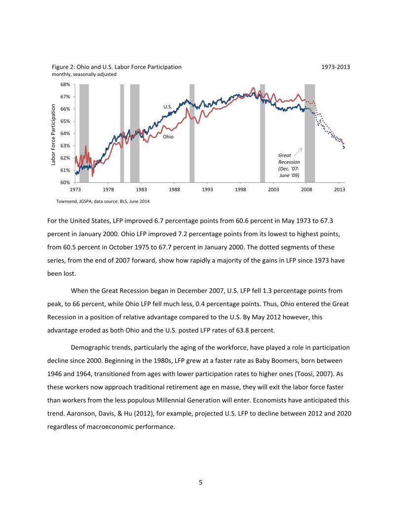
In both Ohio and the United States, labor force participation rates rose steadily from 1973 to 2000 as

seen in Figure 2.

4 I use March 1973 as the first month in this analysis because it marks the beginning of the post‐Bretton Woods system of monetary management. The International Monetary Fund notes that major currencies began floating against each other by this date (imf.org).

5

For the United States, LFP improved 6.7 percentage points from 60.6 percent in May 1973 to 67.3

percent in January 2000. Ohio LFP improved 7.2 percentage points from its lowest to highest points,

from 60.5 percent in October 1975 to 67.7 percent in January 2000. The dotted segments of these

series, from the end of 2007 forward, show how rapidly a majority of the gains in LFP since 1973 have

been lost.

When the Great Recession began in December 2007, U.S. LFP fell 1.3 percentage points from

peak, to 66 percent, while Ohio LFP fell much less, 0.4 percentage points. Thus, Ohio entered the Great

Recession in a position of relative advantage compared to the U.S. By May 2012 however, this

advantage eroded as both Ohio and the U.S. posted LFP rates of 63.8 percent.

Demographic trends, particularly the aging of the workforce, have played a role in participation

decline since 2000. Beginning in the 1980s, LFP grew at a faster rate as Baby Boomers, born between

1946 and 1964, transitioned from ages with lower participation rates to higher ones (Toosi, 2007). As

these workers now approach traditional retirement age en masse, they will exit the labor force faster

than workers from the less populous Millennial Generation will enter. Economists have anticipated this

trend. Aaronson, Davis, & Hu (2012), for example, projected U.S. LFP to decline between 2012 and 2020

regardless of macroeconomic performance.

60%

61%

62%

63%

64%

65%

66%

67%

68%

1973 1978 1983 1988 1993 1998 2003 2008 2013


Figure 2: Ohio and U.S. Labor Force Participation 1973‐2013monthly, seasonally adjusted

Ohio

U.S.

Great Recession(Dec. '07‐June '09)

Labor ForceParticipation

6

2.2 Labor force participation by gender

Analysis of monthly U.S. LFP by gender5 from 1973 to 2013 reveals different trajectories for men

and women as shown in Figure 3, below:

From March 1973 to April 2000, female LFP increased from 44.4 percent to its peak of 60.3 percent, a

nearly 16 percentage point increase; over this period women entered the labor force at elevated rates.6

Conversely, male LFP fell 10.4 percentage points from its high point of 79.5 percent in 1974 to 69.1

percent in December 2013. Thus, between 1973 and 2000, overall growth in LFP occurs as a result of

increases in LFP among women that overwhelmed decreases among men.

Despite different overall trajectories, workers of both genders have dropped out of the national

labor force since the Great Recession. Male LFP declined four percentage points from December 2007 to

December 2013, while female LFP fell a lesser 2.5 percentage points over the same duration. The

average ages among female and male participants are listed along the bottom of Figure 3, above the

time‐axis. They reveal a convergence in average ages across genders over this period.7,8

Turning next to Ohio, the story is similar. However, Ohio participation numbers by gender are

only available from 1981 on and then only annually. To summarize those data, Figure 4 illustrates Ohio

participation trends for both genders:

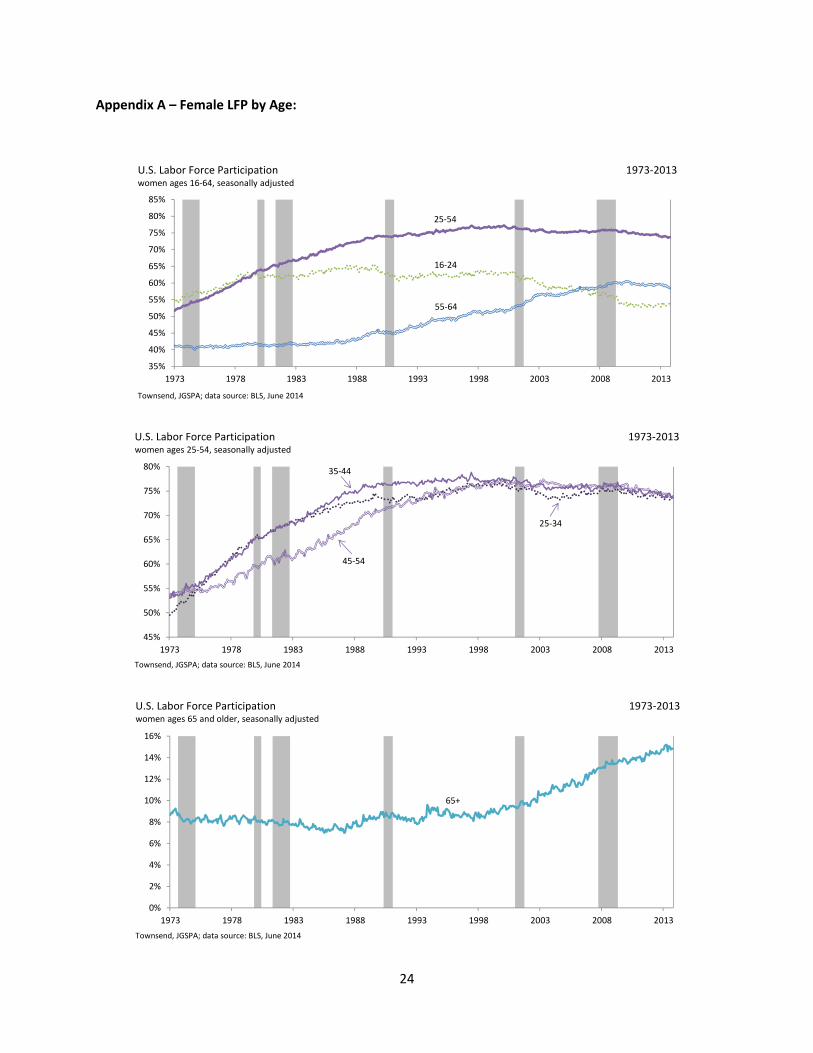
5 Ohio LFP data by gender is not available at this frequency. 6 Goldin (2006) dubs increased female workforce entry over this period as the “Quiet Revolution” and attributes much of this growth to higher prevalence of contraception use and divorce. 7 See Appendix A for a breakdown of female LFP by age. 8 See Appendix B for full explanation of calculations for average age of U.S. labor force by gender.

57%

62%

67%

72%

77%

82%

37%

42%

47%

52%

57%

62%

1973 1978 1983 1988 1993 1998 2003 2008 2013

Figure 3: U.S. Labor Force Participation by Gender 1973‐2013

monthly, seasonally adjusted

Townsend, JGSPA; data source: BLS, June 20141Author's calculations. See Appendix A for methodology.

shaded area highlights Dec. 2007 ‐Dec. 2013

men

women

36.237.5

36.337.3

37.838.1

40.039.9

41.741.7

36.937.6

38.739.0

41.040.9

women LFP

men LFP

womenmen

average age of labor force by gender1

7

From 1981 to 2013, Ohio women exhibit the same upward trend as U.S. women while LFP for both Ohio

and U.S. men trend downward. Ohio women, however, have lost their relative advantage in

participation rates since 2008. That year, LFP for Ohio women was nearly three percentage points higher

than that of U.S. women, 62.4 versus 59.5 percent. By 2012, however, this difference no longer existed.

Though participation levels for both Ohio and U.S. men have also declined since 2008, a distinction

exists in that, relative to the United States, Ohio men participate at a somewhat lesser rate ‐‐trailing by

1.7 percentage points, 68 percent to 69.7 percent.

2.3 Labor force participation studies

Previous research into labor force participation almost exclusively focuses on developments at the

national level. Since the Great Recession, most of the literature focuses on quantitatively determining

how much the recent decline in U.S. LFP reflects structural factors like long‐run demographic trends

versus cyclical factors like recessions and recoveries.9 Both cyclical and structural factors affect LFP;

where scholars disagree is the extent to which these types of changes factor into the drop.10 Though I do

not wade into the structural versus cyclical debate, in this white paper I do attempt to examine the

9 Cyclical changes are more temporary or short‐lived while structural changes are more permanent or long‐lived (Swanson, 2012). 10 Generally speaking, if LFP decline is more cyclical in nature then one would expect LFP to rise as the economy grows. More structural changes suggest less improvement over time.

65%

70%

75%

80%

85%

45%

50%

55%

60%

65%

1981 1989 1997 2005 2013

Figure 4: Ohio and U.S. Labor Force Participation by Gender 1981‐2013

annually, seasonally adjusted


women: Ohio, US

men: Ohio, US

women LFP m

en LFP

8

extent to which increased female entry from 1973 to 2000—a period of structural change for the

economy—has contributed to overall LFP growth.11

A variety of trends, events, and policies affect participation levels and it is often difficult to

isolate the exact impact of each factor. Aside from the business cycle and the aging of the workforce

(Maki, Davig, & Newland, 2012), other possible factors considered in the literature include the decline in

manufacturing employment (Charles, Hurst, & Notowidigdo, 2013), lower workforce entry rates (Nichols

& Lindner, 2013), increases in disability claims (Ruffing, 2013; Fujita, 2013), and extensions of

unemployment insurance (Van Zandweghe, 2012; Nichols & Lindner, 2013). In upcoming years, the

Congressional Budget Office predicts that effects of the Affordable Care Act will reduce worker

incentives to participate in the labor force and have a negative impact on participation rates (2014).

Several analyses employ noteworthy methodology. Hotchkiss & Rios‐Avila (2013) construct a

counterfactual distribution by re‐weighting post‐recession observations so that they resemble pre‐

recession counterparts in order to make direct comparisons across samples that are usually not possible

given the nature of economic data. In this line, I construct counterfactual LFP evolutions over the 1973‐

2000 period via synthetic data (more detail is found below, as part of the discussion of methods). Van

Zandweghe (2012) performs separate Beveridge‐Nelson decompositions for men and women to see if

structural or cyclical factors vary by gender. To wit, I also examine participation trends by gender.

While the literature specifically on labor force participation and state tax revenues is sparse,

Felix & Watkins (2013) predict that the graying of the population implies both income and sales tax

revenue per capita will decrease in every state as older people tend to both earn and consume less.

Because projected population growth in Ohio through 2030 is minimal, the state may experience more

decreases in revenues than others. How much Baby Boomers will reduce their consumption is unclear

though, especially if they stay in the labor force at higher rates relative to the norm.

Specific literature on Ohio’s labor force participation since 2007 is lacking though some research

touches on Ohio’s employment picture. Using BLS data through 2012, Hall & Greene (2013) analyze the

state’s employment by industry since 2007. Aside from improvements in mining & logging and

education and health services, they report that recoveries in most sectors since 2007 are incomplete

and lag the national average. These findings are consistent with Seligman & Vitale (2013), who also note

11 Stockell (2011) analyzes structural and cyclical budget deficits in light of the Great Recession and discusses implications for Ohio withholdings.

9

improvement in manufacturing, professional and business services, and leisure and hospitality from the

beginning of the current recovery through the first quarter of 2013.

3.0 Methodology & Data

This section begins with a discussion of methods. Following the discussion of methods I describe the

data employed in analysis.

3.1 Methodology for bivariate analysis

In order to statistically compare labor force participation during the 2009 recovery to typical recoveries,

it is necessary to see how LFP usually fares following economic recessions, To address this I focus on

experiences over the post‐Bretton Woods era. In all, six recessions occurred between March 1973 and

December 2013.12

Using monthly participation data, it is possible to observe how Ohio and U.S. LFP historically

perform at various months into economic recovery and compare LFP figures during the current recovery

to these averages using a t‐test to determine if they are meaningfully different.13 For example, LFP

during July 2009, the first month of the 2009 recovery, is statistically compared to average LFP for five

previous recoveries. The t‐statistic is then used to calculate the p‐value using a standard one‐tailed test.

These comparisons are also done for month‐over‐month and year‐over‐year percentage changes.

Statistically significant differences suggest that the 2009 recovery is atypical of historical recoveries.

To the extent that differences between this and previous recoveries are attributable to a one‐

time cultural phenomenon of female labor force entry, expecting reversion to previous trends is ill‐

advised. In this case, examining LFP during previous recoveries may no longer be as useful a guide to

predicting labor force trends or behaviors during current and future recoveries; instead, it would be

advisable for state budget analysts to account for the structural shift in female labor force engagement.

12 The recession periods are: (1) November 1973‐March 1975 (16 months); (2) January 1980‐July 1980 (6 months); (3) July 1981‐November 1982 (16 months); (4) July 1990‐March 1991 (8 months); (5) March 2001‐November 2001 (8 months); (6) December 2007‐June 2009 (18 months). 13 See Appendix C for a description of the t‐test.

10

One way to test for this is to de‐trend the growth in U.S. female participation and build a

synthetic recovery data set with which to perform the same statistical tests used to compare Ohio and

U.S. LFP. This strategy is engaged via the construction of synthetic LFP rates in order to compare LFP

rates during the 2009 recovery to average LFP rates during a synthetic recovery that assumes no growth

in female LFP. If comparisons of t‐test results reveal that U.S. p‐values are less or no longer statistically

significant, it would suggest a structural component to the decline in U.S. LFP that has not garnered

much attention. Though Ohio data by age and gender are not available at monthly frequency, it is

possible to generalize U.S. results to Ohio because Ohio patterns for LFP have been similar to the U.S.

following recessions.

Before de‐trending growth in female participation, it is important to seasonally adjust labor

force levels for all age cohorts.14 Because LFP is the quotient of the labor force and non‐institutional

population, it is necessary to de‐trend growth in both labor force and population levels for female age

cohorts: {16‐24, 25‐34, 35‐44, 45‐54, 55‐64, 65+} and then construct synthetic labor force and

population levels for each subset.

The first step in creating synthetic labor force levels is to calculate the compound growth rate

from March 1973 to December 2013. The formula to compute the compound growth rate is,

(1) ⁄

1

Where: = rate; Y = end value; X = initial value; T = number of periods.15 The second step is to calculate

the monthly percent change in the labor force using the equation,

(2) ∆% 100

Where: t = current value; (t‐1) = old value. For example, the monthly percent change in 65 and older

female labor force levels from March 1973 (1,028) to April 1973 (1,058) is 2.88 percent.

14 BLS does not seasonally adjust labor force levels for ages 16‐24, 55‐64, and 65+ by gender. These data are seasonally adjusted using the TRAMO/SEATS parametric (model‐based) method (see Monsell, 2009 for more detail). BLS does not seasonally adjust population levels when computing the labor force participation rates. 15 To illustrate, the compound growth rate for the 65 and older female labor force (in thousands) is computed:

0.263,6451,028

/

1

Where: 0.26 = rate; 3,645 = December 2013 total labor force; 1,028 = March 1973 total labor force; 489 = number of months between March 1973 and December 2013.

11

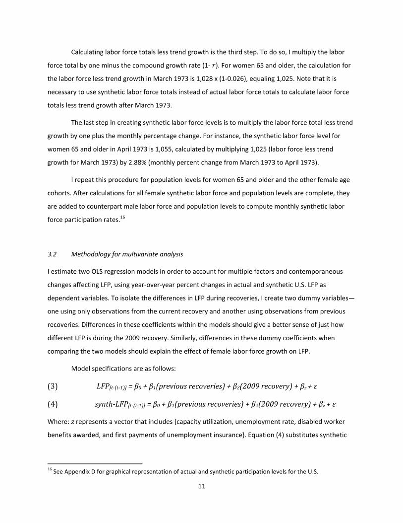
Calculating labor force totals less trend growth is the third step. To do so, I multiply the labor

force total by one minus the compound growth rate (1‐ ). For women 65 and older, the calculation for

the labor force less trend growth in March 1973 is 1,028 x (1‐0.026), equaling 1,025. Note that it is

necessary to use synthetic labor force totals instead of actual labor force totals to calculate labor force

totals less trend growth after March 1973.

The last step in creating synthetic labor force levels is to multiply the labor force total less trend

growth by one plus the monthly percentage change. For instance, the synthetic labor force level for

women 65 and older in April 1973 is 1,055, calculated by multiplying 1,025 (labor force less trend

growth for March 1973) by 2.88% (monthly percent change from March 1973 to April 1973).

I repeat this procedure for population levels for women 65 and older and the other female age

cohorts. After calculations for all female synthetic labor force and population levels are complete, they

are added to counterpart male labor force and population levels to compute monthly synthetic labor

force participation rates.16

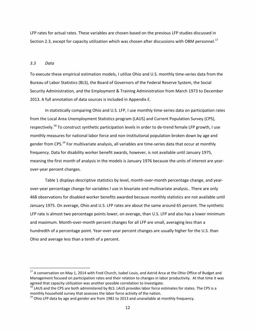
3.2 Methodology for multivariate analysis

I estimate two OLS regression models in order to account for multiple factors and contemporaneous

changes affecting LFP, using year‐over‐year percent changes in actual and synthetic U.S. LFP as

dependent variables. To isolate the differences in LFP during recoveries, I create two dummy variables—

one using only observations from the current recovery and another using observations from previous

recoveries. Differences in these coefficients within the models should give a better sense of just how

different LFP is during the 2009 recovery. Similarly, differences in these dummy coefficients when

comparing the two models should explain the effect of female labor force growth on LFP.

Model specifications are as follows:

(3) LFP[t‐(t‐1)]=β0+β1(previousrecoveries)+β2(2009recovery)+βz+ε

(4) synth‐LFP[t‐(t‐1)]=β0+β1(previousrecoveries)+β2(2009recovery)+βz+ε

Where: zrepresents a vector that includes {capacity utilization, unemployment rate, disabled worker

benefits awarded, and first payments of unemployment insurance}. Equation (4) substitutes synthetic

16 See Appendix D for graphical representation of actual and synthetic participation levels for the U.S.

12

LFP rates for actual rates. These variables are chosen based on the previous LFP studies discussed in

Section 2.3, except for capacity utilization which was chosen after discussions with OBM personnel.17

3.3 Data

To execute these empirical estimation models, I utilize Ohio and U.S. monthly time‐series data from the

Bureau of Labor Statistics (BLS), the Board of Governors of the Federal Reserve System, the Social

Security Administration, and the Employment & Training Administration from March 1973 to December

2013. A full annotation of data sources is included in Appendix E.

In statistically comparing Ohio and U.S. LFP, I use monthly time‐series data on participation rates

from the Local Area Unemployment Statistics program (LAUS) and Current Population Survey (CPS),

respectively.18 To construct synthetic participation levels in order to de‐trend female LFP growth, I use

monthly measures for national labor force and non‐institutional population broken down by age and

gender from CPS.19 For multivariate analysis, all variables are time‐series data that occur at monthly

frequency. Data for disability worker benefit awards, however, is not available until January 1975,

meaning the first month of analysis in the models is January 1976 because the units of interest are year‐

over‐year percent changes.

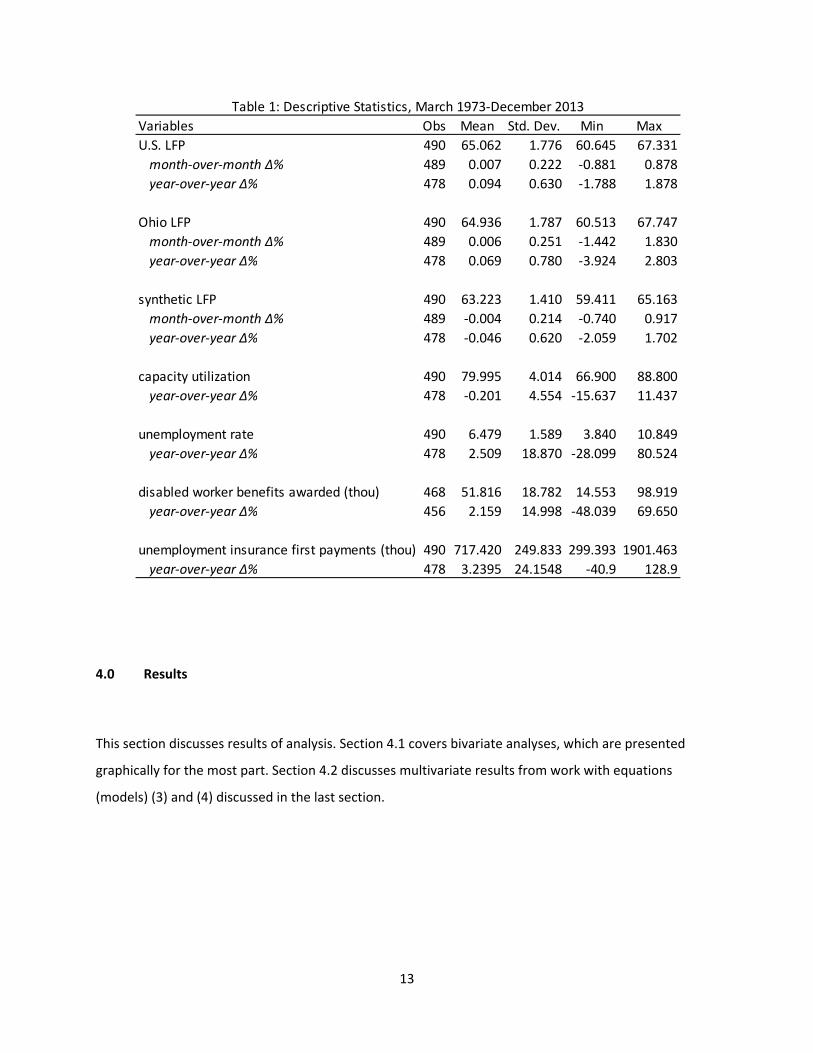
Table 1 displays descriptive statistics by level, month‐over‐month percentage change, and year‐

over‐year percentage change for variables I use in bivariate and multivariate analysis.. There are only

468 observations for disabled worker benefits awarded because monthly statistics are not available until

January 1975. On average, Ohio and U.S. LFP rates are about the same around 65 percent. The synthetic

LFP rate is almost two percentage points lower, on average, than U.S. LFP and also has a lower minimum

and maximum. Month‐over‐month percent changes for all LFP are small, averaging less than a

hundredth of a percentage point. Year‐over‐year percent changes are usually higher for the U.S. than

Ohio and average less than a tenth of a percent.

17 A conversation on May 1, 2014 with Fred Church, Isabel Louis, and Astrid Arca at the Ohio Office of Budget and Management focused on participation rates and their relation to changes in labor productivity. At that time it was agreed that capacity utilization was another possible correlation to investigate. 18 LAUS and the CPS are both administered by BLS. LAUS provides labor force estimates for states. The CPS is a monthly household survey that assesses the labor force activity of the nation. 19 Ohio LFP data by age and gender are from 1981 to 2013 and unavailable at monthly frequency.

13

4.0 Results

This section discusses results of analysis. Section 4.1 covers bivariate analyses, which are presented

graphically for the most part. Section 4.2 discusses multivariate results from work with equations

(models) (3) and (4) discussed in the last section.

Variables Obs Mean Std. Dev. Min Max

U.S. LFP 490 65.062 1.776 60.645 67.331

month‐over‐month Δ% 489 0.007 0.222 ‐0.881 0.878

year‐over‐year Δ% 478 0.094 0.630 ‐1.788 1.878

Ohio LFP 490 64.936 1.787 60.513 67.747

month‐over‐month Δ% 489 0.006 0.251 ‐1.442 1.830

year‐over‐year Δ% 478 0.069 0.780 ‐3.924 2.803

synthetic LFP 490 63.223 1.410 59.411 65.163

month‐over‐month Δ% 489 ‐0.004 0.214 ‐0.740 0.917

year‐over‐year Δ% 478 ‐0.046 0.620 ‐2.059 1.702

capacity utilization 490 79.995 4.014 66.900 88.800

year‐over‐year Δ% 478 ‐0.201 4.554 ‐15.637 11.437

unemployment rate 490 6.479 1.589 3.840 10.849

year‐over‐year Δ% 478 2.509 18.870 ‐28.099 80.524

disabled worker benefits awarded (thou) 468 51.816 18.782 14.553 98.919

year‐over‐year Δ% 456 2.159 14.998 ‐48.039 69.650

unemployment insurance first payments (thou) 490 717.420 249.833 299.393 1901.463

year‐over‐year Δ% 478 3.2395 24.1548 ‐40.9 128.9

Table 1: Descriptive Statistics, March 1973‐December 2013

14

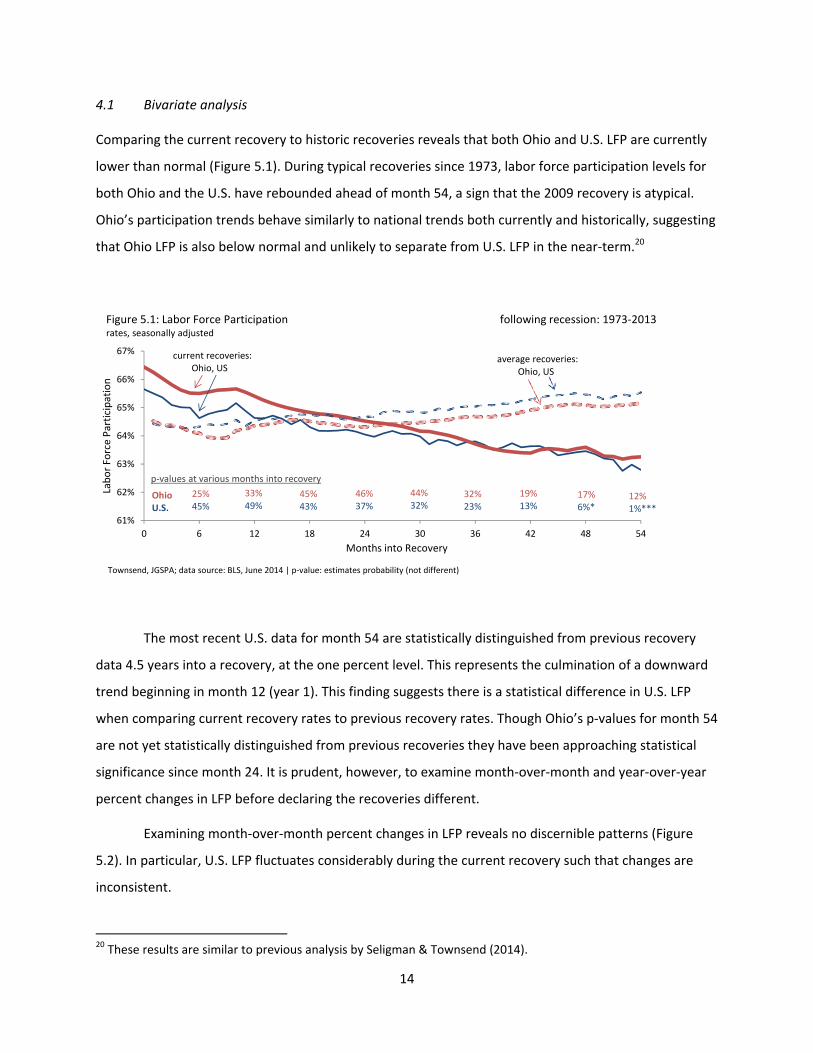
4.1 Bivariate analysis

Comparing the current recovery to historic recoveries reveals that both Ohio and U.S. LFP are currently

lower than normal (Figure 5.1). During typical recoveries since 1973, labor force participation levels for

both Ohio and the U.S. have rebounded ahead of month 54, a sign that the 2009 recovery is atypical.

Ohio’s participation trends behave similarly to national trends both currently and historically, suggesting

that Ohio LFP is also below normal and unlikely to separate from U.S. LFP in the near‐term.20

The most recent U.S. data for month 54 are statistically distinguished from previous recovery

data 4.5 years into a recovery, at the one percent level. This represents the culmination of a downward

trend beginning in month 12 (year 1). This finding suggests there is a statistical difference in U.S. LFP

when comparing current recovery rates to previous recovery rates. Though Ohio’s p‐values for month 54

are not yet statistically distinguished from previous recoveries they have been approaching statistical

significance since month 24. It is prudent, however, to examine month‐over‐month and year‐over‐year

percent changes in LFP before declaring the recoveries different.

Examining month‐over‐month percent changes in LFP reveals no discernible patterns (Figure

5.2). In particular, U.S. LFP fluctuates considerably during the current recovery such that changes are

inconsistent.

20 These results are similar to previous analysis by Seligman & Townsend (2014).

61%

62%

63%

64%

65%

66%

67%

0 6 12 18 24 30 36 42 48 54

Figure 5.1: Labor Force Participation following recession: 1973‐2013rates, seasonally adjusted

Months into Recovery

average recoveries: Ohio, US

Townsend, JGSPA; data source: BLS, June 2014 | p‐value: estimates probability (not different)

current recoveries: Ohio, US

OhioU.S.

25%45%

33%49%

45%43%

46%37%

44%32%

32%23%

19%13%

17%6%*

12%1%***

p‐values at various months into recovery

Labor Force Participation

15

Having noted inconsistency in the figure above, differences are statistically significant at the five percent

level or better in the first and last year of the current recovery as well as at the two‐year mark, but

insignificant at other months. The median p‐value (3%), however, is significant at the five percent level.

Ohio p‐values are only significant at the one percent level at month 36, though p‐values for months 12,

30, and 48 are statistically significant at the ten percent level. Because there is so much variation in

these p‐values, it is also worthwhile to examine year‐over‐year changes in LFP. Analyzing year‐over‐year

changes best highlights the unusual path of LFP throughout the 2009 recovery (Figure 5.3).

‐1.0%

‐0.8%

‐0.6%

‐0.4%

‐0.2%

0.0%

0.2%

0.4%

0.6%

0 6 12 18 24 30 36 42 48 54

Figure 5.2: Labor Force Participation following recession: 1973‐2013month‐over‐month percent change, seasonally adjusted






OhioU.S.

42%1%***

Month‐over‐month

Δ% LFP

7%*3%**

40%16%

12%0%***

7%*46%

0%***36%

17%32%

7%*0%***

42%0%***

‐3.0%

‐2.5%

‐2.0%

‐1.5%

‐1.0%

‐0.5%

0.0%

0.5%

1.0%

1.5%

0 6 12 18 24 30 36 42 48 54

Figure 5.3: Labor Force Participation following recession: 1973‐2013year‐over‐year percent change, seasonally adjusted





Year‐over‐year

Δ% LFP


OhioU.S.

‐‐‐‐‐‐

15%0%***

4%**12%

0%***6%*

1%***22%

0%***6%*

0%***1%***

18%3%**

8%*0%***

16

Using year‐over‐year data, one can more easily see that LFP is much lower than in typical recoveries. In

fact I observe no positive year‐over‐year growth in any month of the current recovery. This finding is

consistent with the continuous downward trend in LFP levels depicted in Figure 5.1.

Historically, the U.S. has been a more consistent generator of positive LFP than Ohio during

economic recoveries. Though Ohio has fared worse than the U.S. in the current recovery, with LFP falling

by one or more percent each month between months 18 to 43, Ohio has fared better than the US in the

fifth year of recovery. Whether this break in trend can and will persist going forward is unclear.

Taking medians of the series of individual p‐values for both Ohio and the U.S. listed at the

bottom of Figure 5.3 (3 percent and 4 percent, respectively) allows one to statistically distinguish this

recovery from previous recoveries at the five percent level. Furthermore, while individual Ohio p‐values

past month 48 suggest more similarity with previous recoveries it is still the case that changes in LFP are

persistently negative.

Focusing next on women, de‐trending growth in female LFP reveals that participation rates are

lower during a synthetic recovery than during the average recovery (Figure 6.1):

60%

61%

62%

63%

64%

65%

66%

67%

0 6 12 18 24 30 36 42 48 54

Figure 6.1: U.S. Labor Force Participation following recession: 1973‐2013rates, seasonally adjusted, with a synthetic recovery


Townsend, JGSPA; data sources: BLS, June 2014 | p‐value: estimates probability (not different)1Synthetic recovery detrends growth in female LFP over 1973‐2013.

synthetic recovery1

average recoverycurrent recovery


45%14%

49%15%

43%23%

37%22%

32%25%

23%35%

13%47%

6%*30%

1%***7%*

averagesynthetic


17

The slope is slightly flatter for the synthetic recovery. Consistent with this finding, statistical analysis

reveals that the recent p‐values are less different. An interpretation of that observation is that once one

accounts for the structural entry of females into the labor force between 1973 and 2000 the current

recovery does not look as different—in terms of levels of LFP.

In comparing LFP by rates (Figure 5.1), U.S. data for month 54 proved significant at the one

percent level, indicating a meaningful difference. After de‐trending growth in female LFP, however, U.S.

data for month 54 are now only statistically significant at then ten percent level and month 48 is no

longer statistically significant at all. However, the median p‐value is lower for the synthetic recovery (24

percent) than the average recovery (37 percent). These mixed results invite further analysis by month‐

over‐month and year‐over‐year percent changes.

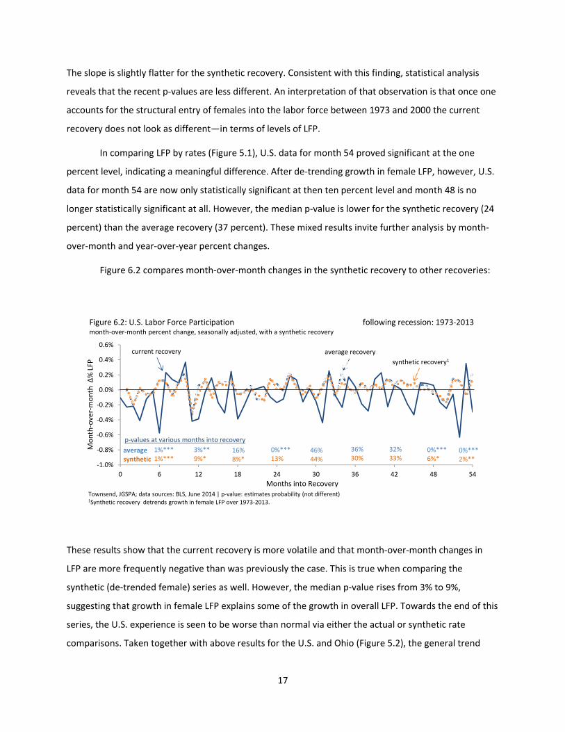
Figure 6.2 compares month‐over‐month changes in the synthetic recovery to other recoveries:

These results show that the current recovery is more volatile and that month‐over‐month changes in

LFP are more frequently negative than was previously the case. This is true when comparing the

synthetic (de‐trended female) series as well. However, the median p‐value rises from 3% to 9%,

suggesting that growth in female LFP explains some of the growth in overall LFP. Towards the end of this

series, the U.S. experience is seen to be worse than normal via either the actual or synthetic rate

comparisons. Taken together with above results for the U.S. and Ohio (Figure 5.2), the general trend

‐1.0%

‐0.8%

‐0.6%

‐0.4%

‐0.2%

0.0%

0.2%

0.4%

0.6%

0 6 12 18 24 30 36 42 48 54

Figure 6.2: U.S. Labor Force Participation following recession: 1973‐2013month‐over‐month percent change, seasonally adjusted, with a synthetic recovery


synthetic recovery1average recoverycurrent recovery


Month‐over‐month

Δ% LFP


averagesynthetic

1%***1%***

3%**9%*

16%8%*

0%***13%

46%44%

36%30%

32%33%

0%***6%*

0%***2%**

18

that emerges in the fifth year of recovery is that Ohio’s underperformance is masked by even worse

performance nationally.

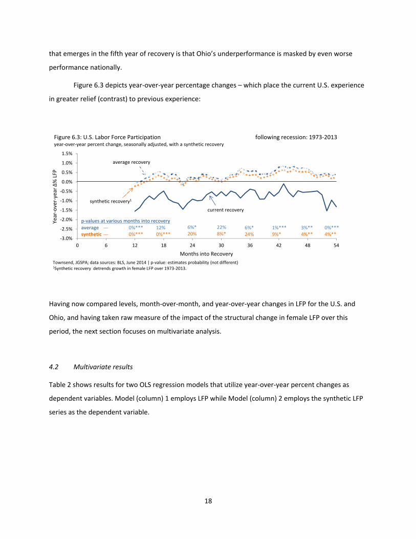
Figure 6.3 depicts year‐over‐year percentage changes – which place the current U.S. experience

in greater relief (contrast) to previous experience:

Having now compared levels, month‐over‐month, and year‐over‐year changes in LFP for the U.S. and

Ohio, and having taken raw measure of the impact of the structural change in female LFP over this

period, the next section focuses on multivariate analysis.

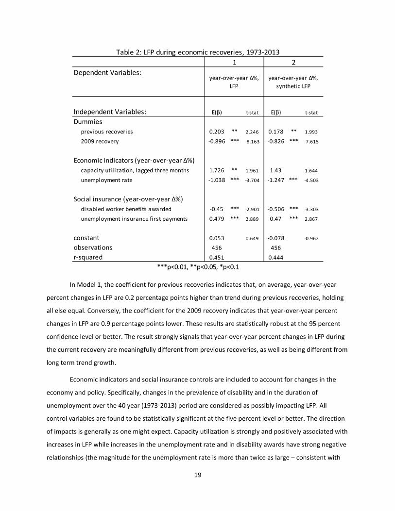
4.2 Multivariate results

Table 2 shows results for two OLS regression models that utilize year‐over‐year percent changes as

dependent variables. Model (column) 1 employs LFP while Model (column) 2 employs the synthetic LFP

series as the dependent variable.

‐3.0%

‐2.5%

‐2.0%

‐1.5%

‐1.0%

‐0.5%

0.0%

0.5%

1.0%

1.5%

0 6 12 18 24 30 36 42 48 54

Figure 6.3: U.S. Labor Force Participation following recession: 1973‐2013year‐over‐year percent change, seasonally adjusted, with a synthetic recovery


synthetic recovery1

average recovery

current recovery

Year‐over‐year Δ% LFP



averagesynthetic

‐‐‐‐‐‐

0%***0%***

12%0%***

6%*20%

22%8%*

6%*24%

1%***9%*

3%**4%**

0%***4%**

19

In Model 1, the coefficient for previous recoveries indicates that, on average, year‐over‐year

percent changes in LFP are 0.2 percentage points higher than trend during previous recoveries, holding

all else equal. Conversely, the coefficient for the 2009 recovery indicates that year‐over‐year percent

changes in LFP are 0.9 percentage points lower. These results are statistically robust at the 95 percent

confidence level or better. The result strongly signals that year‐over‐year percent changes in LFP during

the current recovery are meaningfully different from previous recoveries, as well as being different from

long term trend growth.

Economic indicators and social insurance controls are included to account for changes in the

economy and policy. Specifically, changes in the prevalence of disability and in the duration of

unemployment over the 40 year (1973‐2013) period are considered as possibly impacting LFP. All

control variables are found to be statistically significant at the five percent level or better. The direction

of impacts is generally as one might expect. Capacity utilization is strongly and positively associated with

increases in LFP while increases in the unemployment rate and in disability awards have strong negative

relationships (the magnitude for the unemployment rate is more than twice as large – consistent with

Dependent Variables:

Independent Variables: E(β) t‐stat E(β) t‐stat

Dummies

previous recoveries 0.203 ** 2.246 0.178 ** 1.993

2009 recovery ‐0.896 *** ‐8.163 ‐0.826 *** ‐7.615

Economic indicators (year‐over‐year Δ%)

capacity util ization, lagged three months 1.726 ** 1.961 1.43 1.644

unemployment rate ‐1.038 *** ‐3.704 ‐1.247 *** ‐4.503

Social insurance (year‐over‐year Δ%)

disabled worker benefits awarded ‐0.45 *** ‐2.901 ‐0.506 *** ‐3.303

unemployment insurance first payments 0.479 *** 2.889 0.47 *** 2.867

constant 0.053 0.649 ‐0.078 ‐0.962

observations 456 456

r‐squared 0.451 0.444

***p<0.01, **p<0.05, *p<0.1

Table 2: LFP during economic recoveries, 1973‐2013

1 2

year‐over‐year Δ%,

LFP

year‐over‐year Δ%,

synthetic LFP

20

the notion that disability is eligibility‐constrained to a greater degree.) The relationship between first

payments for unemployment is further included to measure a differential between changes in

unemployment uptake and in unemployment persistence. While the interpretation of this coefficient is

not as obvious, it generally suggests that increases in unemployment rolls alone are not correlated with

reductions in LFP. The positive coefficient may be an artifact of population growth from 1973 to 2013. In

any case, the inclusion of this variable generally absorbs trends that might otherwise confound

measures across the rest of the multivariate specification.

In sensitivity analysis exercises, after noting that the capacity utilization variable carried the

weakest t‐statistic, this variable was targeted for further investigation. To this end the capacity

utilization variable was lagged in varying degree in order to consider the impact of other lags for the

findings reported here. Lagging capacity utilization more or less than three months does not improve

model fit or meaningfully alter conclusions. The three month lag duration appears to best capture a

relationship between capacity utilization and LFP over this period of modern history.

Model 2 uses the year‐over‐year percent change in synthetic LFP as the dependent variable. In

line with expectations, the coefficient for previous recoveries declines (being 0.025 percentage points

lower) relative to Model 1. Accordingly, the percent difference in the coefficients indicates that growth

in female participation accounts for 12.3 percent of the year‐over‐year percent increase in LFP during

previous recoveries. The coefficient for the 2009 recovery is 0.07 percentage points lower than the

coefficient in the previous model, consistent with the notion that de‐trending female LFP growth

attenuates the variation in LFP. Furthermore, the t‐statistics for the dummy variables are somewhat

weaker, as is the explanatory power of the model. Coefficients for the unemployment rate, disabled

worker benefits, and unemployment insurance first payments are still statistically significant at the one

percent level.

Perhaps most notably across controls, the coefficient for capacity utilization is no longer

significant—being just outside of even the weak (90 percent) confidence interval. The best that can be

said based on this analysis is that lagged capacity utilization appears to hold some possible predictive

power for LFP. While such a finding is consistent with a theory that increased demand for labor draws

supplies off the ‘sidelines,’ this result appears sensitive to specifications. It is possible that the

relationship is non‐linear in some important way – when capacity utilization is very high or very low, for

example. Saying more than this is not possible given the (necessarily) limited focus of this white paper.

21

5.0 Conclusion

This study investigates recent declines in labor force participation and concludes that Ohio and U.S. LFP

over the ongoing 2009 recovery are meaningfully different from previous recoveries in the post‐Bretton

Woods era. It also explores female labor force participation trends over the same period and finds that

increased female entry into the labor force partly explains increases in U.S. LFP during previous

recoveries. Because Ohio generally behaves similarly to the U.S. following recessions, this structural

change likely elevated its participation rate as well.

Analyzing LFP by year‐over‐year percent changes is most effective in comparing recoveries.

Bivariate analysis of LFP reveals that both Ohio and the U.S. are experiencing the current recovery

differently than in the past. Multivariate analysis shows that the year‐over‐year percent changes in U.S.

LFP are 0.9 percentage points lower during the current recovery. Consequently, state budget analysts

should be aware that examining participation trends during previous recoveries is less indicative of how

LFP will behave during the ongoing recovery or in future recoveries.

Upon de‐trending growth in female participation and creating synthetic participation rates,

multivariate analysis reveals that increased female entry in the labor force accounts for 12.3 percent of

year‐over‐year growth in U.S. LFP during previous recoveries. This finding suggests that increased female

participation somewhat inflated LFP during previous recoveries. Because Ohio evolves similarly to the

U.S. it is reasonable to assume some inflation in its participation rate as well. It is important for state

budget analysts to account for this structural change when forming revenue projections, reducing

prospects for growth in LFP and income tax receipts over current and future recoveries accordingly.

22

Bibliography

Aaronson, D., Davis, J., & Hu, L. (2012). Explaining the decline in the labor force participation rate. The

Federal Reserve Bank of Chicago.

Bengali, L., Daly, M., & Valetta, R. (2013). Will Labor Force Participation Bounce Back? Federal Reserve

Bank of San Francisco.

Cerqueira, R. (1998). Comparing a single observation with a larger sample through Levine's test. Genetics

and Molecular Biology.

Charles, K. K., Hurst, E., & Notowidigdo, M. (2013). Manufacturing Decline, Housing Booms, and Non‐

Employment. Chicago Booth Research Paper No. 13‐57.

Congressional Budget Office. (2014). The Budget and Economic Outlook: 2014 to 2024.

Erceg, C. J., & Levin, A. T. (2013). Labor Force Participation and Monetary Policy in the Wake of the Great

Recession. IMF Working Paper No. 13/245, 1‐50.

Felix, A., & Watkins, K. (2013). The Impact of an Aging U.S. Population on State Tax Revenues. Federal

Reserve Bank of Kansas City (Q IV), 95‐127.

Fujita, S. (2013). On the Causes of Declines in the Labor Force Participation Rate. Federal Reserve Bank of

Philadelphia.

Goldin, C. (2006). The Quiet Revolution that Transformed Women's Employment, Education, and Family.

American Economic Review, 1‐21.

Hall, K., & Greene, R. (2013). Beyond Unemployment: The Full Labor Market Picture of Ohio. Mercatus

Center at George Mason University.

Hotchkiss, J. L., & Rios‐Avila, F. (2013). Identifying Factors behind the Decline in the U.S. Labor Force

Participation Rate. Business and Economic Research, 257‐275.

Maki, D., Davig, T., & Newland, P. (2012). Dispelling an Urban Legend: US Labor Force Participation Will

Not Stop the Unemployment Rate Decline. Barclays Capital.

Monsell, B. C. (2009, April 19). A Painless Introduction to Seasonal Adjustment. U.S. Census Bureau.

Presentation.

Nichols, A., & Lindner, S. (2013). Why Are Fewer People in the Labor Force during the Great Recession?

Urban Institute.

Ruffing, K. A. (2013). Testimony of Kathy A. Ruffing before the Subcommittee on Social Security

Committee on Way and Means, U.S. House of Representatives. Center on Budget and Policy

Priorities.

Seligman, J., & Townsend, N. (2014, February 21). Ohio LFP compared to US, average, & recent

recoveries‐‐prospects for future growth. Memo to Ohio Office of Budget and Management and

Ohio Department of Taxation.

23

Seligman, J., & Vitale, A. (2013, April 23). Green Shoots ‐ Quarterly Ohio Employment by Industry.

Technical Comment to Ohio Office of Budget and Management and Ohio Department of

Taxation.

Stockell, L. (2011, June). Parting the Red Sea: Parsing Structural and Cyclical Deficits following the Great

Recession for Public Policy in Ohio. White Paper submitted to the Ohio Office of Budget and

Management and the Ohio Department of Taxation.

Swanson, E. (2012). Structural and Cyclical Economic Factors. Federal Reserve Bank of San Francisco

Economic Letter 2012‐18.

Toosi, M. (2007). Labor force projections to 2016: more workers in their golden years. Bureau of Labor

Statistics.

Zandweghe, W. V. (2012). Interpreting the Recent Decline in Labor Force Participation. Federal Reserve

Bank of Kansas City.

24

Appendix A – Female LFP by Age:

35%

40%

45%

50%

55%

60%

65%

70%

75%

80%

85%

1973 1978 1983 1988 1993 1998 2003 2008 2013

U.S. Labor Force Participation 1973‐2013women ages 16‐64, seasonally adjusted


25‐54

55‐64

16‐24

45%

50%

55%

60%

65%

70%

75%

80%

1973 1978 1983 1988 1993 1998 2003 2008 2013

U.S. Labor Force Participation 1973‐2013women ages 25‐54, seasonally adjusted


25‐34

45‐54

35‐44

0%

2%

4%

6%

8%

10%

12%

14%

16%

1973 1978 1983 1988 1993 1998 2003 2008 2013

U.S. Labor Force Participation 1973‐2013women ages 65 and older, seasonally adjusted


65+

25

Appendix B – Average Age Calculation Methods:

In calculating the average of the U.S. labor force by gender, the first step is to compute the labor

force for age cohorts 16‐24, 25‐34,35‐44, 45‐54, 55‐64, and 65 and older as a proportion of the total

labor force each month. For instance, dividing the labor force total for women ages 16‐24 in 1973

(9,392,000) by the overall female labor force total for that month (34,350,000) yields a proportion of

27.3%. The next step is to multiply each proportion by the average of each subgroup for each month.21

So, for women ages 16‐24 in March 1973, multiply 27.3% by 20 (the average of 16 and 24) to get 5.46.

Add these figures for all of the age cohorts together to determine the average labor force age for each

gender each month. The twelve month average for each calendar year22 is the annual average age.

21 For the 65 and older cohort, the average age used is 70. 22 Because this analysis makes use of monthly data beginning in March 1973, the year 1973 only has ten months.

26

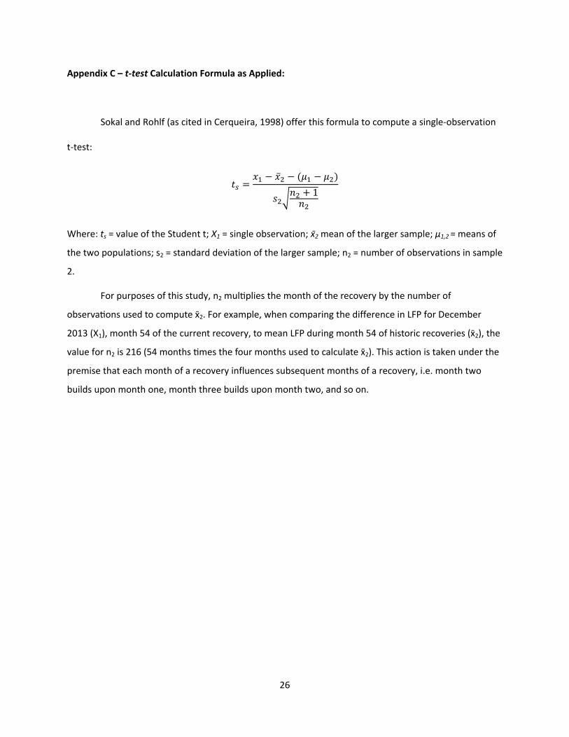
Appendix C – t‐test Calculation Formula as Applied:

Sokal and Rohlf (as cited in Cerqueira, 1998) offer this formula to compute a single‐observation

t‐test:

1

Where: ts = value of the Student t; X1 = single observation; x2 mean of the larger sample; µ1,2 = means of

the two populations; s2 = standard deviation of the larger sample; n2 = number of observations in sample

2.

For purposes of this study, n2 mul plies the month of the recovery by the number of

observa ons used to compute x2. For example, when comparing the difference in LFP for December

2013 (X1), month 54 of the current recovery, to mean LFP during month 54 of historic recoveries (x2), the

value for n2 is 216 (54 months mes the four months used to calculate x2). This action is taken under the

premise that each month of a recovery influences subsequent months of a recovery, i.e. month two

builds upon month one, month three builds upon month two, and so on.

27

Appendix D – LFP and Synthetic LFP Compared:

58%

60%

62%

64%

66%

68%

1973 1978 1983 1988 1993 1998 2003 2008 2013

LFP and Synthetic LFP 1973‐2013 rates, seasonally adjusted

Townsend, JGSPA; data source: BLS, June 20141Synthetic LFP detrends growth in female participation over 1973‐2013.

LFP

synthetic LFP1


28

Appendix E – Data Sources:

U.S. LFP

LFP represents the civilian labor force as a percentage of the civilian non‐institutional population.

Source: Bureau of Labor Statistics (BLS).

Ohio LFP

Source: Local Area Unemployment Statistics, BLS.

Synthetic LFP

Author’s calculations. Source: BLS.

Capacity Utilization

Capacity utilization is the percentage of resources used by corporations and factories to produce goods

in manufacturing, mining, and electric and gas utilities for all facilities located in the United States

(excluding those in U.S. territories). Source: Board of Governors of the Federal Reserve System.

Unemployment Rate

Seasonally adjusted. The unemployment rate represents the number of unemployed as a percentage of

the labor force. Source: BLS.

Disabled Worker Benefits Awarded

Source: Social Security Administration.

Unemployment Insurance, First Payments

Source: Employment & Training Administration.

2014 06 26 - Townsend White Paper - Recent Declines in Ohio US LFP

Documents

Transcript of 2014 06 26 - Townsend White Paper - Recent Declines in Ohio US LFP