Paper Author (s)

Daniel J. Fagnant (corresponding), University of Texas, Austin (danfagnant@hotmail.com)

Kara Kockelman, University of Texas, Austin (kkockelm@mail.utexas.edu)

Paper Title & Number

Simulating Fleet Operations for Shared Autonomous Vehicles Using Dynamic Ride Sharing in an Urban Network [ITM # 41]

Abstract

Carsharing programs that operate as short-term vehicle rentals (often for one-way trips before ending the rental) like Car2Go and ZipCar have quickly expanded, with the number of U.S. users growing from 12 thousand in 2002 to over 890 thousand by 2013. Such programs seek to shift personal transportation choices from an owned asset to a service used on demand. The advent of automated or fully self-driving vehicles will address many current carsharing barriers, including users’ travel to access available vehicles. This work describes the design of an agent-based model for Shared Autonomous Vehicle (SAV) operations, and the estimated travel impacts and environmental benefits of such settings, versus conventional vehicle ownership and use. Additionally, travelers are given the option of sharing SAV rides with others when the extra trip will add no more than 10% travel time to any shared trip. Four SAV relocation strategies are also implemented, in order to reduce traveler wait times. The model is applied in Austin, Texas and uses the region’s urban network and demographic settings to establish base trip-making patterns. Preliminary results indicate that each SAV can replace around ten conventional vehicles, but adds up to 10% more travel distance than comparable non-SAV trips. When dynamic ride sharing is implemented, total SAV-induced travel falls by 15%, rather than rising. This results in overall beneficial emissions impacts, particularly once fleet-efficiency changes and embodied versus in-use emissions are assessed.

Statement of Financial Interest

None

Statement of Innovation

This paper assesses the travel and environmental implications of shared autonomous vehicles using an agent-based simulation and incorporating dynamic ride sharing, modeled in an urban network setting.

DEVELOPMENT AND APPLICATION OF A NETWORK-BASED

SHARED AUTOMATED VEHICLE MODEL IN AUSTIN, TEXAS

Daniel J. Fagnant and Dr. Kara Kockelman

University of Texas at Austin

March 28, 2014

To be presented at the 2014 Transportation Research Board Conference on

Innovations in Travel Modeling, April 27-30 in Baltimore, MD

Word count: 6,830 (5,830 Words + 3 figures + 1 Table)

ABSTRACT

The emergence of self-driving vehicles holds great promise for the future of transportation.

While it will still be a number of years before fully self-driving vehicles can safely and legally

drive unoccupied on U.S. street, once this is possible, a new transportation mode for personal

travel looks set to arrive. This new mode is the shared automated vehicle (SAV), combining

features of short term rentals with the vehicles’ powerful automated self-driving capabilities.

This investigation examines SAVs’ potential implications at a low level of market penetration

(1.3% of regional trips) by simulating a fleet of SAVs serving travelers in Austin, Texas’ 12-mile

by 24-mile regional core. The simulation uses a synthetic population derived from the Capital

Area Metropolitan Planning Organization’s regional planning model trip tables to generate

demand across zone origins, destinations and departure times. CAMPO’s regional transportation

network is also used, with link-level travel times varying by time of day in response to

congestion, with average hourly travel speeds estimated using Nagel and Axhausen’s (2013)

MATSim agent-based dynamic traffic assignment simulation software.

Results show that each SAV is able to replace around 8.5 to 10 conventional vehicles while still

maintaining a reasonable level of service (as proxied by user wait times). Additionally,

approximately 18.5 to 20 percent more vehicle-miles traveled (VMT) may be generated, due to

SAVs journeying unoccupied to the next traveler, or relocating to a more favorable position in

anticipation of next-period demand.

INTRODUCTION

Vehicle automation appears poised to revolutionize the way in which we interface with the

transportation system. Google expects to introduce a self-driving vehicle by 2017 (O’Brien

2012), and multiple auto manufacturers including GM (LeBeau 2013), Mercedes Benz

(Andersson 2013), Nissan (2013) and Volvo (Carter 2012) are seeking to offer vehicles with

automated driving capabilities by 2020. While current regulations require a driver behind the

wheel to take control in case of an emergency even if the vehicle is operating itself, it is likely

that this requirement will fall away as further testing and demonstration proceeds apace, vehicle

automation technology continues to mature, and the regulatory environment adjusts. Once this

occurs, vehicles will be able to drive themselves even without a passenger in the car, opening the

door to a new transportation mode, the Shared Automated Vehicle (SAV).

SAVs merge the paradigms of short-term car rentals (as used with car sharing programs like

Car2Go and ZipCar), and taxi services (hence the alternative name of “aTaxis”, as coined by

Kornhauser et al. [2013]). The difference between the two frameworks is purely one of

perception and semantics: are SAVs short-term rentals of vehicles that drive themselves, or are

they taxis where the driver is the vehicle itself? The answer is both, and SAVs present a number

of potential advantages over both existing non-automated frameworks.

In relation to carsharing programs, SAVs have the capability to journey unoccupied to a waiting

traveler, thus obviating the need for continuing the rental while at their destination, or worrying

about whether a shared vehicle will be available when the traveler is ready to departing. Also,

SAVs possess advantage over non-automated shared vehicles in that they can preemptively

anticipate future demand and relocate in advance to better match vehicle supply and travel

demand. When comparing an SAV framework to regular taxis, Burns et al. (2013) estimated that

SAVs may be more cost effective on a per-mile basis than taxis operating in Manhattan, cutting

average trip costs from $7.80 to $1 due to the automation of costly human labor, though these

figures may be somewhat optimistic since their analysis assumed a low (marginal) cost of just

$2,500 for self-driving automation capabilities.

Given the distinct advantages that this emerging mode could hold over taxis and shared vehicles,

it is important to understand the possible implications and operation of SAVs, as they may

become a potentially significant share of personal travel in urban areas. This investigation does

exactly that, by modeling Austin, Texas travel patterns and anticipating SAV implications by

serving a small share of travelers who previously traveled using other modes (mostly private

automobile). This investigation is also unique among other SAV investigations to date (e.g.,

Fagnant and Kockelman [2014] Kornhauser et al. [2013], Burns et al. [2013], and Pavone et al.

[2011]) in that the analysis uses an actual transportation network, with link-level travel speeds

that vary by time of day, in response to differing levels of congestion.

THE AUSTIN NETWORK AND TRAVELER POPULATION

The base Austin regional network, zone system, and trip tables were obtained from the Capital

Area Metropolitan Planning Organization (CAMPO), and are used in CAMPO’s regional travel

demand modeling efforts. The network is structured around 2,258 traffic analysis zones (TAZs)

that define geospatial areas within the six-county Austin metropolitan region. A centroid node is

located at the geographic center of each TAZ, and all trips departing from or traveling to the

TAZ are assumed to originate from or end at this centroid. A set of centroid connectors link

these zone centroids to this rest of the Austin regional transportation network. The network

consists of 13,594 nodes and 32,272 links, including centroids and centroid connectors.

To determine SAV travel demand, a synthetic population of (one-way) trips was generated from

the region’s zone-based trip table, using four times of day: 6AM – 9AM for the morning peak,

9AM – 3:30PM for mid-day, 3:30PM – 6:30PM for an afternoon peak, and 6:30PM – 6AM for

night conditions. Each of these time of day periods are used to identify different levels of trip

generation and attraction between TAZs. Within each of these four broad periods, detailed trip

departure time curves or distributions were developed based on Seattle’s year-2006 household

travel diaries (PSRC 2006), since the Austin household travel survey data set’s departure times

did not make sense (e.g., the strongest demand during the PM peak was modeled at 3PM, as well

as other issues that rose questions about the representative nature of the departure time

distribution).

Once the trip population was generated, a full-weekday (24-hour) simulation of Austin’s

personal- and commercial-travel activities was conducted using the agent-based dynamic-traffic

simulation software MATsim (Nagel and Axhausen, 2013). This evaluation assumed a typical

weekday under current Austin conditions, using a base trip total of 5 million trips (per day),

including commercial-vehicle trips, with 0.5 million of the total trips coming from and/or ending

their travel outside the 6-county region. Outputs of the model run were generated, including

link-level hourly average travel times for all 24 hours of the day. Next, a 100,000 trip subset of

the trip population was selected using random draws, and the 57,161 travelers (1.3% of the total

internal regional trips, originating from 734 TAZ centroids) falling within a centrally located 12-

mile by 24-mile “geofence” were assumed to call on SAVs for their travel. This geofence area

was chosen because it represents the area with the highest trip density, and would therefore be

best suitable for SAV operation, in terms of both lower traveler wait times and less unoccupied

SAV travel as SAVs journey between one traveler drop-off to the next traveler pick-up. All trips

originating from or traveling to destinations outside the geofence were assumed to rely on

alternative travel modes (e.g., a rental car, privately owned car, bus, light-rail train, or taxi).

Figure 1a depicts the overall Austin regional network and geofence location, Figure 1b shows the

geofence area in greater detail, and Figure 1c shows the density of trip origins within the

geofence area, using half-mile resolution within 2-mile (outlined) blocks, with darker areas

representing higher trip-making intensities.

Figure 1: (a) Regional Transportation Network, (b) Nework within the 12 mi x 24 mi Geofence,

(c) Distribution of Trip Origins (over 24-hour day, at ½-mile resolution)

MODEL SPECIFICATION AND OPERATIONS

The population of trips within the geofenced area, the transportation network, and hourly link-

level travel times were then used to simulate how this subset of trips would be served by SAVs,

rather than using personally-owned household vehicles. This simulation was conducted by

loading network and trip characteristics into a new C++ coded program, and simulating the SAV

fleet’s travel operations over a 24-hour day. To accomplish this, four primary program sub-

modules were developed, including SAV location and trip assignment, SAV fleet generation,

SAV movement, and SAV relocation.

SAV Location and Trip Assignment

The SAV location module operates by determining which available SAVs are closest to waiting

travelers (prioritizing those who have been waiting longest), and then assigning available SAVs

to those trips. For each new traveler waiting for an SAV, the closest SAV is sought using a

backward-modified Dijkstra’s algorithm (Bell and Iida 1997). This ensures that the SAV that is

chosen has a shorter travel time to the waiting traveler than any other SAV that is not currently

occupied. A base maximum path time is set equal to 5 minutes, and, if an SAVs is located

within the desired time constraint, it will be assigned to the trip. Once an SAV has been assigned

to a traveler, a path is generated for the SAV, from its current location to the waiting traveler (if

the SAV and traveler are on different nodes) and then to the traveler’s destination. This is done

using a time-dependent version of Dijkstra’s algorithm, by tracking future arrival times at

individual nodes and corresponding link speeds emanating from those nodes at the arrival time.

Persons unable to find an available SAV within a 5-minute travel time are placed on a wait list.

These waiting persons expand their maximum SAV search radius to 10 minutes. The program

prioritizes those who have waiting the longest, serving these individuals first before looking for

SAVs for travelers who have been waiting a shorter time, or who have just placed a pick-up

request. As such, an SAV may be assigned to a traveler who has been waiting 10 minutes and is

8 minutes away from a free SAV over another traveler who has been waiting 5 minutes and is

just 2 minutes away from the same vehicle (provided that there are no closer SAVs to the first

traveler).

Another feature of the SAV search is a process by which the search area expands. First, travelers

look for free SAVs at their immediate node, then a distance of one minute away, then two

minutes, and so forth, until the maximum search distance is reached or a free SAV is located.

This is conducted to help ensure that vehicles will be assigned to the closest traveler, rather than

simply to the first traveler who looks within a given time-step interval.

SAV Fleet Generation

In order to assign an SAV to a trip, an SAV fleet must first exist. The fleet size is determined by

running a SAV “seed” simulation run, in which new SAVs are generated when any traveler has

waited for 10 minutes and is still unable to locate an available SAV within 10 minutes travel

time (i.e., if a vehicle does not free up in the next 5 minutes, the traveler must wait at least 20

minutes). In these instances, a new SAV is generated for the waiting traveler at his/her current

location and the SAV remains in the system for the rest of the day. At the end of the SAV seed

day, the entire SAV fleet is assumed to be in existence, and no new SAVs are created for the

next full day, for which the outcome results are measured and reported. All SAVs begin the

following day at the location in which they ended the seed day, reflecting the phenomenon that

each individual SAV will not always end up at or near the place where it began its day.

SAV Movement

Once an SAV is assigned to a traveler or given relocation instructions, it begins traveling on the

network. During this time the SAV follows the series of previously planned (shortest-path)

steps, tracking its position within the network, until 5 minutes of travel have elapsed or the SAV

has reached its final destination. Link-level travel speeds vary every hour, thanks to the

MATsim simulation results (using 5 percent of the original trip table, on a 5-percent capacity

network, to reduce computing burdens in this advanced, dynamic micro-simulation model).

SAVs also track the time to the next node on their path, so an SAV’s partial progress on a link is

saved at the end of the 5-minute time interval, to be continued at the start of the next time

interval. If an SAV arrives at a traveler, a pickup time cost of one minute is incurred before the

SAV continues on its path. Also, once an SAV arrives at the traveler’s destination, any

remainder of the five-minute interval is considered lost drop-off time, and the SAV cannot serve

another traveler or begin relocating until the start of the next five-minute interval.

SAV Relocation

While the SAV location, assignment, generation, and movement framework described above is

sufficient for basic operation of an SAV system, any SAV’s ability to relocate in response to

waiting travelers and the next (5-minute) period’s anticipated demand is important for improving

the overall system’s level of service. Using a similar grid-based model, Fagnant and Kockelman

(2014) tested four different SAV relocation strategies, alone, in combination, and in comparison

to a no-relocation strategy. These results showed how the most effective of the four strategies

evaluated the relative imbalance in number of waiting travelers and expected demand for trip-

making across 2-mile by 2-mile blocks, and then pulled SAVs from adjacent blocks if local-

block supply was too low in relation to expected demand, or pushed SAVs into neighboring

blocks if local supply greatly exceeded expected (next-period) demand. This resulted in

dramatic improvements in wait times, with the share of 5-minute wait intervals (incurred with

every 5-minute period a traveler waits for an SAV) falling by 82 percent (from 2422 to 433)

when using this strategy (versus no relocation strategy in place), even with slightly fewer SAVs.

This same block balancing strategy was implemented here, by first calculating a block balance

for each 2-mile by 2-mile block, using the following formula:

(

) (1)

This formula compares the share of SAVs within a given block to share of (expected, next-

period) total demand within the same block, normalizing by the total number of SAVs (or fleet

size). Therefore, the total block balance represents the excess or deficit number of SAVs within

the block in relation to system-wide SAV supply and expected travel demand. Expected travel

demand is calculated as waiting trips plus the expected number of new travelers that are likely to

request pickup and departure in the next five-minute interval. The number of new travelers is

estimated based by segmenting system-wide trips into one-hour bins, and obtaining average 5-

minute trip rates for each block. Any agency or firm operating a fleet of SAVs could probably

use historical demand data to inform their fleet’s relocation decisions.

Once block balances are assessed, the block with the greatest imbalance is chosen (i.e., the

greatest absolute value of Equation 1’s result). Those with balance values less than -5 will

attempt to pull available SAVs from neighboring blocks, first seeking to pull SAVs (if present)

from the surrounding blocks with the highest (positive) balance scores. If a block has a positive

balance above +5, it will similarly attempt to push SAVs into neighboring blocks with the lowest

balance scores. In both cases, the balance difference between blocks must be greater than 1 in

order to justify relocation.

After directions are assigned, the next task is to determine which individual SAVs to push or pull

into the neighboring blocks. This is done by conducting path searches to determine which SAVs

are closest to the node that is located nearest to the center of the block that the SAV will be

moving into. If a pushed SAV is closest to the central nodes in two or more blocks (for example,

5.5 minutes to the block immediately north and 7.4 minutes to the block immediately west), it

will be assigned to travel in the direction with the shortest path. These SAV paths are created

from their current locations to the central node in the destination block. Each path is then

trimmed after 5 minutes of relocation travel, such that the SAV can reassess its position and

potentially be assigned to an actual traveler. If it has entered the new block and has traveled at

least 2 minutes while in the new block in the direction of the central node, it will be held at that

position for a coming assignment; this halt on relocation towards the new block’s central node

helps ensure that too many pushed SAVs do not all end up at the central node.

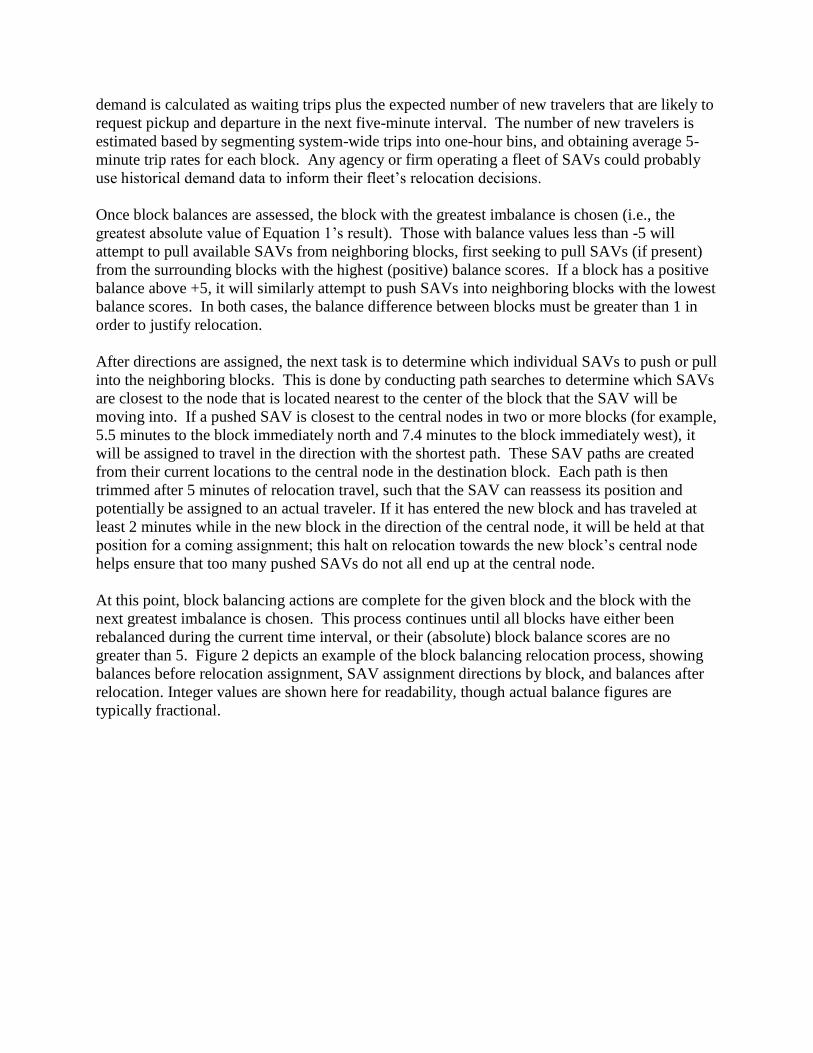
At this point, block balancing actions are complete for the given block and the block with the

next greatest imbalance is chosen. This process continues until all blocks have either been

rebalanced during the current time interval, or their (absolute) block balance scores are no

greater than 5. Figure 2 depicts an example of the block balancing relocation process, showing

balances before relocation assignment, SAV assignment directions by block, and balances after

relocation. Integer values are shown here for readability, though actual balance figures are

typically fractional.

Figure 2: Example SAV Relocations to Improve Balance in 2-mile Square Blocks (a) Initial

Expected Imbalances, (b) Directional SAV Block Shifts, and (c) Resulting Imbalances

The other three relocation strategies used by Fagnant and Kockelman (2014) are not used here.

They include a similar block-balance strategy, using 1-mile square blocks, relocation of extra

SAVs to quarter-mile grid cells with zero SAVs in them and surrounding them (and thus half-

mile travel distance away), and a stockpile-shifting strategy that relocates SAVs a quarter mile (1

grid cell away) if too many SAVs are present at a given location relative to the immediately

surrounding cells (i.e., local imbalances of 3 of more in available SAVs). While these other

strategies were somewhat helpful in reducing delays, their overall impact was less than that of

the 2-mile-block rebalancing strategy, even when all three were combined. Moreover, the latter

two strategies (involving very local or myopic shifts) may not be as effective in the more realistic

network setting modeled here, since not every cell is a potential trip generator here, and

differences in nearby trip-generation rates can vary dramatically across adjacent Austin cells. In

this Austin setting, while only one of the 72 two-mile by two-mile blocks had no simulated SAV

demand, 43.7 percent of the half-mile by half-mile cells had demand (with demand originating

from an average of 1.46 centroids per non-zero-demand cell). Moreover, among the 503 half-

mile cells exhibiting some demand, the cumulative trips generated in such cells may be more

than 10 times as many as in any adjacent cell.

MODEL APPLICATION AND RESULTS

The model was tested using more than 57% of the randomly selected 100,000 trips in the Austin

regional (6-county) trip table that contained both origins and destinations within the 12 x 24 mile

geofence, and given departure times to mimic a natural 24-hour cycle of trips (as described

earlier). The spatial pattern of these trips’ origins is shown earlier, in Figure 1c. This single day

was then run to generate a fleet of SAVs (to ensure wait times were below 10 minutes), and then

a subsequent day was run using the same trip population to examine travel implications of the

operating SAV fleet. These results show how approximately 2,217 SAVs are needed to serve the

sample of trips, so that each SAV serves an average of 25.6 trips on the single simulated day.

Assuming an average of 3.02 trips per day per licensed driver and 0.99 licensed drivers per

conventional vehicle, an SAV in this scenario could reasonably be expected to replace around

8.40 conventional vehicles.

This SAV fleet size also offers an excellent level of service: Average wait times throughout the

day are modeled to be less than 50 seconds, with 96.2% of travelers waiting less than 5 minutes,

99.5% of travelers waiting under 10 minutes, and less than 0.01% of travelers waiting 15-19

minutes. The highest average wait times occurred during the 5PM – 6PM hour, when demand

was highest and speeds slowest/congestion worst, with average wait times just over 2 minutes

(assuming that travelers call on 5-minute cycles, so some may want to call before that horizon,

adding on average another 2.5 minutes to the expected wait time since trip request).

Additionally, it should be noted that some travelers may wish to call many minutes or hours in

advance of needing an SAV, though these results suggest that such reservations may not be too

helpful, except perhaps in lower-density and/or harder-to-reach locations. Indeed, in some cases

this may make the system operate worse if the person who placed the call is not ready and the

SAV could be serving another traveler, particularly during high demand times.

While this paradigm appears socially beneficial in terms of replacing many conventional vehicles

with a much smaller fleet of SAVs, it comes with some costs in terms of extra, (empty-) vehicle-

miles traveled (VMT). SAVs are estimated to travel another 18.5 percent distance without

occupants, and all this extra VMT is not likely to occur if travelers are driving their own cars. Of

course, many conventional-vehicle travelers do pass their destinations to find a parking place

(and many may spend a lot of time and distance searching for a space on the street or within a

structured parking lot). For example, Shoup (2007) estimated such “cruising for parking” to

constitute 30 percent of VMT traveled in some of the world’s busiest downtowns. This extra

VMT stems from SAVs traveling unoccupied to pick up the next waiting traveler, and from

SAVs relocating between blocks in response to current and anticipated future demand. When the

relocation process was removed, the empty-VMT share fell to 15.8%, though average wait times

grew by 57% (from 0.81 min to 1.27 min), and the share of travelers waiting 10 minutes or more

grew from 0.50% of travelers to 1.78%.

Other system simulation results of note are average 24-hour travel-distance-weighted speeds of

41.1 mph. However, when taking a time-weighted system perspective of total travel distance

divided by total travel miles (VMT/VHT), average system speeds fall to 25.6 mph. This reflects

the phenomenon that if a given SAV travels 5 miles at 5 mph and 5 miles at 50 mph, it will take

1.1 hours to travel the 10 miles resulting in an effective system speed of 9.1 mph, rather than a

travel-distance weighted speed of 27.5 mph. 22.2% of total miles traveled were at slow speeds at

or below 20 mph, likely on local roads or during congested times, and 35.9% of total miles

traveled over 50 mph, typically during off-peak times on freeways.

It is also informative to assess the potential charging implications for an electric SAV fleet, as

investigated (for cost comparisons, but not vehicle charging) by Burns et al. (2013). Occupied

trip distances average 4.78 miles, and the SAV fleet was traveling, picking up, dropping off, or

otherwise active for 7.75 hours of the day, with SAVs averaging 3.22 stationary intervals of at

least one hour when no travelers were being served, and another 2.25 intervals between 30

minutes and 55 minutes. Additionally, daily travel distances averaged 149 miles of travel per

SAV, with mileage distributions shown in Figure 3.

Figure 3: Daily travel distance per SAV

Among currently available battery-electric (non-hybrid) vehicles for sale in the U.S., the US

EPA (2014) notes that charge times to fully charge a battery typically vary between 4 and 7

hours on 240 Volt Level 2 charging devices, with all-electric ranges between 60 and 100 miles.

This could pose a serious issue for all-electric BEVs in an SAV fleet, but not much of an issue

for plug-in hybrid EVs, fast-charging settings (480-volt, Level 3), or the Tesla Model S (which is

a BEV with 208 to 265 mile range and a charge time of under 5 hours when using a dual

charger). Of course, many years are required to develop the automation technology and legal

framework required to successfully deploy SAVs, and battery charging times, ranges and costs

will improve, along with deployment of fast-charging facilities – and remote charging devices (to

allow for self-charging of AVs).

Following the base model’s simulation run, a series of different SAV fleet size limitations were

imposed, to appreciate the wait-time and empty-VMT implications of using fewer vehicles to

serve the same number of trips. The fleet size was reduced in increments of 100 SAVs, from the

base SAV fleet size of 2217 to a low-end fleet size of just 1817 vehicles, with each scenario

serving 57,161 trips over a 24-hour period in the 12 mi x 24 mi sub-region. Fagnant and

Kockelman’s (2014) idealized 10 mi x 10 mi quarter-mile grid-based-system results are also

included here (with 60,551 travelers served), for comparison purposes.

Table 1: Model results under different SAV fleet sizes

Scenario 2217 SAVs 2117 SAVs 2017 SAVs 1917 SAVs 1817 SAVs

Grid-

based*

Conventional vehicle

replacement 8.45 8.85 9.29 9.77 10.31 11.76

Average traveler wait

time 48.5 sec 58.1 sec 71.2 sec 97.0 sec 144.5 sec 17.7 sec

% of travelers waiting

10+ min 0.50% 0.74% 1.21% 3.43% 9.08% 0.006%

% of empty

(unoccupied) VMT 18.5% 18.6% 18.8% 19.3% 20.2% 10.7%

*10-mile by 10-mile idealized-context grid-based simulation can be found in Fagnant and Kockelman (2014).

0

100

200

300

400

500

600

700

# o

f SA

Vs

Miles traveled in one day

From this evaluation it appears that a relatively high level of service may be maintained with 5 to

15 percent lower SAV fleet sizes. Even when reducing the fleet size by 18%, to just 1817 SAVs

(serving 60,551 trips per day), average wait times remain under two and a half minutes. This is

probably competitive with -- or better than -- walk times to parking spots and/or transit stops for

most travelers. The most obvious level of service impacts are not in terms of average wait times,

but in the share of travelers waiting for longer periods of ten minutes or more. Long wait times

may discourage SAV usage, particularly if these wait times consistently occur during the time an

individual usually wishes to travel. For example, in the 1817-SAV scenario, travelers departing

between 5 and 6 PM experienced an 8.62 minute average wait. This could push a number of

persons who regularly travel during this time to drive themselves instead of relying on SAVs,

pay a premium for faster service, and/or simply share rides in these SAVs.

Fortunately, the share of unoccupied travel increases very little with smaller SAV fleets: rising

from 18.5 to 20.2 percent as fleet size falls 18 percent, from 2217 to 1817 SAVs. (The direction

of this effect is intuitive, since fewer SAVs will be close at hand, to serve trip demands that

emerge.)

It is also interesting to compare the results shown here with the grid-based evaluation results

provided by Fagnant and Kockelman (2014) for a symmetric 10-mile by 10-mile setting. Their

pure-grid scenario with quarter-mile cells and smooth (idealized) demand profiles out-performs

the much more realistic, actual-network-based Austin scenario, across all categories of

conventional vehicle replacement, wait times, and unoccupied travel. Their grid-based

evaluation found that each SAV could replace three more conventional vehicles than this more

realistic setting, while cutting average wait times nearly 67% and with 42% less unoccupied

VMT. The differences in these two application results come from a host of very different

supporting assumptions.

First, the travel demand profile differed significantly between the two evaluations. The grid-

based evaluation assumed a smaller service area and higher trip density, with 60,551 trips per

day across a 100 square-mile area, versus 57,161 trips per day in a 288 square-mile area.

Average trip-end intensities also varied quite smoothly across quarter-mile cells in the grid-based

application (with near-linear changes in travel demand rates between the city center and the outer

periphery), whereas the Austin setting exhibits much greater spatial variations in trip-making

intensities (as evident in Figure 1c). The simulated setting also added more fleet vehicles based

on initial simulations, to keep wait times lower than would probably be optimal for real fleet

managers; this Austin fleet sizing is less generous, and presumably more realistic, but traveler

wait times remain very reasonable.

Another key distinction between the simulated, grid-based and Austin network evaluations

emerges in average speeds and average trip distances. Here, travel-weighted 24-hour running

speeds average 21.3 mph, whereas constant speeds of 21 mph and 33 mph were assumed in the

simulated context, and the 21 mph speed only applied during a 1-hour AM peak and 2.5-hour

PM peak period (with 33 mph SAV travel speeds at all other times). Trip distances in the

simulated setting were also higher, averaging 5.43 miles in contrast to shorter 4.87 mile average

trip distance in the network-based evaluation. However, trips were constrained to 15 miles in

length in the prior application, while this application permits a much wider range of travel

behaviors. Finally, this setting allows for a real network – sometimes dense, but often sparse,

adding circuity to travel routes; in contrast, the simulated setting assumed a tightly space

(quarter-mile) grid of north-south and east-west streets throughout the region. Circuity in

accessing travelers and then their destinations is harder to serve, especially at lower average

speeds, across a wider range of trip-making intensities.

It is interesting how well the Austin fleet still serves its travelers, given the series of

disadvantages that exist in this more realistic simulation. Lower trip densities mean that SAVs

must travel farther on average to pick up travelers, and slower speeds mean that SAVs will be

occupied for a longer duration during the journey, tying them up and preventing them from

serving other travelers, and potentially hampering relocation efficiency. Also, while shorter trips

lessen travel times, it also means that relocation and unoccupied travel will comprise a greater

share of the total. All of these factors suggest that a larger fleet will be needed to achieve an

equivalent level of service. But the vehicle-replacement rates remain strong, at 8 or more

conventional vehicles per SAV.

CONCLUSIONS

These Austin-based simulation results suggest that a fleet of SAVs could serve many if not all

intra-urban trips with replacement rates of 1 SAV per 8.5 to 10 conventional vehicles (depending

on desired level of service), though in the process SAVs may generate 18.5 to 20 percent new

unoccupied/empty-vehicle travel that would not exist if travelers were driving their own

vehicles. Prior results by Fagnant and Kockelman (2014) indicate that as demand intensity (over

space) for SAV travel increases, the number of conventional vehicles that each SAV can replace

grows, wait times fall, and unoccupied travel distances fall. All this points to a high cost per

SAV in the early stages of deployment (in terms of new VMT), though such costs should fall in

the long term, as larger SAV fleet sizes lead to greater efficiency. Also, other potential

synergistic opportunities exist in combination with SAVs like dynamic ride sharing (e.g.,

Kornhauser et al. [2013]) that may counterbalance the negative impacts of new VMT through

unoccupied travel.

Moreover, these results have substantial implications for parking and emissions. For example, if

an SAV fleet is sized to replace 9.0 conventional vehicles for every SAV, total parking demand

will fall by around 8 vehicle spaces per SAV (or possibly more, since the vehicles are largely in

use during the daytime). These spaces would free up parking supply for privately held vehicles

or other land uses. In this way, the land and costs of parking provision could shift to better uses,

like parks and retail establishments, offices, wider sidewalks, bus parking, and bike lanes.

With regards to vehicle emissions and air quality, many benefits may exist, even in the face of 20

percent higher VMTs. For example, SAVs may be purpose-built as a fleet of passenger cars,

replacing many current, heavier vehicles with higher emissions rates (like pickup trucks, SUVs

and passenger vans). SAVs will also be traveling much more frequently throughout the day than

conventional vehicles (averaging 30 trips per day rather than 3, for example, and in use 7.75

hr/day, rather than 1 hour), so they will have many fewer cold starts than the vehicles they are

replacing. Cost-start emissions are much higher than after a vehicle’s catalytic converter has

warmed up, and these results suggest 5.4 times fewer cold starts (defined as rest periods greater

than 1 hour), when replacing conventional, privately held vehicles with SAVs.

Finally, SAVs hold great promise for harnessing vehicle automation technology, with features of

high utilization rates and quick turnover. By using SAVs intensely (results here show around

149 miles per SAV per day, or 54.3 thousand miles per year), they will presumably wear out and

need replacement every two to three years. Since vehicle automation technology is evolving

rapidly, this cycling will allow fleet operators to consistently provide SAVs with the latest

sensors, actuation controls, and other automation hardware, which tends to be much more

difficult to provide than simple SAV system firmware and software updates.

In summary, while the future remains uncertain, these results indicate that SAVs may become a

very attractive option for personal travel. Each SAV has the potential to replace many

conventional vehicles, freeing up parking and leading to more efficient household personal

vehicle ownership choices. Though extra VMT through unoccupied travel is a potential

downside, vehicle fleet changes, a reduction in cold-starts, and dynamic ride sharing may be able

to counteract these negative impacts and lead to net beneficial environmental outcomes.

REFERENCES

Andersson, Leif Hans Daniel. 2013. Autonomous Vehicles from Mercedes-Benz, Google, Nissan

by 2020. The Dish Daily. November 22.

Bell, M. G. and Iida, Y, 1997. Transportation Network Analysis. John Wiley & Sons. New York.

Burns, Lawrence, Jordan, William, Scarborough, Bonnie. 2013. Transforming Personal Mobility.

The Earth Institute – Columbia University, New York.

Carter, Marc. 2012. Volvo Developing Accident-Avoiding Self-Driving Cars for the Year 2020.

Inhabitat. December 5.

Fagnant, Daniel and Kockelman, Kara. 2014. Environmental Implications for Autonomous

Shared Vehicles Using Agent-Based Model Scenarios. Transportation Part C 40:1-13.

LeBeau, Philip. 2013. General Motors on Track to Sell Self-Driving Cars. 7 October, CNBC.

Kornhauser, A., Chang A., Clark C., Gao J., Korac D., Lebowitz B., Swoboda A. 2013.

Uncongested Mobility for All: New Jersey’s Area-wide aTaxi System. Princeton University.

Princeton, New Jersey.

Nagel, Kai and Axhausen, Kay. 2013. MATSim: Multi-Agent Transport Simulation. Version 5.0.

http://www.matsim.org.

Nissan Motor Company. 2013. Nissan Announces Unprecedented Autonomous Drive

Benchmarks [Press Release]. http://nissannews.com/en-US/nissan/usa/releases/nissan-

announces-unprecedented-autonomous-drive-benchmarks.

Pavone, M., S. Smith, E. Frazzoli, and D. Rus. 2011. Load Balancing for Mobility-on-Demand

Systems. Robotics: Science and Systems Online Proceedings 7.

Puget Sound Regional Council. 2006. 2006 Household Activity Survey. Seattle, WA.

http://psrc.org/data/surveys/2006-household/.

Shoup, Donald. 2007. Cruising for parking. Access 30, 16–22.

United States Environmental Protection Agency. 2014. All-Electric Vehicles: Compare Side-By-

Side. http://www.fueleconomy.gov/feg/evsbs.shtml.