Pairwise MRF Calibration by Perturbation of the … · Pairwise MRF Calibration by Perturbation of...
39
HAL Id: hal-00743334 https://hal.inria.fr/hal-00743334 Submitted on 18 Oct 2012 HAL is a multi-disciplinary open access archive for the deposit and dissemination of sci- entific research documents, whether they are pub- lished or not. The documents may come from teaching and research institutions in France or abroad, or from public or private research centers. L’archive ouverte pluridisciplinaire HAL, est destinée au dépôt et à la diffusion de documents scientifiques de niveau recherche, publiés ou non, émanant des établissements d’enseignement et de recherche français ou étrangers, des laboratoires publics ou privés. Pairwise MRF Calibration by Perturbation of the Bethe Reference Point Cyril Furtlehner, Yufei Han, Jean-Marc Lasgouttes, Victorin Martin To cite this version: Cyril Furtlehner, Yufei Han, Jean-Marc Lasgouttes, Victorin Martin. Pairwise MRF Calibration by Perturbation of the Bethe Reference Point. [Research Report] RR-8059, INRIA. 2012, pp.35. <hal- 00743334>
-
Upload
truongtuyen -
Category
Documents
-
view
219 -
download
0
Transcript of Pairwise MRF Calibration by Perturbation of the … · Pairwise MRF Calibration by Perturbation of...
HAL Id: hal-00743334https://hal.inria.fr/hal-00743334
Submitted on 18 Oct 2012
HAL is a multi-disciplinary open accessarchive for the deposit and dissemination of sci-entific research documents, whether they are pub-lished or not. The documents may come fromteaching and research institutions in France orabroad, or from public or private research centers.
L’archive ouverte pluridisciplinaire HAL, estdestinée au dépôt et à la diffusion de documentsscientifiques de niveau recherche, publiés ou non,émanant des établissements d’enseignement et derecherche français ou étrangers, des laboratoirespublics ou privés.
Pairwise MRF Calibration by Perturbation of the BetheReference Point
Cyril Furtlehner, Yufei Han, Jean-Marc Lasgouttes, Victorin Martin
To cite this version:Cyril Furtlehner, Yufei Han, Jean-Marc Lasgouttes, Victorin Martin. Pairwise MRF Calibration byPerturbation of the Bethe Reference Point. [Research Report] RR-8059, INRIA. 2012, pp.35. <hal-00743334>

ISS
N0
24
9-6
39
9IS
RN
INR
IA/R
R--
80
59
--F
R+
EN
G
RESEARCH
REPORT
N° 80592012
Project-Teams TAO and Imara
Pairwise MRF
Calibration by
Perturbation of the Bethe
Reference Point
Cyril Furtlehner, Yufei Han, Jean-Marc Lasgouttes, Victorin Martin

RESEARCH CENTRE
SACLAY – ÎLE-DE-FRANCE
Parc Orsay Université
4 rue Jacques Monod
91893 Orsay Cedex
Pairwise MRF Calibration by Perturbation of
the Bethe Reference Point
Cyril Furtlehner∗, Yufei Han†, Jean-Marc Lasgouttes†, VictorinMartin∗
Project-Teams TAO and Imara
Research Report n° 8059 — 2012 — 35 pages
Abstract: We investigate different ways of generating approximate solutions to the inverseproblem of pairwise Markov random field (MRF) model learning. We focus mainly on the in-verse Ising problem, but discuss also the somewhat related inverse Gaussian problem. In bothcases, the belief propagation algorithm can be used in closed form to perform inference tasks. Ourapproach consists in taking the Bethe mean-field solution as a reference point for further perturba-tion procedures. We remark indeed that both the natural gradient and the best link to be addedto a maximum spanning tree (MST) solution can be computed analytically. These observationsopen the way to many possible algorithms, able to find approximate sparse solutions compatiblewith belief propagation inference procedures. Experimental tests on various datasets with refinedL0 or L1 regularization procedures indicate that this approach may be a competitive and usefulalternative to existing ones.
Key-words: Random Markov Fields, Ising Models, Inference, inverse problem, mean-field,beliefpropagation)
∗ Inria Saclay† Inria Paris-Rocquencourt

Calibration de Champ Markovien Aléatoire par
Perturbation de la Solution de Bethe
Résumé : Nous étudions différentes méthodes pour trouver des solutions approchées au prob-lème inverse de calibration de champ Markovien aléatoire à interaction de paires. Nous consid-érons principalement au modèle d’Ising ainsi qu’au problème lié de modèle Gaussien. En principedans ces deux cas l’algorithme de propagation de croyance peut-être utilisé sous forme cohérentepour résoudre des problèmes d’inférence. Notre approche consiste à utiliser la solution de champmoyen de Bethe comme référence et d’effectuer différentes perturbations à partir de ce pointde départ. Nous remarquons en particulier que le gradient naturel ainsi que le lien optimal àajouter a graphe de facteurs obtenu comme arbre couvrant maximal peuvent être obtenus defaçon analytique. Ces observation ouvrent un certain nombre de perspectives algorithmiquespermettant de trouver des solutions sur des graphes dilués, compatibles avec la propagation decroyances. Des tests numériques portant sur différents jeux de données permettant une com-paraison à des methodes de régularisation L0 ou L1 indiquent que cette approche peut-être unealternative compétitive aux méthodes classiques.
Mots-clés : Champs Markovien aléatoires, modèle d’Ising, Inférence, problème inverse, champmoyen, propagation de croyances
Pairwise MRF Calibration 3
Contents
1 Introduction 3
2 Preliminaries 42.1 Inverse Ising problem . . . . . . . . . . . . . . . . . . . . . . . . . . . . . . . . . . 42.2 More on the Bethe susceptibility . . . . . . . . . . . . . . . . . . . . . . . . . . . 102.3 Sparse inverse estimation of covariance matrix . . . . . . . . . . . . . . . . . . . . 12
3 Link selection at the Bethe point 143.1 Bethe approximation and Graph selection . . . . . . . . . . . . . . . . . . . . . . 143.2 Optimal 1-link correction to the Bethe point . . . . . . . . . . . . . . . . . . . . . 153.3 Imposing walk-summability . . . . . . . . . . . . . . . . . . . . . . . . . . . . . . 193.4 Greedy Graph construction Algorithms . . . . . . . . . . . . . . . . . . . . . . . . 21
4 Perturbation theory near the Bethe point 224.1 Linear response of the Bethe reference point . . . . . . . . . . . . . . . . . . . . . 224.2 Line search along the natural gradient in a reduced space . . . . . . . . . . . . . 234.3 Reference point at low temperature . . . . . . . . . . . . . . . . . . . . . . . . . . 24
5 L0 norm penalized sparse inverse estimation algorithm 25
6 Experiments 28
7 Conclusion 33
1 Introduction
The problem at stake is a model selection problem, in the MRF families, where N variablesare observed pair by pair. The optimal solution is the MRF with maximal entropy obeyingmoment constraints. For binary variables, this happens then to be the Ising model with highestlog-likelihood. It is a difficult problem, where both the graph structure and the value of the fieldsand coupling have to be found. In addition, we wish to ensure that the model is compatible withthe fast inference algorithm “belief propagation” (BP) to be useful at large scale for real-timeinference tasks. This leads us to look at least for a good trade-off between likelihood and sparsity.
Concerning the Inverse Ising Problem (IIP), the existing approaches fall mainly in the fol-lowing categories:
• Purely computational efficient approaches rely on various optimization schemes of the loglikelihood [21] or on pseudo-likelihood [18] along with sparsity constraints to select the onlyrelevant features.
• Common analytical approaches are based on the Plefka expansion [33] of the Gibbs freeenergy by making the assumption that the coupling constants Jij are small. The pictureis then of a weakly correlated uni-modal probability measure. For example, the recentapproach proposed in [7] is based on this assumption.
• Another possibility is to assume that relevant coupling Jij have locally a tree-like structure.The Bethe approximation [37] can then be used with possibly loop corrections. Again thiscorresponds to having a weakly correlated uni-modal probability measure and these kind ofapproaches are referred as pseudo-moment matching methods in the literature for the reason
RR n° 8059
4 Furtlehner & Han & others
explained in the previous section. For example the approaches proposed in [24, 35, 28, 36]are based on this assumption.
• In the case where a multi-modal distribution is expected, then a model with many attractionbasins is to be found and Hopfield-like models [19, 8] are likely to be more relevant. To bementioned also is a recent mean-field methods [32] which allows one to find in some simplecases the Ising couplings of a low temperature model, i.e. displaying multiple probabilisticmodes.
On the side of inverse Gaussian problem, not surprisingly similar methods have been developed byexplicit performing L0 and L1 matrix norm penalizations on the inverse covariance matrices, soas to determine sparse non-zero couplings in estimated inverse covariance matrices for large-scalestatistical inference applications [13, 20] where direct inversion is not amenable. In our contextthe goal is a bit different. In general cases, the underlying inverse covariance matrix is not neces-sarily sparse. What we aim to find is a good sparse approximation to the exact inverse covariancematrix. Furthermore, sparsity constraint is not enough for constructing graph structure that isused in conjunction with BP, known sufficient conditions referred as walk-summability [26] (WS)are likely to be imposed instead of (or in addition to) the sparsity constraint. To the best of ourknowledge not much work taking this point into consideration at the noticeable exception of [2]by restricting the class of learned graph structures. To complete this overview, let us mentionalso that some authors proposed information based structure learning methods [30] quite in linewith some approaches to be discussed in the present paper.
In some preceding work dealing with a road traffic inference application, with large scale andreal time specifications [16, 15, 14], we have noticed that these methods could not be used blindlywithout drastic adjustment, in particular to be compatible with belief propagation. This led usto develop some heuristic models related to the Bethe approximation. The present work is anattempt to give a theoretical basis and firmer ground to these heuristics.
2 Preliminaries
2.1 Inverse Ising problem
In this section we consider binary variables (xi ∈ 0, 1), which at our convenience may bealso written as spin variables si = 2xi − 1 ∈ −1, 1. We assume that from a set of historicalobservations, the empirical mean mi (resp. covariance χij) is given for each variable si (resp. eachpair of variable (si, sj)). In this case, from Jayne’s maximum entropy principle [23], imposingthese moments to the joint distribution leads to a model pertaining to the exponential family,the so-called Ising model:
P(s) =1
Z[J,h]exp
(
∑
i
hisi +∑
i,j
Jijsisj)
(2.1)
where the local fields h = hi and the coupling constants J = Jij are the Lagrange multipliersassociated respectively to mean and covariance constraints when maximizing the entropy of P.They are obtained as minimizers of the dual optimization problem, namely
(h⋆,J⋆) = argmin(h,J)
L[h,J], (2.2)
withL[h,J] = logZ[h,J] −
∑
i
himi −∑
ij
Jijmij (2.3)
Inria
Pairwise MRF Calibration 5
the log likelihood. This leads to invert the linear response equations:
∂ logZ
∂hi[h,J] = mi (2.4)
∂ logZ
∂Jij[h,J] = mij , (2.5)
mij = mimj + χij being the empirical expectation of sisj . As noted e.g. in [7], the solution is
minimizing the cross entropy, a Kullback-Leibler distance between the empirical distribution Pbased on historical data and the Ising model:
DKL[P‖P] = logZ[h,J] −∑
i
himi −∑
i<j
Jijmij − S(P). (2.6)
The set of equations (2.4,2.5) cannot be solved exactly in general because the computationalcost of Z is exponential. Approximations resorting to various mean field methods can be usedto evaluate Z[h,J].
Plefka’s expansion To simplify the problem, it is customary to make use of the Gibbs freeenergy, i.e. the Legendre transform of the free energy, to impose the individual expectationsm = mi for each variable:
G[m,J] = hT (m)m + F [h(m),J]
(with F [h,J]def
= − logZ[h,J], hTm is the ordinary scalar product) where h(m) depends implic-
itly on m through the set of constraints
∂F
∂hi= −mi. (2.7)
Note that by duality we have∂G
∂mi= hi(m), (2.8)
and[ ∂2G
∂mi∂mj
]
=
ïdh
dm
ò
ij
=
ïdm
dh
ò−1
ij
= −[ ∂2F
∂hi∂hj
]−1
=[
χ−1]
ij. (2.9)
i.e. the inverse susceptibility matrix. Finding a set of Jij satisfying this last relation along with(2.8) yields a solution to the inverse Ising problem since the m’s and χ’s are given. Still a wayto connect the couplings directly with the covariance matrix is given by the relation
∂G
∂Jij= −mij . (2.10)
The Plefka expansion is used to expand the Gibbs free energy in power of the coupling Jijassumed to be small. Multiplying all coupling Jij by α yields the following cluster expansion:
G[m, αJ] = hT (m, α)m + F [h(m, α), αJ] (2.11)
= G0[m] +∞∑
n=0
αn
n!Gn[m,J] (2.12)
RR n° 8059

6 Furtlehner & Han & others
where each term Gn corresponds to cluster contributions of size n in the number of links Jijinvolved, and h(m, α) depends implicitly on α in order to always fulfill (2.7). This preciselyis the Plefka expansion, and each term of the expansion (2.12) can be obtained by successivederivation of (2.11). We have
G0[m] =∑
i
1 +mi
2log
1 +mi
2+
1 −mi
2log
1 −mi
2.
Letting
HJdef
=∑
i<j
Jijsisj ,
using (2.7), the two first derivatives of (2.11) w.r.t α read
dG[m, αJ]
dα= −Eα
(
HJ
)
, (2.13)
d2G[m, αJ]
dα2= −Varα
(
HJ
)
−∑
i
dhi(m, α)
dαCovα
(
HJ , si)
, (2.14)
where subscript α indicates that expectations, variance and covariance are taken at given α. Toget successive derivatives of h(m, α) one can use (2.8). Another possibility is to express the factthat m is fixed,
dmi
dα= 0 = − d
dα
∂F [h(α), αJ]
∂hi
=∑
j
h′j(α) Covα(si, sj) + Covα(HJ , si),
giving
h′i(α) = −∑
j
[χ−1α ]ij Covα(HJ , sj), (2.15)
where χα is the susceptibility delivered by the model when α 6= 0. To get the first two terms inthe Plefka expansion, we need to compute these quantities at α = 0:
Var(
HJ
)
=∑
i<k,j
JijJjkmimk(1 −m2j ) +
∑
i<j
J2ij(1 −m2
im2j ),
Cov(
HJ , si)
=∑
j
Jijmj(1 −m2i ),
h′i(0) = −∑
j
Jijmj ,
(by convention Jii = 0 in these sums). The first and second orders then finally read:
G1[m,J] = −∑
i<j
Jijmimj , G2[m,J] = −∑
i<j
J2ij(1 −m2
i )(1 −m2j ),
and correspond respectively to the mean field and to the TAP approximation. Higher orderterms have been computed in [17].
Inria

Pairwise MRF Calibration 7
At this point we are in position to find an approximate solution to the inverse Ising problem,either by inverting equation (2.9) or (2.10). To get a solution at a given order n in the coupling,solving (2.10) requires G at order n+ 1, while it is needed at order n in (2.9).
Taking the expression of G up to second order gives
∂G
∂Jij= −mimj − Jij(1 −m2
i )(1 −m2j ),
and (2.10) leads directly to the basic mean-field solution:
JMFij =
χij(1 − m2
i )(1 − m2j ). (2.16)
At this level of approximation for G, using (2.8) we also have
hi =1
2log
1 +mi
1 −mi−
∑
j
Jijmj +∑
j
J2ijmi(1 −m2
j )
which corresponds precisely to the TAP equations. Using now (2.9) gives
∂hi∂mj
= [χ−1]ij = δij( 1
1 −m2i
+∑
k
J2ik(1 −m2
k))
− Jij − 2J2ijmimj .
Ignoring the diagonal terms, the TAP solution is conveniently expressed in terms of the inverseempirical susceptibility,
JTAPij = − 2[χ−1]ij
1 +√
1 − 8mimj [χ−1]ij, (2.17)
where the branch corresponding to a vanishing coupling in the limit of small correlation i.e. smallχij and [χ−1]ij for i 6= j, has been chosen.
Bethe approximate solution When the graph formed by the pairs (i, j) for which the cor-relations χij are given by some observations is a tree, the following form of the joint probabilitycorresponding to the Bethe approximation:
P(x) =∏
i<j
pij(xi, xj)
p(xi)p(xj)
∏
i
pi(xi), (2.18)
yields actually an exact solution to the inverse problem (2.2), where the p are the single and pairvariables empirical marginal given by the observations. Using the following identity
logpij(si, sj)
pi(si)pj(sj)=
(1 + si)(1 + sj)
2log
p11ij
p1i p
1j
+(1 + si)(1 − sj)
2log
p10ij
p1i p
0j
+(1 − si)(1 + sj)
2log
p01ij
p0i p
1j
+(1 − si)(1 − sj)
2log
p00ij
p0i p
0j
where the following parametrization of the p’s
pxidef
= p(1 + si
2= x
)
=1
2(1 + mi(2x− 1)), (2.19)
pxyijdef
= p(1 + si
2= x,
1 + sj2
= y)
=1
4(1 + mi(2x− 1) + mj(2y − 1) + mij(2x− 1)(2y − 1) (2.20)
RR n° 8059

8 Furtlehner & Han & others
relating the empirical frequency statistics to the empirical “magnetizations” m ≡ m, can be used.Summing up the different terms gives us the mapping onto an Ising model (2.1) with
hi =1 − di
2log
p1i
p0i
+1
4
∑
j∈∂i
log( p11
ij p10ij
p01ij p
00ij
)
, (2.21)
Jij =1
4log
( p11ij p
00ij
p01ij p
10ij
)
, ∀ (i, j) ∈ E , (2.22)
where di is the number of neighbors of i, using the notation j ∈ ∂i for “j neighbor of i”. Thepartition function is then explicitly given by
ZBethe[p] = exp
ï−1
4
∑
(i,j)∈E
log(
p00ij p
01ij p
10ij p
11ij
)
−∑
i
1 − di2
log(p0i p
1i )
ò(2.23)
The corresponding Gibbs free energy can then be written explicitly using (2.21–2.23). With fixedmagnetizations mi’s, and given a set of couplings Jij, the parameters mij are implicit function
mij = mij(mi,mj , Jij),
obtained by inverting the relations (2.22). For the linear response, we get from (2.21) a resultderived first in [35]:
∂hi∂mj
=[ 1 − di1 −m2
i
+1
16
∑
k∈∂i
(
( 1
p11ik
+1
p01ik
)(
1 +∂mik
∂mi
)
+( 1
p00ik
+1
p10ik
)(
1 − ∂mik
∂mi
)
)]
δij
+1
16
(
( 1
p11ij
+1
p10ij
)(
1 +∂mij
∂mi
)
+( 1
p00ij
+1
p01ij
)(
1 − ∂mij
∂mi
)
)]
δj∈∂i.
Using (2.22), we can also express
∂mij
∂mi= −
1p11
ij
+ 1p01
ij
− 1p10
ij
− 1p00
ij
1p11
ij
+ 1p01
ij
+ 1p10
ij
+ 1p00
ij
,
so that with little assistance of Maple, we may finally reach the expression given in [31]
[χ−1]ij =[ 1 − di1 −m2
i
+∑
k∈∂i
1 −m2k
(1 −m2i )(1 −m2
k) − χ2ik
]
δij
− χij(1 −m2
i )(1 −m2j ) − χ2
ij
δj∈∂i, (2.24)
equivalent to the original one derived in [35], albeit written in a different form, more suitable todiscuss the inverse Ising problem. This expression is quite paradoxical since the inverse of the[χ]ij matrix, which coefficients appear on the right hand side of this equation, should coincidewith the left hand side, given as input of the inverse Ising problem. The existence of an exactsolution can therefore be checked directly as a self-consistency property of the input data χij :for a given pair (i, j) either:
Inria

Pairwise MRF Calibration 9
• [χ−1]ij 6= 0, then this self-consistency relation (2.24) has to hold and Jij is given by (2.22)using mij = mimj + χij .
• [χ−1]ij = 0 then Jij = 0 but χij , which can be non-vanishing, is obtained by inverting[χ−1] defined by (2.24).
Finally, complete consistency of the solution is checked on the diagonal elements in (2.24). If fullconsistency is not verified, this equation can nevertheless be used to find approximate solutions.Remark that, if we restrict the set of equations (2.24), e.g. by some thresholding procedure, insuch a way that the corresponding graph is a spanning tree, then, by construction, χij ≡ χij willbe solution on this restricted set of edges, simply because the BP equations are exact on a tree.The various methods proposed for example in [28, 36] actually correspond to different heuristicsfor finding approximate solutions to this set of constraints. As noted in [31], a direct way toproceed is to eliminate χij in the equations obtained from (2.22) and (2.24):
χ2ij + 2χij(mimj − coth(2Jij)) + (1 −m2
i )(1 −m2j ) = 0
χ2ij −
χij[χ−1]ij
− (1 −m2i )(1 −m2
j ) = 0.
This leads directly to
JBetheij = −1
2atanh
( 2[χ−1]ij»1 + 4(1 − m2
i )(1 − m2j )[χ
−1]2ij − 2mimj [χ−1]ij
)
, (2.25)
while the corresponding computed of χij , instead of the observed one χij , has to be inserted in(2.21) to be fully consistent. Note that JBetheij and JTAPij coincide at second order in [χ−1]ij .
Hopfield model As mentioned in the introduction when the distribution to be modeled ismulti-modal, the situation corresponds to finding an Ising model in the low temperature phasewith many modes, referred to as Mattis states in the physics literature. Previous methods assumeimplicitly a high temperature where only one single mode, “the paramagnetic state” is selected.The Hopfield model, introduced originally to model auto-associative memories, is a special caseof an Ising model, where the coupling matrix is of low rank p ≤ N and corresponds to the sum ofouter products of p given spin vectors ξk, k = 1 . . . p, each one representing a specific attractivepattern:
Jij =1
p
N∑
k=1
ξki ξkj
In our inference context, these patterns are not given directly, the input of the model being thecovariance matrix. In [8] these couplings are interpreted as the contribution stemming from thep largest principle axes of the correlation matrix. This lead in particular the authors to proposean extension of the Hopfield model by introducing repulsive patterns to take as well into accountthe smallest principal axes. Assuming small patterns coefficients |ξk| < 1/
√N , they come up
with the following couplings with highest likelihood:
JHopfieldij ≡ 1»(1 −m2
i )(1 −m2j )
p∑
k=1
(
(
1 − 1
λk
)
vki vkj −
( 1
λN−k− 1
)
vN−ki vN−k
j
)
at first order of the perturbation. At this order of approximation the local fields are given by
hi = tanh(mi) −∑
j
JHopfieldij mj .
RR n° 8059

10 Furtlehner & Han & others
In a previous study [15] we found a connection between the plain direct BP method with theHopfield model, by considering a 1-parameter deformation of the Bethe inference model (2.18)
P(x) =∏
i<j
( pij(xi, xj)
p(xi)p(xj)
)α ∏
i
pi(xi), (2.26)
with α ∈ [0, 1]. We observed indeed that when the data corresponds to some multi-modal measurewith well separated components, this measure coincides asymptotically with an Hopfield modelmade only of attractive pattern, representative of each component of the underlying measure. αrepresents basically the inverse temperature of the model and is easy to calibrate in practice.
2.2 More on the Bethe susceptibility
j ki
i
j k
(c)
(d) (e) (f)
ji lk
i
j k
l i
j
k
l
i
j
k l
(a)(b)
Figure 2.1: Various cumulant topologies of order three (a,b) and four (c-f).
The explicit relation (2.24) between susceptibility and inverse susceptibility coefficients is notthe only one that can be obtained. In fact, it is the specific property of a singly connected factorgraph that two variables xi and xj , conditionally to a variable xk are independent if k is on thepath between i and j along the tree:
p(xi, xj , xk) = p(xi|xk)p(xj |xk)p(xk) =p(xi, xk)p(xj , xk)
p(xk)
Using the parametrization (2.19,2.20) with mij = mimj + χij yields immediately
χij =χikχjk1 −m2
k
, ∀ k ∈ (i, j) along T . (2.27)
By recurrence we get, as noticed in e.g. [29], given the path i0 = i, i1, . . . , in+1 = j between iand j along the tree T
χij =
∏na=0 χiaia+1
∏na=1(1 −m2
ia),
reflecting the factorization of the joint measure. This expression actually coincides with (2.24)only on a tree. On a loopy graph, this last expression should be possibly replaced by a sum overpaths.
Inria

Pairwise MRF Calibration 11
Higher order susceptibility coefficients are built as well in terms of elementary building blocksgiven by the pairwise susceptibility coefficients χij . The notations generalize into the followingstraightforward manner:
mijkdef
= E(sisjsk)def
= mimjmk +miχjk +mjχik +mkχij + χijk
mijkldef
= E(sisjsksl)def
= mimjmkml
+mimjχkl +mimkχjl +mimlχjk +mjmkχil +mjmlχik +mkmlχij
+miχjkl +mjχikl +mkχijl +mlχijk + χijkl,
where χijk and χijkl are respectively three and four point susceptibilities. The quantities beingrelated to the corresponding marginals similarly to (2.19,2.20):
p(si, sj , sk) =1
8
(
1 +misi +mjsj +mksk
+mijsisj +miksisk +mjksjsk +mijksisjsk)
p(si, sj , sk, sl) =1
16
(
1 +misi +mjsj +mksk +mlsl
+mijsisj +miksisk +milsisl +mjksjsk +mjlsjsl +mklsksl
+mijksisjsk +mijlsisjsl +miklsisksl +mjklsjsksl +mijklsisjsksl)
Using the basic fact that, on the tree
p(si, sj , sk) =p(si, sj)p(sj , sk)
p(si)
when j is on the path Ùik given by T , and
p(si, sj , sk) =∑
sl
p(si, sl)p(sj , sl)p(sk, sl)
p(sl)2
when path Ùij, Ùik and ıjk along T intersect on vertex l, we obtain
χijk =
−2ml
(1 −m2l )
2χilχjlχkl with l = (i, j) ∩ (i, k) ∩ (j, k) along T ,
−2mjχik if j ∈ (i, k) along T .
For the fourth order, more cases have to be distinguished. When i, j, k and l are aligned as on
Figure 2.1.c, in this order on the path Ûil along T we have
p(si, sj , sk, sl) =p(si, sj)p(sj , sk, sl)
p(sj)2
which leads toχijkl = 4mkmjχil − χikχjl − χilχjk.
When path Ùij, Ùik and ıjk along T intersect on vertex l as on Figure 2.1.d, we obtain instead 1
χijkl = 23m2
l − 1
1 −m2l
χijχkl.
1This apparently non-symmetric expression can be symmetrized with help of (2.27).
RR n° 8059
12 Furtlehner & Han & others
For the situation corresponding to Figure 2.1.e, we have
p(si, sj , sk, sl) =∑
sq
p(si, sj , sq)p(sq, sk, sl)
p(sq)2
which leads to
χijkl = 23m2
q − 1
1 −m2q
χijχkl.
Finally, for the situation corresponding to Figure 2.1.f, we have
p(si, sj , sk, sl) =∑
sq
p(si, sj)p(sj , sk, sl)
p(sj)2
leading to
χijkl = −χikχjl − χjkχil + 4mkmq
1 −m2q
χijχlq.
2.3 Sparse inverse estimation of covariance matrix
Let us leave the Ising modeling issue aside for a while and introduce another related graph se-lection problem, named sparse inverse covariance estimation, which is defined on real continuousrandom variables. This method aims at constructing a sparse factor graph structure by identify-ing conditionally independent pairs of nodes in the graph, given empirical covariances of randomvariables. Assuming that all nodes in the graph follow a joint multi-variate Gaussian distribu-tion with mean µ and covariance matrix C, the existing correlation between the nodes i and jgiven all the other nodes in the graph are indicated by the non-zero ijth entry of the precisionmatrix C−1, while zero entries correspond to independent pairs of variables. Therefore, underthe joint normal distribution assumption, selection of factor graph structures amounts to findingthe sparse precision matrix that best describes the underlying data distribution, given the fixedempirical covariance matrix. When the derived inverse estimation is sparse, it becomes easierto compute marginal distribution of each random variable and conduct statistical inference. Toachieve that goal, optimizations methods have been developed based on L0 or L1 norm penaltyfor the estimation of C−1, to enhance its sparse structure constraint on the estimated inverse ofcovariance matrix and discover underlying conditionally independent parts.
Let C ∈ Rn×n be the empirical covariance matrix of n random variables (represented as the
nodes in the graph model). The sparsity penalized maximum likelihood estimation A of theprecision matrix C−1 can be derived by solving the following positive definite cone program:
A = argminX≻0
−L(X) + λP (X) (2.28)
whereL(A)
def
= log det(A) − Tr(AC), (2.29)
is the log likelihood of the distribution defined by A, log det being the logarithm of the determi-nant, and P (A) is a sparsity inducing regularization term [13]. λ is the regularization coefficientbalancing the data-fitting oriented likelihood and sparsity penalty. Since the precision matrix ofjoint normal distribution should be positive definite, any feasible solution to this optimizationproblem is thus required to locate within a positive definite cone. The penalty term P (A) istypically constructed using sparsity inducing matrix norm, also known as sparse learning in thedomain of statistical learning. There are two typical configurations of P (A):
Inria
Pairwise MRF Calibration 13
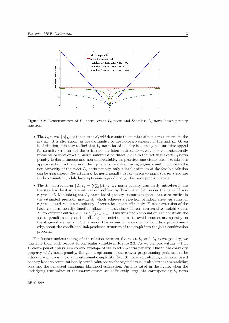
Figure 2.2: Demonstration of L1 norm, exact L0 norm and Seamless L0 norm based penaltyfunction.
• The L0 norm ‖A‖L0 of the matrix X, which counts the number of non-zero elements in thematrix. It is also known as the cardinality or the non-zero support of the matrix. Givenits definition, it is easy to find that L0 norm based penalty is a strong and intuitive appealfor sparsity structure of the estimated precision matrix. However, it is computationallyinfeasible to solve exact L0-norm minimization directly, due to the fact that exact L0 normpenalty is discontinuous and non-differentiable. In practice, one either uses a continuousapproximation to the form of the L0-penalty, or solve it using a greedy method. Due to thenon-convexity of the exact L0 norm penalty, only a local optimum of the feasible solutioncan be guaranteed. Nevertheless, L0 norm penalty usually leads to much sparser structurein the estimation, while local optimum is good enough for most practical cases.
• The L1 matrix norm ‖A‖L1 =∑ni,j |Aij |. L1 norm penalty was firstly introduced into
the standard least square estimation problem by Tibshiharni [34], under the name "Lassoregression”. Minimizing the L1 norm based penalty encourages sparse non-zero entries inthe estimated precision matrix A, which achieves a selection of informative variables forregression and reduces complexity of regression model efficiently. Further extension of thebasic L1-norm penalty function allows one assigning different non-negative weight valuesλij to different entries Aij , as
∑ni,j λij |Aij |. This weighted combination can constrain the
sparse penalties only on the off-diagonal entries, so as to avoid unnecessary sparsity onthe diagonal elements. Furthermore, this extension allows us to introduce prior knowl-edge about the conditional independence structure of the graph into the joint combinationproblem.
For further understanding of the relation between the exact L0 and L1 norm penalty, weillustrate them with respect to one scalar variable in Figure 2.2. As we can see, within [−1, 1],L1-norm penalty plays as a convex envelope of the exact L0-norm penalty. Due to the convexityproperty of L1 norm penalty, the global optimum of the convex programming problem can beachieved with even linear computational complexity [34, 13]. However, although L1 norm basedpenalty leads to computationally sound solutions to the original issue, it also introduces modelingbias into the penalized maximum likelihood estimation. As illustrated in the figure, when theunderlying true values of the matrix entries are sufficiently large, the corresponding L1 norm
RR n° 8059

14 Furtlehner & Han & others
based regularization performs linearly increased penalty to those entries, which thus results in asevere bias w.r.t. the maximum likelihood estimation [12]. In contrast, L0 norm based penaltyavoids such issue by constraining the penalties of non-zero elements to be constant. It has beenproved in [34] that the L1 norm penalty discovers the underlined sparse structure when somesuitable assumptions are satisfied. However, in general cases, the quality of the solutions is notclear.
3 Link selection at the Bethe point
3.1 Bethe approximation and Graph selection
As observed in the previous section, when using the Bethe approximation to find an approximatesolution to the IIP, the consistency check should then be that either the factor graph be sparse,nearly a tree, either the coupling are small. There are then two distinct ways of using the Betheapproximation:
• the direct way, where the form of the joint distribution (2.18) is assumed with a completegraph. There is then a belief propagation fixed point for which the beliefs satisfy all theconstraints. This solution to be meaningful requires small correlations, so that the beliefpropagation fixed point be stable and unique, allowing the corresponding log likelihood tobe well approximated. Otherwise, this solution is not satisfactory, but a pruning procedure,which amounts to select a sub-graph based on mutual information, can be used. The firststep is to find the MST with these weights. Adding new links to this baseline solution ina consistent way is the subject of the next section.
• the indirect way consists in first inverting the potentially non-sparse correlation matrix.If the underlying interaction matrix is actually a tree, this will be visible in the inversecorrelation matrix, indicated directly by the non-zero entries. This seems to work betterthan the previous one when no sparsity but weak coupling is assumed. It corresponds infact to the equations solved iteratively by the susceptibility propagation algorithm [28].
Let us first justify the intuitive assertion concerning the optimal model with tree like factorgraphs, which was actually first proposed in [6] and which is valid for any type of MRF.
Proposition 3.1. The optimal model with tree like factor graphs to the inverse pairwise MRFis obtained by finding the MST on the graph of weighted links with weights given by mutualinformation between variables.
Proof. On a tree, the Bethe distribution relating marginal pi of single and pair pij variablesdistributions
P(x) =∏
(i,j)∈T
pij(xi, xj)
pi(xi)pj(xj)
∏
i
pi(xi)
is exact. Assuming first that the associated factor graph is given by a tree T , the expression (2.6)of the log likelihood leads to the optimal solution given that tree:
pi = pi and pij = pij , ∀i ∈ V, (i, j) ∈ T .
In turn we have the following expression for the log likelihood:
L =∑
(i,j)∈T
Iij −∑
i
Hi,
Inria

Pairwise MRF Calibration 15
with
Hidef
= −∑
xi
pi(xi) log pi(xi)
Iijdef
=∑
xi,xj
pij(xi, xj) logpij(xi, xj)
pi(xi)pj(xj).
respectively the single variable entropy and the mutual information between two variables. Sincethe single variable contributions to the entropy is independent of the chosen graph T , the optimalchoice for T correspond to the statement of the proposition.
3.2 Optimal 1-link correction to the Bethe point
Adding one link Suppose now that we want to add one link to the max spanning tree.The question is which link will produce the maximum improvement to the log likelihood. Thisquestion is a special case of how to correct a given factor for a general pairwise model. Let P0
be the reference distribution to which we want to add (or modify) one factor ψij to produce thedistribution
P1(x) = P0(x) × ψij(xi, xj)
Zψ(3.1)
with
Zψ =
∫
dxidxjp0ij(xi, xj)ψij(xi, xj).
The log likelihood corresponding to this new distribution now reads
L1 = L0 +
∫
dxP(x) logψij(xi, xj) − logZψ.
The functional derivative w.r.t. ψ reads
∂L1
∂ψij(xi, xj)=
p(xi, xj)
ψij(xi, xj)−p0ij(xi, xj)
Zψ, ∀(xi, xj) ∈ Ω2.
which yield immediately the solution
ψij(xi, xj) =pij(xi, xj)
p0ij(xi, xj)
with Zψ = 1, (3.2)
where p0(xi, xj) is the reference marginal distribution obtained from P0. The correction to theLog likelihood simply reads
∆L = DKL(pij‖p0ij). (3.3)
Sorting all the links w.r.t. this quantity yields the (exact) optimal 1-link correction to be made.As a check, consider the special case of the Ising model. Adding one link amounts to set one
Jij to some finite value, but since this will perturb at least the local magnetization of i and j,we have also to modify the local fields hi and hj . The modified measure therefore reads
P1link = PBetheexp
(
Jijsisj + hisi + hjsj)
∆Z(J, h),
RR n° 8059

16 Furtlehner & Han & others
where ∆Z(J, h) is multiplicative correction factor to the partition function. We have
∆Z(hi, hj , Jij) = z0 + z1mi + z2mj + z3mBetheij ,
after introducing the following quantities
z0def
= eJij+hi+hj + e−Jij−hi+hj + e−Jij+hi−hj + eJij−hi−hj
z1def
= eJij+hi+hj − e−Jij−hi+hj + e−Jij+hi−hj − eJij−hi−hj
z2def
= eJij+hi+hj + e−Jij−hi+hj − e−Jij+hi−hj − eJij−hi−hj
z3def
= eJij+hi+hj − e−Jij−hi+hj − e−Jij+hi−hj + eJij−hi−hj .
The correction to the log likelihood is then given by
∆L(hi, hj , Jij) = log ∆Z(hi, hj , Jij) − himi − hjmj − Jijmij (3.4)
This is a concave function of hi, hj and Jij , and the (unique) maximum is obtained when thefollowing constraints are satisfied:
∂ log(∆Z)
∂hi=z1 + z0mi + z3mj + z2m
Betheij
∆Z(hi, hj , Jij)= mi,
∂ log(∆Z)
∂hj=z2 + z3mi + z0mj + z1m
Betheij
∆Z(hi, hj , Jij)= mj ,
∂ log(∆Z)
∂Jij=z3 + z2mi + z1mj + z0m
Betheij
∆Z(hi, hj , Jij)= mij .
This constraints can be solved as follows. First let
Udef
= (1 + mi + mj +mBetheij ) e2(hi+hj),
Vdef
= (1 − mi + mj −mBetheij ) e2(hj−Jij),
Wdef
= (1 + mi − mj −mBetheij ) e2(hi−Jij).
to obtain the linear system
U(1 − mi) − V (1 + mi) +W (1 − mi) = (1 − mi − mj +mBetheij )(1 + mi),
U(1 − mj) + V (1 − mj) −W (1 + mj) = (1 − mi − mj +mBetheij )(1 + mj),
U(1 − mij) − V (1 + mij) −W (1 + mij) = −(1 − mi − mj +mBetheij )(1 − mij).
Inverting this system yields the following solution
U =(1 − mi − mj +mBethe
ij )
(1 − mi − mj + mij)(1 + mi + mj + mij)
V =(1 − mi − mj +mBethe
ij )
(1 − mi − mj + mij)(1 − mi + mj − mij)
W =(1 − mi − mj +mBethe
ij )
(1 − mi − mj + mij)(1 + mi − mj − mij)
Inria

Pairwise MRF Calibration 17
Using the parametrization (2.20), we finally arrive at
ehisi+hjsj+Jijsisj =pij(si, sj)
bij(si, sj)
Åbij(1, 1)bij(−1, 1)bij(1,−1)bij(−1,−1)
pij(1, 1)pij(−1, 1)pij(1,−1)pij(−1,−1)
ã1/4
.
where bij(si, sj) is the joint marginal of si and sj , obtained from the Bethe reference point. Fromthese expressions, we can assess for any new potential link the increase (3.4) in the log likelihood.After rearranging all terms, it takes indeed as announced the following simple form
∆L(hi, hj , Jij) =∑
si,sj
pij logpij(si, sj)
bij(si, sj)= DKL(p‖b). (3.5)
The interpretation is therefore immediate: the best candidate is the one for which the Bethesolution yields the most distant joint marginal bij to the targeted one pij given by the data. Notethat the knowledge of the bij , (ij) /∈ T requires a sparse matrix inversion through equation(2.24), which renders the method a bit expensive in the Ising case. For Gaussian MRF, thesituation is different, because in that case the correction to the log likelihood can be evaluateddirectly by another means. Indeed, the correction factor (3.2) reads in that case
ψij(xi, xj) = exp(
−1
2(xi, xj)
(
[Cij ]−1 − [Cij ]−1)
(xi, xj)T)
,
where [Cij ] and [Cij ] represent the restricted 2 × 2 covariance matrix corresponding to the pair(xi, xj) of respectively the reference model and the current model specified by precision matrixA = C−1. With a small abuse of notation the new model obtained after adding or changing link(ij) reads
A′ = A+ [Cij ]−1 − [Cij ]−1 def
= A+ V.
with a log likelihoods variation given by:
∆L =CiiCjj + CjjCii − 2CijCij
CiiCjj − C2ij
− 2 − logCiiCjj − C2
ij
CiiCjj − C2ij
.
Let us notice the following useful formula (see e.g. [4]):
(A+ [V ij ])−1 = A−1 −A−1[V ij ](1 +A−1[V ij ])−1A−1
= A−1 −A−1[V ij ](1 + [Cij ][V ij ])−1A−1, (3.6)
valid for a 2× 2 perturbation matrix [V ij ]. Using this formula, the new covariance matrix reads
C ′ = A′−1 = A−1 −A−1[Cij ]−1(
1 − [Cij ][Cij ]−1)
A−1. (3.7)
Therefore the number of operations needed to maintain the covariance matrix after each add-onis O(N2).
Let us now examine under which condition adding/modifying links in this way let the co-variance matrix remain positive semi-definite. By adding a 2 × 2 matrix, we expect a quadratic
RR n° 8059

18 Furtlehner & Han & others
correction to the determinant:
det(A′) = det(A) det(1 +A−1V )
= det(A)[
1 + ViiCii + VijCji + VjiCij + VjjCjj
+(
ViiVjj − VijVji)(
CiiCjj − CijCji)
]
,
= detA× det([Cij ])
det([Cij ])
which is obtained directly because A−1V has non zero entries only on column i and j. MultiplyingV by some parameter α ≥ 0, define
P (α)def
= det(1 + αA−1V ) = α2 det(
[Cij ][Cij ]−1 − α− 1
α
)
.
When increasing α from 0 to 1, P (α) will vary from 1 to det([Cij ])/det([Cij ]) without cancelingat some point iff [Cij ][Cij ]−1 is definite positive. P (α) is proportional to the characteristicpolynomial of a 2×2 matrix [Cij ]/[Cij ]−1 of argument (α−1)/α, so A′ remains positive definiteif [Cij ][Cij ]−1 is definite positive. Since the product of eigenvalues given by det([Cij ])/det([Cij ])is positive, one has to check for the sum, given by the trace of [Cij ]/[Cij ]−1:
CiiCjj + CjjCii − 2CijCij > 0. (3.8)
Since [Cij ] and [Cij ] are individually positive definite, we have
CiiCjj − Cij2 > 0 and CiiCjj − C2
ij > 0
from which we deduce that
(CiiCjj + CjjCii2
)2
> CiiCjjCjjCii > Cij2C2
ij ,
giving finally that (3.8) is always fulfilled when both [Cij ] and [Cij ] are non-degenerate.Each time a link is added to the graph, its number of loops increases by one unit, so in a
sense (3.3) represent a 1-loop correction to the bare Bethe tree solution.
Removing one link To use this in an algorithm, it would also be desirable to be able toremove links as well, such that with help of a penalty coefficient per link, the model could beoptimized with a desired connectivity level.
For the Gaussian model, if A is the coupling matrix, removing the link (i, j) amounts to chosea factor ψij in (3.1) of the form:
ψij(xi, xj) = exp(
Aijxixj)
(xi and xj are assumed centered as in the preceding section). Again, let V denote the perturba-tion in the precision matrix such that A′ = A+ V is the new one. The corresponding change inthe log likelihood then reads
∆L = log det(1 +A−1V ) − Tr(V C).
Inria

Pairwise MRF Calibration 19
Arranging this expression leads to
∆L = log(
1 − 2AijCij −A2ij det([Cij ])
)
+ 2AijCij .
Using again (3.6) we get for the new covariance matrix
C ′ = C − Aij1 − 2AijCij −A2
ij det([Cij ])C
ñAijCjj 1 −AijCij
1 −AijCij AijCii
ôC, (3.9)
with again a slight abuse of notation, the 2 × 2 matrix being to be understood as a N × Nmatrix with non-zero entries corresponding to (i, i), (i, j), (j, i) and (j, j). To check for thepositive-definiteness property of A′, let us observe first that
det(A′) = det(A) × P (Aij),
withP (x) = (1 − x(Cij −
√
CiiCjj))(1 − x(Cij +√
CiiCjj)).
When x varies from 0 to Aij , P (x) should remains strictly positive to insure that A′ is definitepositive. This results in the following condition:
1
Cij −√
CiiCjj< Aij <
1√
CiiCjj + Cij.
We are now equipped to define algorithms based on addition/deletion of links.
3.3 Imposing walk-summability
Having a sparse GMRF gives no guaranty to its compatibility with belief propagation. In orderto be able to use the Gaussian Belief Propagation (GaBP) algorithm for performing inferencetasks, stricter constraints have to be imposed. The more precise condition known for convergenceand validity of the GaBP algorithm is called walk-summability (WS) and is extensively describedin [26]. The two necessary and sufficient conditions for WS that we consider here are:
(i) Diag(A) − |R(A)| is definite positive, with R(A)def
= A − Diag(A) the off-diagonal terms ofA.
(ii) The spectral radius ρ(|R′(A)|) < 1, with R′(A)ijdef
=R(A)ij√AiiAjj
.
Adding one link Using the criterion developed in the previous section suppose that in order toincrease the likelihood we wish to add a link (i, j) to the graph. The model is modified accordingto
A′ = A+ [Cij ]−1 − [Cij ]−1 def
= A+ V.
We assume that A is WS and we want to express conditions under which A′ is still WS.Using the definition (i) of walk summability and mimicking the reasoning leading to (3.8) we
can derive a sufficient condition for WS by replacing A with W (A)def
= Diag(A)−|R(A)|. It yields
det (W(A+ αV )) = det (W(A)) det(
1 + αW(A)−1W(V ))
= det (W )î1 + α
¶W−1ii Vii +W−1
jj Vjj − 2W−1ij |Vij |
©
+ α2ÄW−1ii W
−1jj − (W−1
ji )2ä
(
ViiVjj − |Vij |2)
ó
= det(W )Q(α),
RR n° 8059

20 Furtlehner & Han & others
since R(A)ij = 0 and shortening W (A) in W . A sufficient condition for WS of A′ is that Q doesnot have any root in [0, 1]. Note that checking this sufficient condition imposes to keep track of
the matrix (Diag(A) − |R|)−1 = W−1 def
= IW and requires O(N2) operations at each step, using(3.6). A more compact expression of Q is
Q(α) = 1 + αTr(
IW ijW (V ))
+ α2 det (W (V )) det(
IW ij)
,
First let’s tackle the special case where det(
W (V )IW ij)
= 0, the condition for WS of A′ is then
Tr(IW ijW (V )) > −1.
Of course if the roots are not real, i.e. Tr(IW ijW (V ))2 < 4 det(
W (V )IW ij)
, A′ is WS. If noneof these conditions is verified we have to check that both roots
−Tr(IW ijW (V ) ±√
Tr(IW ijW (V ))2 − 4 det (W (V )IW ij)
2 det (W (V )IW ij),
are not in [0, 1].
Modifying one link This is equivalent to adding one link in the sense that (3.1) and (3.2)are still valid. If we want to make use of (i) the only difference is that R(A)ij is not zero beforeadding V so W (A+ αV ) = W (A) + αW (V ) does not hold in general. Instead we have
W (A+ αV ) = W (A) + φ(αV,A),
with
φ(V,A)def
=
ïVii −|Vij +Aij | + |Aij |
−|Vji −Aji| + |Aij | Vjj
ò
So we can derive a condition for A′ to be WS using, as for the link addition,
det(W (A+ αV )) = det (W ) det(
1 +W−1φ(αV,A))
= det (W ) Θ(α)
But now Θ(α), the equivalent of Q(α), is a degree 2 polynomial only by parts. More precisely, if
αVij − Aij > 0 we have Θ(α)def
= Qp(α) and else Θ(α)def
= Qm(α) with both Qp and Qm degree 2polynomial. So by checking the sign of αVij −Aij and the roots of Qp and Qm we have sufficientconditions for WS after modifying one link.
Another possible way for both adding or modifying one link is to estimate the spectral radiusof |R′(A′)| through simple power iterations and concludes using (ii). Indeed if a matrix M as aunique eigenvalue of modulus equal to its spectral radius then the sequence
µkdef
=〈bk,Mbk〉〈bk, bk〉
, with bk+1def
=Mbk
‖Mbk‖
converges to this eigenvalue. While the model remains sparse, with connectivity K, a poweriteration of R′(A′) requires O(KN) operations, and it is then possible to conclude about the WSof A′ in O(KN). Keeping track of W (A)−1, which requires O(N2) operations, at each step is notneeded anymore but we have to test WS for each possible candidate link. Note that computingthe spectral radius gives us a more precise information about the WS status of the model.
Inria

Pairwise MRF Calibration 21
Removing one link Removing one link of the graph will change the matrix A in A′ suchas |R′(A′)| ≤ |R′(A)| where the comparison (≤) between two matrices must be understood asthe element-wise comparison. Then dealing with positive matrices elementary results gives usρ(|R′(A′)|) ≤ ρ(|R′(A)|) and thus removing one link of a WS model provide a new WS model.
3.4 Greedy Graph construction Algorithms
Algorithm 1: Incremental graph construction by link addition
S1 INPUT: the MST graph, and corresponding covariance matrix C.
S2 : select the link with highest ∆L compatible with the WS preserving condition of A′ in theGaussian case. Update C according to (3.7) for the Gaussian model. For the Ising model,C is updated by first running BP to generate the set of beliefs and co-beliefs supportedby the current factor graph, which in turn allows one to use (2.24) to get all the missingentries in C by inverting χ−1.
S3 : repeat S2 until convergence (i) or until a target connectivity is reached (ii)
S4 : if (ii) repeat S2 until convergence by restricting the link selection in the set of existingones.
The complexity is respectively O(N3) both for the Gaussian and the Ising model in the sparsedomain where O(N) links are added and respectively O(N4) and O(N5) in the dense domain.Indeed, the inversion of χ−1 in the Ising case costs O(N2) operations as long as the factor graphremains sparse, but O(N3) for dense matrices.
Algorithm 2: Graph surgery by link addition/deletion
S1 INPUT: the MST graph, and corresponding covariance matrix C, a link penalty coefficientν.
S2 : select the modification with highest ∆L−sν, with s = +1 for an addition and s = −1 for adeletion, compatible with the WS preserving condition of A′ in the Gaussian case. UpdateC according to (3.7) and (3.9) respectively for an addition or a change and a deletion forthe Gaussian model. For the Ising model, C is updated by first running BP to generatethe set of beliefs and co-beliefs supported by the current factor graph, which in turn allowsone to use (2.24) to get all the missing entries in C by inverting χ−1.
S3 : repeat S2 until convergence.
In absence of penalty (ν = 0) the algorithm will simply generate a model for all different meanconnectivities, hence delivering an almost continuous Pareto set of solutions, with all possibletrade-off between sparsity and likelihood as long as walk summability is satisfied.
Instead, with a fixed penalty the algorithm is converging toward a solution with a connectivitydepending implicitly on ν; it corresponding roughly to the point K⋆ where the slope is
∆LN∆K
(K⋆) = ν.
If we want to use the backtracking mechanism allowed by the penalty term without convergingto a specific connectivity, we may also let ν be adapted dynamically. A simple way is to adaptν with the rate of information gain by letting
ν = η∆Ladd, with η ∈ [0, 1[,
RR n° 8059

22 Furtlehner & Han & others
where ∆Ladd corresponds to the gain of the last link addition. With such a setting ν is alwaysmaintained just below the information gain per link, allowing thus the algorithm to carry ontoward higher connectivity. Of course this heuristic assumes a concave Pareto front.
4 Perturbation theory near the Bethe point
4.1 Linear response of the Bethe reference point
The approximate Boltzmann machines described in the introduction are obtained either by per-turbation around the trivial point corresponding to a model of independent variables, the firstorder yielding the Mean-field solution and the second order the TAP one, either by using thelinear response delivered in the Bethe approximation. We propose to combine in a way the twoprocedures, by computing the perturbation around the Bethe model associated to the MST withweights given by mutual information. We denote by T ⊂ E , the subset of links correspondingto the MST, considered as given as well as the susceptibility matrix [χBethe] given explicitly byits inverse through (2.24), in term of the empirically observed ones χ. Following the same linesas the one given in Section 2, we consider again the Gibbs free energy to impose the individualexpectations m = mi given for each variable. Let J
Bethe = Kij , (i, j) ∈ T the set of Bethe-Ising couplings, i.e. the set of coupling attached to the MST s.t. corresponding susceptibilitiesare fulfilled and J = Jij , (i, j) ∈ E a set of Ising coupling corrections. The Gibbs free energyreads now
G[m,J] = hT (m)m + F
[
h(m),JBethe + J]
where h(m) depends implicitly on m through the same set of constraints (2.7) as before. Theonly difference resides in the choice of the reference point. We start from the Bethe solutiongiven by the set of coupling J
Bethe instead of starting with an independent model.
The Plefka expansion is used again to expand the Gibbs free energy in power of the couplingJij assumed to be small. Following the same lines as in Section 2.1, but with G0 now replacedby
GBethe[m] = hT (m)m − logZBethe
[
h(m),JBethe]
,
and hi, JBethe and ZBethe given respectively by (2.21,2.22,2.23) where E is now replaced by T ,
letting again
H1 def
=∑
i<j
Jijsisj ,
and following the same steps (2.13,2.14,2.15) leads to the following modification of the local fields
hi = hBethei −∑
j
[χ−1Bethe]ij CovBethe(H
1, si) ∀i ∈ V
to get the following Gibbs free energy at second order in α (after replacing H1 by αH1):
G[m, αJ ] = GBethe(m) − αEBethe(H1)
−α2
2
(
VarBethe(H1) −
∑
ij
[χ−1Bethe]ij CovBethe(H
1, si) CovBethe(H1, sj)
)
+ o(α2).
Inria
Pairwise MRF Calibration 23
This is the general expression for the linear response near the Bethe reference point that we nowuse.
GBLR[J]def
= −EBethe(H1) (4.1)
− 1
2
(
VarBethe(H1) −
∑
i,j
[χ−1Bethe]ij CovBethe(H
1, si) CovBethe(H1, sj)
)
. (4.2)
represents the Gibbs free energy at this order of approximation. It it is given explicitly through
EBethe(H1) =
∑
i<j
Jijmij
VarBethe(H1) =
∑
i<j,k<l
JijJkl(
mijkl −mijmkl
)
CovBethe(H1, sk) =
∑
i<j
Jij(mijk −mijmk)
where
midef
= EBethe(si), mijdef
= EBethe(sisj)
mijkdef
= EBethe(sisjsk), mijkldef
= EBethe(sisjsksl)
are the moments delivered by the Bethe approximation. With the material given in Section 2.2these are given in closed form in terms of the Bethe susceptibility coefficients χBethe. Concerningthe log-likelihood, it is given now by:
L[J] = −GBethe(m) −GBLR[J] −∑
ij
(JBetheij + Jij)mij + o(J2). (4.3)
GBLR is at most quadratic in the J ’s and contains the local projected Hessian of the log likelihoodonto the magnetization constraints (2.7) with respect to this set of parameters. This is nothingelse than the Fisher information matrix associated to these parameter J which is known to bepositive-semidefinite, which means that the log-likelihood associated to this parameter space isconvex. Therefore it makes sense to use the quadratic approximation (4.3) to find the optimalpoint.
4.2 Line search along the natural gradient in a reduced space
Finding the corresponding couplings still amounts to solve a linear problem of size N2 in thenumber of variables which will hardly scale up for large system sizes. We have to resort to somesimplifications which amounts to reduce the size of the problem, i.e. the number of independentcouplings. To reduce the problem size we can take a reduced number of link into consideration,i.e. the one associated with a large mutual information or to partition them in a way whichremains to decide, into a small number q of group Gν , ν = 1, . . . q. Then, to each group ν isassociated a parameter αν with a global perturbation of the form
H1 =
q∑
ν=1
ανHν
RR n° 8059

24 Furtlehner & Han & others
where each Hν involves the link only present in Gν .
Hνdef
=∑
(i,j)∈Gν
Jijsisj ,
and the Jij are fixed in some way to be discussed soon. The corresponding constraints, whichultimately insures a max log-likelihood in this reduced parameter space are then
∂GBLR∂αν
= −E(Hν).
This leads to the solution:
αµ =
q∑
ν=1
I−1µν
(
E(Hν) − EBethe(Hν))
where the Fisher information matrix I has been introduced and which reads in the present case
Iµν =[
CovBethe(Hµ, Hν) −∑
i6=j(i,j)∈T
[χ−1Bethe]ij CovBethe(Hµ, si) CovBethe(Hν , sj)
]
(4.4)
The interpretation of this solution is to look in the direction of the natural gradient [1, 3] ofthe log likelihood. The exact computation of the entries of the Fisher matrix involves up to4th order moments and can be computed using results of Section 2.2. At this point, the wayof choosing the groups of edges and the perturbation couplings Jij of the corresponding links,leads to various possible algorithms. For example, to connect this approach to the one proposedin Section 3.2, the first group of links can be given by the MST, with parameter α0 and theiractual couplings Jij = JBetheij at the Bethe approximation; making a short list of the q − 1 bestlinks candidates to be added to the graph, according to the information criteria 3.3, defines theother groups as singletons. It is then reasonable to attach them the value
Jij =1
4log
p11ij
p11ij
p00ij
p00ij
p01ij
p01ij
p10ij
p10ij
,
of the coupling according to (3.2), while the modification of the local fields as a consequence of(3.2) can be dropped since the Gibbs free energy take it already into account implicitly, in orderto maintain single variable magnetization mi = mi correctly imposed.
4.3 Reference point at low temperature
Up to now we have considered the case where the reference model is supposed to be a treeand is represented by a single BP fixed point. From the point of view of the Ising model thiscorresponds to perturb a high temperature model in the paramagnetic phase. In practice thedata encountered in applications are more likely to be generated by a multi-modal distributionand a low temperature model with many fixed points should be more relevant. In such a casewe assume that most of the correlations are already captured by the definition of single beliefsfixed points and the residual correlations is contained in the co-beliefs of each fixed point. For amulti-modal distribution with q modes with weight wk, k = 1 . . . q and a pair of variables (si, sj)we indeed have
χij =
q∑
k=1
wk Cov(si, sj |k) +
q∑
k=1
wk(E(si|k) − E(si))(E(sj |k) − E(sj))
def
= χintraij + χinterij ,
Inria
Pairwise MRF Calibration 25
where the first term is the average intra cluster susceptibility while the second is the inter clustersusceptibility. All the preceding approach can then be followed by replacing the single Bethesusceptibility and higher order moments in equations (4.1,4.4) in the proper way by their multipleBP fixed point counterparts. For the susceptibility coefficients, the inter cluster susceptibilitycoefficients χinter are given directly from the single variable belief fixed points. The intra clustersusceptibilities χk are treated the same way as the former Bethe susceptibility. This means thatthe co-beliefs of fixed points k ∈ 1, . . . q are entered in formula (2.24) which by inversion yieldsthe χk’s, these in turn leading to χintra by superposition. Higher order moments are obtain bysimple superposition. Improved models could be then searched along the direction indicated bythis natural gradient.
5 L0 norm penalized sparse inverse estimation algorithm
We propose here to use the Doubly Augmented Lagrange (DAL) method [22, 11, 10] to solve thepenalized log-determinant programming in (2.28). For a general problem defined as follows:
minxF (x) = f(x) + g(x) (5.1)
where f(x) and g(x) are both convex. DAL splits the combination of f(x) and g(x) by introducinga new auxiliary variable y. Thus, the original convex programming problem can be formulatedas :
minx,y
F (x) = f(x) + g(y)
s.t. x− y = 0(5.2)
Then it advocates an augmented Lagrangian method to the extended cost function in (5.2).Given penalty parameters µ and γ, it minimizes the augmented Lagrangian function
L(x, y, ν, x, y) = f(x) + g(y) + 〈ν, x− y〉 +µ
2‖x− y‖2
2 +γ
2‖x− x‖2
2 +γ
2‖y − y‖2
2 (5.3)
where x and y are the prior guesses of x and y that can obtained either from a proper initializationor the estimated result in the last round of iteration in an iterative update procedure. Sinceoptimizing jointly with respect to x and y is usually difficult, DAL optimizes x and y alternatively.That gives the following iterative alternative update algorithm with some simple manipulations:
xk+1 = minxf(x) +
µ
2‖x− yk + νk‖2
2 +γ
2‖x− xk‖2
2
yk+1 = minyg(y) +
µ
2‖xk+1 − y + νk‖2
2 +γ
2‖y − yk‖2
2
νk+1 = νk + xk+1 − yk+1
(5.4)
where ν = 1µν. As denoted in [10] and [22], DAL improves basic augmented Lagrangian opti-
mization by performing additional smooth regularization on estimations of x and y in successiveiteration steps. As a result, it guarantees not only the convergence of the scaled dual variable ν,but also that of the proximal variables xk and yk, which could be divergent in basic augmentedLagrangian method.
We return now to the penalized log-determinant programming in sparse inverse estimationproblem, as seen in (2.28). The challenge of optimizing the cost function is twofold. Firstly,the exact L0-norm penalty is non-differentiable, making it difficult to find an analytic form ofgradient for optimization. Furthermore, due to the log-determinant term in the cost function,it implicitly requires that any feasible solution to the sparse approximation A of the precision
RR n° 8059
26 Furtlehner & Han & others
matrix should be strictly positive definite. The gradient of the log-determinant term is givenby C −A−1, which is not continuous in the positive definite domain and makes it impossible toobtain any second-order derivative information to speed up the gradient descent procedure. Wehereafter use S++ as the symmetric positive definite symmetric matrices that form the feasiblesolution set for this problem. By applying DAL to the cost function (2.28), we can derive thefollowing formulation:
J(A,Z, A, Z, ν) = − log det(A) + Tr(CA) + λP (Z) + 〈ν,A− Z〉+µ
2‖A− Z‖2
2 +γ
2‖A− A‖2
2 +γ
2‖Z − Z‖2
2
s.t. A,Z ∈ S++
(5.5)
where Z is the auxiliary variable that has the same dimension as the sparse inverse estimationA. A and Z are the estimated values of A and Z derived in the last iteration step. The penaltyparameter γ controls the regularity of A and Z. By optimizing A and Z alternatively, the DALprocedure can be easily formulated as an iterative process as follows, for some δ > 0:
Ak+1 = argminA
− log det(A) + Tr(CA) + λP (Zk) + 〈νk, A− Zk〉
+µ
2‖A− Zk‖2
2 +γ
2‖A−Ak‖2
2
Zk+1 = argminZ
λP (Z) + 〈νk, Ak+1 − Z〉 +µ
2‖Ak+1 − Z‖2
2
+γ
2‖Z − Zk‖2
2
νk+1 = νk + δ(Ak+1 − Zk+1)
s.t. Ak+1, Zk+1 ∈ S++
(5.6)
By introducing the auxiliary variable Z, the original penalized maximum likelihood problemis decomposed into two parts. The first one is composed mainly by the convex log-determinantprogramming term. Non-convex penalty is absorbed into the left part. Separating the likelihoodfunction and the penalty leads to the simpler sub-problems of solving log-determinant program-ming using eigenvalue decomposition and L0 norm penalized sparse learning alternatively. Eachsub-problem contains only one single variable, making it applicable to call gradient descent op-eration to search local optimum. Taking ν = 1
µν, we can derive the following scaled version ofDAL for the penalized log-determinant programming:
Ak+1 = argminA
− log det(A) + Tr(CA) +µ
2
∥
∥A− Zk + νk∥
∥
2
2+γ
2
∥
∥A−Ak∥
∥
2
2
Zk+1 = argminZ
µ
2
∥
∥Ak+1 − Z + νk∥
∥
2
2+γ
2
∥
∥Z − Zk∥
∥
2
2+ λP (Z)
νk+1 = νk +Ak+1 − Zk+1
s.t. Ak+1, Zk+1 ∈ S++
(5.7)
To attack the challenge caused by non-differentiability of the exact L0 norm penalty, wemake use of a differentiable approximation to L0-norm penalty in the cost function J , named as"seamless L0 penalty” (SELO) in [25]. The basic definition of this penalty term is given as:
PSELO(Z) =∑
i,j
1
log(2)log(1 +
|Zi,j ||Zi,j | + τ
) (5.8)
Inria
Pairwise MRF Calibration 27
where Zi,j denotes individual entry in the matrix Z and τ > 0 is a tuning parameter. As seenin Figure 2.2, as τ gets smaller, P (Zi,j) approximates better the L0 norm I(Zi,j 6= 0). SELOpenalty is differentiable, thus we can calculate the gradient of P (Z) explicitly with respect toeach Zi,j and make use of first-order optimality condition to search local optimum solution. Dueto its continuous property, it is more stable than the exact L0 norm penalty in optimization. Asproved in [25], the SELO penalty has the oracle property with proper setting of τ . That’s to say,the SELO penalty is asymptotically normal with the same asymptotic variance as the unbiasedOLS estimator in terms of Least Square Estimation problem.
The first two steps in (5.7) are performed with the positive definite constrains imposed on Aand Z. The minimizing with respect to A is accomplished easily by performing Singular VectorDecomposition (SVD). By calculating the gradient of J with respect to A in (5.7), based on thefirst-order optimality, we derive:
C −A−1 + µ(A− Zk + νk) + γ(A−Ak) = 0 (5.9)
Based on generalized eigenvalue decomposition, it is easy to verify that Ak+1 = V Diag(β)V T ,where V and di are the eigenvectors and eigenvalues of µ(Zk − νk) − C + γAk. βi is definedas:
βi =di +»di
2 + 4(ν + γ)
2(ν + γ)(5.10)
Imposing Z ∈ S++ directly in minimizing the cost function with respect to Y make the opti-mization difficult to solve. Thus, instead, we can derive a feasible solution to Z by a continuoussearch on µ. Based on spectral decomposition, it is clear that Xk+1 is guaranteed to be positivedefinite, while it is not necessarily sparse. In contrast, Z is regularized to be sparse while notguaranteed to be positive definite. µ is the regularization parameter controlling the margin be-tween the estimated Xk+1 and the sparse Zk+1. Increasingly larger µ during iterations makesthe sequences Xk and Zk converge to the same point gradually by reducing margin betweenthem. Thus, with enough iteration steps, the derived Zk follows the positive definite constraintand sparsity constraint at the same time. We choose here to increase µ geometrically with apositive factor η > 1 after every Nµ iterations until its value achieves a predefined upper boundµmax. With this idea, the iterative DAL solution to the L0 norm penalty is given as:
Ak+1 = argminA
− log det(A) + Tr(CA) +µ
2
∥
∥A− Zk + νk∥
∥
2
2+γ
2
∥
∥A−Ak∥
∥
2
2,
Zk+1 = argminZ
µ
2
∥
∥Ak+1 − Z + νk∥
∥
2
2+γ
2
∥
∥Z − Zk∥
∥
2
2+ λP (Z)
νk+1 = νk +Ak+1 − Zk+1
µk+1 = min(
µ η⌊k/Nµ⌋, µmax
)
.
(5.11)
In the second step of (5.11), we calculate the gradient of the cost function with respect to Zand achieve the local minimum by performing the first-order optimum condition on it. Therefore,the updated value of each entry of Z is given by a root of a cubic equation, as defined below:
if Zi,j > 0, Zi,j is the positive root of
2Zi,j3 + (3τ − 2θi,j)Zi,j
2 + (τ2 − 3τθi,j)Zi,j − τ2θi,j +λτ
µ+ γ= 0
if Zi,j < 0, Zi,j is the negative root of
2Zi,j3 − (3τ + 2θi,j)Zi,j
2 + (τ2 + 3τθi,j)Zi,j − τ2θi,j −λτ
µ+ γ= 0
else Zi,j = 0
(5.12)
RR n° 8059

28 Furtlehner & Han & others
where Zi,j is one single entry of Z and
θi,j =γZki,j + µ(Ak+1
i,j + νk)
µ+ γ.
Solving the cubic equations can be done rapidly using Cardano’s formula within a time costO(n2). Besides, the spectral decomposition procedure has the general time cost O(n3). Giventhe total number of iterations K, theoretical computation complexity of DAL is O(Kn3). Forour experiments, we initialize µ to 0.06, the multiplier factor η to 1.3 and the regularizationpenalty parameter γ to 10−4. To approximate the L0 norm penalty, τ is set to be 5 ·10−4. In ourexperiment, to derive the Pareto curve of the optimization result, we traverse different values ofλ. Most learning procedures converge with no more than K = 500 iteration steps.
To validate performance of sparse inverse estimation based on the L0 norm penalty, we involvean alternative sparse inverse matrix learning method using L1 norm penalization for comparison.Taking P (A) in (2.28) to be the L1 matrix norm of A, we strengthen conditional dependencestructure between random variables by jointly minimizing the negative log likelihood functionand the L1 norm penalty of the inverse matrix. Since L1 norm penalty is strictly convex, wecan use a quadratic approximation to the cost function to search for the global optimum, whichavoids singular vector decomposition with complexity of O(p3) and improves the computationalefficiency of this solution to O(p), where p is the number of random variables in the GMRFmodel. This quadratic approximation based sparse inverse matrix learning is given in [5], namedas QUIC. We perform it directly on the empirical covariance matrix with different settings ofthe regularization coefficient λ. According to works in compressed sensing, the equality betweenL1 norm penalty and L0 norm penalty holds if and only if the design matrix satisfies restrictedisometry property. However, restricted isometry property is sometimes too strong in practicalcase. Furthermore, to our best knowledge, there is no similar necessary condition guaranteeingequivalence between L1 and L0 norm penalty in sparse inverse estimation problem. Therefore,in our case, L1 norm penalized log-determinant programming is highly likely to be biased fromthe underlying sparse correlation structure in the graph, which leads to much denser inversematrices.
6 Experiments
In this section, various solutions based on the different methods exposed before are compared.We look first at the intrinsic quality, given either by the exact log likelihood for the Gaussian case,or by the empirical one for the Ising model, and then at its compatibility with belief propagationfor inference tasks.
Inverse Ising problem Let us start with the inverse Ising problem. The first set of ex-periments illustrates how the linear-response approach exposed in Section 2 works when theunderlying model to be found is itself an Ising model. The quality of the solution can thenbe assessed directly by comparing the couplings Jij found with the actual ones. Figure 6.1 areobtained by generating at random 103 Ising models of small size N = 10 either with no localfields (hi = 0,∀i = 1 . . . N) or with random centered ones hi = U [0, 1] − 1/2 and with couplingsJij = J√
N/3(2 ∗ U [0, 1] − 1), centered with variance J2/N , J being the common rescaling factor
corresponding to the inverse temperature. A glassy transition is expected at J = 1. The cou-plings are then determined using (2.16), (2.17), (2.22) and (2.25) respectively for the mean-field,TAP, BP and Bethe (equivalent to susceptibility propagation) solutions. Figure 6.1.a shows that
Inria
Pairwise MRF Calibration 29
0,0001 0,001 0,01 0,1 1
J
1e-15
1e-14
1e-13
1e-12
1e-11
1e-10
1e-09
1e-08
1e-07
1e-06
1e-05
0,0001
0,001
0,01
0,1
RM
SE(J
ij/J) MF
TAPBetheBP
<Jij>=0 hi=0
0,0001 0,001 0,01 0,1 1
J
1e-10
1e-09
1e-08
1e-07
1e-06
1e-05
0,0001
0,001
0,01
0,1
1
RM
SE(J
ij/J)
MFTAPBetheBP
<Jij>=0 <hi>=0
(a) (b)
0,0001 0,001 0,01 0,1 1
J
1e-14
1e-12
1e-10
1e-08
1e-06
0,0001
0,01
1
100
10000
1e+06
1e+08
RM
SE(X
ij/J)
MFTAPBetheBP
<Jij>=0 hi=0
0,0001 0,001 0,01 0,1 1
J
1e-10
1e-08
1e-06
0,0001
0,01
1
100
10000
1e+06
1e+08
RM
SE(X
ij/J)
MFTAPBetheBP
<Jij>=0 <hi>=0
(c) (d)
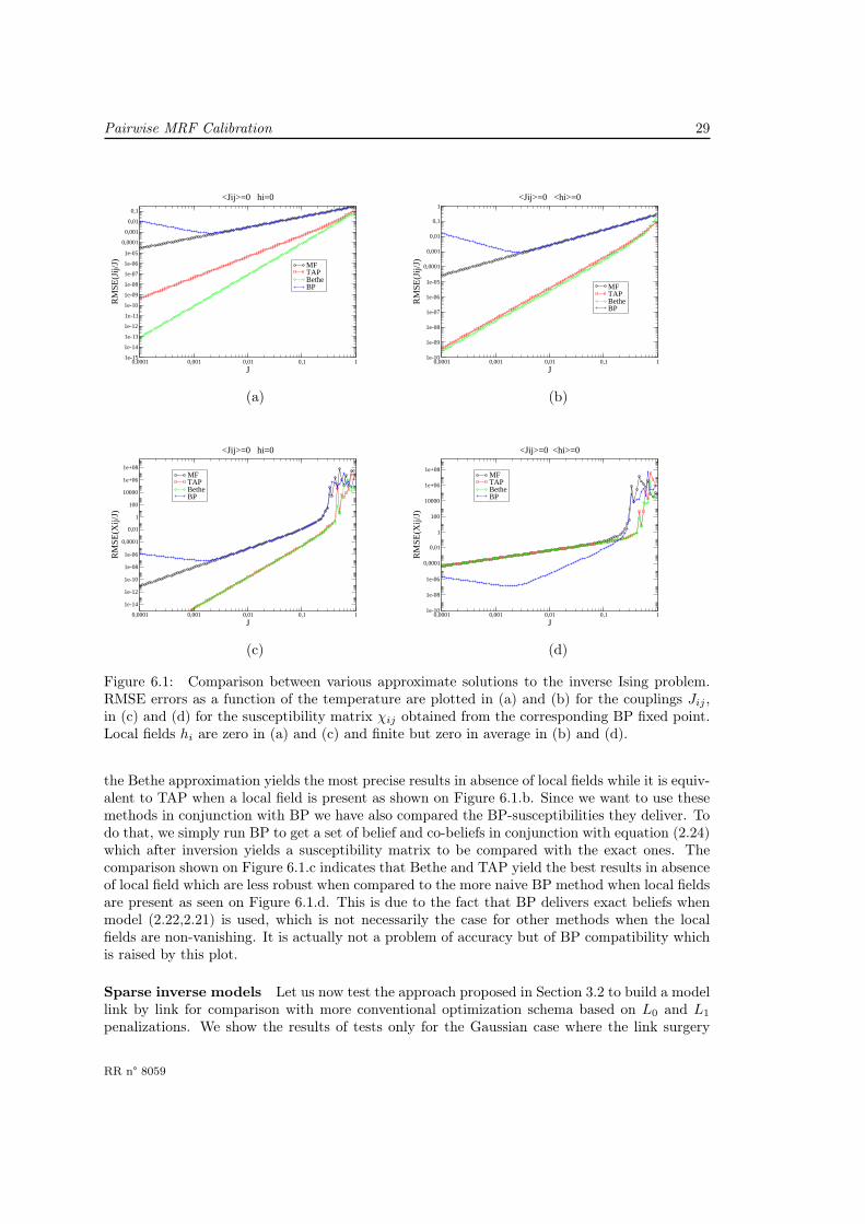
Figure 6.1: Comparison between various approximate solutions to the inverse Ising problem.RMSE errors as a function of the temperature are plotted in (a) and (b) for the couplings Jij ,in (c) and (d) for the susceptibility matrix χij obtained from the corresponding BP fixed point.Local fields hi are zero in (a) and (c) and finite but zero in average in (b) and (d).
the Bethe approximation yields the most precise results in absence of local fields while it is equiv-alent to TAP when a local field is present as shown on Figure 6.1.b. Since we want to use thesemethods in conjunction with BP we have also compared the BP-susceptibilities they deliver. Todo that, we simply run BP to get a set of belief and co-beliefs in conjunction with equation (2.24)which after inversion yields a susceptibility matrix to be compared with the exact ones. Thecomparison shown on Figure 6.1.c indicates that Bethe and TAP yield the best results in absenceof local field which are less robust when compared to the more naive BP method when local fieldsare present as seen on Figure 6.1.d. This is due to the fact that BP delivers exact beliefs whenmodel (2.22,2.21) is used, which is not necessarily the case for other methods when the localfields are non-vanishing. It is actually not a problem of accuracy but of BP compatibility whichis raised by this plot.
Sparse inverse models Let us now test the approach proposed in Section 3.2 to build a modellink by link for comparison with more conventional optimization schema based on L0 and L1
penalizations. We show the results of tests only for the Gaussian case where the link surgery
RR n° 8059
30 Furtlehner & Han & others
1 10 100<K>
-20
-10
0
10
20
LL
GreedyL0L1Reference
Sioux-Falls
1 10 100 1000<K>
0
500
1000
1500
2000
LL
L0L1GreedyReference
IAU
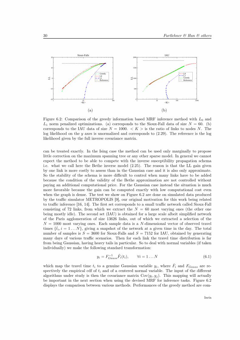
(a) (b)
Figure 6.2: Comparison of the greedy information based MRF inference method with L0 andL1 norm penalized optimizations. (a) corresponds to the Sioux-Fall data of size N = 60. (b)corresponds to the IAU data of size N = 1000. < K > is the ratio of links to nodes N . Thelog likelihood on the y axes is unormalized and corresponds to (2.29). The reference is the loglikelihood given by the full inverse covariance matrix.
can be treated exactly. In the Ising case the method can be used only marginally to proposelittle correction on the maximum spanning tree or any other sparse model. In general we cannotexpect the method to be able to compete with the inverse susceptibility propagation schemai.e. what we call here the Bethe inverse model (2.25). The reason is that the LL gain givenby one link is more costly to assess than in the Gaussian case and it is also only approximate.So the stability of the schema is more difficult to control when many links have to be addedbecause the condition of the validity of the Bethe approximation are not controlled withoutpaying an additional computational price. For the Gaussian case instead the situation is muchmore favorable because the gain can be computed exactly with low computational cost evenwhen the graph is dense. The test we show on Figure 6.2 are done on simulated data producedby the traffic simulator METROPOLIS [9], our original motivation for this work being relatedto traffic inference [16, 14]. The first set corresponds to a small traffic network called Sioux-Fallconsisting of 72 links, from which we extract the N = 60 most varying ones (the other onebeing mostly idle). The second set (IAU) is obtained for a large scale albeit simplified networkof the Paris agglomeration of size 13626 links, out of which we extracted a selection of theN = 1000 most varying ones. Each sample data is a N -dimensional vector of observed traveltimes ti, i = 1 . . . N, giving a snapshot of the network at a given time in the day. The totalnumber of samples is S = 3600 for Sioux-Falls and S = 7152 for IAU, obtained by generatingmany days of various traffic scenarios. Then for each link the travel time distribution is farfrom being Gaussian, having heavy tails in particular. So to deal with normal variables (if takenindividually) we make the following standard transformation:
yi = F−1GaussFi(ti), ∀i = 1 . . . N (6.1)
which map the travel time ti to a genuine Gaussian variable yi, where Fi and FGauss are re-spectively the empirical cdf of ti and of a centered normal variable. The input of the differentalgorithms under study is then the covariance matrix Cov(yi, yj). This mapping will actuallybe important in the next section when using the devised MRF for inference tasks. Figure 6.2displays the comparison between various methods. Performances of the greedy method are com-
Inria
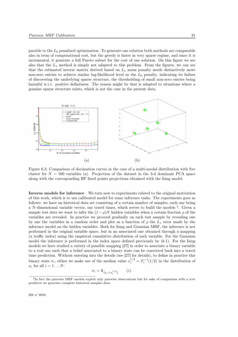
Pairwise MRF Calibration 31
parable to the L0 penalized optimization. To generate one solution both methods are comparablealso in term of computational cost, but the greedy is faster in very sparse regime, and since it isincremental, it generate a full Pareto subset for the cost of one solution. On this figure we seealso that the L1 method is simply not adapted to this problem. From the figures, we can seethat the estimated inverse matrix derived based on L1 norm penalty needs distinctively morenon-zero entries to achieve similar log-likelihood level as the L0 penalty, indicating its failureof discovering the underlying sparse structure, the thresholding of small non-zero entries beingharmful w.r.t. positive definitness. The reason might be that is adapted to situations where agenuine sparse structure exists, which is not the case in the present data.
0 0,2 0,4 0,6 0,8 1
% of revealed variables
0,5
0,6
0,7
0,8
0,9
1
L1
ER
RO
R
GaBP <K>=20BP alpha=0.04 <K> = 71KNNExact GaussianGround truth
N=500 C=5
(a) (b)
Figure 6.3: Comparison of decimation curves in the case of a multi-modal distribution with fivecluster for N = 500 variables (a). Projection of the dataset in the 3-d dominant PCA spacealong with the corresponding BP fixed points projections obtained with the Ising model.
Inverse models for inference We turn now to experiments related to the original motivationof this work, which is to use calibrated model for some inference tasks. The experiments goes asfollows: we have an historical data set consisting of a certain number of samples, each one beinga N -dimensional variable vector, say travel times, which serves to build the models 2. Given asample test data we want to infer the (1− ρ)N hidden variables when a certain fraction ρ of thevariables are revealed. In practice we proceed gradually on each test sample by revealing oneby one the variables in a random order and plot as a function of ρ the L1 error made by theinference model on the hidden variables. Both for Ising and Gaussian MRF, the inference is notperformed in the original variable space, but in an associated one obtained through a mapping(a traffic index) using the empirical cumulative distribution of each variable. For the Gaussianmodel the inference is performed in the index space defined previously by (6.1). For the Isingmodels we have studied a variety of possible mapping [27] in order to associate a binary variableto a real one such that a belief associated to a binary state can be converted back into a traveltime prediction. Without entering into the details (see [27] for details), to define in practice this
binary state σi, either we make use of the median value x1/2i = F−1
i (1/2) in the distribution ofxi for all i = 1 . . . N :
σi = 11xi>x
1/2i
(i).
2In fact the pairwise MRF models exploit only pairwise observations but for sake of comparison with a knn
predictor we generate complete historical samples data.
RR n° 8059
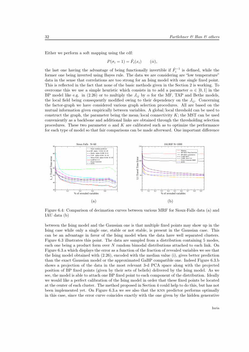
32 Furtlehner & Han & others
Either we perform a soft mapping using the cdf:
P (σi = 1) = Fi(xi) (ii),
the last one having the advantage of being functionally invertible if F−1i is defined, while the
former one being inverted using Bayes rule. The data we are considering are “low temperature”data in the sense that correlations are too strong for an Ising model with one single fixed point.This is reflected in the fact that none of the basic methods given in the Section 2 is working. Toovercome this we use a simple heuristic which consists in to add a parameter α ∈ [0, 1] in theBP model like e.g. in (2.26) or to multiply the Jij by α for the MF, TAP and Bethe models,the local field being consequently modified owing to their dependency on the Jij . Concerningthe factor-graph we have considered various graph selection procedures. All are based on themutual information given empirically between variables. A global/local threshold can be used toconstruct the graph, the parameter being the mean/local connectivity K; the MST can be usedconveniently as a backbone and additional links are obtained through the thresholding selectionprocedures. These two parameter α and K are calibrated such as to optimize the performancefor each type of model so that fair comparisons can be made afterward. One important difference
0 0,2 0,4 0,6 0,8 1
% of revealed variables
30
40
50
60
70
80
90
L_1
Tra
vel T
ime
erro
r
Static median predictorBP alpha = 0.024 K=28Bethe alpha=0.098 K=8TAP alpha=0.041 K=16Mean Field alpha=0.044 K=20GaBP K=2.5Exact GaussianKNN
Sioux Falls N=60
0 0,1 0,2 0,3 0,4 0,5 0,6 0,7 0,8 0,9
% of revealed variables
0
50
100
150
L1
Tra
vel T
ime
Err
or
MedianBP MST Step functionBP MST cumulativeGaBP MSTGaBP Km=3.4Exact Gaussian MRFKNN
IAURIF N=1000
(a) (b)
Figure 6.4: Comparison of decimation curves between various MRF for Sioux-Falls data (a) andIAU data (b)
between the Ising model and the Gaussian one is that multiple fixed points may show up in theIsing case while only a single one, stable or not stable, is present in the Gaussian case. Thiscan be an advantage in favor of the Ising model when the data have well separated clusters.Figure 6.3 illustrates this point. The data are sampled from a distribution containing 5 modes,each one being a product form over N random bimodal distributions attached to each link. OnFigure 6.3.a which displays the error as a function of the fraction of revealed variables we see thatthe Ising model obtained with (2.26), encoded with the median value (i), gives better predictionthan the exact Gaussian model or the approximated GaBP compatible one. Indeed Figure 6.3.bshows a projection of the data in the most relevant 3-d PCA space along with the projectedposition of BP fixed points (given by their sets of beliefs) delivered by the Ising model. As wesee, the model is able to attach one BP fixed point to each component of the distribution. Ideallywe would like a perfect calibration of the Ising model in order that these fixed points be locatedat the center of each cluster. The method proposed in Section 4 could help to do this, but has notbeen implemented yet. On Figure 6.3.a we see also that the knn predictor performs optimallyin this case, since the error curve coincides exactly with the one given by the hidden generative
Inria

Pairwise MRF Calibration 33
model of the data (ground truth). Figure 6.4 shows how the different models compare on thedata generated by the traffic simulator. On the Sioux-Falls network, the Gaussian model givesthe best results, and a sparse version obtained with the greedy algorithm of section 3.4 reachthe same level of performance and outperforms knn. The best Ising model is obtained with the(2.26) with type (ii) encoding. For IAU the full Gaussian model is also competitive w.r.t knn,but the best sparse GaBP model is not quite able to follow. In fact the correlations are quitehigh in this data, which explain why the best Ising model shows very poor performance. Thebest Ising model in that case corresponds to the plain BP model with type (ii) encoding andMST graph.
7 Conclusion
This paper is based on the observation that the Bethe approximation can be in many case a goodstarting point for building inverse models from data observations. We have developed differentways of perturbing such a mean-field solution valid both for binary and Gaussian variables, andleading to an efficient algorithm in the Gaussian case to generated sparse approximation modelscompatible with BP. The additional requirement that the model be compatible with BP forlarge scale application discards dense models and simplifies in a way the search space on modelselection. More experimental tests on various data should help to refine and settle the generalmethods proposed here.
Acknowledgments This work was supported by the French National Research Agency (ANR)grant N° ANR-08-SYSC-017.
References
[1] Amari, S. Natural gradient works efficiently in learning. Neural Computation 10, 2 (1998),251–276.
[2] Anandkumar, A., Tan, V., Huang, F., and Willsky, A. High-dimensional Gaussiangraphical model selection: Walk summability and local separation criterion. JMLR (2012),2293–2337.
[3] Arnold, L., Auger, A., Hansen, N., and Ollivier, Y. Information-Geometric Opti-mization Algorithms: A Unifying Picture via Invariance Principles. ArXiv e-prints (2011).
[4] Chang, F. C. Inversion of a perturbed matrix. Applied Mathematics Letters 19, 2 (2006),169 – 173.
[5] Cho-Jui Hsieh, Matyas A.Sustik, I. S., and Ravikumar, P. Sparse inverse covariancematrix estimation using quadratic approximation. In Advancees in Neural InformationProcessing Systems (2011), vol. 24.
[6] Chow, C., and Liu, C. Approximating discrete probability distributions with dependencetrees. Information Theory, IEEE Transactions on 14, 3 (1968), 462 – 467.
[7] Cocco, S., and Monasson, R. Adaptive cluster expansion for the inverse Ising problem:convergence, algorithm and tests. arXiv:1110.5416, 2011.
RR n° 8059

34 Furtlehner & Han & others
[8] Cocco, S., Monasson, R., and Sessak, V. High-dimensional inference with the gen-eralized Hopfield model: Principal component analysis and corrections. Phys. Rev. E 83(2011), 051123.
[9] de Palma, A., and Marchal, F. Real cases applications of the fully dynamicMETROPOLIS tool-box: an advocacy for large-scale mesoscopic transportation systems.Networks and Spatial Economics 2, 4 (2002), 347–369.
[10] Dong, B., and Zhang, Y. An efficient algorithm for l0 minimization in wavelet framebased image restoration. Journal of Scientific Computing In press (2012).
[11] Eckstein, J. Nonlinear proximal point algorithm using Bregman functions, with applica-tions to convex programming. Mathematics of Operations Research 18, 11-48 (1993), 11–50.
[12] Fan, J., and Li, R. Variable selection via nonconcave penalized likelihood and its oracleproperties. Journal of American Statistical Association 96, 456 (2001), (1348–1360).
[13] Friedman, J., Hastie, T., and Tibshirani, R. Sparse inverse covariance estimationwith the graphical lasso. Biostatistics 9, 3 (2008), 432–441.
[14] Furtlehner, C., Han, Y., Lasgouttes, J.-M., Martin, V., Marchal, F., and
Moutarde, F. Spatial and temporal analysis of traffic states on large scale networks. InIntelligent Transportation Systems (ITSC), 2010 13th International IEEE Conference on(2010), pp. 1215 –1220.
[15] Furtlehner, C., Lasgouttes, J.-M., and Auger, A. Learning multiple belief propaga-tion fixed points for real time inference. Physica A: Statistical Mechanics and its Applications389, 1 (2010), 149–163.
[16] Furtlehner, C., Lasgouttes, J.-M., and de La Fortelle, A. A belief propagationapproach to traffic prediction using probe vehicles. In Proc. IEEE 10th Int. Conf. Intel.Trans. Sys. (2007), pp. 1022–1027.
[17] Georges, A., and Yedidia, J. How to expand around mean-field theory using high-temperature expansions. Journal of Physics A: Mathematical and General 24, 9 (1991),2173.
[18] Höfling, H., and Tibshirani, R. Estimation of sparse binary pairwise Markov networksusing pseudo-likelihood. JMLR 10 (2009), 883–906.
[19] Hopfield, J. J. Neural network and physical systems with emergent collective computa-tional abilities. Proc. of Natl. Acad. Sci. USA 79 (1982), 2554–2558.
[20] Hsieh, C., Sustik, M., Dhillon, I., and Ravikumar, K. Sparse inverse covariancematrix estimation using quadratic approximation. In Advances in Neural Information Pro-cessing Systems 24. 2011, pp. 2330–2338.
[21] in Lee, S., Ganapathi, V., and Koller, D. Efficient structure learning of Markovnetworks using L1-regularization. In NIPS (2006).
[22] Iusem, A. Augmented Lagrangian methods and proximal point methods for convex opti-mization. Investigacion Operativa (1999), 11–50.
[23] Jaynes, E. T. Probability Theory: The Logic of Science (Vol 1). Cambridge UniversityPress, 2003.
Inria
Pairwise MRF Calibration 35
[24] Kappen, H., and Rodríguez, F. Efficient learning in Boltzmann machines using linearresponse theory. Neural Computation 10, 5 (1998), 1137–1156.
[25] Lee Dicker, B. H., and Lin, X. Variable selection and estimation with the seamless-l0penalty. Statistica Sinica In press (2012).
[26] Malioutov, D., Johnson, J., and Willsky, A. Walk-sums and belief propagation inGaussian graphical models. The Journal of Machine Learning Research 7 (2006), 2031–2064.
[27] Martin, V., Lasgouttes, J., and Furtlehner, C. Encoding dependencies betweenreal-valued observables with a binary latent MRF. to be submitted, 2012.
[28] Mézard, M., and Mora, T. Constraint satisfaction problems and neural networks: Astatistical physics perspective. Journal of Physiology-Paris 103, 1-2 (2009), 107 – 113.
[29] Mora, T. Géométrie et inférence dans l’optimisation et en théorie de l’information. Thèsede doctorat, Université Paris Sud - Paris XI, 2007.
[30] Netrapalli, P., Banerjee, S., Sanghavi, S., and Shakkottai, S. Greedy learning ofMarkov network structure. In Communication, Control, and Computing (Allerton), 201048th Annual Allerton Conference on (2010), pp. 1295 –1302.
[31] Nguyen, H., and Berg, J. Bethe-Peierls approximation and the inverse Ising model. J.Stat. Mech., 1112.3501 (2012), P03004.
[32] Nguyen, H., and Berg, J. Mean-field theory for the inverse Ising problem at low tem-peratures. Phys. Rev. Lett. 109 (2012), 050602.
[33] Plefka, T. Convergence condition of the TAP equation for the infinite-ranged Ising spinglass model. J. Phys. A: Mathematical and General 15, 6 (1982), 1971.
[34] Tibshirani, R. Regression shrinkage and selection via the lasso. Journal of the RoyalStatistical Society,Series B 58 (1996), 267–288.
[35] Welling, M., and Teh, Y. Approximate inference in Boltzmann machines. Artif. Intell.143, 1 (2003), 19–50.
[36] Yasuda, M., and Tanaka, K. Approximate learning algorithm in Boltzmann machines.Neural Comput. 21 (2009), 3130–3178.
[37] Yedidia, J. S., Freeman, W. T., and Weiss, Y. Generalized belief propagation. Ad-vances in Neural Information Processing Systems (2001), 689–695.
RR n° 8059

RESEARCH CENTRE
SACLAY – ÎLE-DE-FRANCE
Parc Orsay Université
4 rue Jacques Monod
91893 Orsay Cedex
Publisher
Inria
Domaine de Voluceau - Rocquencourt
BP 105 - 78153 Le Chesnay Cedex
inria.fr
ISSN 0249-6399