Package ‘GPareto’ - The Comprehensive R Archive … · Package ‘GPareto’ February 1, 2018...

Package ‘GPareto’February 1, 2018

Type Package

Title Gaussian Processes for Pareto Front Estimation and Optimization

Version 1.1.1

Date 2018-01-30

Author Mickael Binois, Victor Picheny

Maintainer Mickael Binois <[email protected]>

Description Gaussian process regression models, a.k.a. Kriging models, areapplied to global multi-objective optimization of black-box functions.Multi-objective Expected Improvement and Step-wise Uncertainty Reductionsequential infill criteria are available. A quantification of uncertaintyon Pareto fronts is provided using conditional simulations.

License GPL-3

Depends DiceKriging, emoa

Imports Rcpp (>= 0.12.15), methods, rgenoud, pbivnorm, pso,randtoolbox, KrigInv, MASS, DiceDesign, ks, rgl

Suggests knitr

VignetteBuilder knitr

LinkingTo Rcpp

Repository CRAN

RoxygenNote 6.0.1

NeedsCompilation yes

Date/Publication 2018-01-31 23:26:44 UTC

R topics documented:GPareto-package . . . . . . . . . . . . . . . . . . . . . . . . . . . . . . . . . . . . . . 2checkPredict . . . . . . . . . . . . . . . . . . . . . . . . . . . . . . . . . . . . . . . . . 6CPF . . . . . . . . . . . . . . . . . . . . . . . . . . . . . . . . . . . . . . . . . . . . . 7crit_EHI . . . . . . . . . . . . . . . . . . . . . . . . . . . . . . . . . . . . . . . . . . . 9crit_EMI . . . . . . . . . . . . . . . . . . . . . . . . . . . . . . . . . . . . . . . . . . . 11

1

2 GPareto-package

crit_optimizer . . . . . . . . . . . . . . . . . . . . . . . . . . . . . . . . . . . . . . . . 13crit_SMS . . . . . . . . . . . . . . . . . . . . . . . . . . . . . . . . . . . . . . . . . . 18crit_SUR . . . . . . . . . . . . . . . . . . . . . . . . . . . . . . . . . . . . . . . . . . 20easyGParetoptim . . . . . . . . . . . . . . . . . . . . . . . . . . . . . . . . . . . . . . 22fastfun . . . . . . . . . . . . . . . . . . . . . . . . . . . . . . . . . . . . . . . . . . . . 25getDesign . . . . . . . . . . . . . . . . . . . . . . . . . . . . . . . . . . . . . . . . . . 27GParetoptim . . . . . . . . . . . . . . . . . . . . . . . . . . . . . . . . . . . . . . . . . 29integration_design_optim . . . . . . . . . . . . . . . . . . . . . . . . . . . . . . . . . . 35ParetoSetDensity . . . . . . . . . . . . . . . . . . . . . . . . . . . . . . . . . . . . . . 37plotGPareto . . . . . . . . . . . . . . . . . . . . . . . . . . . . . . . . . . . . . . . . . 38plotParetoEmp . . . . . . . . . . . . . . . . . . . . . . . . . . . . . . . . . . . . . . . 41plotParetoGrid . . . . . . . . . . . . . . . . . . . . . . . . . . . . . . . . . . . . . . . . 42plotSymDevFun . . . . . . . . . . . . . . . . . . . . . . . . . . . . . . . . . . . . . . . 43plotSymDifRNP . . . . . . . . . . . . . . . . . . . . . . . . . . . . . . . . . . . . . . . 44plot_uncertainty . . . . . . . . . . . . . . . . . . . . . . . . . . . . . . . . . . . . . . . 45predict_kms . . . . . . . . . . . . . . . . . . . . . . . . . . . . . . . . . . . . . . . . . 46ZDT1 . . . . . . . . . . . . . . . . . . . . . . . . . . . . . . . . . . . . . . . . . . . . 47

Index 50

GPareto-package Package GPareto

Description

Multi-objective optimization and quantification of uncertainty on Pareto fronts, using Gaussian pro-cess models.

Details

Important functions:GParetoptimeasyGParetoptimcrit_optimizerplotGParetoCPF

Note

Part of this work has been conducted within the frame of the ReDice Consortium, gathering in-dustrial (CEA, EDF, IFPEN, IRSN, Renault) and academic (Ecole des Mines de Saint-Etienne,INRIA, and the University of Bern) partners around advanced methods for Computer Experiments.(http://www.redice-project.org/).

The authors would like to thank Yves Deville for his precious advices in R programming and pack-aging, as well as Olivier Roustant and David Ginsbourger for testing and suggestions of improve-ments for this package. We would also like to thank Tobias Wagner for providing his Matlab codesfor the SMS-EGO strategy.

GPareto-package 3

Author(s)

Mickael Binois, Victor Picheny

References

M. Binois, D. Ginsbourger and O. Roustant (2015), Quantifying Uncertainty on Pareto Fronts withGaussian process conditional simulations, European Journal of Operational Research, 243(2), 386-394.

O. Roustant, D. Ginsbourger and Yves Deville (2012), DiceKriging, DiceOptim: Two R Pack-ages for the Analysis of Computer Experiments by Kriging-Based Metamodeling and Optimization,Journal of Statistical Software, 51(1), 1-55, http://www.jstatsoft.org/v51/i01/.

M. T. Emmerich, A. H. Deutz, J. W. Klinkenberg (2011), Hypervolume-based expected improve-ment: Monotonicity properties and exact computation, Evolutionary Computation (CEC), 2147-2154.

V. Picheny (2015), Multiobjective optimization using Gaussian process emulators via stepwise un-certainty reduction, Statistics and Computing, 25(6), 1265-1280.

T. Wagner, M. Emmerich, A. Deutz, W. Ponweiser (2010), On expected-improvement criteriafor model-based multi-objective optimization, Parallel Problem Solving from Nature, 718-727,Springer, Berlin.

J. D. Svenson (2011), Computer Experiments: Multiobjective Optimization and Sensitivity Anal-ysis, Ohio State University, PhD thesis.

C. Chevalier (2013), Fast uncertainty reduction strategies relying on Gaussian process models,University of Bern, PhD thesis.

See Also

DiceKriging, DiceOptim

Examples

## Not run:#------------------------------------------------------------# Example 1 : Surrogate-based multi-objective Optimization with postprocessing#------------------------------------------------------------set.seed(25468)

d <- 2fname <- P2

plotParetoGrid(P2) # For comparison

# Optimizationbudget <- 25lower <- rep(0, d)

http://www.jstatsoft.org/v51/i01/

4 GPareto-package

upper <- rep(1, d)

omEGO <- easyGParetoptim(fn = fname, budget = budget, lower = lower, upper = upper)

# PostprocessingplotGPareto(omEGO, add= FALSE, UQ_PF = TRUE, UQ_PS = TRUE, UQ_dens = TRUE)

## End(Not run)#------------------------------------------------------------# Example 2 : Surrogate-based multi-objective Optimization including a cheap function#------------------------------------------------------------set.seed(42)library(DiceDesign)

d <- 2

fname <- P1n.grid <- 19test.grid <- expand.grid(seq(0, 1, length.out = n.grid), seq(0, 1, length.out = n.grid))nappr <- 15design.grid <- maximinESE_LHS(lhsDesign(nappr, d, seed = 42)$design)$designresponse.grid <- t(apply(design.grid, 1, fname))

mf1 <- km(~., design = design.grid, response = response.grid[,1])mf2 <- km(~., design = design.grid, response = response.grid[,2])model <- list(mf1, mf2)

nsteps <- 1lower <- rep(0, d)upper <- rep(1, d)

# Optimization with fastfun: hypervolume with discrete search

optimcontrol <- list(method = "discrete", candidate.points = test.grid)omEGO2 <- GParetoptim(model = model, fn = fname, cheapfn = branin, crit = "SMS",

nsteps = nsteps, lower = lower, upper = upper,optimcontrol = optimcontrol)

print(omEGO2$par)print(omEGO2$values)

## Not run:plotGPareto(omEGO2)

#------------------------------------------------------------# Example 3 : Surrogate-based multi-objective Optimization (4 objectives)#------------------------------------------------------------set.seed(42)library(DiceDesign)

d <- 5

fname <- DTLZ3

GPareto-package 5

nappr <- 25design.grid <- maximinESE_LHS(lhsDesign(nappr, d, seed = 42)$design)$designresponse.grid <- t(apply(design.grid, 1, fname, nobj = 4))mf1 <- km(~., design = design.grid, response = response.grid[,1])mf2 <- km(~., design = design.grid, response = response.grid[,2])mf3 <- km(~., design = design.grid, response = response.grid[,3])mf4 <- km(~., design = design.grid, response = response.grid[,4])

# Optimizationnsteps <- 5lower <- rep(0, d)upper <- rep(1, d)omEGO3 <- GParetoptim(model = list(mf1, mf2, mf3, mf4), fn = fname, crit = "EMI",

nsteps = nsteps, lower = lower, upper = upper, nobj = 4)print(omEGO3$par)print(omEGO3$values)plotGPareto(omEGO3)

#------------------------------------------------------------# Example 4 : quantification of uncertainty on Pareto front#------------------------------------------------------------library(DiceDesign)set.seed(42)

nvar <- 2

# Test function P1fname <- "P1"

# Initial designnappr <- 10design.grid <- maximinESE_LHS(lhsDesign(nappr, nvar, seed = 42)$design)$designresponse.grid <- t(apply(design.grid, 1, fname))

PF <- t(nondominated_points(t(response.grid)))

# kriging models : matern5_2 covariance structure, linear trend, no nugget effectmf1 <- km(~., design = design.grid, response = response.grid[,1])mf2 <- km(~., design = design.grid, response = response.grid[,2])

# Conditional simulations generation with random sampling pointsnsim <- 100 # increase for better resultsnpointssim <- 1000 # increase for better resultsSimu_f1 <- matrix(0, nrow = nsim, ncol = npointssim)Simu_f2 <- matrix(0, nrow = nsim, ncol = npointssim)design.sim <- array(0, dim = c(npointssim, nvar, nsim))

for(i in 1:nsim){design.sim[,,i] <- matrix(runif(nvar*npointssim), nrow = npointssim, ncol = nvar)Simu_f1[i,] <- simulate(mf1, nsim = 1, newdata = design.sim[,,i], cond = TRUE,

checkNames = FALSE, nugget.sim = 10^-8)Simu_f2[i,] <- simulate(mf2, nsim = 1, newdata = design.sim[,,i], cond = TRUE,

checkNames = FALSE, nugget.sim = 10^-8)

6 checkPredict

}

# Computation of the attainment function and Vorob'ev ExpectationCPF1 <- CPF(Simu_f1, Simu_f2, response.grid, paretoFront = PF)

summary(CPF1)

plot(CPF1)

# Display of the symmetric deviation functionplotSymDevFun(CPF1)

## End(Not run)

checkPredict Prevention of numerical instability for a new observation

Description

Check that the new point is not too close to already known observations to avoid numerical issues.Closeness can be estimated with several distances.

Usage

checkPredict(x, model, threshold = 1e-04, distance = "covdist",type = "UK")

Arguments

x a vector representing the input to check,

model list of objects of class km, one for each objective functions,

threshold optional value for the minimal distance to an existing observation, default to1e-4,

distance selection of the distance between new observations, between "euclidean", "covdist"(default) and "covratio", see details,

type "SK" or "UK" (default), depending whether uncertainty related to trend estimationhas to be taken into account.

Details

If the distance between x and the closest observations in model is below threshold, x should notbe evaluated to avoid numerical instabilities. The distance can simply be the Euclidean distance orthe canonical distance associated with the kriging covariance k:

d(x, y) =√k(x, x)− 2k(x, y) + k(y, y).

The last solution is the ratio between the prediction variance at x and the variance of the process.

CPF 7

Value

TRUE if the point should not be tested.

CPF Conditional Pareto Front simulations

Description

Compute (on a regular grid) the empirical attainment function from conditional simulations of Gaus-sian processes corresponding to two objectives. This is used to estimate the Vorob’ev expectationof the attained set and the Vorob’ev deviation.

Usage

CPF(fun1sims, fun2sims, response, paretoFront = NULL, f1lim = NULL,f2lim = NULL, refPoint = NULL, n.grid = 100, compute.VorobExp = TRUE,compute.VorobDev = TRUE)

Arguments

fun1sims numeric matrix containing the conditional simulations of the first output (onesample in each row),

fun2sims numeric matrix containing the conditional simulations of the second output (onesample in each row),

response a matrix containing the value of the two objective functions, one output per row,

paretoFront optional matrix corresponding to the Pareto front of the observations. It is esti-mated from response if not provided,

f1lim optional vector (see details),

f2lim optional vector (see details),

refPoint optional vector (see details),

n.grid integer determining the grid resolution,compute.VorobExp

optional boolean indicating whether the Vorob’ev Expectation should be com-puted. Default is TRUE,

compute.VorobDev

optional boolean indicating whether the Vorob’ev deviation should be computed.Default is TRUE.

Details

Works with two objectives. The user can provide locations of grid lines for computation of theattainement function with vectors f1lim and f2lim, in the form of regularly spaced points. It ispossible to provide only refPoint as a reference for hypervolume computations. When missing,values are determined from the axis-wise extrema of the simulations.

8 CPF

Value

A list which is given the S3 class "CPF".

• x, y: locations of grid lines at which the values of the attainment are computed,

• values: numeric matrix containing the values of the attainment on the grid,

• PF: matrix corresponding to the Pareto front of the observations,

• responses: matrix containing the value of the two objective functions, one objective percolumn,

• fun1sims, fun2sims: conditional simulations of the first/second output,

• VE: Vorob’ev expectation, computed if compute.VorobExp = TRUE (default),

• beta_star: Vorob’ev threshold, computed if compute.VorobExp = TRUE (default),

• VD: Vorov’ev deviation, computed if compute.VorobDev = TRUE (default),

References


C. Chevalier (2013), Fast uncertainty reduction strategies relying on Gaussian process models,University of Bern, PhD thesis.

I. Molchanov (2005), Theory of random sets, Springer.

See Also

Methods coef, summary and plot can be used to get the coefficients from a CPF object, to obtain asummary or to display the attainment function (with the Vorob’ev expectation if compute.VorobExpis TRUE).

Examples

library(DiceDesign)set.seed(42)

nvar <- 2

fname <- "P1" # Test function


# kriging models: matern5_2 covariance structure, linear trend, no nugget effectmf1 <- km(~., design = design.grid, response = response.grid[,1])mf2 <- km(~., design = design.grid, response = response.grid[,2])

crit_EHI 9

# Conditional simulations generation with random sampling pointsnsim <- 40npointssim <- 150 # increase for better resultsSimu_f1 <- matrix(0, nrow = nsim, ncol = npointssim)Simu_f2 <- matrix(0, nrow = nsim, ncol = npointssim)design.sim <- array(0, dim = c(npointssim, nvar, nsim))

for(i in 1:nsim){design.sim[,,i] <- matrix(runif(nvar*npointssim), nrow = npointssim, ncol = nvar)Simu_f1[i,] <- simulate(mf1, nsim = 1, newdata = design.sim[,,i], cond = TRUE,

checkNames = FALSE, nugget.sim = 10^-8)Simu_f2[i,] <- simulate(mf2, nsim = 1, newdata = design.sim[,,i], cond = TRUE,

checkNames = FALSE, nugget.sim = 10^-8)}

# Attainment and Voreb'ev expectation + deviation estimationCPF1 <- CPF(Simu_f1, Simu_f2, response.grid)

# Details about the Vorob'ev threshold and Vorob'ev deviationsummary(CPF1)

# Graphicsplot(CPF1)

crit_EHI Expected Hypervolume Improvement with m objectives

Description

Multi-objective Expected Hypervolume Improvement with respect to the current Pareto front. Withtwo objectives the analytical formula is used, while Sample Average Approximation (SAA) is usedwith more objectives. To avoid numerical instabilities, the new point is penalized if it is too closeto an existing observation.

Usage

crit_EHI(x, model, paretoFront = NULL, critcontrol = list(nb.samp = 50, seed= 42), type = "UK")

Arguments

x a vector representing the input for which one wishes to calculate EHI,


paretoFront (optional) matrix corresponding to the Pareto front of size [n.pareto x n.obj],or any reference set of observations,

critcontrol optional list with arguments:

10 crit_EHI

• nb.samp number of random samples from the posterior distribution (withmore than two objectives), default to 50, increasing gives more reliableresults at the cost of longer computation time;

• seed seed used for the random samples (with more than two objectives);• refPoint reference point for Hypervolume Expected Improvement;• extendper if no reference point refPoint is provided, for each objective

it is fixed to the maximum over the Pareto front plus extendper times therange, Default value to 0.2, corresponding to 1.1 for a scaled objectivewith a Pareto front in [0,1]^n.obj.

Options for the checkPredict function: threshold (1e-4) and distance (covdist)are used to avoid numerical issues occuring when adding points too close to theexisting ones.

type "SK" or "UK" (by default), depending whether uncertainty related to trend esti-mation has to be taken into account.

Details

The computation of the analytical formula with two objectives is adapted from the Matlab sourcecode by Michael Emmerich and Andre Deutz, LIACS, Leiden University, 2010 available here :http://liacs.leidenuniv.nl/~csmoda/code/HV_based_expected_improvement.zip.

Value

The Expected Hypervolume Improvement at x.

References

J. D. Svenson (2011), Computer Experiments: Multiobjective Optimization and Sensitivity Analy-sis, Ohio State University, PhD thesis.


See Also

EI from package DiceOptim, crit_EMI, crit_SUR, crit_SMS.

Examples

#---------------------------------------------------------------------------# Expected Hypervolume Improvement surface associated with the "P1" problem at a 15 points design#---------------------------------------------------------------------------set.seed(25468)library(DiceDesign)

n_var <- 2

http://liacs.leidenuniv.nl/~csmoda/code/HV_based_expected_improvement.zip

crit_EMI 11

f_name <- "P1"n.grid <- 26test.grid <- expand.grid(seq(0, 1, length.out = n.grid), seq(0, 1, length.out = n.grid))n_appr <- 15design.grid <- round(maximinESE_LHS(lhsDesign(n_appr, n_var, seed = 42)$design)$design, 1)response.grid <- t(apply(design.grid, 1, f_name))Front_Pareto <- t(nondominated_points(t(response.grid)))mf1 <- km(~., design = design.grid, response = response.grid[,1])mf2 <- km(~., design = design.grid, response = response.grid[,2])

EHI_grid <- apply(test.grid, 1, crit_EHI, model = list(mf1, mf2),critcontrol = list(refPoint = c(300,0)))

filled.contour(seq(0, 1, length.out = n.grid), seq(0, 1, length.out = n.grid), nlevels = 50,matrix(EHI_grid, n.grid), main = "Expected Hypervolume Improvement",xlab = expression(x[1]), ylab = expression(x[2]), color = terrain.colors,plot.axes = {axis(1); axis(2);

points(design.grid[,1], design.grid[,2], pch = 21, bg = "white")}

)

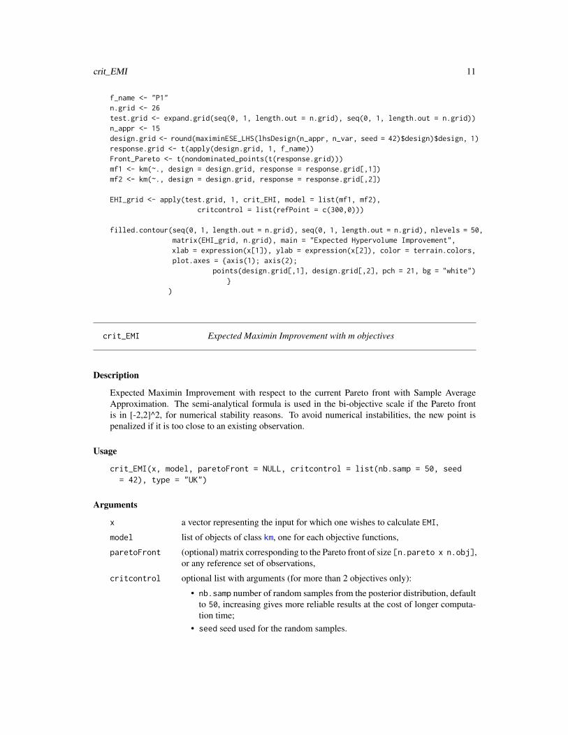
crit_EMI Expected Maximin Improvement with m objectives

Description

Expected Maximin Improvement with respect to the current Pareto front with Sample AverageApproximation. The semi-analytical formula is used in the bi-objective scale if the Pareto frontis in [-2,2]^2, for numerical stability reasons. To avoid numerical instabilities, the new point ispenalized if it is too close to an existing observation.

Usage

crit_EMI(x, model, paretoFront = NULL, critcontrol = list(nb.samp = 50, seed= 42), type = "UK")

Arguments

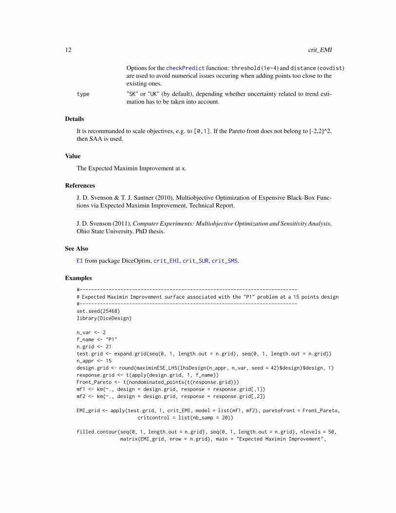
x a vector representing the input for which one wishes to calculate EMI,



critcontrol optional list with arguments (for more than 2 objectives only):

• nb.samp number of random samples from the posterior distribution, defaultto 50, increasing gives more reliable results at the cost of longer computa-tion time;

• seed seed used for the random samples.

12 crit_EMI



Details

It is recommanded to scale objectives, e.g. to [0,1]. If the Pareto front does not belong to [-2,2]^2,then SAA is used.

Value

The Expected Maximin Improvement at x.

References

J. D. Svenson & T. J. Santner (2010), Multiobjective Optimization of Expensive Black-Box Func-tions via Expected Maximin Improvement, Technical Report.

J. D. Svenson (2011), Computer Experiments: Multiobjective Optimization and Sensitivity Analysis,Ohio State University, PhD thesis.

See Also

EI from package DiceOptim, crit_EHI, crit_SUR, crit_SMS.

Examples

#---------------------------------------------------------------------------# Expected Maximin Improvement surface associated with the "P1" problem at a 15 points design#---------------------------------------------------------------------------set.seed(25468)library(DiceDesign)

n_var <- 2f_name <- "P1"n.grid <- 21test.grid <- expand.grid(seq(0, 1, length.out = n.grid), seq(0, 1, length.out = n.grid))n_appr <- 15design.grid <- round(maximinESE_LHS(lhsDesign(n_appr, n_var, seed = 42)$design)$design, 1)response.grid <- t(apply(design.grid, 1, f_name))Front_Pareto <- t(nondominated_points(t(response.grid)))mf1 <- km(~., design = design.grid, response = response.grid[,1])mf2 <- km(~., design = design.grid, response = response.grid[,2])

EMI_grid <- apply(test.grid, 1, crit_EMI, model = list(mf1, mf2), paretoFront = Front_Pareto,critcontrol = list(nb_samp = 20))

filled.contour(seq(0, 1, length.out = n.grid), seq(0, 1, length.out = n.grid), nlevels = 50,matrix(EMI_grid, nrow = n.grid), main = "Expected Maximin Improvement",

crit_optimizer 13

xlab = expression(x[1]), ylab = expression(x[2]), color = terrain.colors,plot.axes = {axis(1); axis(2);


)

crit_optimizer Maximization of multiobjective Expected Improvement criteria

Description

Given a list of objects of class km and a set of tuning parameters (lower, upper and critcontrol),crit_optimizer performs the maximization of an Expected Improvement or SUR criterion and de-livers the next point to be visited in a multi-objective EGO-like procedure.

The latter maximization relies either on a genetic algorithm using derivatives, genoud, particleswarm algorithm pso, exhaustive search at pre-specified points or on a user defined method. It isimportant to remark that the information needed about the objective function reduces here to thevector of response values embedded in the models (no call to the objective functions or simulators(except with cheapfn)).

Usage

crit_optimizer(crit = "SMS", model, lower, upper, cheapfn = NULL,type = "UK", paretoFront = NULL, critcontrol = NULL,optimcontrol = NULL)

Arguments

crit sampling criterion. Four choices are available : "SMS", "EHI", "EMI" and "SUR",


lower vector of lower bounds for the variables to be optimized over,

upper vector of upper bounds for the variables to be optimized over,

cheapfn optional additional fast-to-evaluate objective function (handled next with classfastfun), which does not need a kriging model,



critcontrol optional list of control parameters for criterion crit, see details. Options for thecheckPredict function: threshold (1e-4) and distance (covdist) are usedto avoid numerical issues occuring when adding points too close to the existingones.

14 crit_optimizer

optimcontrol optional list of control parameters for optimization of the selected infill criterion."method" set the optimization method; one can choose between "discrete","pso" and "genoud" or a user defined method name (passed to match.fun). Foreach method, further parameters can be set.For "discrete", one has to provide the argument "candidate.points".For "pso", one can control the maximum number of iterations "maxit" (400) andthe population size "s" (default : max(20, floor(10+2*sqrt(length(dim))))(see psoptim).For "genoud", one can control, among others, "pop.size" (default : [N = 3*2^dimfor dim < 6 and N = 32*dim otherwise]), "max.generations" (12), "wait.generations"(2), "BFGSburnin" (2), BFGSmaxit (N) and solution.tolerance (1e-21) offunction "genoud" (see genoud). Numbers into brackets are the default values.For a user defined method, it must have arguments like the default optim method,i.e. par, fn, lower, upper, ... and possibly control, and return a list with parand value. A trace trace argument is available, it can be set to 0 to suppress allmessages, to 1 (default) for displaying the optimization progresses, and >1 forthe highest level of details.

Details

Extension of the function max_EI for multi-objective optimization.Available infill criteria with crit are :

• Expected Hypervolume Improvement (EHI) crit_EHI,

• SMS criterion (SMS) crit_SMS,

• Expected Maximin Improvement (EMI) crit_EMI,

• Stepwise Uncertainty Reduction of the excursion volume (SUR) crit_SUR

Depending on the selected criterion, parameters such as a reference point for SMS and EHI or ar-guments for integration_design_optim with SUR can be given with critcontrol. Also optionsfor checkPredict are available. More precisions are given in the corresponding help pages.

Value

A list with components:

• par: The best set of parameters found,

• value: The value of expected improvement at par.

References

W.R. Jr. Mebane and J.S. Sekhon (2011), Genetic optimization using derivatives: The rgenoudpackage for R, Journal of Statistical Software, 42(11), 1-26

D.R. Jones, M. Schonlau, and W.J. Welch (1998), Efficient global optimization of expensive black-box functions, Journal of Global Optimization, 13, 455-492.

crit_optimizer 15

Examples

## Not run:#---------------------------------------------------------------------------# EHI surface associated with the "P1" problem at a 15 points design#---------------------------------------------------------------------------

set.seed(25468)library(DiceDesign)

d <- 2n.obj <- 2fname <- "P1"n.grid <- 51test.grid <- expand.grid(seq(0, 1, length.out = n.grid), seq(0, 1, length.out = n.grid))nappr <- 15design.grid <- round(maximinESE_LHS(lhsDesign(nappr, d, seed = 42)$design)$design, 1)response.grid <- t(apply(design.grid, 1, fname))paretoFront <- t(nondominated_points(t(response.grid)))mf1 <- km(~., design = design.grid, response = response.grid[,1])mf2 <- km(~., design = design.grid, response = response.grid[,2])model <- list(mf1, mf2)

EHI_grid <- apply(test.grid, 1, crit_EHI, model = list(mf1, mf2),critcontrol = list(refPoint = c(300, 0)))

lower <- rep(0, d)upper <- rep(1, d)

omEGO <- crit_optimizer(crit = "EHI", model = model, lower = lower, upper = upper,optimcontrol = list(method = "genoud", pop.size = 200, BFGSburnin = 2),critcontrol = list(refPoint = c(300, 0)))

print(omEGO)

filled.contour(seq(0, 1, length.out = n.grid), seq(0, 1, length.out = n.grid), nlevels = 50,matrix(EHI_grid, nrow = n.grid), main = "Expected Hypervolume Improvement",xlab = expression(x[1]), ylab = expression(x[2]), color = terrain.colors,plot.axes = {axis(1); axis(2);

points(design.grid[, 1], design.grid[, 2], pch = 21, bg = "white");points(omEGO$par, col = "red", pch = 4)}

)

#---------------------------------------------------------------------------# SMS surface associated with the "P1" problem at a 15 points design#---------------------------------------------------------------------------

SMS_grid <- apply(test.grid, 1, crit_SMS, model = model,critcontrol = list(refPoint = c(300, 0)))

lower <- rep(0, d)

16 crit_optimizer

upper <- rep(1, d)

omEGO2 <- crit_optimizer(crit = "SMS", model = model, lower = lower, upper = upper,optimcontrol = list(method="genoud", pop.size = 200, BFGSburnin = 2),critcontrol = list(refPoint = c(300, 0)))

print(omEGO2)

filled.contour(seq(0, 1, length.out = n.grid), seq(0, 1, length.out = n.grid), nlevels = 50,matrix(pmax(0,SMS_grid), nrow = n.grid), main = "SMS Criterion (>0)",xlab = expression(x[1]), ylab = expression(x[2]), color = terrain.colors,plot.axes = {axis(1); axis(2);

points(design.grid[, 1], design.grid[, 2], pch = 21, bg = "white");points(omEGO2$par, col = "red", pch = 4)}

)#---------------------------------------------------------------------------# Maximin Improvement surface associated with the "P1" problem at a 15 points design#---------------------------------------------------------------------------

EMI_grid <- apply(test.grid, 1, crit_EMI, model = model,critcontrol = list(nb_samp = 20, type ="EMI"))


omEGO3 <- crit_optimizer(crit = "EMI", model = model, lower = lower, upper = upper,optimcontrol = list(method = "genoud", pop.size = 200, BFGSburnin = 2))

print(omEGO3)

filled.contour(seq(0, 1, length.out = n.grid), seq(0, 1, length.out = n.grid), nlevels = 50,matrix(EMI_grid, nrow = n.grid), main = "Expected Maximin Improvement",xlab = expression(x[1]), ylab = expression(x[2]), color = terrain.colors,plot.axes = {axis(1);axis(2);

points(design.grid[, 1], design.grid[, 2], pch = 21, bg = "white");points(omEGO3$par, col = "red", pch = 4)}

)#---------------------------------------------------------------------------# crit_SUR surface associated with the "P1" problem at a 15 points design#---------------------------------------------------------------------------library(KrigInv)

integration.param <- integration_design_optim(lower = c(0, 0), upper = c(1, 1), model = model)integration.points <- as.matrix(integration.param$integration.points)integration.weights <- integration.param$integration.weights

precalc.data <- list()mn.X <- sn.X <- matrix(0, n.obj, nrow(integration.points))

for (i in 1:n.obj){

crit_optimizer 17

p.tst.all <- predict(model[[i]], newdata = integration.points, type = "UK",checkNames = FALSE)

mn.X[i,] <- p.tst.all$meansn.X[i,] <- p.tst.all$sdprecalc.data[[i]] <- precomputeUpdateData(model[[i]], integration.points)

}critcontrol <- list(integration.points = integration.points,

integration.weights = integration.weights,mn.X = mn.X, sn.X = sn.X, precalc.data = precalc.data)

EEV_grid <- apply(test.grid, 1, crit_SUR, model=model, paretoFront = paretoFront,critcontrol = critcontrol)


omEGO4 <- crit_optimizer(crit = "SUR", model = model, lower = lower, upper = upper,optimcontrol = list(method = "genoud", pop.size = 200, BFGSburnin = 2))

print(omEGO4)

filled.contour(seq(0, 1, length.out = n.grid), seq(0, 1, length.out = n.grid),matrix(pmax(0,EEV_grid), n.grid), main = "EEV criterion", nlevels = 50,xlab = expression(x[1]), ylab = expression(x[2]), color = terrain.colors,plot.axes = {axis(1); axis(2);

points(design.grid[,1], design.grid[,2], pch = 21, bg = "white")points(omEGO4$par, col = "red", pch = 4)}

)

# example using user defined optimizer, here L-BFGS-B from base optimuserOptim <- function(par, fn, lower, upper, control, ...){

return(optim(par = par, fn = fn, method = "L-BFGS-B", lower = lower, upper = upper,control = control, ...))

}omEGO4bis <- crit_optimizer(crit = "SUR", model = model, lower = lower, upper = upper,

optimcontrol = list(method = "userOptim"))print(omEGO4bis)

#---------------------------------------------------------------------------# crit_SMS surface with problem "P1" with 15 design points, using cheapfn#---------------------------------------------------------------------------

# Optimization with fastfun: SMS with discrete search# Separation of the problem P1 in two objectives:# the first one to be kriged, the second one with fastobj

# Definition of the fastfunf2 <- function(x){

return(P1(x)[2])}

SMS_grid_cheap <- apply(test.grid, 1, crit_SMS, model = list(mf1, fastfun(f2, design.grid)),paretoFront = paretoFront, critcontrol = list(refPoint = c(300, 0)))

18 crit_SMS

optimcontrol <- list(method = "pso")model2 <- list(mf1)omEGO5 <- crit_optimizer(crit = "SMS", model = model2, lower = lower, upper = upper,

cheapfn = f2, critcontrol = list(refPoint = c(300, 0)),optimcontrol = list(method = "genoud", pop.size = 200, BFGSburnin = 2))

print(omEGO5)

filled.contour(seq(0, 1, length.out = n.grid), seq(0, 1, length.out = n.grid),matrix(pmax(0, SMS_grid_cheap), nrow = n.grid), nlevels = 50,

main = "SMS criterion with cheap 2nd objective (>0)", xlab = expression(x[1]),ylab = expression(x[2]), color = terrain.colors,plot.axes = {axis(1); axis(2);

points(design.grid[,1], design.grid[,2], pch = 21, bg = "white")points(omEGO5$par, col = "red", pch = 4)}

)

## End(Not run)

crit_SMS Analytical expression of the SMS-EGO criterion with m>1 objectives

Description

Computes a slightly modified infill Criterion of the SMS-EGO. To avoid numerical instabilities, anadditional penalty is added to the new point if it is too close to an existing observation.

Usage

crit_SMS(x, model, paretoFront = NULL, critcontrol = NULL, type = "UK")

Arguments

x a vector representing the input for which one wishes to calculate the criterion,

model a list of objects of class km (one for each objective),


critcontrol list with arguments:

• currentHV current hypervolume;• refPoint reference point for hypervolume computations;• extendper if no reference point refPoint is provided, for each objective

it is fixed to the maximum over the Pareto front plus extendper times therange. Default value to 0.2, corresponding to 1.1 for a scaled objectivewith a Pareto front in [0,1]^n.obj;

• epsilon optional value to use in additive epsilon dominance;• gain optional gain factor for sigma.

crit_SMS 19



Value

Value of the criterion.

References

W. Ponweiser, T. Wagner, D. Biermann, M. Vincze (2008), Multiobjective Optimization on a Lim-ited Budget of Evaluations Using Model-Assisted S-Metric Selection, Parallel Problem Solvingfrom Nature, pp. 784-794. Springer, Berlin.

T. Wagner, M. Emmerich, A. Deutz, W. Ponweiser (2010), On expected-improvement criteria formodel-based multi-objective optimization. Parallel Problem Solving from Nature, pp. 718-727.Springer, Berlin.

See Also

crit_EHI, crit_SUR, crit_EMI.

Examples

#---------------------------------------------------------------------------# SMS-EGO surface associated with the "P1" problem at a 15 points design#---------------------------------------------------------------------------set.seed(25468)library(DiceDesign)

n_var <- 2f_name <- "P1"n.grid <- 26test.grid <- expand.grid(seq(0, 1, length.out = n.grid), seq(0, 1, length.out = n.grid))n_appr <- 15design.grid <- round(maximinESE_LHS(lhsDesign(n_appr, n_var, seed = 42)$design)$design, 1)response.grid <- t(apply(design.grid, 1, f_name))PF <- t(nondominated_points(t(response.grid)))mf1 <- km(~., design = design.grid, response = response.grid[,1])mf2 <- km(~., design = design.grid, response = response.grid[,2])

model <- list(mf1, mf2)critcontrol <- list(refPoint = c(300, 0), currentHV = dominated_hypervolume(t(PF), c(300, 0)))SMSEGO_grid <- apply(test.grid, 1, crit_SMS, model = model,

paretoFront = PF, critcontrol = critcontrol)

filled.contour(seq(0, 1, length.out = n.grid), seq(0, 1, length.out = n.grid),matrix(pmax(0, SMSEGO_grid), nrow = n.grid), nlevels = 50,main = "SMS-EGO criterion (positive part)", xlab = expression(x[1]),

20 crit_SUR

ylab = expression(x[2]), color = terrain.colors,plot.axes = {axis(1); axis(2);

points(design.grid[,1],design.grid[,2], pch = 21, bg = "white")}

)

crit_SUR Analytical expression of the SUR criterion for two or three objectives.

Description

Computes the SUR criterion (Expected Excursion Volume Reduction) at point x for 2 or 3 objec-tives. To avoid numerical instabilities, the new point is penalized if it is too close to an existingobservation.

Usage

crit_SUR(x, model, paretoFront = NULL, critcontrol = NULL, type = "UK")

Arguments

x a vector representing the input for which one wishes to calculate the criterion,

model a list of objects of class km (one for each objective),


critcontrol list with two possible options.

A) One can use the four following arguments:

• integration.points, matrix of integration points of size [n.integ.pts x d];• integration.weights, vector of integration weights of length n.integ.pts;• mn.X and sn.X, matrices of kriging means and sd, each of size [n.obj x n.integ.pts];• precalc.data, list of precalculated data (based on kriging models at inte-

gration points) for faster computation.

B) Alternatively, one can define arguments passed to integration_design_optim:SURcontrol (optional), lower, upper, min.prob (optional). This is slowersince arguments of A), used in the function, are then recomputed each time (notethat this is not the case when called from GParetoptim and crit_optimizer).



crit_SUR 21

Value

Value of the criterion.

References

V. Picheny (2014), Multiobjective optimization using Gaussian process emulators via stepwise un-certainty reduction, Statistics and Computing.

See Also

crit_EHI, crit_SMS, crit_EMI.

Examples

#---------------------------------------------------------------------------# crit_SUR surface associated with the "P1" problem at a 15 points design#---------------------------------------------------------------------------set.seed(25468)library(DiceDesign)library(KrigInv)

n_var <- 2n.obj <- 2f_name <- "P1"n.grid <- 14test.grid <- expand.grid(seq(0, 1, length.out = n.grid), seq(0, 1, length.out = n.grid))n_appr <- 15design.grid <- round(maximinESE_LHS(lhsDesign(n_appr, n_var, seed = 42)$design)$design, 1)response.grid <- t(apply(design.grid, 1, f_name))paretoFront <- t(nondominated_points(t(response.grid)))mf1 <- km(~., design = design.grid, response = response.grid[,1])mf2 <- km(~., design = design.grid, response = response.grid[,2])

model <- list(mf1, mf2)

integration.param <- integration_design_optim(lower = c(0, 0), upper = c(1, 1), model = model)integration.points <- as.matrix(integration.param$integration.points)integration.weights <- integration.param$integration.weights

precalc.data <- list()mn.X <- sn.X <- matrix(0, nrow = n.obj, ncol = nrow(integration.points))

for (i in 1:n.obj){p.tst.all <- predict(model[[i]], newdata = integration.points, type = "UK", checkNames = FALSE)mn.X[i,] <- p.tst.all$meansn.X[i,] <- p.tst.all$sdprecalc.data[[i]] <- precomputeUpdateData(model[[i]], integration.points)

}

critcontrol <- list(integration.points = integration.points,integration.weights = integration.weights,

22 easyGParetoptim

mn.X = mn.X, sn.X = sn.X, precalc.data = precalc.data)## Alternatively: critcontrol <- list(lower = rep(0, n_var), upper = rep(1,n_var))

EEV_grid <- apply(test.grid, 1, crit_SUR, model = model, paretoFront = paretoFront,critcontrol = critcontrol)

filled.contour(seq(0, 1, length.out = n.grid), seq(0, 1, length.out = n.grid),matrix(pmax(0,EEV_grid), nrow = n.grid), main = "EEV criterion",xlab = expression(x[1]), ylab = expression(x[2]), color = terrain.colors,plot.axes = {axis(1); axis(2);


)

easyGParetoptim EGO algorithm for multiobjective optimization

Description

User-friendly wrapper of the function GParetoptim. Generates initial DOEs and kriging models(objects of class km), and executes nsteps iterations of multiobjective EGO methods.

Usage

easyGParetoptim(fn, cheapfn = NULL, budget, lower, upper, par = NULL,value = NULL, noise.var = NULL, control = list(method = "SMS", trace =1, inneroptim = "pso", maxit = 100, seed = 42), ...)

Arguments

fn the multi-objective function to be minimized (vectorial output), found by a callto match.fun, see details,

cheapfn optional additional fast-to-evaluate objective function (handled next with classfastfun), which does not need a kriging model, handled by a call to match.fun,

budget total number of calls to the objective function,



par initial design of experiments. If not provided, par is taken as a maximin LHDwith budget/3 points,

value initial set of objective observations fn(par). Computed if not provided. Notthat value may NOT contain any cheapfn value,

noise.var optional noise variance, for noisy objectives fn. If not NULL, either a scalar(constant noise, identical for all objectives), a vector (constant noise, differentfor each objective) or a function (type closure) with vectorial output (variablenoise, different for each objective). Alternatively, set noise.var="given_by_fn",see details.

easyGParetoptim 23

control an optional list of control parameters. See "Details",

... additional parameters to be given to the objective fn.

Details

Does not require specific knowledge on kriging models (objects of class km).

The problem considered is of the form: minf(x) = f1(x), ..., fp(x). The control argument is alist that can supply any of the following optional components:

• method: choice of multiobjective improvement function: "SMS", "EHI", "EMI" or "SUR" (seecrit_SMS, crit_EHI, crit_EMI, crit_SUR),

• trace: if positive, tracing information on the progress of the optimization is produced (1(default) for general progress, >1 for more details, e.g., warnings from genoud),

• inneroptim: choice of the inner optimization algorithm: "genoud", "pso" or "random" (seegenoud and psoptim),

• maxit: maximum number of iterations of the inner loop,

• seed: to fix the random variable generator,

• refPoint: reference point for hypervolume computations (for "SMS" and "EHI" methods),

• extendper: if no reference point refPoint is provided, for each objective it is fixed to themaximum over the Pareto front plus extendper times the range. Default value to 0.2, corre-sponding to 1.1 for a scaled objective with a Pareto front in [0,1]^n.obj.

If noise.var="given_by_fn", fn must return a list of two vectors, the first being the objectivefunctions and the second the corresponding noise variances. See examples in GParetoptim.

For additional details or other possible arguments, see GParetoptim.

Display of results and various post-processings are available with plotGPareto.

Value


• par: all the non-dominated points found,

• value: the matrix of objective values at the points given in par,

• history: a list containing all the points visited by the algorithm (X) and their correspondingobjectives (y),

• model: a list of objects of class km, corresponding to the last kriging models fitted.

Note that in the case of noisy problems, value and history$y.denoised are denoised values. Theoriginal observations are available in the slot history$y.

Author(s)

Victor Picheny (INRA, Castanet-Tolosan, France)

Mickael Binois (Mines Saint-Etienne/Renault, France)

24 easyGParetoptim

References


V. Picheny (2015), Multiobjective optimization using Gaussian process emulators via stepwise un-certainty reduction, Statistics and Computing, 25(6), 1265-1280.

T. Wagner, M. Emmerich, A. Deutz, W. Ponweiser (2010), On expected-improvement criteriafor model-based multi-objective optimization. Parallel Problem Solving from Nature, 718-727,Springer, Berlin.

J. D. Svenson (2011), Computer Experiments: Multiobjective Optimization and Sensitivity Anal-ysis, Ohio State university, PhD thesis.

Examples

#---------------------------------------------------------------------------# 2D objective function, 4 cases#---------------------------------------------------------------------------## Not run:set.seed(25468)n_var <- 2fname <- ZDT3lower <- rep(0, n_var)upper <- rep(1, n_var)

#---------------------------------------------------------------------------# 1- Expected Hypervolume Improvement optimization, using pso#---------------------------------------------------------------------------res <- easyGParetoptim(fn=fname, lower=lower, upper=upper, budget=15,

control=list(method="EHI", inneroptim="pso", maxit=20))par(mfrow=c(1,2))plotGPareto(res)title("Pareto Front")plot(res$history$X, main="Pareto set", col = "red", pch = 20)points(res$par, col="blue", pch = 17)

#---------------------------------------------------------------------------# 2- SMS Improvement optimization using random search, with initial DOE given#---------------------------------------------------------------------------library(DiceDesign)design.init <- maximinESE_LHS(lhsDesign(10, n_var, seed = 42)$design)$designresponse.init <- t(apply(design.init, 1, fname))res <- easyGParetoptim(fn=fname, par=design.init, value=response.init, lower=lower, upper=upper,

budget=15, control=list(method="SMS", inneroptim="random", maxit=100))par(mfrow=c(1,2))plotGPareto(res)title("Pareto Front")plot(res$history$X, main="Pareto set", col = "red", pch = 20)points(res$par, col="blue", pch = 17)

fastfun 25

#---------------------------------------------------------------------------# 3- Stepwise Uncertainty Reduction optimization, with one fast objective function#---------------------------------------------------------------------------fname <- camelbackcheapfn <- function(x) {if (is.null(dim(x))) return(-sum(x))else return(-rowSums(x))}res <- easyGParetoptim(fn=fname, cheapfn=cheapfn, lower=lower, upper=upper, budget=15,

control=list(method="SUR", inneroptim="pso", maxit=20))par(mfrow=c(1,2))plotGPareto(res)title("Pareto Front")plot(res$history$X, main="Pareto set", col = "red", pch = 20)points(res$par, col="blue", pch = 17)

#---------------------------------------------------------------------------# 4- Expected Hypervolume Improvement optimization, using pso, noisy fn#---------------------------------------------------------------------------noise.var <- c(0.1, 0.2)funnoise <- function(x) {ZDT3(x) + sqrt(noise.var)*rnorm(n=2)}res <- easyGParetoptim(fn=funnoise, lower=lower, upper=upper, budget=30, noise.var=noise.var,

control=list(method="EHI", inneroptim="pso", maxit=20))par(mfrow=c(1,2))plotGPareto(res)title("Pareto Front")plot(res$history$X, main="Pareto set", col = "red", pch = 20)points(res$par, col="blue", pch = 17)

#---------------------------------------------------------------------------# 5- Stepwise Uncertainty Reduction optimization, functional noise#---------------------------------------------------------------------------funnoise <- function(x) {ZDT3(x) + sqrt(abs(0.1*x))*rnorm(n=2)}noise.var <- function(x) return(abs(0.1*x))

res <- easyGParetoptim(fn=funnoise, lower=lower, upper=upper, budget=30, noise.var=noise.var,control=list(method="SUR", inneroptim="pso", maxit=20))

par(mfrow=c(1,2))plotGPareto(res)title("Pareto Front")plot(res$history$X, main="Pareto set", col = "red", pch = 20)points(res$par, col="blue", pch = 17)

## End(Not run)

fastfun Fast-to-evaluate function wrapper

26 fastfun

Description

Modification of an R function to be used with methods predict and update (similar to a km ob-ject). It creates an S4 object which contains the values corresponding to evaluations of other costlyobservations. It is useful when an objective can be evaluated fast.

Usage

fastfun(fn, design, response = NULL)

Arguments

fn the evaluator function, found by a call to match.fun,

design a data frame representing the design of experiments. The ith row contains thevalues of the d input variables corresponding to the ith evaluation.

response optional vector (or 1-column matrix or data frame) containing the values of the1-dimensional output given by the objective function at the design points.

Value

An object of class fastfun-class.

Examples

########################################################## Example with a fast to evaluate objective########################################################## Not run:set.seed(25468)library(DiceDesign)

d <- 2

fname <- P1n.grid <- 21nappr <- 11design.grid <- maximinESE_LHS(lhsDesign(nappr, d, seed = 42)$design)$designresponse.grid <- t(apply(design.grid, 1, fname))Front_Pareto <- t(nondominated_points(t(response.grid)))

mf1 <- km(~., design = design.grid, response = response.grid[,1])mf2 <- km(~., design = design.grid, response = response.grid[,2])model <- list(mf1, mf2)


# Optimization reference: SMS with discrete searchoptimcontrol <- list(method = "pso")omEGO1 <- GParetoptim(model = model, fn = fname, crit = "SMS", nsteps = nsteps,

lower = lower, upper = upper, optimcontrol = optimcontrol)

getDesign 27

print(omEGO1$par)print(omEGO1$values)plot(response.grid, xlim = c(0,300), ylim = c(-40,0), pch = 17, col = "blue")points(omEGO1$values, pch = 20, col ="green")

# Optimization with fastfun: SMS with discrete search# Separation of the problem P1 in two objectives:# the first one to be kriged, the second one with fastobjf1 <- function(x){

if(is.null(dim(x))) x <- matrix(x, nrow = 1)b1 <- 15*x[,1] - 5b2 <- 15*x[,2]return( (b2 - 5.1*(b1/(2*pi))^2 + 5/pi*b1 - 6)^2 +10*((1 - 1/(8*pi))*cos(b1) + 1))

}

f2 <- function(x){if(is.null(dim(x))) x <- matrix(x, nrow = 1)b1<-15*x[,1] - 5b2<-15*x[,2]return(-sqrt((10.5 - b1)*(b1 + 5.5)*(b2 + 0.5))

- 1/30*(b2 - 5.1*(b1/(2*pi))^2 - 6)^2- 1/3*((1 - 1/(8*pi))*cos(b1) + 1))

}

optimcontrol <- list(method = "pso")model2 <- list(mf1)omEGO2 <- GParetoptim(model = model2, fn = f1, cheapfn = f2, crit = "SMS", nsteps = nsteps,

lower = lower, upper = upper, optimcontrol = optimcontrol)print(omEGO2$par)print(omEGO2$values)

points(omEGO2$values, col = "red", pch = 15)

## End(Not run)

getDesign Get design corresponding to an objective target

Description

Find the design that maximizes the probability of dominating a target given by the user.

Usage

getDesign(model, target, lower, upper, optimcontrol = NULL)

Arguments


target vector corresponding to the desired output in the objective space,

28 getDesign



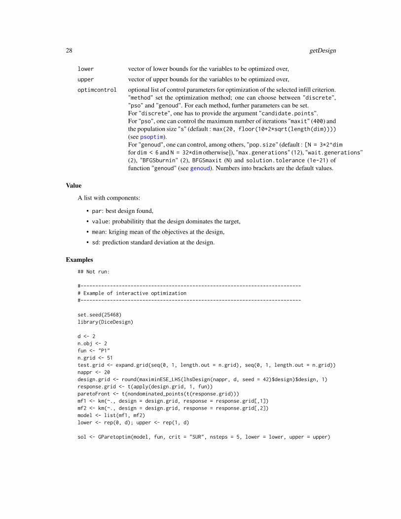
optimcontrol optional list of control parameters for optimization of the selected infill criterion."method" set the optimization method; one can choose between "discrete","pso" and "genoud". For each method, further parameters can be set.For "discrete", one has to provide the argument "candidate.points".For "pso", one can control the maximum number of iterations "maxit" (400) andthe population size "s" (default : max(20, floor(10+2*sqrt(length(dim))))(see psoptim).For "genoud", one can control, among others, "pop.size" (default : [N = 3*2^dimfor dim < 6 and N = 32*dim otherwise]), "max.generations" (12), "wait.generations"(2), "BFGSburnin" (2), BFGSmaxit (N) and solution.tolerance (1e-21) offunction "genoud" (see genoud). Numbers into brackets are the default values.

Value


• par: best design found,

• value: probabilitity that the design dominates the target,

• mean: kriging mean of the objectives at the design,

• sd: prediction standard deviation at the design.

Examples

## Not run:

#---------------------------------------------------------------------------# Example of interactive optimization#---------------------------------------------------------------------------


d <- 2n.obj <- 2fun <- "P1"n.grid <- 51test.grid <- expand.grid(seq(0, 1, length.out = n.grid), seq(0, 1, length.out = n.grid))nappr <- 20design.grid <- round(maximinESE_LHS(lhsDesign(nappr, d, seed = 42)$design)$design, 1)response.grid <- t(apply(design.grid, 1, fun))paretoFront <- t(nondominated_points(t(response.grid)))mf1 <- km(~., design = design.grid, response = response.grid[,1])mf2 <- km(~., design = design.grid, response = response.grid[,2])model <- list(mf1, mf2)lower <- rep(0, d); upper <- rep(1, d)

sol <- GParetoptim(model, fun, crit = "SUR", nsteps = 5, lower = lower, upper = upper)

GParetoptim 29

plotGPareto(sol)

target1 <- c(15, -25)points(x = target1[1], y = target1[2], col = "black", pch = 13)

nDesign <- getDesign(sol$lastmodel, target = target1, lower = rep(0, d), upper = rep(1, d))points(t(nDesign$mean), col = "green", pch = 20)

target2 <- c(48, -27)points(x = target2[1], y = target2[2], col = "black", pch = 13)nDesign2 <- getDesign(sol$lastmodel, target = target2, lower = rep(0, d), upper = rep(1, d))points(t(nDesign2$mean), col = "darkgreen", pch = 20)

## End(Not run)

GParetoptim Sequential multi-objective Expected Improvement maximization andmodel re-estimation, with a number of iterations fixed in advance bythe user

Description

Executes nsteps iterations of multi-objective EGO methods to objects of class km. At each step,kriging models are re-estimated (including covariance parameters re-estimation) based on the initialdesign points plus the points visited during all previous iterations; then a new point is obtainedby maximizing one of the four multi-objective Expected Improvement criteria available. Handlesnoiseless and noisy objective functions.

Usage

GParetoptim(model, fn, cheapfn = NULL, crit = "SMS", nsteps, lower, upper,type = "UK", cov.reestim = TRUE, critcontrol = NULL, noise.var = NULL,reinterpolation = NULL, optimcontrol = list(method = "genoud", trace = 1),...)

Arguments


fn the multi-objective function to be minimized (vectorial output), found by a callto match.fun,

cheapfn optional additional fast-to-evaluate objective function (handled next with classfastfun), which does not need a kriging model, handled by a call to match.fun,

crit choice of multi-objective improvement function: "SMS", "EHI", "EMI" or "SUR",see details below,

nsteps an integer representing the desired number of iterations,



30 GParetoptim

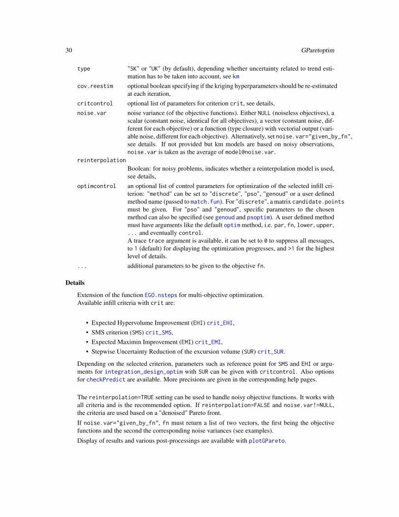
type "SK" or "UK" (by default), depending whether uncertainty related to trend esti-mation has to be taken into account, see km

cov.reestim optional boolean specifying if the kriging hyperparameters should be re-estimatedat each iteration,

critcontrol optional list of parameters for criterion crit, see details,noise.var noise variance (of the objective functions). Either NULL (noiseless objectives), a

scalar (constant noise, identical for all objectives), a vector (constant noise, dif-ferent for each objective) or a function (type closure) with vectorial output (vari-able noise, different for each objective). Alternatively, set noise.var="given_by_fn",see details. If not provided but km models are based on noisy observations,noise.var is taken as the average of [email protected].

reinterpolation

Boolean: for noisy problems, indicates whether a reinterpolation model is used,see details,

optimcontrol an optional list of control parameters for optimization of the selected infill cri-terion: "method" can be set to "discrete", "pso", "genoud" or a user definedmethod name (passed to match.fun). For "discrete", a matrix candidate.pointsmust be given. For "pso" and "genoud", specific parameters to the chosenmethod can also be specified (see genoud and psoptim). A user defined methodmust have arguments like the default optim method, i.e. par, fn, lower, upper,... and eventually control.A trace trace argument is available, it can be set to 0 to suppress all messages,to 1 (default) for displaying the optimization progresses, and >1 for the highestlevel of details.

... additional parameters to be given to the objective fn.

Details

Extension of the function EGO.nsteps for multi-objective optimization.Available infill criteria with crit are:

• Expected Hypervolume Improvement (EHI) crit_EHI,• SMS criterion (SMS) crit_SMS,• Expected Maximin Improvement (EMI) crit_EMI,• Stepwise Uncertainty Reduction of the excursion volume (SUR) crit_SUR.

Depending on the selected criterion, parameters such as reference point for SMS and EHI or argu-ments for integration_design_optim with SUR can be given with critcontrol. Also optionsfor checkPredict are available. More precisions are given in the corresponding help pages.

The reinterpolation=TRUE setting can be used to handle noisy objective functions. It works withall criteria and is the recommended option. If reinterpolation=FALSE and noise.var!=NULL,the criteria are used based on a "denoised" Pareto front.

If noise.var="given_by_fn", fn must return a list of two vectors, the first being the objectivefunctions and the second the corresponding noise variances (see examples).

Display of results and various post-processings are available with plotGPareto.

GParetoptim 31

Value


• par: a data frame representing the additional points visited during the algorithm,

• values: a data frame representing the response values at the points given in par,

• nsteps: an integer representing the desired number of iterations (given in argument),

• lastmodel: a list of objects of class km corresponding to the last kriging models fitted.

• observations.denoised: if noise.var!=NULL, a matrix representing the mean values of thekm models at observation points. If a problem occurs during either model updates or criterionmaximization, the last working model and corresponding values are returned.

References


V. Picheny (2014), Multiobjective optimization using Gaussian process emulators via stepwise un-certainty reduction, Statistics and Computing, 25(6), 1265-1280

T. Wagner, M. Emmerich, A. Deutz, W. Ponweiser (2010), On expected-improvement criteriafor model-based multi-objective optimization. Parallel Problem Solving from Nature, 718-727,Springer, Berlin.

J. D. Svenson (2011), Computer Experiments: Multiobjective Optimization and Sensitivity Anal-ysis, Ohio State university, PhD thesis. V. Picheny and D. Ginsbourger (2013), Noisy kriging-basedoptimization methods: A unified implementation within the DiceOptim package, ComputationalStatistics & Data Analysis, 71: 1035-1053.

Examples


################################################# NOISELESS PROBLEMS################################################d <- 2fname <- ZDT3n.grid <- 21test.grid <- expand.grid(seq(0, 1, length.out = n.grid), seq(0, 1, length.out = n.grid))nappr <- 15design.grid <- maximinESE_LHS(lhsDesign(nappr, d, seed = 42)$design)$designresponse.grid <- t(apply(design.grid, 1, fname))Front_Pareto <- t(nondominated_points(t(response.grid)))

mf1 <- km(~1, design = design.grid, response = response.grid[, 1], lower=c(.1,.1))mf2 <- km(~., design = design.grid, response = response.grid[, 2], lower=c(.1,.1))model <- list(mf1, mf2)

32 GParetoptim


# Optimization 1: EHI with psooptimcontrol <- list(method = "pso", maxit = 20)critcontrol <- list(refPoint = c(1, 10))omEGO1 <- GParetoptim(model = model, fn = fname, crit = "EHI", nsteps = nsteps,

lower = lower, upper = upper, critcontrol = critcontrol,optimcontrol = optimcontrol)


## Not run:nsteps <- 10# Optimization 2: SMS with discrete searchoptimcontrol <- list(method = "discrete", candidate.points = test.grid)critcontrol <- list(refPoint = c(1, 10))omEGO2 <- GParetoptim(model = model, fn = fname, crit = "SMS", nsteps = nsteps,



# Optimization 3: SUR with genoudoptimcontrol <- list(method = "genoud", pop.size = 20, max.generations = 10)critcontrol <- list(distrib = "SUR", n.points = 100)omEGO3 <- GParetoptim(model = model, fn = fname, crit = "SUR", nsteps = nsteps,



# Optimization 4: EMI with psooptimcontrol <- list(method = "pso", maxit = 20)critcontrol <- list(nbsamp = 200)omEGO4 <- GParetoptim(model = model, fn = fname, crit = "EMI", nsteps = nsteps,

lower = lower, upper = upper, optimcontrol = optimcontrol)print(omEGO4$par)print(omEGO4$values)

# graphicssol.grid <- apply(expand.grid(seq(0, 1, length.out = 100),

seq(0, 1, length.out = 100)), 1, fname)plot(t(sol.grid), pch = 20, col = rgb(0, 0, 0, 0.05), xlim = c(0, 1),

ylim = c(-2, 10), xlab = expression(f[1]), ylab = expression(f[2]))plotGPareto(res = omEGO1, add = TRUE,

control = list(pch = 20, col = "blue", PF.pch = 17,PF.points.col = "blue", PF.line.col = "blue"))

text(omEGO1$values[,1], omEGO1$values[,2], labels = 1:nsteps, pos = 3, col = "blue")plotGPareto(res = omEGO2, add = TRUE,

control = list(pch = 20, col = "green", PF.pch = 17,

GParetoptim 33

PF.points.col = "green", PF.line.col = "green"))text(omEGO2$values[,1], omEGO2$values[,2], labels = 1:nsteps, pos = 3, col = "green")plotGPareto(res = omEGO3, add = TRUE,

control = list(pch = 20, col = "red", PF.pch = 17,PF.points.col = "red", PF.line.col = "red"))

text(omEGO3$values[,1], omEGO3$values[,2], labels = 1:nsteps, pos = 3, col = "red")plotGPareto(res = omEGO4, add = TRUE,

control = list(pch = 20, col = "orange", PF.pch = 17,PF.points.col = "orange", PF.line.col = "orange"))

text(omEGO4$values[,1], omEGO4$values[,2], labels = 1:nsteps, pos = 3, col = "orange")points(response.grid[,1], response.grid[,2], col = "black", pch = 20)legend("topright", c("EHI", "SMS", "SUR", "EMI"), col = c("blue", "green", "red", "orange"),pch = rep(17,4))

# Post-processingplotGPareto(res = omEGO1, UQ_PF = TRUE, UQ_PS = TRUE, UQ_dens = TRUE)

################################################# NOISY PROBLEMS################################################set.seed(25468)library(DiceDesign)d <- 2nsteps <- 3lower <- rep(0, d)upper <- rep(1, d)optimcontrol <- list(method = "pso", maxit = 20)critcontrol <- list(refPoint = c(1, 10))

n.grid <- 21test.grid <- expand.grid(seq(0, 1, length.out = n.grid), seq(0, 1, length.out = n.grid))n.init <- 30design <- maximinESE_LHS(lhsDesign(n.init, d, seed = 42)$design)$design

fit.models <- function(u) km(~., design = design, response = response[, u],noise.var=design.noise.var[,u])

# Test 1: EHI, constant noise.varnoise.var <- c(0.1, 0.2)funnoise1 <- function(x) {ZDT3(x) + sqrt(noise.var)*rnorm(n=d)}response <- t(apply(design, 1, funnoise1))design.noise.var <- matrix(rep(noise.var, n.init), ncol=d, byrow=TRUE)model <- lapply(1:d, fit.models)

omEGO1 <- GParetoptim(model = model, fn = funnoise1, crit = "EHI", nsteps = nsteps,lower = lower, upper = upper, critcontrol = critcontrol,

reinterpolation=TRUE, noise.var=noise.var, optimcontrol = optimcontrol)plotGPareto(omEGO1)

# Test 2: EMI, noise.var given by fnfunnoise2 <- function(x) {list(ZDT3(x) + sqrt(0.05 + abs(0.1*x))*rnorm(n=d), 0.05 + abs(0.1*x))}temp <- funnoise2(design)

34 GParetoptim

response <- temp[[1]]design.noise.var <- temp[[2]]model <- lapply(1:d, fit.models)

omEGO2 <- GParetoptim(model = model, fn = funnoise2, crit = "EMI", nsteps = nsteps,lower = lower, upper = upper, critcontrol = critcontrol,

reinterpolation=TRUE, noise.var="given_by_fn", optimcontrol = optimcontrol)plotGPareto(omEGO2)

# Test 3: SMS, functional noise.varfunnoise3 <- function(x) {ZDT3(x) + sqrt(0.025 + abs(0.05*x))*rnorm(n=d)}noise.var <- function(x) return(0.025 + abs(0.05*x))response <- t(apply(design, 1, funnoise3))design.noise.var <- t(apply(design, 1, noise.var))model <- lapply(1:d, fit.models)

omEGO3 <- GParetoptim(model = model, fn = funnoise3, crit = "SMS", nsteps = nsteps,lower = lower, upper = upper, critcontrol = critcontrol,

reinterpolation=TRUE, noise.var=noise.var, optimcontrol = optimcontrol)plotGPareto(omEGO3)

# Test 4: SUR, fastfun, constant noise.varnoise.var <- 0.1funnoise4 <- function(x) {ZDT3(x)[1] + sqrt(noise.var)*rnorm(1)}cheapfn <- function(x) ZDT3(x)[2]response <- apply(design, 1, funnoise4)design.noise.var <- rep(noise.var, n.init)model <- list(km(~., design = design, response = response, noise.var=design.noise.var))

omEGO4 <- GParetoptim(model = model, fn = funnoise4, cheapfn = cheapfn, crit = "SUR",nsteps = nsteps, lower = lower, upper = upper, critcontrol = critcontrol,reinterpolation=TRUE, noise.var=noise.var, optimcontrol = optimcontrol)

plotGPareto(omEGO4)

# Test 5: EMI, fastfun, noise.var given by fnfunnoise5 <- function(x) {if (is.null(dim(x))) x <- matrix(x, nrow=1)list(apply(x, 1, ZDT3)[1,] + sqrt(abs(0.05*x[,1]))*rnorm(nrow(x)), abs(0.05*x[,1]))

}

cheapfn <- function(x) {if (is.null(dim(x))) x <- matrix(x, nrow=1)apply(x, 1, ZDT3)[2,]

}

temp <- funnoise5(design)response <- temp[[1]]design.noise.var <- temp[[2]]model <- list(km(~., design = design, response = response, noise.var=design.noise.var))

omEGO5 <- GParetoptim(model = model, fn = funnoise5, cheapfn = cheapfn, crit = "EMI",nsteps = nsteps, lower = lower, upper = upper, critcontrol = critcontrol,reinterpolation=TRUE, noise.var="given_by_fn", optimcontrol = optimcontrol)

integration_design_optim 35

plotGPareto(omEGO5)

# Test 6: EHI, fastfun, functional noise.varnoise.var <- 0.1funnoise6 <- function(x) {ZDT3(x)[1] + sqrt(abs(0.1*x[1]))*rnorm(1)}noise.var <- function(x) return(abs(0.1*x[1]))cheapfn <- function(x) ZDT3(x)[2]response <- apply(design, 1, funnoise6)design.noise.var <- t(apply(design, 1, noise.var))model <- list(km(~., design = design, response = response, noise.var=design.noise.var))

omEGO6 <- GParetoptim(model = model, fn = funnoise6, cheapfn = cheapfn, crit = "EMI",nsteps = nsteps, lower = lower, upper = upper, critcontrol = critcontrol,reinterpolation=TRUE, noise.var=noise.var, optimcontrol = optimcontrol)

plotGPareto(omEGO6)

## End(Not run)

integration_design_optim

Function to build integration points (for the SUR criterion)

Description

Modification of the function integration_design from the package KrigInv to be usable forSUR-based optimization. Handles two or three objectives. Available important sampling schemes:none so far.

Usage

integration_design_optim(SURcontrol = NULL, d = NULL, lower, upper,model = NULL, min.prob = 0.001)

Arguments

SURcontrol Optional list specifying the procedure to build the integration points and weights.Many options are possible; see ’Details’.

d The dimension of the input set. If not provided d is set equal to the length oflower.

lower Vector containing the lower bounds of the design space.

upper Vector containing the upper bounds of the design space.

model A list of kriging models of km class.

min.prob This argument applies only when importance sampling distributions are chosen.For numerical reasons we give a minimum probability for a point to belong tothe importance sample. This avoids probabilities equal to zero and importancesampling weights equal to infinity. In an importance sample of M points, themaximum weight becomes 1/min.prob * 1/M.

36 integration_design_optim

Details

The SURcontrol argument is a list with possible entries integration.points, integration.weights,n.points, n.candidates, distrib, init.distrib and init.distrib.spec. It can be used inone of the three following ways:

• A) If nothing is specified, 100 * d points are chosen using the Sobol sequence;

• B) One can directly set the field integration.points (p * d matrix) for prespecified integra-tion points. In this case these integration points and the corresponding vector integration.weightswill be used for all the iterations of the algorithm;

• C) If the field integration.points is not set then the integration points are renewed at eachiteration. In that case one can control the number of integration points n.points (default:100*d) and a specific distribution distrib. Possible values for distrib are: "sobol", "MC" and"SUR" (default: "sobol"):

– C.1) The choice "sobol" corresponds to integration points chosen with the Sobol se-quence in dimension d (uniform weight);

– C.2) The choice "MC" corresponds to points chosen randomly, uniformly on the domain;– C.3) The choice "SUR" corresponds to importance sampling distributions (unequal weights).

When important sampling procedures are chosen, n.points points are chosen using im-portance sampling among a discrete set of n.candidates points (default: n.points*10)which are distributed according to a distribution init.distrib (default: "sobol"). Pos-sible values for init.distrib are the space filling distributions "sobol" and "MC" or anuser defined distribution "spec". The "sobol" and "MC" choices correspond to quasi ran-dom and random points in the domain. If the "spec" value is chosen the user must fill inmanually the field init.distrib.spec to specify himself a n.candidates * d matrixof points in dimension d.

Value


• integration.points p x d matrix of p points used for the numerical calculation of integrals

• integration.weights a vector of size p corresponding to the weight of each point. If all thepoints are equally weighted, integration.weights is set to NULL

References

V. Picheny (2014), Multiobjective optimization using Gaussian process emulators via stepwise un-certainty reduction, Statistics and Computing.

See Also

GParetoptim crit_SUR integration_design

ParetoSetDensity 37

ParetoSetDensity Estimation of Pareto set density

Description

Estimation of the density of Pareto optimal points in the variable space.

Usage

ParetoSetDensity(model, lower, upper, CPS = NULL, nsim = 50,simpoints = 1000, ...)

Arguments


lower vector of lower bounds for the variables,

upper vector of upper bounds for the variables,

CPS optional matrix containing points from Conditional Pareto Set Simulations (inthe variable space), see details

nsim optional number of conditional simulations to perform if CPS is not provided,

simpoints (optional) If CPS is NULL, either a number of simulation points, or a matrix whereconditional simulations are to be performed. In the first case, then simulationpoints are taken as a maximin LHS design using lhsDesign.

... further arguments to be passed to kde. In particular, if the input dimension isgreater than three, a matrix eval.points can be given (else it is taken as thesimulation points).

Details

This function estimates the density of Pareto optimal points in the variable space given by the sur-rogate models. Based on conditional simulations of the objectives at simulation points, ConditionalPareto Set (CPS) simulations are obtained, out of which a density is fitted.

This function relies on the ks package for the kernel density estimation.

Value

An object of class kde accounting for the estimated density of Pareto optimal points.

Examples

## Not run:#---------------------------------------------------------------------------# Example of estimation of the density of Pareto optimal points#---------------------------------------------------------------------------set.seed(42)n_var <- 2

38 plotGPareto

fname <- P1lower <- rep(0, n_var)upper <- rep(1, n_var)

res1 <- easyGParetoptim(fn = fname, lower = lower, upper = upper, budget = 15,control=list(method = "EHI", inneroptim = "pso", maxit = 20))

estDens <- ParetoSetDensity(res1$model, lower = lower, upper = upper)

# graphicspar(mfrow = c(1,2))plot(estDens, display = "persp", xlab = "X1", ylab = "X2")plot(estDens, display = "filled.contour2", main = "Estimated density of Pareto optimal point")points(res1$model[[1]]@X[,1], res1$model[[2]]@X[,2], col="blue")points(estDens$x[, 1], estDens$x[, 2], pch = 20, col = rgb(0, 0, 0, 0.15))par(mfrow = c(1,1))

## End(Not run)

plotGPareto Plot multi-objective optimization results and post-processing

Description

Display results of multi-objective optimization returned by either GParetoptim or easyGParetoptim,possibly completed with various post-processings of uncertainty quantification.

Usage

plotGPareto(res, add = FALSE, UQ_PF = FALSE, UQ_PS = FALSE,UQ_dens = FALSE, lower = NULL, upper = NULL, control = list(pch = 20,col = "red", PF.line.col = "cyan", PF.pch = 17, PF.points.col = "blue",VE.line.col = "cyan", nsim = 100, npsim = 1500, gridtype = "runif",displaytype = "persp", printVD = TRUE, use.rgl = TRUE, bounds = NULL,meshsize3d = 50, theta = -25, phi = 10, add_denoised_PF = TRUE))

Arguments

res list returned by GParetoptim or easyGParetoptim,

add logical; if TRUE adds the first graphical output to an already existing plot; ifFALSE, (default) starts a new plot,

UQ_PF logical; for 2 objectives, if TRUE perform a quantification of uncertainty on thePareto front to display the symmetric deviation function with plotSymDevFun(cannot be added to existing graph),

UQ_PS logical; if TRUE call plot_uncertainty representing the probability of non-domination in the variable space,

UQ_dens logical; for 2D problems, if TRUE call ParetoSetDensity to estimate and dis-play the density of Pareto optimal points in the variable space,

plotGPareto 39

lower optional vector of lower bounds for the variables. Necessary if UQ_PF and/orUQ_PS are TRUE (if not provided, variables are supposed to vary between 0 and1),

upper optional vector of upper bounds for the variables. Necessary if UQ_PF and/orUQ_PS are TRUE (if not provided, variables are supposed to vary between 0 and1),

control optional list, see details.

Details

By default, plotGPareto displays the Pareto front delimiting the non-dominated area with 2 ob-jectives, by a perspective view with 3 objectives and using parallel coordinates with more objectives.

Setting one or several of UQ_PF, UQ_PS and UQ_dens allows to run and display post-processingtools that assess the precision and confidence of the optimization run, either in the objective (UQ_PF)or the variable spaces (UQ_PS, UQ_dens). Note that these options are computationally intensive.

Various parameters can be used for the display of results and/or passed to subsequent function:

• col, pch correspond the color and plotting character for observations,

• PF.line.col, PF.pch, PF.points.col define the color of the line denoting the current Paretofront, the plotting character and color of non-dominated observations, respectively,

• nsim, npsim and gridtype define the number of conditional simulations performed withsimulate along with the number of simulation points (in case UQ_PF and/or UQ_dens areTRUE),

• gridtype to define how simulation points are selected; alternatives are ’runif’ (default) foruniformly sampled points, ’LHS’ for a Latin Hypercube design using lhsDesign and ’grid2d’for a two dimensional grid,

• f1lim, f2lim can be passed to CPF,

• resolution, option, nintegpoints are to be passed to plot_uncertainty

• displaytype type of display for UQ_dens, see plot.kde,

• printVD logical, if TRUE and UQ_PF is TRUE as well, print the value of the Vorob’ev deviation,

• use.rgl if TRUE, use rgl for 3D plots, else persp is used,

• bounds if use.rgl is TRUE, optional 2*nobj matrix of boundaries, see plotParetoEmp

• meshsize3d mesh size of the perspective view for 3-objective problems,

• theta, phi angles for perspective view of 3-objective problems,

• add_denoised_PF if TRUE, in the noisy case, add the Pareto front from the estimated mean ofthe observations.

References


A. Inselberg (2009), Parallel coordinates, Springer.

40 plotGPareto

Examples

## Not run:#---------------------------------------------------------------------------# 2D objective function#---------------------------------------------------------------------------set.seed(25468)n_var <- 2fname <- P1lower <- rep(0, n_var)upper <- rep(1, n_var)res <- easyGParetoptim(fn=fname, lower=lower, upper=upper, budget=15,control=list(method="EHI", inneroptim="pso", maxit=20))

## Pareto front onlyplotGPareto(res)

## With post-processingplotGPareto(res, UQ_PF = TRUE, UQ_PS = TRUE, UQ_dens = TRUE)

## With noisenoise.var <- c(10, 2)funnoise <- function(x) {P1(x) + sqrt(noise.var)*rnorm(n=2)}res2 <- easyGParetoptim(fn=funnoise, lower=lower, upper=upper, budget=15, noise.var=noise.var,

control=list(method="EHI", inneroptim="pso", maxit=20))

plotGPareto(res2, control=list(add_denoised_PF=FALSE)) # noisy observations onlyplotGPareto(res2)

#---------------------------------------------------------------------------# 3D objective function#---------------------------------------------------------------------------set.seed(1)n_var <- 3fname <- DTLZ1lower <- rep(0, n_var)upper <- rep(1, n_var)res3 <- easyGParetoptim(fn=fname, lower=lower, upper=upper, budget=50,control=list(method="EHI", inneroptim="pso", maxit=20))

## Pareto front onlyplotGPareto(res3)

## With noisenoise.var <- c(10, 2, 5)funnoise <- function(x) {fname(x) + sqrt(noise.var)*rnorm(n=3)}res4 <- easyGParetoptim(fn=funnoise, lower=lower, upper=upper, budget=100, noise.var=noise.var,

control=list(method="EHI", inneroptim="pso", maxit=20))

plotGPareto(res4, control=list(add_denoised_PF=FALSE)) # noisy observations onlyplotGPareto(res4)

## End(Not run)

plotParetoEmp 41

plotParetoEmp Pareto front visualization

Description

Plot the Pareto front with step functions.

Usage

plotParetoEmp(nondominatedPoints, add = TRUE, max = FALSE, bounds = NULL,alpha = 0.5, ...)

Arguments

nondominatedPoints

points considered to plot the Pareto front with segments, matrix with one pointper row,

add optional boolean indicating whether a new graphic should be drawn,

max optional boolean indicating whether to display a Pareto front in a maximizationcontext,

bounds for 3D, optional 2*nobj matrix of boundaries

alpha for 3D, optional value in [0,1] for transparency

... additional values to be passed to the lines function.

Examples

#------------------------------------------------------------# Simple example#------------------------------------------------------------

x <- c(0.2, 0.4, 0.6, 0.8)y <- c(0.8, 0.7, 0.5, 0.1)

plot(x, y, col = "green", pch = 20)

plotParetoEmp(cbind(x, y), col = "green")## AlternativeplotParetoEmp(cbind(x, y), col = "red", add = FALSE)

## With maximizationplotParetoEmp(cbind(x, y), col = "blue", max = TRUE)

## 3D plotslibrary(rgl)set.seed(5)X <- matrix(runif(60), ncol=3)Xnd <- t(nondominated_points(t(X)))

42 plotParetoGrid

plot3d(X)plot3d(Xnd, col="red", size=8, add=TRUE)plot3d(x=min(Xnd[,1]), y=min(Xnd[,2]), z=min(Xnd[,3]), col="green", size=8, add=TRUE)X.range <- diff(apply(X,2,range))bounds <- rbind(apply(X,2,min)-0.1*X.range,apply(X,2,max)+0.1*X.range)plotParetoEmp(nondominatedPoints = Xnd, add=TRUE, bounds=bounds, alpha=0.5)

plotParetoGrid Visualisation of Pareto front and set

Description

Plot the Pareto front and set for 2 variables 2 objectives test problems with evaluations on a grid.

Usage

plotParetoGrid(fname = "ZDT1", xlim = c(0, 1), ylim = c(0, 1),n.grid = 100)

Arguments

fname name of the function considered,

xlim, ylim numeric vectors of length 2, giving the x and y coordinates ranges, default is[0,1] x [0,1],

n.grid number of divisions of the grid in each dimension.

Examples

#------------------------------------------------------------# Examples with test functions#------------------------------------------------------------

plotParetoGrid("ZDT3", n.grid = 21)

plotParetoGrid("P1", n.grid = 21)

plotParetoGrid("MOP2", xlim = c(0, 1), ylim = c(0, 1), n.grid = 21)

plotSymDevFun 43

plotSymDevFun Display the Symmetric Deviation Function

Description

Display the Symmetric Deviation Function for an object of class CPF.

Usage

plotSymDevFun(CPF, n.grid = 100)

Arguments

CPF CPF object, see CPF,

n.grid number of divisions of the grid in each dimension.

Details

Display observations in red and the corresponding Pareto front by a step-line. The blue line is theestimation of the location of the Pareto front of the kriging models, named Vorob’ev expectation. Ingrayscale is the intensity of the deviation (symmetrical difference) from the Vorob’ev expectationfor couples of conditional simulations.

References


Examples

library(DiceDesign)set.seed(42)

nvar <- 2

# Test functionfname = "P1"


ParetoFront <- t(nondominated_points(t(response.grid)))

# kriging models : matern5_2 covariance structure, linear trend, no nugget effect

44 plotSymDifRNP

mf1 <- km(~., design = design.grid, response = response.grid[, 1])mf2 <- km(~., design = design.grid, response = response.grid[, 2])

# Conditional simulations generation with random sampling pointsnsim <- 10 # increase for better resultsnpointssim <- 80 # increase for better resultsSimu_f1 = matrix(0, nrow = nsim, ncol = npointssim)Simu_f2 = matrix(0, nrow = nsim, ncol = npointssim)design.sim = array(0,dim = c(npointssim, nvar, nsim))

for(i in 1:nsim){design.sim[,, i] <- matrix(runif(nvar*npointssim), npointssim, nvar)Simu_f1[i,] = simulate(mf1, nsim = 1, newdata = design.sim[,, i], cond = TRUE,

checkNames = FALSE, nugget.sim = 10^-8)Simu_f2[i,] = simulate(mf2, nsim = 1, newdata = design.sim[,, i], cond=TRUE,

checkNames = FALSE, nugget.sim = 10^-8)}

# Attainment, Voreb'ev expectation and deviation estimationCPF1 <- CPF(Simu_f1, Simu_f2, response.grid, ParetoFront)

# Symmetric deviation functionplotSymDevFun(CPF1)

plotSymDifRNP Symmetrical difference of RNP sets

Description

Plot the symmetrical difference between two Random Non-Dominated Point (RNP) sets.

Usage

plotSymDifRNP(set1, set2, xlim, ylim, fill = "black", add = "FALSE", ...)

Arguments

set1, set2 RNP sets considered,

xlim, ylim numeric vectors of length 2, giving the x and y coordinates ranges for plotting,

fill optional color of the symmetric difference area,

add logical; if TRUE add to an already existing plot; if FALSE (default) start a newplot taking xlim, ylim as limits.

... additional parameters for the plot and polygon graphic functions

plot_uncertainty 45

Examples

#------------------------------------------------------------# Simple example#------------------------------------------------------------set1 <- rbind(c(0.2, 0.35, 0.5, 0.8),

c(0.8, 0.6, 0.55, 0.3))

set2 <- rbind(c(0.3, 0.4),c(0.7, 0.4))

plotSymDifRNP(set1, set2, xlim = c(0, 1), ylim = c(0, 1), fill = "grey")points(t(set1), col = "red", pch = 20)points(t(set2), col = "blue", pch = 20)

plot_uncertainty Plot uncertainty

Description

Displays the probability of non-domination in the variable space. In dimension larger than two,projections in 2D subspaces are displayed.

Usage

plot_uncertainty(model, paretoFront = NULL, type = "pn", lower, upper,resolution = 51, option = "mean", nintegpoints = 400)

Arguments


paretoFront (optional) matrix corresponding to the Pareto front of size [n.pareto x n.obj],

type type of uncertainty, for now only the probability of improvement over the Paretofront,

lower vector of lower bounds for the variables,

upper vector of upper bounds for the variables,

resolution grid size (the total number of points is resolution^d),

option optional argument (string) for n > 2 variables to define the projection type. The3 possible values are "mean" (default), "max" and "min",

nintegpoints number of integration points for computation of mean, max and min values.

Details

Function inspired by the function print_uncertainty and print_uncertainty_nd from the pack-age KrigInv. Non-dominated observations are represented with green diamonds, dominated onesby yellow triangles.

46 predict_kms

Examples

## Not run:#---------------------------------------------------------------------------# 2D, bi-objective function#---------------------------------------------------------------------------set.seed(25468)n_var <- 2fname <- P1lower <- rep(0, n_var)upper <- rep(1, n_var)res1 <- easyGParetoptim(fn=fname, lower=lower, upper=upper, budget=15,control=list(method="EHI", inneroptim="pso", maxit=20))

plot_uncertainty(res1$model, lower = lower, upper = upper)

#---------------------------------------------------------------------------# 4D, bi-objective function#---------------------------------------------------------------------------set.seed(25468)n_var <- 4fname <- DTLZ2lower <- rep(0, n_var)upper <- rep(1, n_var)res <- easyGParetoptim(fn=fname, lower=lower, upper=upper, budget = 40,control=list(method="EHI", inneroptim="pso", maxit=40))

plot_uncertainty(res$model, lower = lower, upper = upper, resolution = 31)

## End(Not run)

predict_kms Predict function for list of km models.

Description

Predict function for list of km models.

Usage

predict_kms(model, newdata, type, se.compute = TRUE, cov.compute = FALSE,light.return = FALSE, bias.correct = FALSE, checkNames = TRUE, ...)

Arguments

model list of km modelsnewdata, type, se.compute, cov.compute, light.return, bias.correct, checkNames, ...

see predict.km

ZDT1 47

Details

So far only light.return = TRUE and cov.compute = FALSE handled.

ZDT1 Test functions of x

Description

Multi-objective test functions.

Usage

ZDT1(x)

ZDT2(x)

ZDT3(x)

ZDT4(x)

ZDT6(x)

P1(x)

P2(x)

MOP2(x)

MOP3(x)

DTLZ1(x, nobj = 3)

DTLZ2(x, nobj = 3)

DTLZ3(x, nobj = 3)

DTLZ7(x, nobj = 3)

Arguments

x matrix specifying the location where the function is to be evaluated, one pointper row,

nobj optional argument to select the number of objective for the DTLZ test functions.

48 ZDT1

Details

These functions are coming from different benchmarks: the ZDT test problems from an article of E.Zitzler et al., P1 from the thesis of J. Parr and P2 from an article of Poloni et al. . MOP2 and MOP3are from Van Veldhuizen and DTLZ functions are from Deb et al. .

Domains (sometimes rescaled to [0,1]):

• ZDT1-6: [0,1]^d

• P1, P2: [0,1]^2

• MOP2: [0,1]^d

• MOP3: [-3,3], tri-objective, 2 variables

• DTLZ1-3,7: [0,1]^d, m-objective problems, with at least d>m variables.

Value

Matrix of values corresponding to the objective functions, the number of colums is the number ofobjectives.

References

J. M. Parr (2012), Improvement Criteria for Constraint Handling and Multiobjective Optimization,University of Southampton, PhD thesis.

C. Poloni, A. Giurgevich, L. Onesti, V. Pediroda (2000), Hybridization of a multi-objective ge-netic algorithm, a neural network and a classical optimizer for a complex design problem in fluiddynamics, Computer Methods in Applied Mechanics and Engineering, 186(2), 403-420.

E. Zitzler, K. Deb, and L. Thiele (2000), Comparison of multiobjective evolutionary algorithms:Empirical results, Evol. Comput., 8(2), 173-195.

K. Deb, L. Thiele, M. Laumanns and E. Zitzler (2002), Scalable Test Problems for EvolutionaryMultiobjective Optimization, IEEE Transactions on Evolutionary Computation, 6(2), 182-197.

D. A. Van Veldhuizen, G. B. Lamont (1999), Multiobjective evolutionary algorithm test suites, InProceedings of the 1999 ACM symposium on Applied computing, 351-357.

Examples

# ----------------------------------# 2-objectives test problems# ----------------------------------





ZDT1 49




plotParetoGrid("MOP2", n.grid = 21)

Index

checkPredict, 6, 10, 12–14, 19, 20, 30CPF, 2, 7, 39, 43crit_EHI, 9, 12, 14, 19, 21, 23, 30crit_EMI, 10, 11, 14, 19, 21, 23, 30crit_optimizer, 2, 13, 20crit_SMS, 10, 12, 14, 18, 21, 23, 30crit_SUR, 10, 12, 14, 19, 20, 23, 30, 36

DiceKriging, 3DiceOptim, 3DTLZ1 (ZDT1), 47DTLZ2 (ZDT1), 47DTLZ3 (ZDT1), 47DTLZ7 (ZDT1), 47

easyGParetoptim, 2, 22, 38EGO.nsteps, 30EI, 10, 12

fastfun, 13, 22, 25, 29

genoud, 13, 14, 23, 28, 30getDesign, 27GPareto (GPareto-package), 2GPareto-package, 2GParetoptim, 2, 20, 22, 23, 29, 36, 38

integration_design, 35, 36integration_design_optim, 14, 20, 30, 35

kde, 37km, 6, 9, 11, 13, 18, 20, 22, 23, 26, 27, 29–31,

37, 45, 46KrigInv, 35, 45ks, 37

lhsDesign, 37, 39lines, 41

match.fun, 14, 22, 26, 29, 30max_EI, 14

MOP2 (ZDT1), 47MOP3 (ZDT1), 47

optim, 14, 30

P1 (ZDT1), 47P2 (ZDT1), 47ParetoSetDensity, 37, 38persp, 39plot, 44plot.kde, 39plot_uncertainty, 38, 39, 45plotGPareto, 2, 23, 30, 38plotParetoEmp, 39, 41plotParetoGrid, 42plotSymDevFun, 38, 43plotSymDifRNP, 44polygon, 44predict.km, 46predict_kms, 46print_uncertainty, 45print_uncertainty_nd, 45pso, 13psoptim, 14, 23, 28, 30

simulate, 39

ZDT1, 47ZDT2 (ZDT1), 47ZDT3 (ZDT1), 47ZDT4 (ZDT1), 47ZDT6 (ZDT1), 47

50

Package ‘GPareto’ - The Comprehensive R Archive … · Package ‘GPareto’ February 1, 2018...

Documents

Transcript of Package ‘GPareto’ - The Comprehensive R Archive … · Package ‘GPareto’ February 1, 2018...