oZ 'Cecnical flote 165

I- DIN CORRELATION BANDWIDTH AND

!:SHORT-TERM FREQUENCY STABILITY. EASUREMENTS ON A HIGH-FREQUENCY

~ •ANSAURORAL PATH

ASTIAJ. L AUTRMAN *-7-1 ....

I APR 15163m .

ISA

U. S. DEPARTMENT OF COMMERCENAtIONAL BUREAU OF STANDARDS

NO, 0k• 1"(L (/-

THE NATIONAL BUREAU OF STANDARDS

Funetions and Activities

The functions of the National Bureau of Standards are set forth in the Act of Congress. March 3, 1901, asamended by Congress in Public Law 619, 1950. These include the development and maintenance of the na-tional standards of measurement and the provision of means and methods for making measurements consistentwith these standards; the determination of physical constants and properties of materials; the development ofmethods and instruments for testing maturials- devices, and structures; advisory services to government agen-cies on scientific and technical problems; invention and development of devices to serve special needs of theGovernment; and the development of standard practices, codes, and specifications. The work includes basicand applied research, development, engineering, instrumentation, testing, evaluation, calibration services,and various consultation and information services. Research projects are also performed for other governmentagencies when the work relates to and supplemnats the basic program of the Bureau or when the Bureau'sunique competence as required. The scope of activities is suggested by the listing of divisions and sectionson the inside of the back cover.

Publications

The results of the Bureau's research are published either in the Bureau's own series of publications orin the journals of professional and scientific societies. The Bureau itself publishes three periodicals avail-able from the Government Printing Office: The Journal of Research, published in four separate sections,presents complete scientific and technical papers; the Technical News Bulletin presents summary and pre-liminary reports on work in progreas; and Basic Radio Propagation Predictions provides data for determiningthe beat frequencies to use for radio communications throughout the world. There are also five series of non-periodical publications: Monographs, Applied Mathematics Series, Handbooks, Miscellaneous Publications,and Technical Notes.

A complete listing of the Bureau's publications can be found in National Bureau of Standards Circular460, Publications of the National Bureau of Standards, 1901 to June 1947 (81.25), and the Supplement to Na-tional Bureau of Standards Circular 460, July 1947 to June 1957 (81.50), and Miscellaneous Publication 240,July 1957 to June 1960 (Includes Titles of Papers Published in Outside Journals 1950 to 1959) (32.25); avail-able from the Superintendent of Documents, Government Printing Office, Washington M D. C.

NATIONAL BUREAU OF STANDARDS(tckodIcal "Mote

165

FADING CORRELATION BANDWIDTH AND ( C /

SHORT-TERM FREQUENCY STABILITYMEASUREMENTS ON A HIGH-FREQUE Y

TRANSAURORAL PATH

A

(j)'James L AutermanBaukler Laboratorim

Ilukwe, Caordo

NBS Technical Notes are designed to supplement the B-

mu'm rqelar publlcatios program. They provide amean soaf making available sciemific data dolt are oransieat or Ulited inmerest. Technical Notes my be

listedo r sreer to thepe literatumre.

Far sob by the fpernisudmt of Doumuia U.S. Goveruma• o Pdriing 091mWasboom 25, D.C. Proo 40 @st.

FOREWORD

The studies reported herein were carried out on behalf of theU. S. Air Force under support of the Electronic Systems Division,Air Force Systems Command, L. G. Hanscom Field (PRO 61-545).Part of the analysis and the publication of this report was supportedby NBS Research and Technical Service program, Project 85141.

CONTENTS

PAGE

FOREWORD ------------------------------------------ ii

ABSTRACT ------------------------------------------- 1

1. INTRODUCTION ------------------------------------ 2

2. EXPERIMENTAL FACILITIES COMMONTO BOTH EXPERIMENTS --------------------------- 3

3. FADING CORRELATION BANDWIDTH ---------------- 3

3. 1. A Theoretical Model ----------------------- 4

3.2. Experimental Results ---------------------- 6

4. SHORT-TERM FREQUENCY PERTURBATIONSOF A HIGH-FREQUENCY CARRIER------------------ 11

4. 1. Theoretical Curves ------------------------ 12

4.2. Experimental Results ---------------------- 13

5. CONCLUSIONS ------------------------------------ 16

6. ACKNOWLEDGEMENTS ----------------------------- 18

7. REFERENCES ------------------------------------- 19

8. APPENDIX ---------------------------------------- 21

- iii-

Fading Correlation Bandwidth and Short-TermFrequency Stability Measurements on a

High-Frequency Transauroral Path

James L. Auterman

ABSTRACT

Measurements of fading correlation bandwidth and of deviationsof the instantaneous frequency from the average carrier frequencywere made on the 4500-km auroral path from Barrow, Alaska,toBoulder, Colorado,at frequencies near 15 and 20 Mc/s.

The mean fading correlation bandwidth was found to be 4.3 kc/s.The value exceeded 90% of the time was 1.0 kc Is; the value exceeded10% of the time was not obtainable. Generally, the bandwidth wassmaller during periods of high magnetic activity or high fade rate. Italso exhibited a minimum near midday.

Cumulative distributions of instantaneous frequency deviationswere obtained for a variety of conditions. The distributions generallyagreed with a theoretical distribution based on a narrow-band Gaussiannoise model if the proper normalizing factor was used. The factor was1. 4 times the measured fade rate. Distributions were also obtainedof the percent of time the frequency deviations exceeded certain valuesfor various time durations. Several examples of each type of distri-bution are presented.

-2-

1. INTRODUCTION

In recent years rapid advances have been made in the field of

communication theory. Many hypothetical and a few practical communi-

cation systems have been analyzed. Generally, it has been assumed

that amplitude fading of the signal was Rayleigh distributed, the

additive noise was Gaussian, and the channel was phase coherent.

Occasionally other statistical forms have been used,but the above

assumptions usually were made because they were well-known, were

similar to the characteristics of some real channel, and were mathe-

matically tractable.

In order to apply communication theory to a practical channel,

one must have a knowledge of the short-term statistics of the channel.

Statistical knowledge of HF radio propagation is very limited. This

report describes measurements of the correlation between the fading

envelopes of two carriers closely spaced in frequency (from which in-

formation on the fading correlation bandwidth can be obtained), and

discusses the short-term fluctuations in the instantaneous frequency

of the received carrier signal. These short-term fluctuations are

due to Doppler shifts produced by ionospheric changes and the result

of beating together of multipath components.

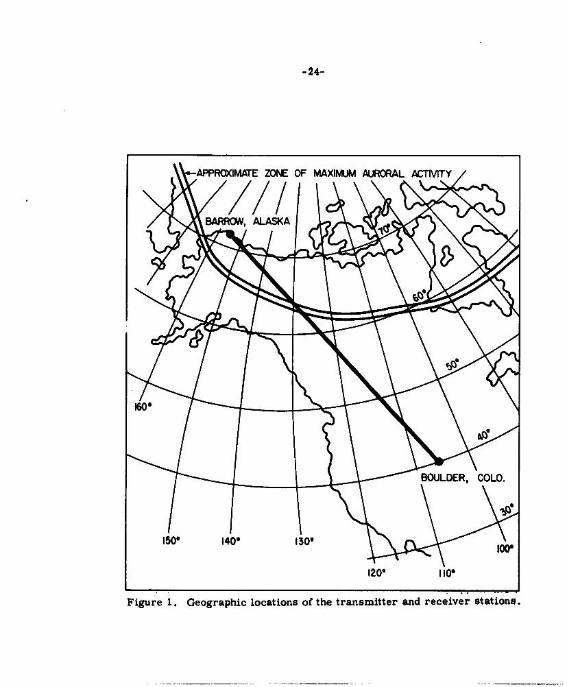
All of the measurements were made on the 4470-km transauroral

path from Barrow, Alaska,to Boulder, Colorado,at carrier frequencies

of 14. 688 Mc/s and 19. 247 Mc /s. Figure 1 shows the location of the

path relative to the auroral zone. This is typically a two-hop path for

the frequencies used, although on occasion electron densities may be

high enough to support three -hop propagation. One -hop propagation

of the Pederson ray is also possible, but it is usually much lower in

amplitude than the dominant two-hop mode, so its effect on the measure-

ments is probably insignificant.

-3-

2. EXPERIMENTAL FACILITIES COMMON TO BOTH EXPERIMENTS

The transmitters were located at the Arctic Research Laboratories

Camp at Barrow, Alaska, and were operated at a nominal 2-kw output.

Carrier frequency stability was maintained at about one part in

108 by high-quality crystal oscillators. The transmitting antennas

were quarter-wave monopoles.

The receiving facilities were located at the National Bureau of

Standards Table Mesa Field Site, approximately ten miles north of

Boulder, Colorado. The receiving antenna was either a half-wave

dipole, one wavelength above ground, or a Signal Corps Type A

rhombic antenna. All antennas were oriented on the great-circle path

to Barrow.

High-quality communication receivers were used with all receiver

oscillators crystal-controlled and having stabilities comparable to

those of the transmitted frequency. Triple conversion was used to

obtain a 10-kc/s IF which was available for recording on magnetic

tape or other processing (see figure 2).

Continuous strip chart records of field strength and fading rate

were also made in order to facilitate later data analysis. The receiving

and recording equipment was essentially the same as that used previously

by others at NBS [Koch and Petrie, 1962; Koch and Beery, 19621.

3. FADING CORRELATION BANDWIDTH

Fading correlation bandwidth is defined as the frequency spacing

at which the normalized correlation coefficient of the envelopes of two

cw carriers falls to 0. 5. In this experiment correlation bandwidth

was measured by plotting a curve of envelope correlation versus

frequency spacing.

-4-

In the transmission of analog information it is usually desired to

have a flat frequency response over the band occupied by the signal.

The fading correlation bandwidth is a measure of how well this is

achieved. In some systems diversity reception is used to obtain

improved performance. The improvement is not significant unless

the correlation between channels is on the order of 0.6 or less [ Staras,

1956] . The fading correlation bandwidth would be indicative of the

frequency spacing needed in a frequency diversity scheme.

Fading of an HF carrier is due to two principal causes, slow

fading due to changes in absorption and faster fading due to interfer-

ence among the multipath components. The absorption will affect all

frequencies within normal HF communication bandwidths in a similar

manner, whereas the multipath interference will result in fading which,

in general, will not occur simultaneously over the frequency band of

interest. This effect is called selective fading and is the heart of the

fading correlation bandwidth problem.

3.1. A Theoretical Model

No complete theoretical analysis of the fading correlation problem

has come to the author's attention although estimates have been made

based on a simplified model [Staras, 1958 ]. If one assumes that the

received signal contains two phase-coherent multipath components

with a path- length difference corresponding to D seconds and a frequency

such that the differene. corresponds to a multiple wavelength, the two

components will add in phase. At other frequencies, such that D

corresponds to an odd multiple of a half-wavelength, the two signals

will arrive out of phase and cancel. Thus minima and maxima occur

alternately as the frequency is varied, the spacing between adjacent

-5-

minima and maxima being - and from maxima to maxima or minima1 2D

to minima being -F-. The frequencies at which maxima and minima

occur are assumed to vary due to slight changes in the differential time

delay, resulting in fading at any particular frequency as the maxima

and minima move past. In the case of HF propagation, this is assumed

to be caused by changes in the ionosphere.

Over bandwidths that are small compared to the reciprocal of

the delay difference, fading will be well correlated. At frequency1

spacings on the order of -- , i.e., the maxima to minima spacing, one

would expect negative correlation. The correlated bandwidth would1

then be somewhat less than -. Using this simplified model, one would2D 1

also expect good correlation at frequency spacings of multiples of -1

and poor correlation at odd multiples of --. Then the correlation as

a function of frequency spacing would have an oscillatory component

of period 1D"

An HF communication channel is frequently more complicated

than the model just described. The multipath components do not, in

general, traverse exactly the same portions of the ionosphere and,

therefore, are affected independently by the smaller ionospheric

perturbations. This introduces a randomness which obscures the

well-defined multipath components of the model. Scatter propagation

would be an extreme example of this, since in the scatter mode there

are many multipath components and a continuum of multipath delays.

This would destroy any periodicity in the correlation function, and one

would expect the correlation to be a monotonically decreasing function

of frequency spacing, eventually vanishing for sufficiently wide spacings.

This is indicated in the brief measurements made by Koch [1958] on

ionospheric scatter propagation. Then, for HF propagation, one would

-6-

expect the fading correlation coefficient to decrease with increasing

frequency spacing with, perhaps, a periodic component, depending

upon the number and coherence of the multipath components. The

periodic portion of the correlation would be expected to decay at

increased spacings. The fading correlation bandwidth would be

inversely proportional to the multipath delay.

3.2. Experimental Results

The CW carriers at appropriate frequency spacings were obtained

by modulating the AM transmitters at Barrow, Alaska with an audio

tone. This yielded an output consisting of a 2-kw carrier and 360-watt

sidebands displaced above and below the carrier by the audio tone.

The modulation level was maintained at 85%. By using the carrier

and a sideband or the two sidebands one could determine correlations

for two frequency spacings simultaneously, i. e., spacings equal to the

audio tone and twice the audio tone. Although it would have been

desirable to have several frequency spacings available simultaneously,

logistics and signal-to-noise ratio considerations prevented it.

The received signal was translated to a 10-kc/s IF and recorded

on magnetic tape for later analysis. No receiver AGC was used. The

recorded IF signals were played back through narrow bandpass filters

which selected two components of the transmitted spectrum. Diode

detectors extracted the envelope amplitudes which were then correlated

(see figure 3). The correlation circuitry and procedure are described

in the Appendix.

It is possible to obtain two estimates of the correlation coefficient

simultaneously at the same frequency spacing by correlating the upper

and lower sidebands with the carrier.

-7-

In comparing these simultaneous sideband carrier measurements

approximately three-fourths differed by less than 20% or an absolute

difference of less than 0. 1. The data showed no preference for which

sideband would produce the greater correlation with the carrier, and

for analysis the two measurements were averaged.

A total of 56 observations was made and analyzed, 43 on 19 Mc/s

and 13 on 14 Mc/s. In all but three cases the rhombic receiving

antenna was used to obtain improved signal-to-noise ratios and reduce

off-path interference. Observations were made on January 27 and 31,

February 1, 2, 3, and 7, 196Lon 19 Mc/s and on February 17 and

24, 196Lon 14 Mc Is. Observations ranged from 3 to 15 minutes in

duration and were made between the hours of 1130 and 1845 MST

(105° West Time).

Figure 4 is a mass plot of all the data that were obtained. The

simultaneous estimates of the correlation coefficient for frequency

spacings of one and two times the modulating tone are joined together

by a straight line. The modulating tone was varied on a prearranged

schedule from 0. 2 to 3.0 kc/swhich resulted in spacings from 0.2

to 6.0 kc/s. Unfortunately a very limited amount of data was obtained

at the lowest frequency spacing.

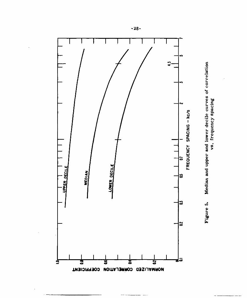
It is readily apparent that the fading correlation bandwidth can vary

appreciably. Median and upper and lower decile correlation curves

based on figure 4 are shown in figure 5. The correlation bandwidth

(correlation a 0. 5) for the median curve is about 4 kc/s,while the value

exceeded 90% of the time is 1 kc/s. It appears that the 10% value was

considerably more than 6 kc/s.

-8-

The wide variation in bandwidth was investigated by subdividing

the data according to different parameters. Parameters used were

fading rate, time of day, magnetic activity, and the ratio of the operat-

ing frequency to the MUF. The subdivision could not be carried too

far because of the limited amount of data. Although the effects of these

parameters were examined separately, they are related. The MUF

varies with time of day and is affected by magnetic activity while

fading rate is a complex function of many factors.

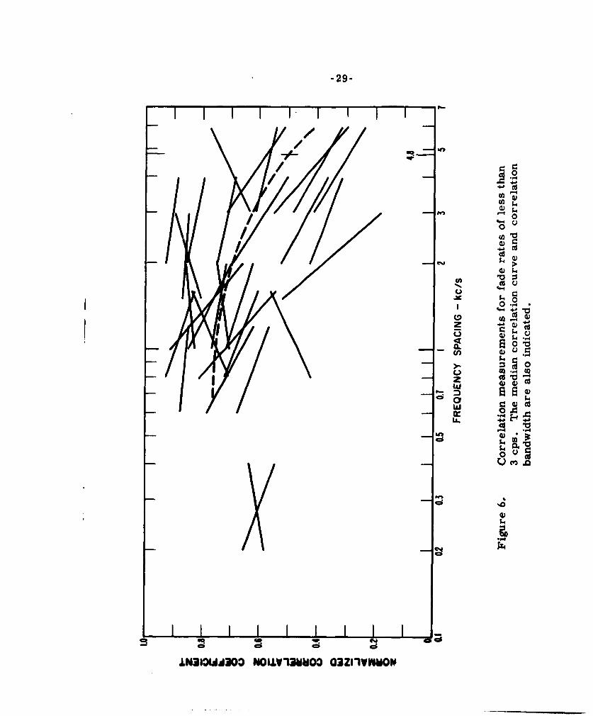
To study the effectb of fading the data were subdivided into groups

of fast and slow fading, with 3 fades per second as the dividing line.

Smaller subdivisions were tried but did not seem to yield any more

information. As shown in figures 6 and 7 the median fading correlation

bandwidth for fading rates of less than 3 c/s was 5 kc/s, while for

fading rates greater than 3 c/s it was 3 kc/s. This indicates a possible

dependence upon fading rate. Previous experience on this path had been

that low fading rates are usually associated with magnetically quiet

days and signals which frequently have periodic fading, indicating only

two dominant coherent multipath components, while higher fading rates

are usually associated with disturbed days and a more random type of

fading, indicating the presence of scattering or turbulence in the

ionosphere.

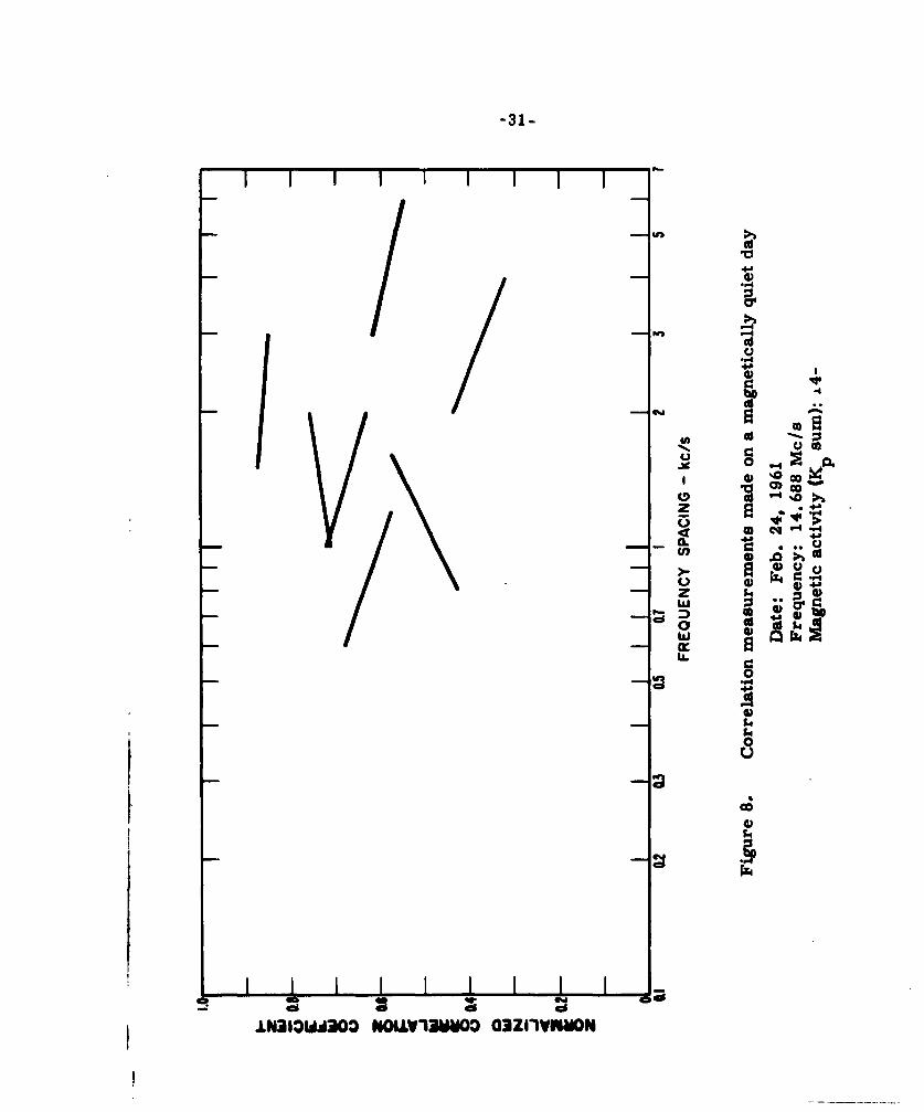
The difference between quiet and disturbed days can be seen by

referring to figures 8 and 9. Figure 8 is for a quiet day with fading

rates of less than 1 c/s during all the observations, while figure 9

is for a magnetically disturbed day with fading rates for all observations

of about 7 or 8 c/s. Both sets of observations were at 14 McIs, the

quiet-day observations being made between 1515 and 1845 MST and

the disturbed-day observations between 1145 and 1500 MST, which

in each case was the time of day providing the best signals. The

-9-

quiet-day signals were 15 to 20 db stronger than the disturbed signals.

A comparison of MUF's for the two days was impossible because

excessive absorption on the northern half of the path prevented foF2

observations. Although there is hardly enough data in either case to

draw a meaningful median curve, it is apparent that the bandwidth was

greater on the quiet day.

The data were also examined for effects related to the time of day.

Figure 10 contains median curves of correlation versus frequency spacing

for various times of the day. Three of the periods are of one-hour

duration while the earliest and latest were made somewhat longer in

order to maintain about the same number of samples in each group.

The median curves suffer from a degree of inaccuracy because of the

limited data in each group,but they do indicate a trend. The fading

correlation bandwidths have been tabulated in table 1. There appears

to be a broad minimum about 1400 MST which corresponds to about

1300 at the path midpoint. This is not unexpected since at that time

of day the MUF would be highest, resulting in greater multipath delay

for fixed-frequency operation.

Table 1.

COMPARISON OF FADING CORRELATIONBANDWIDTH WITH TIME OF DAY

Time of Day Bandwidth

1100-1300 MST 4.75 kc/s

1300-1400 2.8 kc/s

1400-1500 2.8 kc/s

1500-1600 5.9 kc/s

1600-1845 MST 5.5 kc/s

-10-

It was intended to examine the effect of the ratio of operating

frequency to the two-hop MUF, but insufficient information was avail-

able for a reasonable analysis. The MUF was to be determined by

extrapolating the foF2 critical frequencies obtained from vertical

soundings at Fairbanks, Alaska, and Boulder, Colorado, to the path

reflection points and then applying the secant + factor for oblique

incidence. Excessive absorption and sporadic E on the northern half

of the path prevented determination of MUF's on all but quiet afternoons.

Figure 11 contains all of the observations for which the MUF was

determined. The number associated with each line is the ratio of

operating frequency to the MUF. The median ratio was 0.87 which,

using Salaman's [1962] MRF curves, indicates multipath differential

delays on the order of 0.5 msec. Since the data included in figure 11

were obtained under conditions in which the multipath components

would be well-defined, there should be a minimum in the correlation

near 1 kc/s and a maximum near 2 kcls. Although there is not much

evidence of the minimum, mostly due to a lack of data, there is some

indication of a maximum near 2 kc/s. The highest values of correlation

appear in the proper area, and also the data segments with positive slope

in the 1 -kc/s to 2-kc/s area contribute to the appearance of a maximum

near 2 kc/s. This corresponds to a plausible high-low ray multipath

difference of about 0. 5 msec.

About 20% of the observations resulted in data segments having

a positive slope, with the great majority occurring on relatively quiet

days (see figure 4). This is further support of the theoretical model

described earlier.

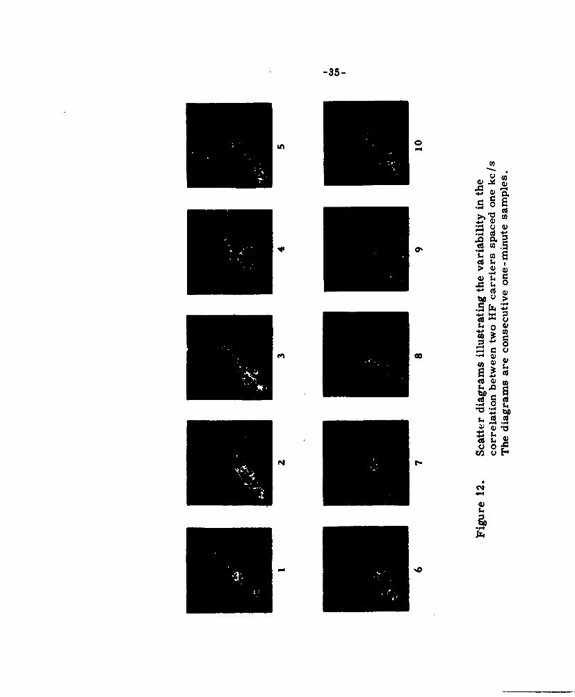
In considering these results it is well to keep in mind that the

correlation coefficients were obtained by averaging over periods rang-

ing, in all but one case, from 5 to 15 minutes. The minute-to-minute

-11-

variations can be quite large. Figure 12 contains a series of scatter

diagrams made at one-minute intervals. The diagrams were made in

the conventional manner by applying the envelope voltage of the upper

sideband to the vertical deflection plates of an oscilloscope and the

carrier envelope to the horizontal deflection plates. The frequency

spacing between the two signals was one kc/s. The diagrams represent

one-minute samples and were made consecutively. One could estimate

the correlation directly from these diagrams (Sugar, 1954], but they

were included here only to show how the correlation can change from

minute to minute.

4. SHORT-TERM FREQUENCY PERTURBATIONS OF AHIGH-FREQUENCY CARRIER

Although modern technology has achieved very accurate control of

the carrier frequency of HF transmitters, there are usually uncontrolled

frequency variations in the received signal due to the vagaries of

ionospheric propagation. These variations can be divided into long-term

changes, i.e., durations of minutes or hours, due to diurnal changes

in layer heights or electron densities and short-term changes, i.e.,

on the order of milliseconds, due to interference among the various

multipath components.

Investigations of long-term changes [ Fenwick and Villard, 1960;

Watts and Davies, 1960] have shown frequency shifts as great as 5 or

6 cps. Such variations would be important in applications such as

monitoring of standard broadcasts but probably would be inconsequential

in FSK digital communications. The much larger short-term changes

which would be important in communication system performance have

been, for the most part, neglected. These changes are the subject of

this part of the report.

-12-

4. 1. Theoretical Curves

The variation in instantaneous frequency that results frnm the

interference between two unmodulated carriers of approximately the

same frequency has been described many times. Curves similar to

those obtained by Cuccia [ 1952] which illustrate the variations of

instantaneous frequency for several amplitude ratios of the interfering

carriers are shown in figure 13.

One might use this description as the basis for a model of the HF

signal, but it would be of limited value. Although the received signal

may frequently contain only two multipath components and, therefore,

fit the preceding description, the amplitude ratio will vary widely as

the two components fade independently. The frequency difference will

also be subject to random variations. As a result the model chosen

for comparison with the observations should be of a random nature.

This would be especially true when the received signal contains many

multipath components.

In view of this and the fact that the amplitude statistics of an HF

signal are frequently approximated by Rayleigh distributions, a model

based on narrow-band Gaussian noise seems appropriate. Some

statistics for the instantaneous frequency of such a model have already

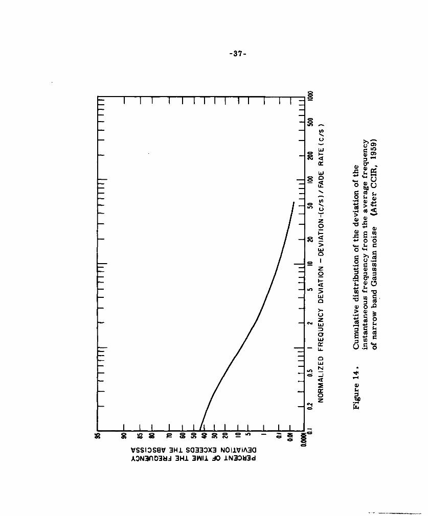
been obtained [ CCIR, 1959] . In this case, for simplicity, a rectangular

noise spectrum was assumed, although a Gaussian-shaped spectrum

would probably be a more accurate representation. The theoretical

distribution of deviations from the average frequency are given in

figure 14. The frequency deviation has been normalized with reference

to the fading rate, the fading rate being 1/2.32 times the width of the

rectangular noise spectrum.

-13-

Cumulative distributions alone are not sufficiently revealing;

information is also needed about the duration of the frequency excursions.

Theoretical distributions containing this information are not available,

but measured distributions were obtained. The aforementioned CCIR

report does give average duration of the frequency excursions as a

function of frequency deviation.

4. 2. Experimental Results

Observations of the instantaneous carrier frequency were made

over the same path and with the same transmitting and receiving

equipment as the correlation measurements (see figure 2). Data were

obtained on both 14. 688 Mc/s and 19.247 Mc/s from August 9, 1961

to August 22, 1961, using both dipole and rhombic receiving antennas.

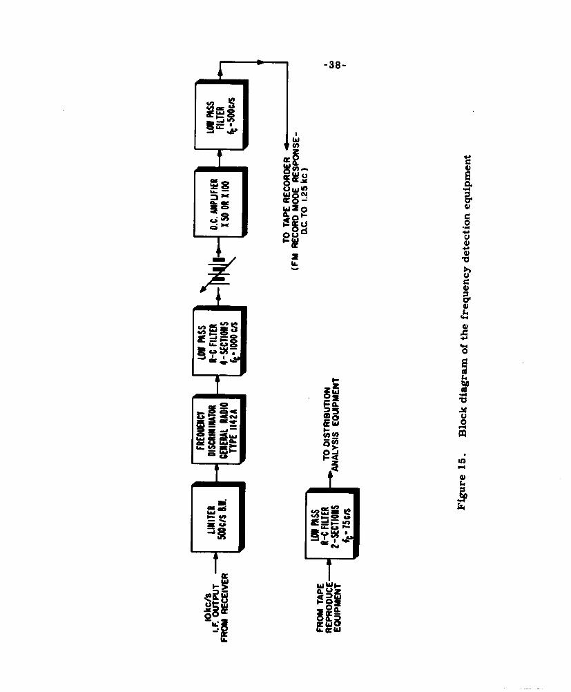
Figure 15 is a block diagram of the frequency-detection equipment.

The 10-kc/s IF signal from the receiver was amplitude-limited and then

fed to a frequency discriminator. The discriminator produced a pulse

of constant amplitude and width with the leading edge coincident with

the positive-going zero-crossings of the input signal. The result was

pulse train whose average d-c level was proportional to the input

frequency. In this situation the 10-kc/s and higher frequency components

arising from the pulse repetition rate were removed by filtering, leaving

approximately 10 volts d-c corresponding to the 10-kc/s input frequency.

The average d-c level was subtracted by the series d-c supply, leaving

voltage variations corresponding to the frequency deviations from the

average carrier frequency. At the output of the discriminator the scale

factor was 1 mv/cycle.

-14-

Equipment noise was sufficiently low to permit observation of

frequency changes of less than one c/s. Unfortunately this was not

always true when actual signals were being observed, the received

signal-to-noise ratio frequently being such as to mask the smaller

frequency changes. In addition, the large frequency changes were

usually accompanied by fading of the carrier which resulted in addition-

al noise degradation of the signal. To alleviate this condition during

data reduction, the post-detection bandwidth was redAced to 75 c/s by

adding a low-pass filter between the tape-playback equipment and the

analysis equipment. Figure 16a illustrates the improvement obtained

by addition of the filter. The cut-off frequency chosen did not seem to

have a serious effect on the desired data. This bandwidth was also

comparable to the post-detection bandwidth in single-channel FSK

systems. Figure 16b depicts some of the frequency perturbations that

were observed. Note that the frequency changes appear in both direc-

tions and are coincident with fades in envelope amplitude. This was

typical of signals with low fade rates, and was similar to the situation

of two interfering carriers described earlier (figure 13). Figure 16c

illustrates the more random variations found at higher fade rates.

The equipment used for data reduction was essentially the same

as that used previously for analysis of fading on this path [Koch, Beery,

and Petrie, 1960] . Cumulative distributions of frequency deviation

from the average frequency were obtained as were distributions of

frequency deviation exceeded for various durations from 1.0 to 100 or

250 milliseconds.

-15-

All distributions were based on a 200-second sample length. The

curves are presented as averages of the deviation on each side of the

carrier. This results in the distribution being asymptotic to the 50%

line as the deviation approaches zero.

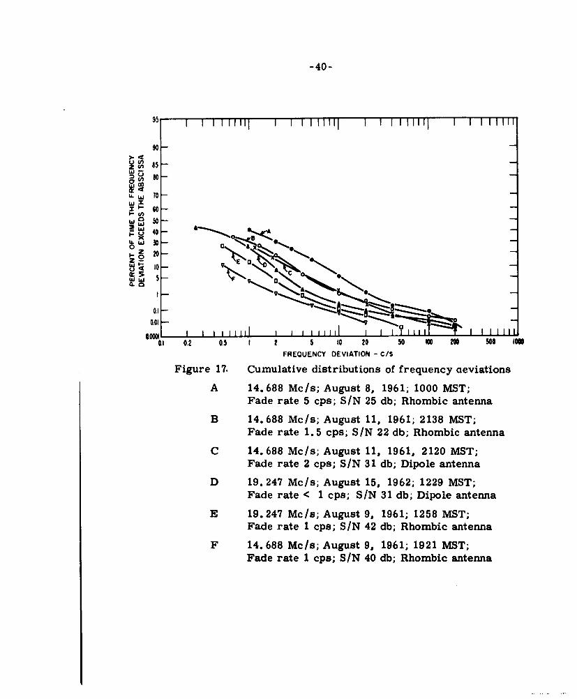
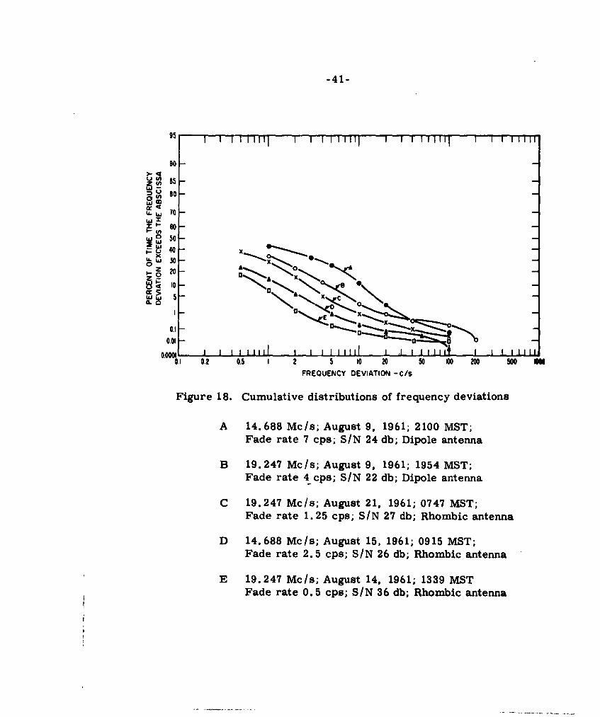
The cumulative distributions followed the general shape of the

theoretical curve. Examples for a variety of fade rates are given in

figures 17, 18, and 19. A comparison with the narrow-band noise

model was made by translating the measured curves to the left or right

to bring them into coincidence with the theoretical curve. Because of

the logarithmic frequency scale, this was equivalent to dividing the

frequency excursions indicated by the curve by a normalizing factor.

Obviously,exact coincidence is not obtained unless the curves have

identical shapes. The agreement between curve shapes ranged from"good" to "poor" as shown in figure 20. If, because of curve shape,

there was some question as to the exact normalizing factor, coincidence

of the right-hand portions of the curves was weighted most heavily,

since this is the area of interest from the standpoint of FSK telegraph

errors.

The normalizing factor obtained in this manner is plotted versus fade

rate in figure 21. A straight line having a reasonable fit to these points

has a slope of 1.4. This is to say, on the average, frequency deviations

occurred with probabilities given by the theoretical curve, if 1.4 times

the fade rate is used in place of the fade rate for the normalizing factor.

It should be realized that this factor was obtained from a limited

number of observations on a particular path and may be different for

other situations.

-16-

A factor closer to unity might have been obtained if the model had

used a Gaussian-shaped noise spectrum instead of a rectangular-shaped

spectrum. The long "tails" on the Gaussian-shaped spectrum would

have contributed to more violent frequency excursions and might have

made the theoretical distribution more directly comparable to the

observed distributions.

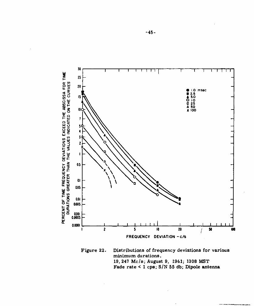
Cumulative distributions of frequency deviation do not give any

insight into the duration of individual frequency excursions. For this

type of information one is referred to figures 22 through 29. These

figures are families of curves giving the per cent of time that the

frequency excursions exceed a given magnitude for periods greater

than a given duration. Each figure contains a family of curves obtained

from the same data sample with duration as the parameter. The figures

given are typical of the data that were obtained. Figure 23 illustrates

the smallest frequency deviations observedwhile the largest deviations

are given by figure 29 for durations up to 25 msec and by figures 27 and

28 for durations of 50 and 100 msec respectively.

Unfortunately, similar distributions are not available for the

theoretical model. The CCIR report mentioned earlier does contain

curves of the average duration of frequency deviations exceeding

particular values. The data reduction methods used did not permit

comparison with this information.

5. CONCLUSIONS

Measurements of the correlation. between the fading envelopes of

HF carriers at frequency spacings from 0.2 to 6.0 kc/s indicated a

mean fading correlation bandwidth of 4.3 kc Is. The bandwidth that

was exceeded 90% of the time was 1.0 kcls. The upper decile value

was not obtained because it exceeded the largest spacings observed.

-17-

The effect of fading rate and magnetic activity was investigated.

The fading correlation bandwidth was found to decrease with increased

magnetic activity and with increased fade rate.

The effect of time of day was also investigated,and a broad

minimum in correlation bandwidth was found about midday. This

minimum coincides with the minimum in the ratio of the observed

carrier frequency to the lowest order (two-hop) MUF. At this time

high-low ray differential multipath delays would be the greatest,

indicating a general agreement with what was suggested by the rather

elementary model described earlier, i.e., that the fading correlation

bandwidth is inversely proportional to the multipath delay.

A lack of detailed propagation information prevented a more

detailed examination of the relationship between correlation bandwidth

and the ratio of the operating frequency to the MUF. There is some

evidence, however, that the correlation versus frequency spacing function

contains an oscillatory component whose period is the reciprical of the

delay time, as was suggested by the simplified model.

It is suggested that future correlation measurements be made

concurrently at several frequency spacings to provide more detailed

information as to the nature of the correlation versus frequency spacing

function. Simultaneous sweep-frequency pulse transmissions over the

same path would be invaluable in determining what propagation modes

were present, and would allow one to relate the bandwidth measurements

to the propagation characteristics. Such information would permit some

degree of prediction of bandwidth in the future, on the same or other

paths.

-18-

Statistical distributions were obtained of the frequency deviation

of an HF signal from its average carrier frequency. These distri-

butions were compared with a theoretical distribution based on a narrow-

band noise model. Reasonable agreement was obtained if a normalizing

factor of 1.4 times the fade rate was used rather than the fade rate.

Distributions were also obtained which indicate the duration of the

frequency deviations. These were not compared with theoretical

distributions. The results do indicate that frequency deviations of this

nature would not be a significant source of errors in FSK digital com-

munications for the frequency shifts and baud rates commonly used,

i.e., for shifts of greater than 100 c/s, and element lengths greater

than 10 or 15 msec.

Because frequency deviations were found to be closely related to

fading rate and only indirectly to other propagation parameters, and

because of the difficulty of precise mode determination without simul-

taneous sweep frequency recordings, comparisons of frequency devia-

tions with factors other than fade rate were not attempted.

6. ACKNOWLEDGEMENTS

The logistical support and other assistance provided by the Arctic

Research Laboratory, Barrow, Alaska, Max Brewer, Director, was

invaluable and greatly appreciated.

The author also appreciates the assistance of J. L. Workman

(Barrow, Alaska), G. E. Wasson, E. L. Komarek, and C. H. Johnson

in obtaining and analyzing the data and the advice and comments of

R. K. Salaman on propagation problems. The author also acknowledges

the work of J. W. Koch in originating the project.

i

-19-

7. REFERENCES

Bell, J., Correlation between fading signals, Electronic Technology

23, 36-40 (Jan. 1960).

C. C. I. R., Influence on long-distance high-frequency communications

using frequency shift keying of frequency changes due to passage

through the ionosphere, Report No. 111, IXth Plenary Assembly,

Los Angeles 3, 89 (1959).

Cuccia, C. L., Harmonics, sidebands and transients in communication

engineering, 287-289 (McGraw Hill, New York, N.Y., 1952).

Davenport, W. B., Jr., R. A. Johnson, and D. Middleton, Statistical

errors in measu:rements on random time functions, J. Appl. Physics

23, 377-388 (April 1952).

Fenwick, R. C., and 0. G. Villard Jr., Continuous recordings of the

frequency variation of the WWV-20 signal after propagation over

a 4000 km path, J. Geophys. Research 65, 3249-3260 (Oct. 1960).

Koch, J. W., Factors affecting modulation techniques for VHF scatter

systems, IRE Trans. of PGCS CS-7, 77-92 (June 1959).

Koch, J. W., and H. E. Petrie, Fading characteristics observed on

a high-frequency auroral radio path, NBS Jour. of Res. 66D,

159-166 (Mar. - Apr. 1962).

Koch, J. W., and W. M. Beery, Observations of radio wave phase

characteristics on a high-frequency auroral path, NBS Jour. of

Res. 66D, 291-296 (May-June 1962).

Meyers, K. A., and H. B. Davis, Triangular-wave analog multiplier,

Electronics 29, 182-186 (August 1956).

Norsworthy, K. H., A simple electronic multiplier, Electronic

Engineering 26, 72-76 (Feb. 1954).

-20-

Salaman, R. K., A new ionospheric multipath reduction factor

(MRF) IRE Trans. of PGCS CS-10, 220-222 (June 1962).

Staras, H., Diversity reception with correlated signals, J. Appl.

Physics 27, 93-94 (Jan. 1956).

Staras, H., Tropospheric scatter propagation - a summary of recent

progress, RCA Review 19, 3-18 (March 1958).

Sugar, G. R., Estimation of correlation coefficients from scatter

diagrams, J. Appl. Physics 25, 354-357 (March 1954).

Watts, J. M., and K. Davies, Rapid frequency analysis of fading

radio signals, J. Geophys. Research 65, 2295-2303 (August 1960).

-21-

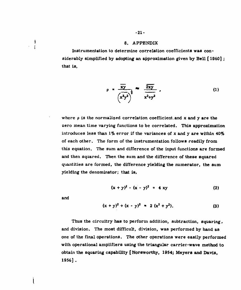
8. APPENDIX

Instrumentation to determine correlation coefficients was con-

siderably simplified by adopting an approximation given by Bell [ 1960];

that is,

(x2y2)* x2+y

where p is the normalized correlation coefficient.and x and y are the

zero mean time varying functions to be correlated. This approximation

introduces less than 1% error if the variances of x and y are within 40%

of each other. The form of the instrumentation follows readily from

this equation. The sum and difference of the input functions are formed

and then squared. Then the sum and the difference of these squared

quantities are formed, the difference yielding the numerator, the sum

yielding the denominator; that is,

(x+y)2 - (x-y) 2 = 4xy (2)

and

(x+y)2 +(x- y)2 a 2 (x 2 +y 2 ). (3)

Thus the circuitry has to perform addition, subtraction, squaring,

and division. The most difficult, division, was performed by hand as

one of the final operations. The other operations were easily performed

with operational amplifiers using the triangular carrier-wave method to

obtain the squaring capability [Norsworthy, 1954; Meyers and Davis,

1956].

-22-

The square-law characteristic is due to the area of similar triangles

being proportional to the square of their heights. If a triangular wave

of zero mean and peak amplitude V is full-wave rectified, the average

value is IV. If to the triangular wave is added a signal s, which varies

slowly compared to the triangular wave frequency, the average rectified

output will be 2(V + s2).

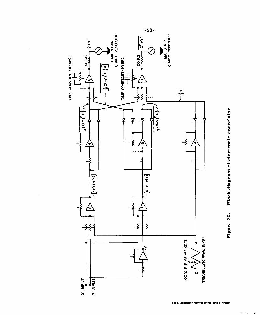
Figure 30 is a diagram of the correlator. The triangular blocks

represent operational amplifiers, while the numbers adjacent to the

input and feedback resistors indicate relative values. Amplifier 1

provides a sign reversal for the Y input,while amplifiers 2 and 3 are

adders to form the sum and difference of the two inputs. Amplifiers

4, 5,and 8 are phase inverters to drive the full-wave diode rectifiers.

Germanium diodes were used because of their low forward voltage

drop. The only other requirement on the diodes is a sufficiently high

inverse voltage rating, since peak voltages were as high as 100 V.

Amplifiers 6 and 7 are combined adders and integrators, integrating

with a 10-second time constant.

In unit 6, the squared terms and the constant due to the triangular

carrier wave cancel, leaving the cross product average, while in unit

7 the cross products cancel, leaving the sum of the squares in the

output, the carrier-wave constant being removed by adding in a similar

constant of proper sign from amplifier 8.

One percent resistors were used for input and feedback elements.

Some minor gain adjustments were made at the input to the integrator

units to assure cancellation of the undesired input terms.

The outputs of units 6 and 7 were recorded on strip charts, one-

minute averages taken, and the quotients formed manually. This

resulted in a curve of correlation coefficient versus time, which was again

averaged to obtain a single value for each run.

-23-

By definition the correlation coefficient implies averaging over

infinite time. 'The loss of accuracy due to finite averaging time has

been discussed at length elsewhere [Davenport, Johnson, and

Middleton, 1952].

Multiple averaging as performed here is a method of avoiding

some of the errors due to finite averaging time. Bell [1960] indicates

that for applications such as this the observation period should be at

least 100 times the interval between fades in order to obtain results

significant at the 95% level for correlation coefficients on the order of

0.2. The observation times used in this experiment more than met

this criterion.

This instrumentation scheme assumes that the input signals have

zero means. This was accomplished by using long time constant RC

coupling circuits. To eliminatt the error that would be introduced by

the charging of the coupling capacitors at the beginning of a run,

provision was made for shorting out a large portion of the coupling

circuit resistance in order to rapidly charge the coupling capacitor to

approximately the mean value. An alternative was to make a pre-

liminary run to charge the coupling capacitors and then play back the

data again to obtain the correlation coefficient. This was especially

useful on short runs where one could not afford to discard the initial

portion of the run.

-24-

APPROXIMATE ZONE OF MAXIMUM AURORAL ACTIMTY

BARRON, ALASKA

S• BOULDER, \COLO.

150 140 100"

1200 1100

Figure 1. Geographic locations of the transmitter and receiver stations.

-25-

cc U cm=" L&.

dc~

- 0

0c= C= c

C.. La. %- 94 G

L" s

Zo . 1

C; __o_ _a_ _W_

cmU3U,~~C~ __ _ _3___ _ __ _ _+_ _

-26-

LI -AIae Co

P.-

°fl

0'

LLAJ LAJ a)L f

-. o

_ $4

U w

=• cU

0

ca $4

Lai

CL.-

110

-27-

05.4

Cc0

w0IAU.

$4

ci0

co4

IN31DUA300~~ 0OI'3NDC)Z-V4O

-28-

04

0ý4-

-j U.

a 0~

.- 4

Ilk

CD,

IN31L"30 NOLVI1MMD 03IIV4Vz

-29-

.4)

.3c 0

00

~0o

CS

LL

Z -4

IN

JN3I0WAIDOO NOLLV13VOO a3ZivW~ONo

-30-

II. I I I I I 4It

/>

/ CL

/z/w/w

4-14

/ 540

IcIN31OW4300 ~ ~ ~ ~ N0VUO 13IV&

Co.

-44

4a

CYw~

ac U

INBOOMAD0 Novim 'azilw"r

-32-

-4 -44 +

C. cl

JLN31WA30 NOII13vw 03Z fMMO

-33-

IIL

0

-%j

00

0~0z . .

w , 0U

w0 cr z

o f

0

8S4L.4

±N3I01d43O0 NOlIV13MOOO 03ZIIVWWON

-34-

44

J .500

44

$4 C

00

IVL

o~

5T4O

'o %.W

cin

0)1DA0 NI-MNO03I~4O

-35-

00

Ci20co

td M

02S,

4 -

Q402

4)5

.r4o

-36-

X-0.9"

-X.1.0

5

WI -WA 4%-4e

X8.o

X.O.2-

I 5

4(Cjk-we) t

Figure 13. Deviation of the instantaneous frequency (w.) about thestronger (cA) of the two interfering carriers (w A and w B)

The deviation is given in units of the frequency differencebetween the two carriers for various values of the ratio(x) of the amplitudes of the carriers. (after Cuccia)

-37-

Lr)

C20

04.)

z GG

0 0

40 0Uo - 4C

w 0 O4-4

414

otz0

~~tLJ _g4. 4

wW

LL.i

VSSIDSSV 3HI S0330X3 NOILVIA30ADON3nO38. 3HI 3VNII1 JO IN30k3d

-38-

_w 0.

0 Atuw4I

-0 0

C)

:)5)

w 0

I-

Fam

090

44

0.

-39-

(a)

(b)

(c)

Figure 16. Illustrations of observed frequency deviations

(a) Effect of 75 cps low-pass filter on outputUpper trace - with filter; Lower trace - without filterTime base 0.2 sec/div. ; Vertical scale 20 cps/div.

(b) Frequency deviation (upper trace) and envelope voltage(lower trace) for an average fade rate of 1 cpsTime base 0. 2 sec/div. ; Vertical scale 20 cps/div.Envelope voltage uncalibrated

(c) Frequency deviation (upper trace) and envelope voltage(lower trace) for an average fade rate of 4 cpsTime base 0.25 sec/div.; Vertical scale 20 cps/div.Envelope voltage uncalibrated

-40-

95

90-

Zc 85-

WO030

I-,, )'

00, -2

z 2D

Uj85 - l~

0.1 l

11 0.2 0.5 I 2 5 10 20 50 0 M 500 Im

FREQUENCY DEVIATION - C/S

Figure 17. Cumulative distributions of frequency aeviations

A 14.688 Mc/s; August 8, 1961; 1000 MST;Fade rate 5 cps; SIN 25 db; Rhombic antenna

B 14.688 Mc/s; August 11, 1961; 2138 MST;Fade rate 1.5 cps; S/N 22 db; Rhombic antenna

C 14.688 Mc/s; August 11, 1961, 2120 MST;Fade rate 2 cps; S/N 31 db; Dipole antenna

D 19. 247 Mc/s; August 15, 1962; 1229 MST;Fade rate < 1 cps; S/N 31 db; Dipole antenna

E 19. 247 Mc/s; August 9, 1961; 1258 MST;Fade rate 1 cps; S/N 42 db; Rhombic antenna

F 14. 688 Mc/s; August 9, 1961; 1921 MST;Fade rate 1 cps; S/N 40 db; Rhombic antenna

-41-

1511II II I1 1 I lI I I I IIIII111 I I I Itl1 l

90-

,85.

U. W 10W X 60-

W0 50°w o

U 40 -I -

ojN. XN

FQEC DEIAIO -c/

Figure 18. Cumulative distributions of frequency deviations

A 14. 688 Mc/s; August 9, 1961; 2100 MST;Fade rate 7 cps; SIN 24 db; Dipole antenna

B 19.247 Mc/s; August 9, 1961; 1954 MST;Fade rate 4 cps; SIN 22 db, Dipole antenna

C 19.247 Mc/s; August 21, 1961; 0747 MST;Fade rate 1.25 cps; S/N 27 db; Rhombic antenna

D 14. 688 Mc/s; August 15, 1961; 0915 MST;Fade rate 2.5 cps; S/N 26 db; Rhombic antenna

E 19. 247 Mc/s; August 14, 1961; 1339 MSTFade rate 0.5 cps; S/N 36 db; Rhombic antenna

-42-

SI I I1Iiiit I I Il 1 i i II1 I I 111 1

90 -

z 0 85 -8 5

. ,, 70

W•-"X 60

w 5~u 40

x0U. w 3029

~ 0 EN 20 V

S,2

Au 14 688 Mcs uut1, 9192MT

0.01- -

B 19 ,i,,•, 247 c Augut 2, 1-961; 4 0 MST,,Fad 02 05 1 2 .5 c 20 52 1 , 2io antenn

FREQUENCY DEVIATION -C/S

Figure 19. Cumulative distributions of frequency deviations

A 14.688 Mc/s; August 10, 1961; 0952 MST;Fade rate 6 cps; SIN 17 db; Dipole antenna

D 19.247 Mc/s; August 21, 1961; 0737 MST;Fade rate 1.25 cps; S/N 21 db, Dipole antenna

C 14.688 Mc/s; August 16, 1961; 1040 MST;Fade rate 2 cps; S/N 22 db, Rhombic antenna

D 14.688 Mc/s; August 16, 1961; 0840 MST;Fade rate 1. 25 cps; SIN 37 db; Dipole antenna

lmE 14.688 Mc/s; August 17, 1961; 1353 MST(;Fade rate < lcps, SIN 25 db; Dipole antenna

-43-

III 1 1111 1 to

540

- J .

8 -~ *-4 tv

w

N cU v - vvUW o' >b .

0 0 0

4dN N

ci

VSSIOSSV 3Hi S0330X3 NOI.LVIA30AON3flO3UA 3HJ. 3WII1 -40 ±N33N3d

-44-

I I I

10 X

9 X

x

SLOPE 1.4

0Xu x

ZN 5 -7.0-' x

Z 4 Xx0X

IIIX

x

2 X

0 I 2 3 4 5 6 aFADE RATE, FADES PER SECOND

Figure 21. Comparison of experimentally determinednormalizing factor with the observed fadingrate

-45-

30 1 I 1 1 i I i'

25

o W 20U.> "0 1.0 msec

1 2.515Cn a 5.0

C) LLJ0 10.. • 025

MZ a. £50< z 10 I t0

W-7k

xz 4-w A

z~ = H 0

0-0:w I

w

zI.

w

I2 5 0 20 / 50 00

wp

FREQUENCY DEVIATION -C/S

Figure 22. Distributions of frequency deviations for variousminimum durations.19,247 Mc/s; August 9, 1961; 1308 MSTFade rate < 1 cps; S/N 55 db; Dipole antenna

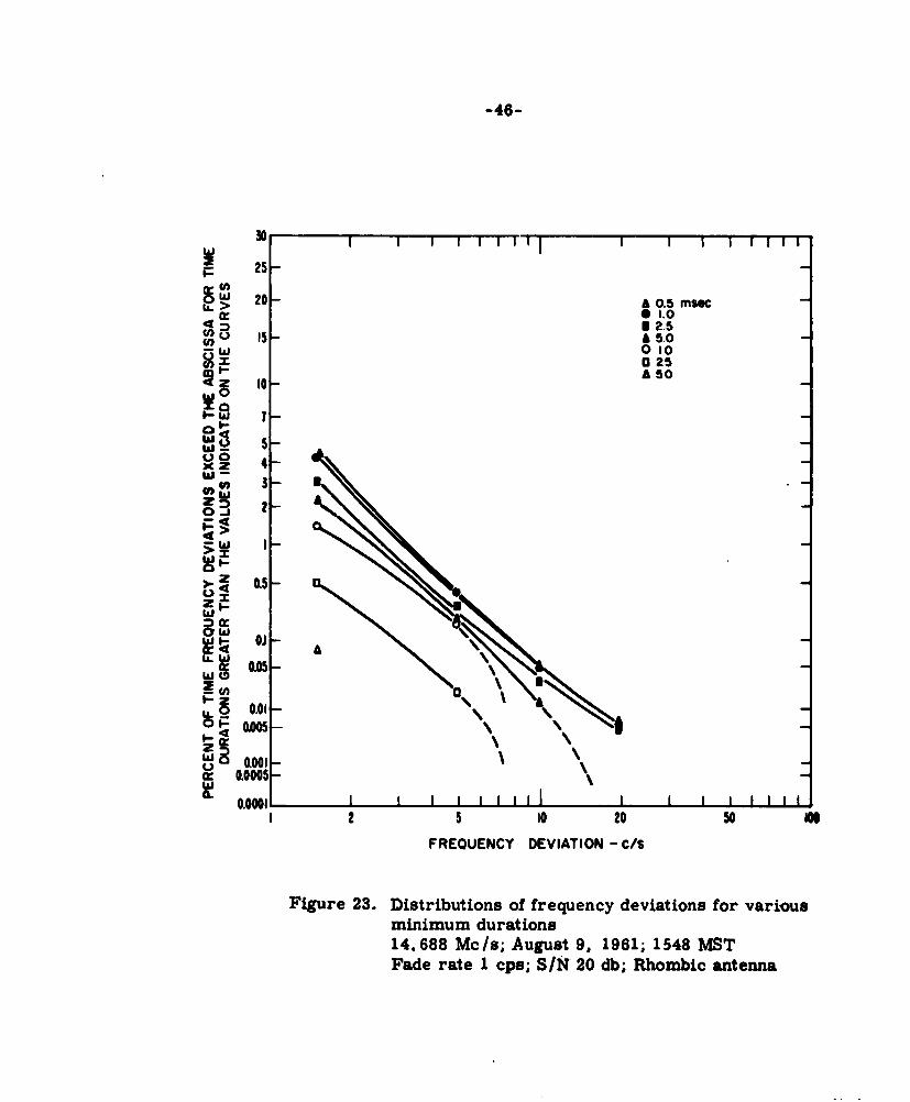
-46-

11111, I I I i ,i

25-

W' 20 a 0.5 mac01.0

-w 010x 025

IA £50

1

-W

U .xz 4-

w 3U) 2

4>X

0" OL 0.0

z I-

Ir

0.01

w O , •oo,I 0.0001

o.oo0.0001I iil I I 1111I

I 2 5 10 20 50 IN

FREQUENCY DEVIATION -C/S

Figure 23. Distributions of frequency deviations for variousminimum durations14.688 Mc/s; August 9, 1961; 1548 MSTFade rate 1 cps; S/N 20 db; Rhombic antenna

-47-

30 1 I I I I I III

25-

S01.0 msec

32.50 15 - 5.0wn 0 10

nx 0 25o £- 0 a 50

4 Z 10 - X 100, 0 0250

=0I--w T-

_ 4

wonw

z x

001P\ \

z 0.0005w

o .O.00l t l I I I II IiI I I I 1111I2 5 0 20 50 IO

FREQUENCY CEVIATION - C/S

Figure 24. Distributions of frequency deviations for va~riousminimum durations14.688 Mc/Is; August 16. 1961; 1040 MSTFade rate 2 cps; SIN 22 db; Rhombic antennaa

-48-

30 1 1I 1I I I 1

25!

0 2020. @ 1.0 msec0 2.5

15g A 5.0

w 0 10n X- 0 25Caý- A 50S- 10 x 100w 0250

w T0--w .4w Y 5

Cu-- 3

Z 'A

0 2w 0 xx

01

zU~0S0.I- 0. \ \

w "-0.005

S0 o0. -1 0.005 \\-"

• 0.0005 -

110001 I - I I I I I I I I I I I 1 -11 2 5 10 20 50

FREOUENCY DEVIATION -C/S

Figure 25. Distributions of frequency deviations for variousminimum durations14.688 Mc/s; August 15, 1961; 0915 MSTFade rate 2.5 cps; S/N 26 db; Rhombic antenna

-49-

1 130 I I I I I I

25-

"'W 20 -Cr~ 10 iom,%ec

M 2.515 U A 5.0)• o010

025a 50Sz lo- x 100

w 0

w- 4

x z 4

5 3o3 2a: £

49

>I81.-

5 o

L 0.010

w 0.051.0001 -I I I IIII I I I I I 11

1 2 5 10 20 50 100

FREQUENCY DEVIATION - C/S

Figure 26. Distributions of frequency deviations for variousminimum durations14.688 Mc/s; August 23, 1961; 0540 MSTFade rate 3 cps; S/N 19 db; Dipole antenna

-50-

30F 25-

O w 2o2-Cr 01.0 miec

3 5 2.5- 0 a 5.05w 010

025lo- a A£50

x 0

U 5 -0 4

000

w

Mw0 01 -P ,-

uw

"W S 0.05-

6 5 O 0 -o

1 -f0.05

w 0.0005

0.0001 I I I I 1 I1 J I I I 1I 2 5 10 20 50

FREQUENCY DEVIATION -C/S

Figure 27. Distributions of frequency deviations for variousminimum durations14.688 Mc/s; August 11. 1961; 2037 MSTFade rate 4 cps; SIN 30 db; Rhombic antenna

-51-

50 i I I iI F I

25-

20Wo "> 20 oL> 0 1.0 msec

D "I2.5U) s 5.003 010o

)025

z 10 - owO

w_ 5

U) 3w3 2

-

w I 0xx

z~p

oal .1o

< 0 0x

F"' \ A

0.0 \\S0.0005 - \ a

2

@001

0.005-

0.0001 I I I I I i l1 2 5 10 20 50 IN

FREQUENCY DEVIATION -c/s

Figure 28. Distributions of frequency deviations for variousminimum durations14.688 Mc/s; August 10o 1961; 1000 MSTFade rate 5 cps; S/N 25 db; Rhombic antenna

-52-

30 I I I I I1111

2 F -2

U. > 20 w. rnsec12.5

U 15 A 5.00o 10

5w 0 0 25M1-- £50

4 z lo-X 100

w• 0

wy 5-0 0

(0 3-z) D

z 2

. 0.5 -

OUJ

w ti- 0.1W{.9 Cr 0.05-

0.01o 0- 0.005-

L 0o.001 -S 0.0005-

0.00011 2 5 10 20 50 U

FREQUENCY DEVIATION - c/s

Figure 29. Distributions of frequency deviations for variousminimum durations14.688 Mc/s; August 10, 1961; 0952 MST

Fade rate 6 cps; S/N 17 db; Dipole antenna

-53-

w -~ w

Cl) 0 1 0 -

0 >1 00

Cl))

IJJt

ui

a0

>.

-4

CC.zU

ui0

z5

4.

U. 4 MMNTPRPMG "IR:IMO- U3

U. S. DEPARTMENT OF COMMERCELuther 11. Hodges, Secretary

NATIONAL BUREAU OF STANDARDSA. V. Astin, Director

THE NATIONAL BUREAU OF STANDARDS

The scope of activities of the National Bureau of Standards at its major laboratories in Washington, D.C., aidBoulder, Colorado, is suggested in the following listing of the divisions and sectionsengaged in technical work.In general, each section carries out specialized research, development, and engineering in the field indicated byits title. A brief description of the activities, and of the resultant publications, appears on the inside of thefront cover.

WASIIINGTON, D. C.

Electricity. Resistance and Reactance. Electrochemistry. Electrical Instruments. Magnetic Measurement5Dielectrics. High Voltage.Metrology. Photometry and Colorimetry. Refractometry. Photographic Research. Length. Engineering Metrology.Mass and Scale. Volumetry and Densimetry.Beat. Temperature Physics. Heat Measurements. Cryogenic Physics. Equation of State. Statistical Physics.Radiation Physics. X-ray. Radioactivity. Radiation Theory. High Energy Radiation. Radiological Equipment.Nucleonic Instrumentation. Neutron Physics.Analytical and Iorganic Chemistry. Pnre Substances. Spectrochemistry. Solution Chemistry. Standard Refer-ence Materials. Applied Analytical Research. Crystal Chemistry.Mechanics. Sound. Pressure and Vacuum. Fluid Mechanics. Engineering Mechanics. Rheology. CombustionControls.Polymers. Macromolecules: Synthesis and Structure. Polymer Chemistry. Polymer Physics. Polymer Charao.terization. Polymer Evaluation and Testing. Applied Polymer Standardsand Research. Dental Research.Metallurgy. Engineering Metallurgy. Microscopy and Diffraction. Metal Reactions. Metal Physics. Electrolysisand Metal Deposition.Inorganic Solids. Engineering Ceramics. Glass. Solid State Chemistry. Crystal Growth. Physical Properties.Crystallography.Building Research. Structural Engineering. Fire Research. Mechanical Systems. Organic Building MaterialsCodes and Safety Standards. Heat Trans'er. Inorganic Building Materials. Metallic But ding Materials.Applied Mathematics. Numerical Analysis. Computation. Statistical Engineering. MathematicalPhysics. Op.erations Research.Data Processing Systems. Components and Techniques. Computer Technology. Measurements Astoaftlos,Engineering Applications. Systems Analysis.Atomic Physics. Spectroscopy. Infrared Spectroscopy. Far Ultraviolet Physics. Solid State Physics. ElectronPhysics. Atomic Physics. Plasma Spectroscopy.Instrumentation. Engineering Electronics. Electron Devices. Electronic Instrumentation. Mechanical lamsr-ments. Basic Instrumentation.Physical Chemistry. Thermochemistry. Surface Chemistry. Organic Chemistry. Molecular Spectroscopy. El.-mentary Processes. Mass Spectrometry. Photochemistry and Radiation Chemistry.Office of Weights and Measures.

BOULDER, COLO.Cryogenic Engineering Laboratory. Cryogenic Equipment. Cryogenic Processes. Properties of Materials. Crays.genic Technical Services.

CENTRAL RADIO PROPAGATION LABORATORY

Ionosphere Research and Propagat/on. Low Frequency and Very Low Frequency Research. losomqdie Is.-search. Prediction Services. Sun-Earth Relationships. Field Engineering. Radio Warning Services. VwtUedSoundings Research.Radio Propagation Engineering. Data Reduction Instrumentation. Radio Noise. TroposphbericTropospheric Analysis. Propagation-Terrain Effects. Radlo-Meteorology. Lower Atmosphere Ph ysis.Radio Systems. Applied Electromagnetic Theory. High Frequency and Very High Frequency Researh Fr-quency Utilization. -Modultion Research. Antenna Research. Rndiodetermination.Upper Atmosphere and Space Physics. Upper Atmosphere and Plasma Physics. High Latitude lusaspqbkPhysics. Ionosphere and Exosphere Scatter. Airglow and Aurora. Ionospheric Radio Astronomy.

RADIO STANDARDS LABORATORY

Radio Physics. Radio Broadcast Service. Radio and Microwave Materials. Atomic Frequency and Tim-lawarvlaStandards. Radio Plasma. Millimeter-Wave Research.Circuit Standards. High Frequency Electrical Standards. High Frequency Calibration Services. High Fr.sasaImpedance Standards. Microwave Calibration Services. Microwave Circuit Standards. Low Fre•qi•eodjb=g=gServices.