Opt-ECompact Instrument for Stray‐light 

Detection and Diagnosis in TelescopesNASA Mirror Tech Days 2013

Author / Presenter:

Dr. William P. KuhnOpt-E3450 S. Broadmont Dr., Ste. 112Tucson, AZ 85713bill.kuhn@opt-e.com520-867-8632 (o) 520-907-3988 (m)

DISTRIBUTION STATEMENT A. Approved for public release; distribution is unlimited.

Approved for Public Release       13‐MDA‐7553 (23 September 13)

DISCLAIMER: The views, opinions, and findings contained in this report are those of the author(s) and should not be construed as an official Department of Defense position, policy, or decision.

1

Opt-EAcknowledgements

• Support along the way of the following people is appreciated:– Mr. Walt Wrigglesworth – formerly at RMS, now at Morrighan Strategic Processes, LLC– Mr. P. Chris Theriault – RMS– Dr. Michael D. Evans – formerly at BAE, now at SA Photonics, Inc– Mr. Jason Casciotti – BAE

• Contributions of the following people is also appreciated:– Mr. Robert S. LeCompte – MechEngr– Mr. Rich Pfisterer – Photon Engineering– Mr. Steve Mulder – Photon Engineering– Mr. Armand Sperduti – Intaq– Mr. Garry Knight – EE consultant

2

Opt-E

Technology: Subaperture illumination for stray light detection and diagnosis (SLDD)

• Old way  illuminate full aperture, analyze, experiment• SLDD  subaperture illumination provides additional 

information about defect path  reduce analysis time• SLDD  increased irradiance at aperture & reduced 

background  increased sensitivity & smaller instrument• Trade‐off in use between scanning speed and sensitivity• 640 nm, 60 mW laser with speckle reduction• 8.56 µm, 750 mW laser, Fabry‐Perot QCL (broad spectrum)• Easily configured to other wavelengths• Contamination dominates instrument signature – small 

optics are used – CO2 snow clean and replace as needed

SLDD Uses• Sensor design validation before production• Stray‐light model validation• Thorough evaluation of first article or pre & post stress test• Modest evaluation of assemblies in production• Can evaluate:  1) complete sensor, 2) sensor with 

surrogate detector or 3) detector assembly

Stray Light Detection & Diagnosis

Stray light detection and diagnosis

Old way – detection only –yellow/red rays are stray light, Where did they originate?

Diagnose stray light – source of red rays on detector is obvious

Full aperture simulation

Subaperture simulation

3Ambient beam dump Cryo beam dump UUT (Celestron C8)

Source

SLDD Capabilities• ~1 min per field point• Max 10” diameter aperture, 20 deg field, all azimuths• Purged cabinets and in clean room• Choice of ambient temperature or cryogenic beam dump• 2 cabinets have about 35 sq. ft foot print

William P. KuhnOpt‐E3450 S. Broadmont Dr., Ste. 112Tucson, AZ 85713bill.kuhn@opt‐e.com520‐867‐8632 (o)             520‐907‐3988 (m)

Opt-ESimulation – full aperture

4

• Cassegrain telescope modeled using FREDTM software from Photon Engineering• Right image – green lines are incoming rays from a source outside the FOV.  The yellow rays 

on the right are outgoing stray light that made it to the detector.• What caused the problem?

– Easy to determine in simulation for the program tells you the ray paths.– In a hardware test, the answer is not necessarily obvious.

FRED simulation of a Cassegrain telescope

FRED simulation of a Cassegrain telescope with full aperture illumination

Opt-ESimulation – subaperture

5

• A small beam (~1/8th aperture diameter) that results in stray light is shown in the left image.– Green rays that reach the detector are a sneak path – should be found in any reasonable 

stray light analysis.– Yellow rays are due to scatter at the primary and reflection by the secondary to the 

detector.• A further reduction of beam size and scanning over the subaperture within which stray light 

is detected can further refine knowledge of the stray light location

FRED simulation of a Cassegrain telescope with subaperture illumination

FRED simulation of a Cassegrain telescope with subaperture illumination

Opt-ESimulation – subaperture (2)

6

• Left image – continuation of scan within region where stray light was detected –– A sneak path by the secondary has been discovered (green light to detector)

• Right image – beam from a larger off‐axis angle illustrates a stray light path including a single scatter off of the interior of the detector baffle (red light to detector)

FRED simulation of a Cassegrain telescope with subaperture illumination

FRED simulation of a Cassegrain telescope with subaperture illumination

Opt-ESubaperture concept demo (Phase I SBIR)

7

A simple breadboard experiment using a lens for a telescope, CCD for the IDA, fiber‐coupled laser‐diode and collimator for the pencil beam source, and a stack of manual slides for the scanning mechanism was assembled.

“Telescope” (lens)

“IDA” (CCD)Collimator

“Stage”Breadboard experiment to demonstrate the concept of subaperture illumination for stray light detection and diagnosis.

Opt-ESubaperture concept demo (2)

8

Instead of reducing the beam size and scanning over the subaperture where stray light was detected, a Gaussian beam can be used to encode the position.

Pos. 1 – no stray light

Pos. 2 – stray light

Lens disassembled –defect identified

Baffle (iris) diameter changed to simulate a different defect type.

Stray light is present and different than lens defect on left.

Pos. 3 – stronger signal

Stray light due to scatter from an aperture edge.

Opt-EInstrument & Sensor Schematic

9

• Sensor = telescope + image detector• 4 motion axes to scan aperture and field• Source module likely to use reflective, not 

transmissive opticsSensor –normal use

• Test a sensor using sensor’s image detector• Test a telescope using an auxiliary detector • Concept is applicable to any wavelength• One possible set of motion axes is shown

Sensor

Spatial filter

Laser

Collimator

FPA

Scattered light

Source module

Chopper

Instrument light trap

XY scanmotion

Rotation axes

Opt-ECryogenic background comparison

10

Telescope (UUT)FPA

Particulate  scatter

Warm / low‐e

Cold / high‐e

Diffuse scatter in FOV

Cold light trap

Collimator

Full aperture illumination (Breault SLTS1)• Sensor background is combination of:

– collimator emission – room temperature, low emissivity, and

– light trap – cold with high emissivity.• Source power is spread over full aperture.

Subaperture illumination• Sensor background is from light trap emission 

– cold with high emissivity.• Source power is concentrated in subaperture.

Radiance, 8 µm – 12 µm• Collimator at 295 K and e = 0.03  1 Wm‐2sr‐1• Light trap at 100 K and e = 1 0.004 Wm‐2sr‐1~ 250x reduction in background at image detector(www.SpectralCalc.com)  

Telescope (UUT)

FPA

Cold / high‐e

Instrument light trap

1. Gary L. Peterson, "Stray light test station for measuring point source transmission and thermal background of visible and infrared sensors", Proc. SPIE 7069, 70690M (2008).

Opt-ESource selection

• Need a bright source to simulate sun within wavelength band of interest.• Bright source implies a laser, but desire short coherence so as to avoid speckle in stray light measurement.• Visible source:

– Does not need to consider background emission.– Many cameras, and even photodiodes, can be used as surrogate detectors and are available with 

modest to low‐noise at moderate cost.– Speckle reduction feature of Toptica iBeam Smart PT laser is desirable.– Nominal 640 nm source selected since wavelength is long enough to use with gold mirrors

• LWIR source:– Power density higher than sun can be used to compensate in part for background emission.– A 295K beam dump emits about 9000x the power as a 100K beam dump in the 8‐12 µm band.– Aries QCL laser (8.6 µm wavelength) provides easy power level control and operates on air cooling.– Fabry‐Perot laser cavity provides relatively broad spectrum resulting in modest coherence source.– High power (>= 750 mW) QCL laser and ~1000x sun brightness almost compensates for use of room 

temperature background with a desensitized camera and provides good S/N for stray light detection with a microbolometer camera.

– Broad power range and attenuators can allow for safe low power operation on initial scans.

11

Opt-ESource irradiance

• The sun is the primary stray light source. Approximate it as a 6000K black‐body with a 0.5 degree (2θ) diameter. Ignoring the effect of the atmosphere, what is the irradiance on the telescope (unit) under test (UUT)? Consider two wavelength bands : LWIR (8‐12 µm) and visible (Vis) (0.4‐1 µm).

Φ Ω, flux = radiance * area * solid angleΩ 4π sin 2 θ 2⁄ πθ , θ small and in radians (solid angle of a cone with half‐angle θ)

Φ⁄ Ω, irradiance (Wm‐2)

12

Band Wavelengthµm

L Wm‐2sr‐1

Ω (sun)Sr

EsunmWcm‐2

ESLDD mWcm‐2

ESLDD/Esun# suns

Visible 0.4 – 1 1.4E7 6E‐5 84 9.5 0.11

LWIR 8 – 12 20000 6E‐5 0.12 119 992

Esun calculated using www.spectralcalc.com black‐body calculator.ESLDD based on 60 mW visible source and 750 mW LWIR source, T = 50% and 2 cm diameter beam. The Gaussian nature of the beams is ignored in the calculations.

Opt-EBaseline visible instrument

13

The primary purpose of the baseline instrument is for software development. It will be used with a low power visible source and simple optics. The stages were selected for use in the LWIR instrument.

Opt-EBeam dump analysis technique

14

1. System under test is rotated about a fixed point in front of the baffle2. Rays are traced from the system under test into a ±2 deg FOV. The source power

is set to unity.3. Rays are scattered back to the entrance aperture of the system under test4. PST = (scatter power collected on entrance aperture)/(power emitted by entrance

aperture)

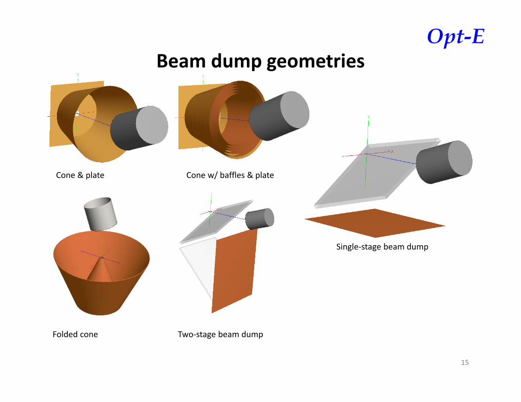
Opt-EBeam dump geometries

15

Cone & plate Cone w/ baffles & plate

Single‐stage beam dump

Two‐stage beam dumpFolded cone

Opt-EVisible beam dump comparison 

16

1.00E‐05

1.00E‐04

1.00E‐03

1.00E‐02

1.00E‐01

0 5 10 15 20

PST

off‐axis angle (deg)

Visible PST Trades

simple cone/flat

simple cone/gloss

cone w/cyl

stage 1 baffle

stage 2 baffle

nested cones

Opt-ELWIR beam dump comparison

17

1.00E‐06

1.00E‐05

1.00E‐04

1.00E‐03

1.00E‐02

0 2 4 6 8 10 12 14 16 18 20

PS

T

off-axis angle deg)

LWIR PST Trades

simple cone/flat black

cone w/cyl

stage 1 baffle

stage 2 baffle

nested cones

Opt-ESimplified SLDD CAD model

18

Left side shows the two halves of the SLDD instrument together, but with doors and covers removed. The right side shows the instrument opened for service. The cryogenic beam dump is on the left side and is comprised of two rectangular takes oriented vertically, and two triangular tanks set horizontally. The top tank is hidden. Plumbing, electronics and the source modules are not shown.

Opt-ESimplified model in FRED

19

Basic conclusion is that the instrument signature in the scatter signal of interest is dominated by contamination of the mirrors in the beam delivery system.

The mirrors are 1.5” diameter and 2” diameter flats and replicated OAPs from Newport. They are small enough to CO2 snow clean and then replace when that is inadequate.

Opt-ESLDD Frames

Picture showing 3 frames for SLDD. There is a single source side frame and two beam dump frames. One beam dump is being built with a cryogenic beam dump for use in the LWIR. The second beam dump is for visible light at ambient temperatures.

20

Opt-ESLDD Frames

March 11, 2013 – stages / UUT on left, cryo side in clean room on right. Acktar black foil not yet applied to beam dump

21

March 14, 2013 – behind clean room.

Opt-ESLDD Frames

Top tank undergoing cryogenic testing.

22

Opt-ESLDD Instrument

April 26, 2013 – stages / UUT side.

23

April 26, 2013 – behind clean room.

Source platform

Opt-E3 cabinets & room

CAD model of three cabinets on the left and the three cabinets below in the cleanroom.

24

CMM

4’x12’

Env ch.

Zygo

Opt-EVisible light beam dump & Celestron

25

Source benchAries 8.6 µm

Celestron C‐8

Visible laser is behind Aries 

Opt-ECryogenic beam dump

26

Acktar foil (blue wrapping)

Opt-ESLDD program – Raster

27

Live Video

Status

The Raster tab allows for a brute force scan of any combination of axes in any order. Think of it as a set of nested for loops. The motion control is part of the “master program”.

Opt-ESLDD program – Test specification

28

Live Video

Status

The Test specification tab allows for loading a test specification from a file and displays the programs interpretation of the specification.

Opt-EExample test specification

// sample SLDD test specification file# 21 July 2012

Begin Test HeaderTest Name, Sample TestTest Creator, Armand SperdutiTest CommentUUT Name, Test TelescopeUUT Model Number, 123456UUT Serial Number, SN4321

End Test Header

Begin FOV Table0 0 null 100.5 5 1.5 10 point 34.5 139.2 100.5 15 1.5 340 1.5 350 11.0 340 115.0 0 215.0 10 2 End FOV Table

29

Begin Aperture 1rect 33.5 150.0 290.5 350.0 25.0 X 5.0 Y 2End Aperture

Begin Aperture 2vert 33.5 150.0 290.5 2End Aperture

Begin Scan Definitionz1 50.5process FOV TableEnd Scan Definition

Opt-ESLDD program – Measurement type

30

Live Video

Status

The Measurement type is the operation performed on each image to determine if the image, or processed result, should be saved. The basic test is any pixel above a threshold value, although additional choices can be readily implemented in LabVIEW.

Opt-ESLDD program – Stage – manual control

31

Live Video

Status

Stage manual control provides necessary controls for setup operations. Full status information from the Aerotech Ensemble controller is available on a second tab.

Opt-ESLDD program – Stage – status

32

Live Video

Status

Stage  status provides complete status information by axis.

Opt-ESLDD program – Configuration ‐ Scan

33

Live Video

Status

Configuration  Scan sets the velocities for the Raster test.

Opt-ESLDD program – Configuration ‐ Sensor

34

Live Video

Status

Configuration  Sensor provides access to the sensor sub‐panel for the sensor “Active Node”. The sensor interface is a stand alone program loaded in a subpanel that provides detailed control. The Active Node approach allows for interfaces to virtually any standard or custom sensor to be implemented.

Opt-ESLDD program – Configuration ‐ Sensor

35

Live Video

Status

Configuration  Sensor provides access to the sensor sub‐panel for the sensor “Active Node”. The sensor interface is a stand alone program loaded in a subpanel that provides detailed control. The Active Node approach allows for interfaces to virtually any standard or custom sensor to be implemented.

Opt-ESLDD program – Configuration ‐ Source

36

Live Video

Status

Configuration  Source provides access to the sensor sub‐panel for the source “Active Node”. The source interface is a stand alone program loaded in a subpanel that provides detailed control. The Active Node approach allows for interfaces to virtually any standard or custom source to be implemented.

Opt-ESLDD program – Configuration ‐ Source

37

Live Video

Status

Configuration  Source provides access to the sensor sub‐panel for the source “Active Node”. The source interface is a stand alone program loaded in a subpanel that provides detailed control. The Active Node approach allows for interfaces to virtually any standard or custom source to be implemented.

Opt-ESLDD program – Configuration ‐ Program

38

Live Video

Status

Configuration  Program provides access to file directory specifications and other necessary stuff.

Opt-ERead Scan File (1)

39

SLDD saves image data and Read Scan File allows for examination of the data. It is intended to be modified for further analysis. It is easy to write equivalent programs in any environment, such as Matlab. Data is from the Celestron C‐8 amateur telescope with a Basler Ace camera attached.

Opt-ERead Scan File (2)

40

SLDD saves image data and Read Scan File allows for examination of the data. It is intended to be modified for further analysis. It is easy to write equivalent programs in any environment, such as Matlab. Data is from the Celestron C‐8 amateur telescope with a Basler Ace camera attached.

Opt-ERead Scan File (3)

41

SLDD saves image data and Read Scan File allows for examination of the data. It is intended to be modified for further analysis. It is easy to write equivalent programs in any environment, such as Matlab. Data is from the Celestron C‐8 amateur telescope with a Basler Ace camera attached.

Opt-EWhat else to do?

• A control program to control filling of the cryogenic tanks needs to be written for the cryogenic beam dump.

• We are preparing to test the cryogenic beam dump in September. • We will test two IR&D telescopes at atmospheric temperature at both wavelengths this fall.• There are some miscellaneous hardware things to add such as AC power feeds, adding a shelf 

for the Aries laser controller, etc.• There are incremental software improvements and additions needed, as is usually true.

• Presentations or publications on measurement results compared with analyses, at least as possible, are also needed.

• We are looking to use this instrument, so please, talk to me. We can couple with stray light analysis if useful.

42

Opt-EBackup slides follow

43

Opt-E295 K BB, 0.03 e, 8‐12 µm (mirror)

44

Opt-E295 K BB, 1 e, 8‐12 µm (beam dump)

45

Opt-E100 K BB, 1.0 e, 8‐12 µm (beam dump)

46

Opt-E77.35 K BB, 1.0 e, 8‐12 µm (beam dump)

47

Opt-E6000 K BB, 1.0 e, 8‐12 µm  (sun)

48

Opt-E6000 K BB, 1.0 e, 0.4‐1 µm (sun)

49

Opt-E

50

Baffle PST Trades

Richard N. PfistererPhoton Engineering

Revised 16 Nov 2011

Opt-E

51

Analysis Technique

1. System under test is rotated about a fixed point in front of the baffle

2. Rays are traced from the system under test into a ±2 deg FOV. The source power is set to unity.

3. Rays are scattered back to the entrance aperture of the system under test

4. PST = (scatter power collected on entrance aperture)/(power emitted by entrance aperture)

Opt-E

52

Visible Flat Black Scatter Model

Opt-E

53

Visible Glossy Black Scatter Model

Opt-E

54

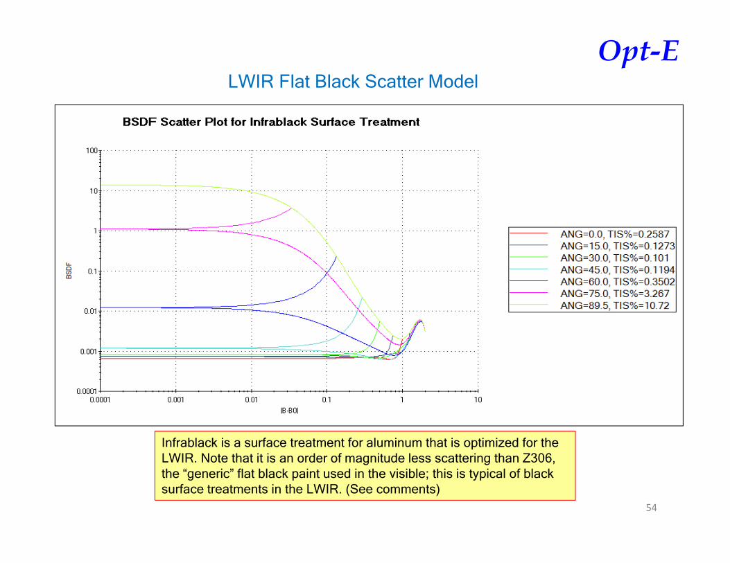
LWIR Flat Black Scatter Model

Infrablack is a surface treatment for aluminum that is optimized for the LWIR. Note that it is an order of magnitude less scattering than Z306, the “generic” flat black paint used in the visible; this is typical of black surface treatments in the LWIR. (See comments)

Opt-E

55

Simple Cone w/Flat Black Paint (Visible)

angle PST0 4.17E‐035 3.58E‐0310 2.23E‐0315 1.27E‐0320 8.27E‐04

Nothing exciting is happening here; this is the baseline calculation. Basically we’re looking at the scatter from a flat (diffuse) black surface.

Opt-E

56

Simple Cone w/Gloss Black Paint (Visible)

angle PST0 1.45E‐025 7.81E‐0310 7.45E‐0415 6.70E‐0520 6.73E‐05

Note that the near-normal PST is an order of magnitude higher than the flat black. This is due to the high specularityof the gloss paint creating a near-retro reflection back to the system under test. However once the system is tilted such that the reflection is outside the FOV, the PST drops an order of magnitude.

Opt-E

57

Simple Cone w/Cylindrical Baffles and Flat Black Paint (Visible)

There is not much difference in the PST between the flat black cone and the cone w/cylindrical baffles because the geometry really isn’t much different: at normal incidence the system under test is looking at the same flat surface and at higher angles of incidence, it is looking at another conical surface.Based on these results, I don’t expect to see anything significantly different if we angled the cylindrical baffles.

angle PST0 4.15E‐035 3.56E‐0310 2.21E‐0315 1.26E‐0320 6.98E‐04

Opt-E

58

Stage 1 Baffle w/Black Glass and Flat Black Paint Absorber (Visible)

Note the significant improvement over the flat black paint baffles! I assumed a visibly dirty glass plate (level 500) and a 17 angstrom rms roughness surface.

angle PST0 8.61E‐055 7.63E‐0510 6.91E‐0515 6.05E‐0520 5.36E‐05

Opt-E

59

Stage 1 Baffle w/Black Glass and Flat Black Paint Absorber(no particles on glass, Visible)

It is tempting to consider how good the stage 1 baffle could be if you could eliminate the particles. At small angles, the PST is a factor of 2x lower; at larger angles it is better by a factor of 5x.

angle PST (no particles)0 3.76E‐055 2.84E‐0510 2.05E‐0515 1.46E‐0520 1.02E‐05

Opt-E

60

Stage 2 Baffle w/Black Glass and Flat Black Paint Absorber (Visible)

You’ll notice that the stage 2 baffle is virtually identical to the stage 1 baffle, despite the increase in complexity. This is due to the significant contribution from particulate scatter on the first glass plate.

angle PST0 5.52E‐055 4.77E‐0510 4.34E‐0515 4.11E‐0520 3.80E‐05

Opt-E

61

Stage 2 Baffle w/Black Glass and Flat Black Paint Absorber(no particles on glass, Visible)

Without particles, we pick up a factor of 5x improvement at small angles, but an order of magnitude improvement at larger angles.

angle PST (no particles)0 1.26E‐055 8.86E‐0610 5.81E‐0615 3.60E‐0620 2.13E‐06

Opt-E

62

Nested Cones w/Gloss Black Paint (Visible)

A rather interesting “middle ground” between the conventional baffles and the stage 1 and 2 baffles.

Fundamentally it is a conical cavity but the paint is glossy, so at each ray intersection with the surface, you have a specular reflection and a diffuse component.

Opt-E

63

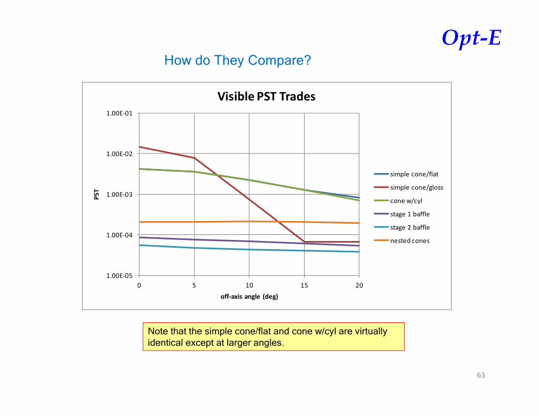
How do They Compare?

Note that the simple cone/flat and cone w/cyl are virtually identical except at larger angles.

1.00E‐05

1.00E‐04

1.00E‐03

1.00E‐02

1.00E‐01

0 5 10 15 20

PST

off‐axis angle (deg)

Visible PST Trades

simple cone/flat

simple cone/gloss

cone w/cyl

stage 1 baffle

stage 2 baffle

nested cones

Opt-E

64

Simple Cone w/Infrablack (LWIR)

This is approx. 4x lower than for the visible but the scatter mechanism is completely different: in the visible, the paint scatter is the dominant mechanism; in the LWIR, particulates contaminating the paint dominate and the paint is an insignificant contributor.

angle PST0 1.08E‐035 7.09E‐0410 3.03E‐0415 2.08E‐0420 2.16E‐04

Opt-E

65

Simple Cone w/Cylindrical Baffles and w/Infrablack (LWIR)

As before, there is not much difference in the PST between the flat black cone and the cone w/cylindrical baffles because the geometry really isn’t much different: at normal incidence the system under test is looking at the same flat surface and at higher angles of incidence, it is looking at another conical surface, both contaminated with particulates.

angle PST0 1.09E‐035 6.85E‐0410 2.87E‐0415 1.74E‐0420 1.65E‐04

Opt-E

66

Stage 1 Baffle w/Infrablack and w/Infrablack Absorber (LWIR)

Approx. 8x lower scatter than in the visible.

Note the significant improvement over the flat black paint baffles! I assumed a visibly dirty (Al?) panel (level 500) and a 17 angstrom rms roughness surface. However at this wavelength the surface scatter is entirely negligible.

angle PST0 1.07E‐055 9.34E‐0610 8.64E‐0615 8.14E‐0620 6.93E‐06

Opt-E

67

Stage 2 Baffle w/Black Glass and w/Infrablack Absorber (LWIR)

As before, you’ll notice that the stage 2 baffle is virtually identical to the stage 1 baffle, despite the increase in complexity. This is due to the significant contribution from particulate scatter on the first panel.

angle PST0 9.77E‐065 8.83E‐0610 7.71E‐0615 7.08E‐0620 6.13E‐06

Opt-E

68

Nested Cones w/InfraBlack (LWIR)

angle PST0 1.20E‐045 1.11E‐0410 1.07E‐0415 1.25E‐0420 1.39E‐04

A rather interesting “middle ground” between the conventional baffles and the stage 1 and 2 baffles.

Fundamentally it is a conical cavity but the paint is glossy, so at each ray intersection with the surface, you have a specular reflection and a diffuse component.

Opt-E

69

How do They Compare?

Note that the simple cone/flat and cone w/cyl are virtually identical except at larger angles.

1.00E‐06

1.00E‐05

1.00E‐04

1.00E‐03

1.00E‐02

0 2 4 6 8 10 12 14 16 18 20

PS

T

off-axis angle deg)

LWIR PST Trades

simple cone/flat black

cone w/cyl

stage 1 baffle

stage 2 baffle

nested cones

Opt-E

70

Visible and LWIR PST Comparisons

While you could certainly argue that this is an “apples and oranges” comparison, it does serve to illustrate quantitatively how visible and LWIR scatter compare due to different physical processes.

angle visible  LWIR visible  LWIR visible  LWIR visible  LWIR visible LWIR0 4.17E‐03 1.08E‐03 4.15E‐03 1.09E‐03 8.61E‐05 1.07E‐05 5.52E‐05 9.77E‐06 2.04E‐04 1.20E‐045 3.58E‐03 7.09E‐04 3.56E‐03 6.85E‐04 7.63E‐05 9.34E‐06 4.77E‐05 8.83E‐06 2.05E‐04 1.11E‐0410 2.23E‐03 3.03E‐04 2.21E‐03 2.87E‐04 6.91E‐05 8.64E‐06 4.34E‐05 7.71E‐06 2.15E‐04 1.07E‐0415 1.27E‐03 2.08E‐04 1.26E‐03 1.74E‐04 6.05E‐05 8.14E‐06 4.11E‐05 7.08E‐06 2.07E‐04 1.25E‐0420 8.27E‐04 2.16E‐04 6.98E‐04 1.65E‐04 5.36E‐05 6.93E‐06 3.80E‐05 6.13E‐06 1.94E‐04 1.39E‐04

simple cone/flat cone w/cyl stage 1 baffle stage 2 baffle nested cones

Opt-E

71

Comments

• The baffles geometries are simple.. because they are! Fundamentally there are two techniques for controlling scattered light:

1. Low scatter diffuse coatings2. High reflectivity gloss coatings or black mirrors where there is

controlled loss and controlled direction• Certainly “tweaking” is possible but I would not expect to see significant differences relative to these results.• Particulates are a driver in any low-scatter system, especially in LWIR.• Adding complexity (i.e., going to a stage 2 baffle) is probably not warranted if it cannot be kept very clean.• It’s going to take a bit of effort to find BRDF data for black paints in the LWIR. I was able to find some data on several LWIR black paints but not enough to create a valid scatter model. (Publishing scatter measurements of various paints and surface treatments is very much “out of style” these days; most of the scatter data I have is from the 1980’s and early 1990’s. Since so much information is now considered proprietary, the open literature is becoming less useful as a source of information.)