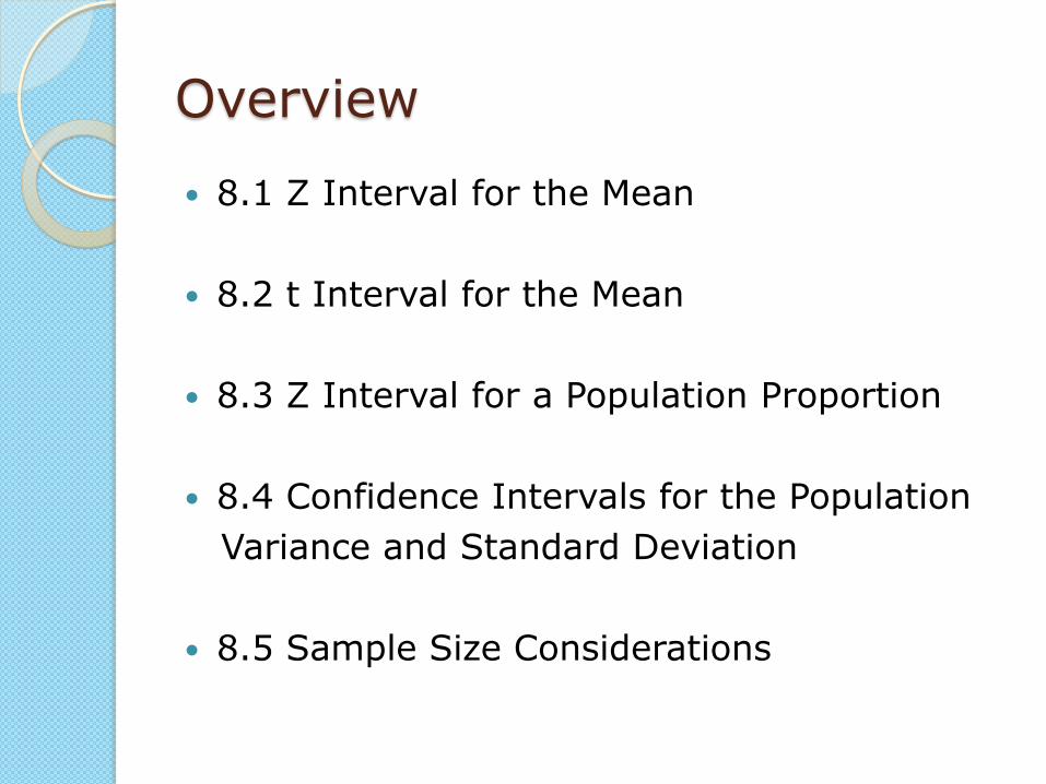
Overview

8.1 Z Interval for the Mean

8.2 t Interval for the Mean

8.3 Z Interval for a Population Proportion

8.4 Confidence Intervals for the Population

Variance and Standard Deviation

8.5 Sample Size Considerations

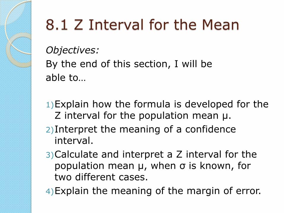
8.1 Z Interval for the Mean

Objectives:

By the end of this section, I will be

able to…

1)Explain how the formula is developed for the Z interval for the population mean μ.

2)Interpret the meaning of a confidence interval.

3)Calculate and interpret a Z interval for the population mean μ, when σ is known, for two different cases.

4)Explain the meaning of the margin of error.

Introduction to confidence intervals

Confidence interval estimate - consists of an

interval of numbers generated by a point

estimate together with an associated

confidence level specifying the probability

that the interval contains the parameter

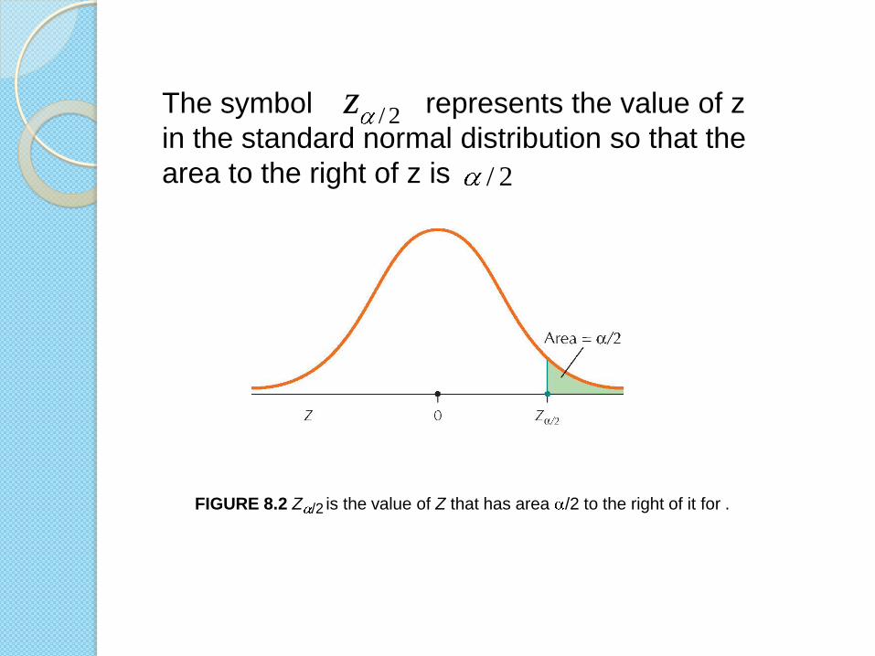
FIGURE 8.2 Z is the value of Z that has area /2 to the right of it for . /2

2/zThe symbol represents the value of z

in the standard normal distribution so that the

area to the right of z is 2/

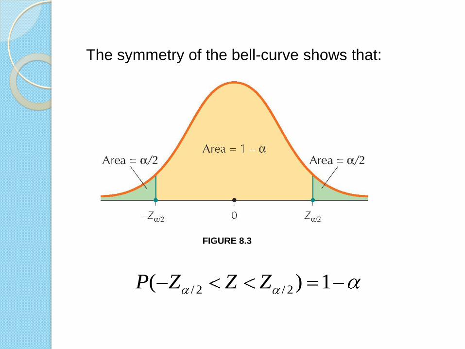
FIGURE 8.3

The symmetry of the bell-curve shows that:

1)( 2/2/ ZZZP

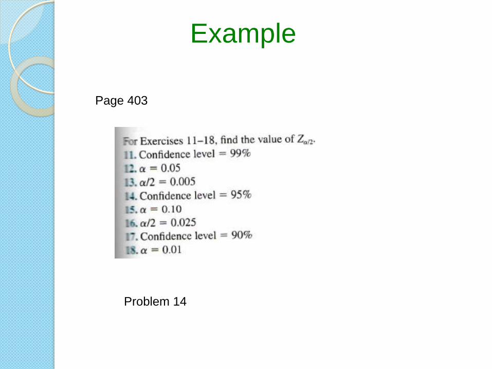
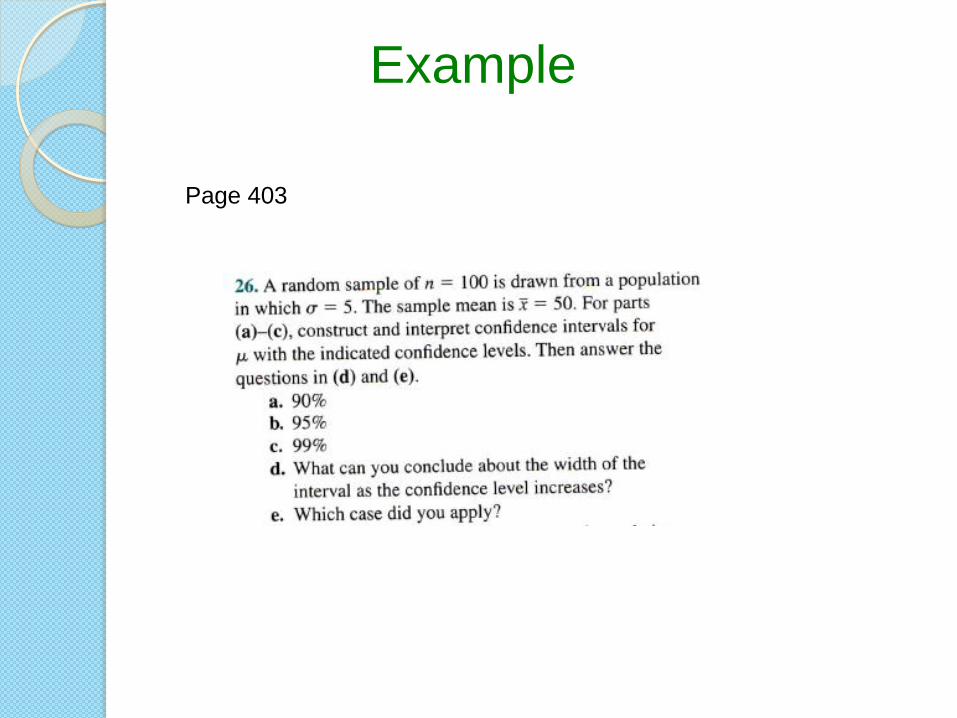
Example

Page 403

Problems 12 and 16

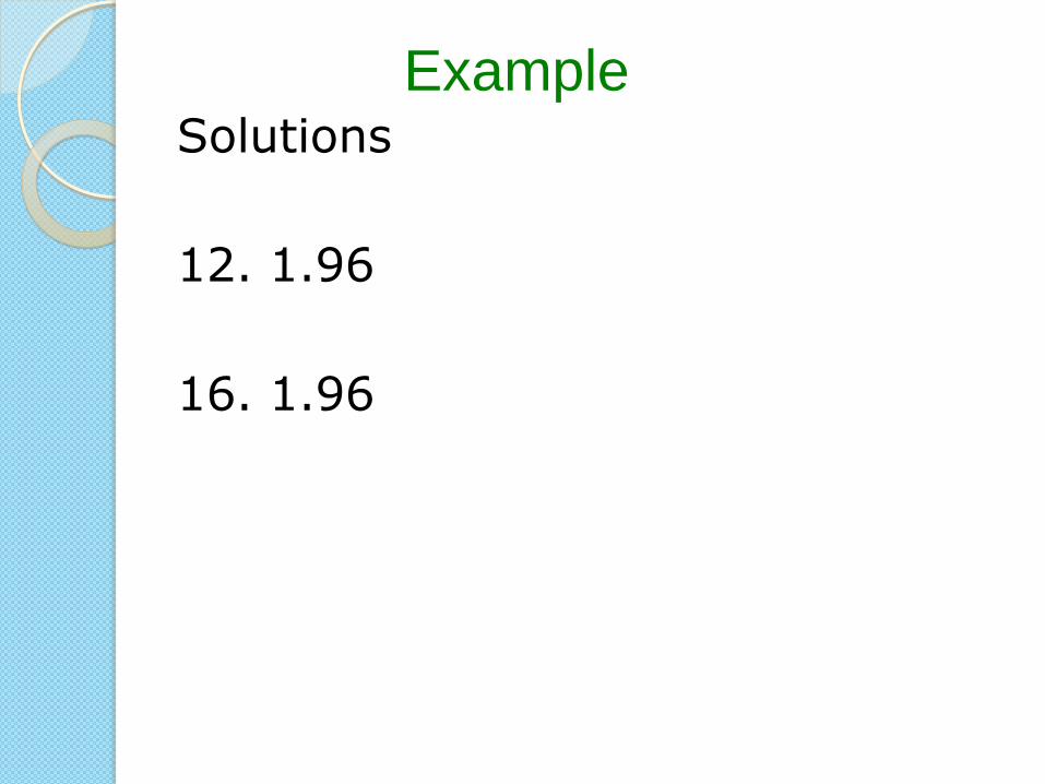
Solutions

12. 1.96

16. 1.96

Example

Recall from chapter 7, Central Limit Theorem

The sampling distribution of the sample mean for a normal population or any population if sample size is at least 30 is distributed as normal with mean:

And standard deviation:

x

nx /

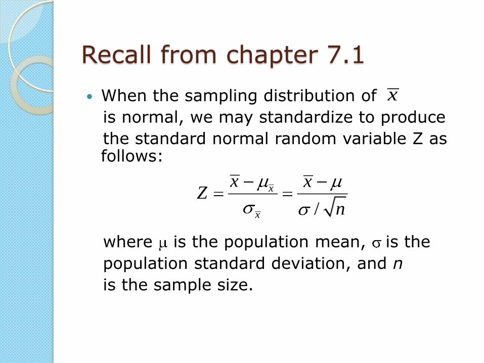
Recall from chapter 7.1

When the sampling distribution of

is normal, we may standardize to produce

the standard normal random variable Z as follows:

where is the population mean, is the

population standard deviation, and n

is the sample size.

/

x

x

x xZ

n

x

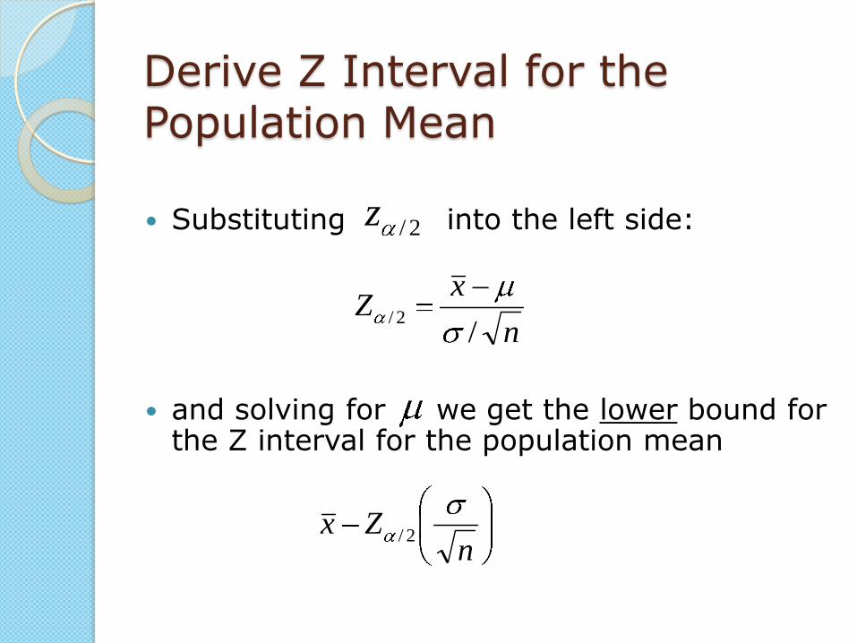
Derive Z Interval for the Population Mean

Substituting into the left side:

and solving for we get the lower bound for the Z interval for the population mean

2/z

nZx 2/

n

xZ

/2/

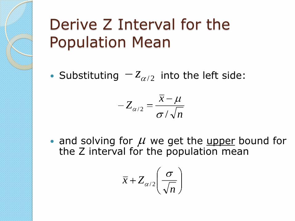
Derive Z Interval for the Population Mean

Substituting into the left side:

and solving for we get the upper bound for the Z interval for the population mean

2/z

nZx 2/

n

xZ

/2/

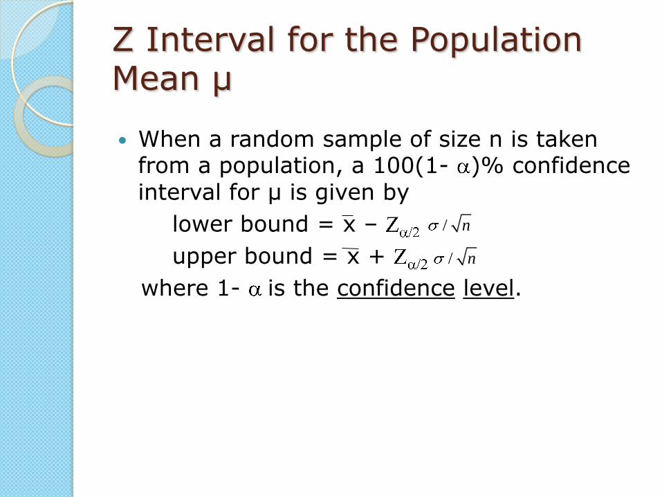
Z Interval for the Population Mean μ

When a random sample of size n is taken from a population, a 100(1- )% confidence interval for μ is given by

lower bound = x –

upper bound = x +

where 1- is the confidence level.

/ n

/ n

Z Interval for the Population Mean μ

The Z interval can also be written as confidence interval (CI)

nZx

nZxCI 2/2/ ,

Example

Page 403

Problem 14

Solution

14. 1.96

Example

z 2 for a 95% Confidence Level

2 = 2.5% = .025 = 5%

TABLE 8.1 Z /2 values for common confidence levels

Z Interval for the Population Mean μ

Used only under certain conditions

Case 1:

Population is normally distributed

The value of σ is known

Case 2:

n ≥ 30

The value of σ is known

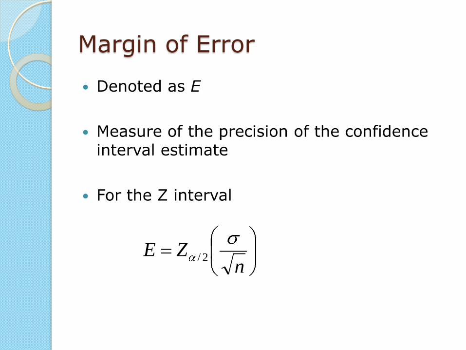
Margin of Error

Denoted as E

Measure of the precision of the confidence interval estimate

For the Z interval

nZE 2/

Interpreting the Margin of Error

For a (1 - )100% confidence interval for μ

“We can estimate μ to within E units with

(1 - )100% confidence.”

Interpreting the Confidence Interval

Page 393

Example

Page 403

Solutions

(a)Case 2 applies

(b) 1

(c) 1.96

Example

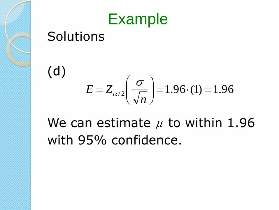
Solutions

(d)

We can estimate to within 1.96

with 95% confidence.

Example

96.1)1(96.12/n

ZE

Solutions

(e)

CI=(18.04,21.96)

Example

04.1896.1202/n

Zx

96.2196.1202/n

Zx

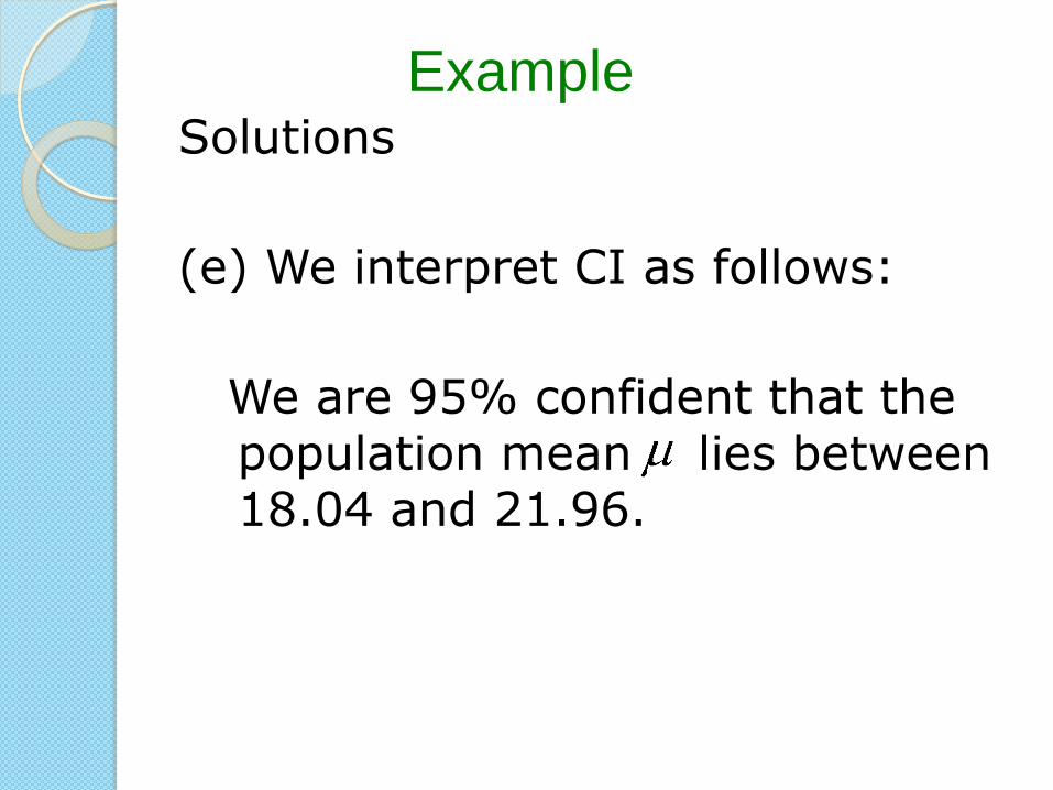
Solutions

(e) We interpret CI as follows:

We are 95% confident that the population mean lies between 18.04 and 21.96.

Example

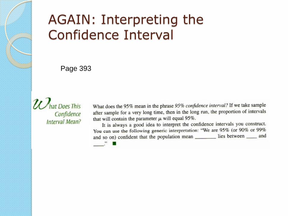
AGAIN: Interpreting the Confidence Interval

Page 393

Example

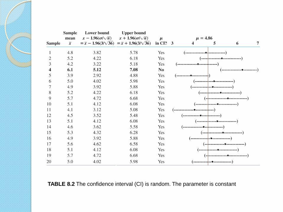
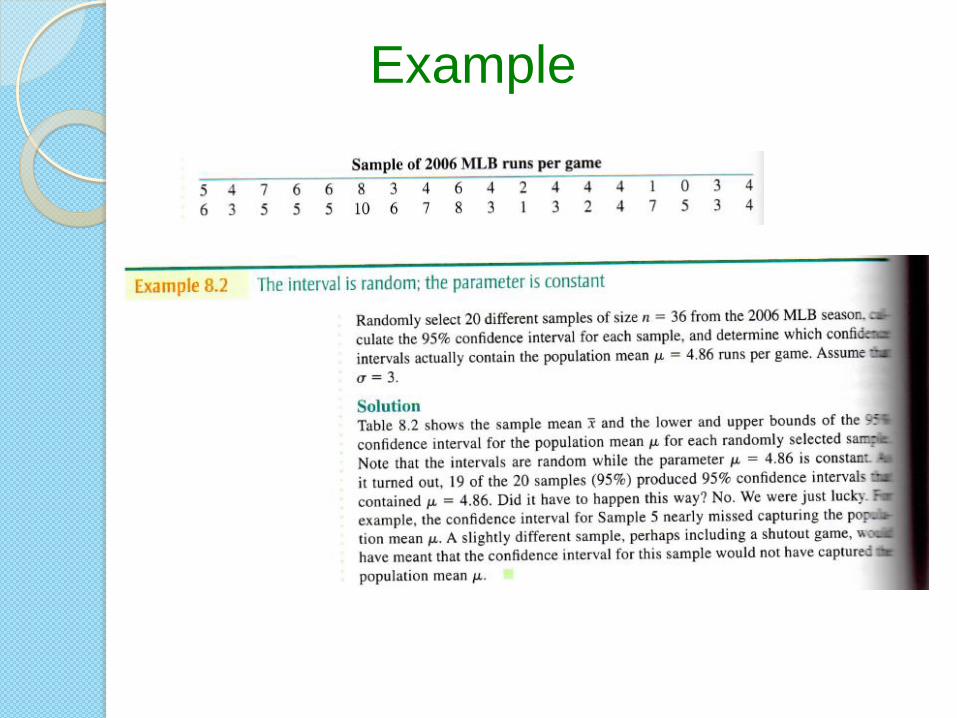
TABLE 8.2 The confidence interval (CI) is random. The parameter is constant

Example

Page 403

TABLE 8.1 Z /2 values for common confidence levels

RECALL

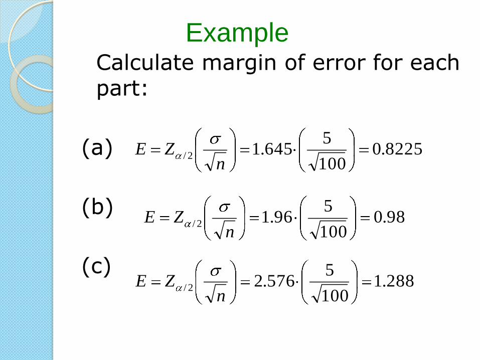
Calculate margin of error for each part:

(a)

(b)

(c)

Example

8225.0100

5645.12/

nZE

98.0100

596.12/

nZE

288.1100

5576.22/

nZE

Solutions

(a)

CI=(49.1775,50.8225)

Example

1775.498225.0502/n

Zx

8225.518225.0502/n

Zx

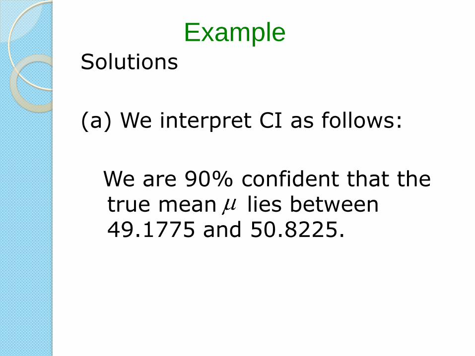
Solutions

(a) We interpret CI as follows:

We are 90% confident that the true mean lies between 49.1775 and 50.8225.

Example

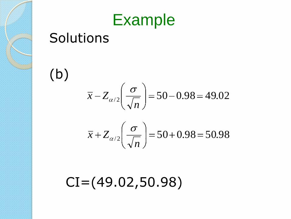
Solutions

(b)

CI=(49.02,50.98)

Example

02.4998.0502/n

Zx

98.5098.0502/n

Zx

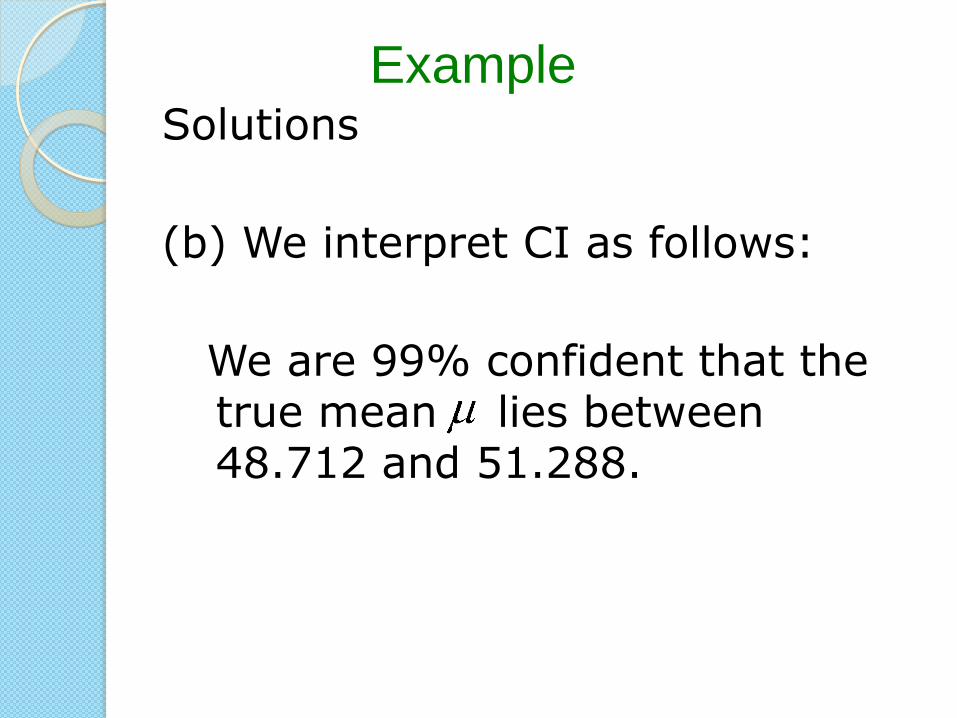
Solutions

(b) We interpret CI as follows:

We are 95% confident that the true mean lies between 49.02 and 50.98.

Example

Solutions

(c)

CI=(48.712,51.288)

Example

712.48288.1502/n

Zx

288.51288.1502/n

Zx

Solutions

(b) We interpret CI as follows:

We are 99% confident that the true mean lies between 48.712 and 51.288.

Example

Solutions

(d) The confidence interval for a given sample size gets wider as the confidence level increases

(e) Case 2: the sample size is large, and the value of σ is known

Example

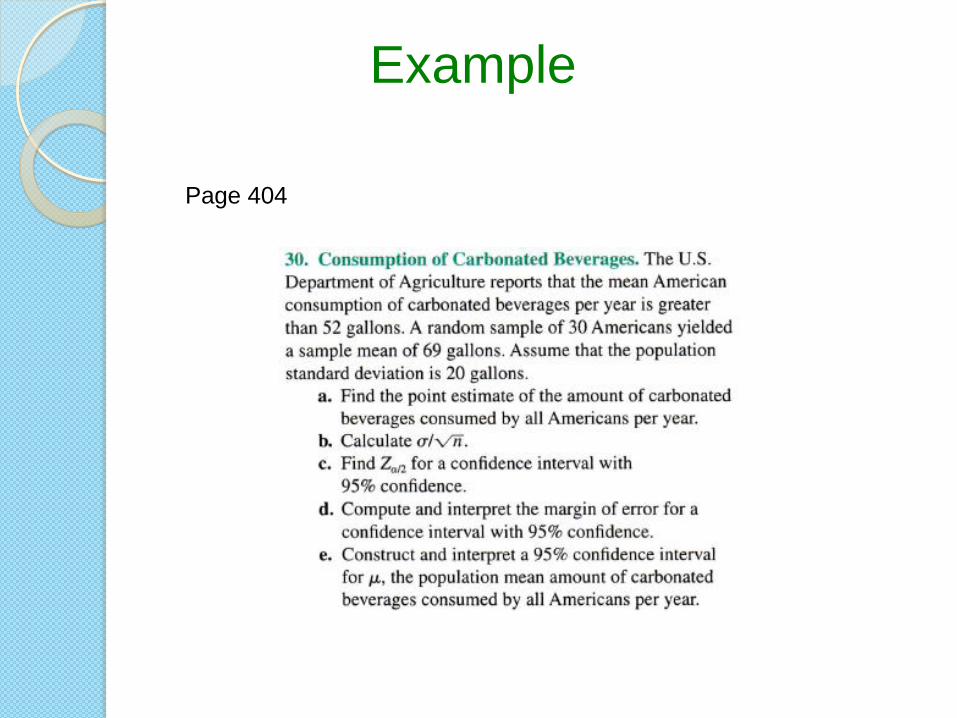
Example

Page 404

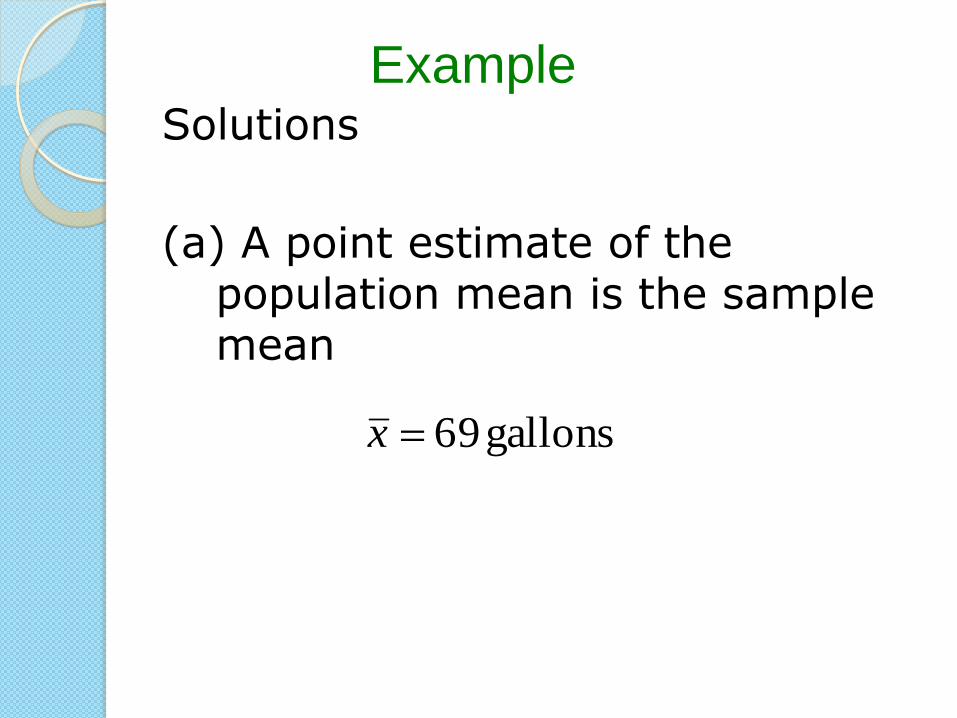
Solutions

(a) A point estimate of the population mean is the sample mean

Example

gallons 69x

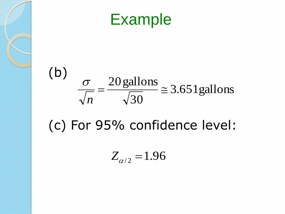
(b)

(c) For 95% confidence level:

Example

gallons 651.330

gallons 20

n

96.12/Z

(d) Margin of error

We can estimate the population mean to within 7.16 gallons with 95% confidence.

Example

gallons 16.7)651.3(96.12/n

ZE

Solutions

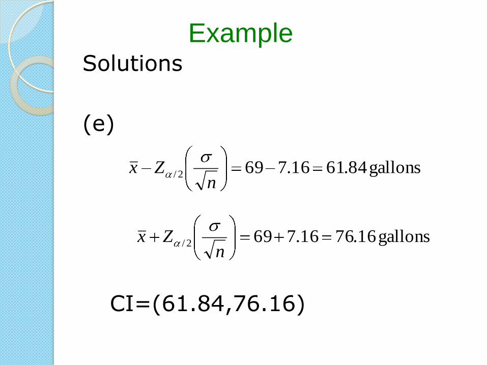
(e)

CI=(61.84,76.16)

Example

gallons 84.6116.7692/n

Zx

gallons 16.7616.7692/n

Zx

Solutions

(e) We interpret CI as follows:

We are 95% confident that the true mean lies between 61.84 gallons and 76.16 gallons.

Example

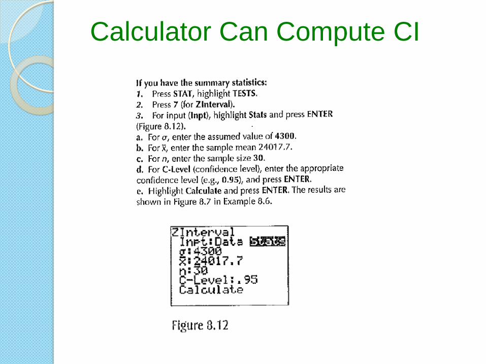
Calculator Can Compute CI

Summary

A confidence interval estimate of a parameter consists of an interval of numbers generated by a point estimate, together with an associated confidence level specifying the probability that the interval contains the parameter.

The meaning of a 100(1 confidence interval is as follows: If we take sample after sample for a very long time, then in the long run, the proportion of intervals that will contain the parameter μ will equal 100 100(1 - )%.

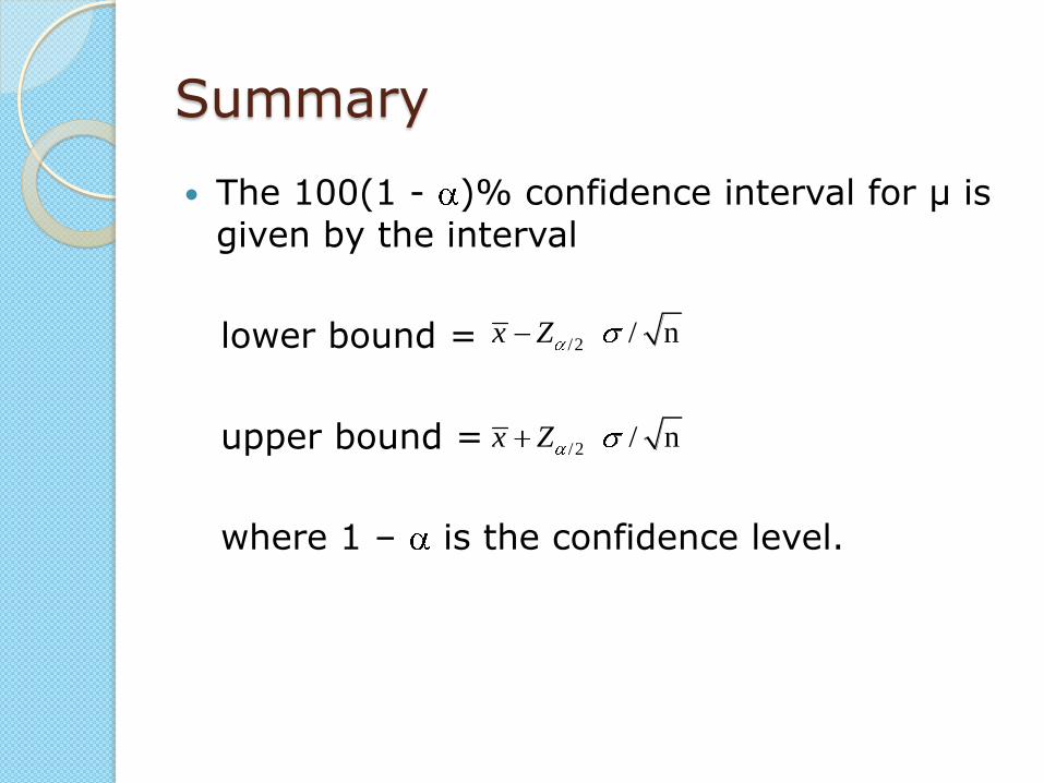
Summary

The 100(1 - )% confidence interval for μ is given by the interval

lower bound =

upper bound =

where 1 – is the confidence level.

/2 / nx Z

/2 / nx Z

Summary

The conditions for applying this confidence interval are as follows:

Case 1:

The original population is normal and σ is

known.

Case 2:

The sample size is large (n ≥ 30) and σ is known.

Summary

If σ is not known, then the Z interval cannot be used.

The margin of error E is a measure of the precision of the confidence interval estimate.

For the Z interval, the margin of error takes the form

2

E Zn

Summary

We interpret the margin of error E for a (1 - )100% confidence interval for μ as follows:

“We can estimate to within E with (1 - )100% confidence.”

Confidence intervals often take the form

point estimate ± margin of error

8.2 t Interval for the Mean

Objectives:

By the end of this section, I will be

able to…

1) Describe the characteristics of the t distribution.

2) Calculate and interpret a t interval for the mean, for either of two cases.

3) Compute and interpret the standard error.

t Distribution

In real-world problems, σ is often unknown

Use s to estimate the value of σ

For a normal population

follows a t distribution

/

xt

s n

t Distribution continued

n - 1 degrees of freedom (df)

Where x is the sample mean

μ is the unknown population mean

s is the sample standard deviation

n is the sample size

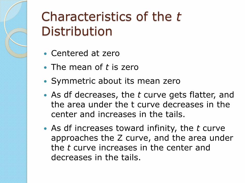
Characteristics of the t Distribution

Centered at zero

The mean of t is zero

Symmetric about its mean zero

As df decreases, the t curve gets flatter, and the area under the t curve decreases in the center and increases in the tails.

As df increases toward infinity, the t curve approaches the Z curve, and the area under the t curve increases in the center and decreases in the tails.

FIGURE 8.13 Different t curve for different degrees of freedom (df n 1).

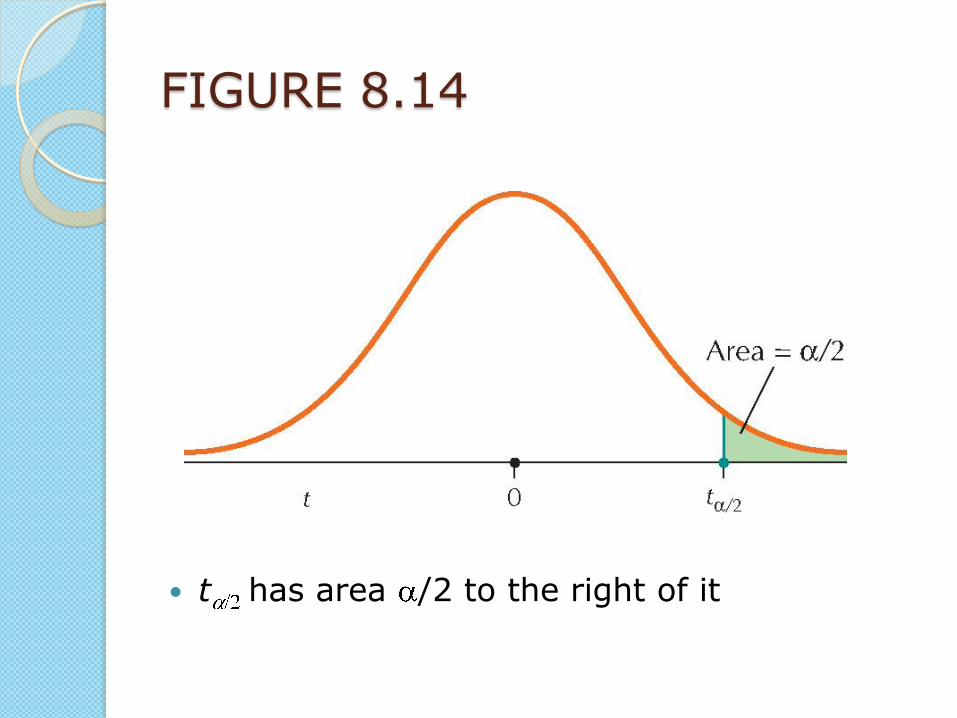
FIGURE 8.14

t has area /2 to the right of it

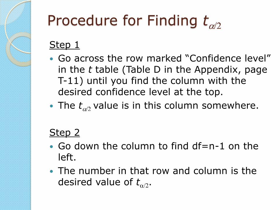
Procedure for Finding t

Step 1

Go across the row marked “Confidence level” in the t table (Table D in the Appendix, page T-11) until you find the column with the desired confidence level at the top.

The t value is in this column somewhere.

Step 2

Go down the column to find df=n-1 on the left.

The number in that row and column is the desired value of t .

Example 8.11 - Finding t

Find the value of t that will produce a 95%

confidence interval for μ if the sample

size is n = 20.

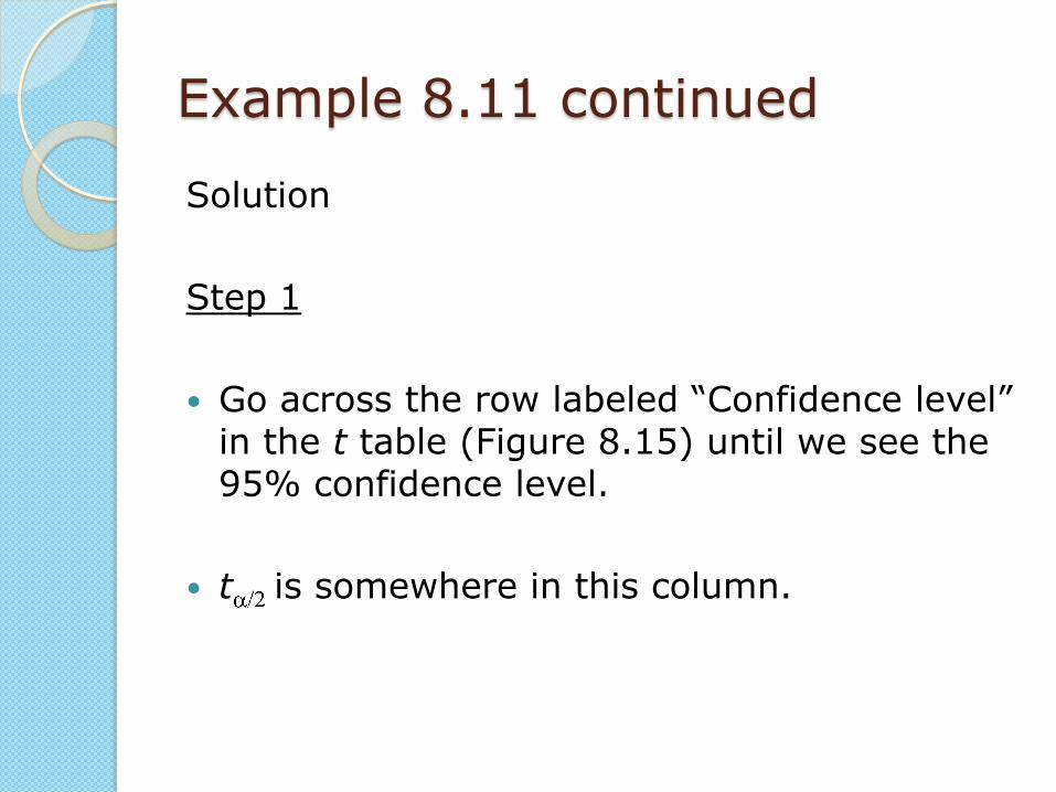
Example 8.11 continued

Solution

Step 1

Go across the row labeled “Confidence level” in the t table (Figure 8.15) until we see the 95% confidence level.

t is somewhere in this column.

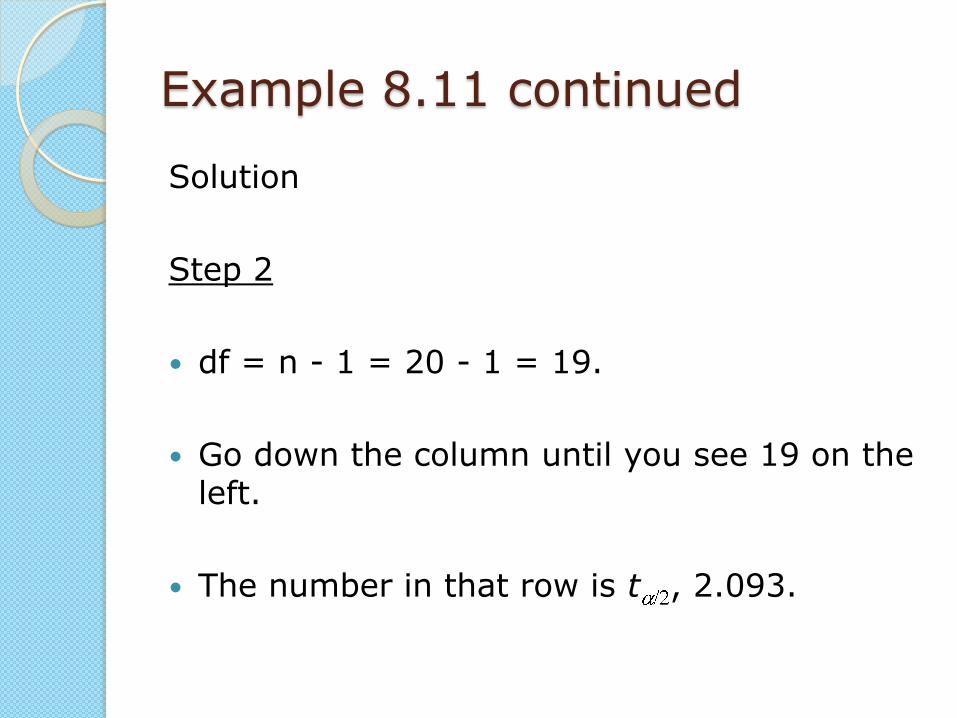
Example 8.11 continued

Solution

Step 2

df = n - 1 = 20 - 1 = 19.

Go down the column until you see 19 on the left.

The number in that row is t , 2.093.

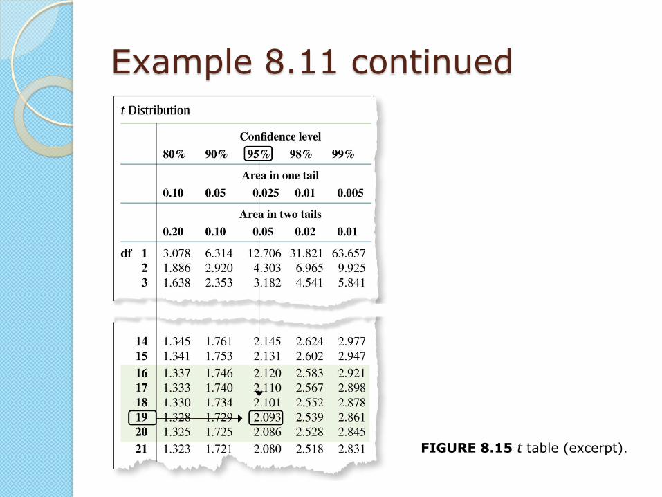
Example 8.11 continued

FIGURE 8.15 t table (excerpt).

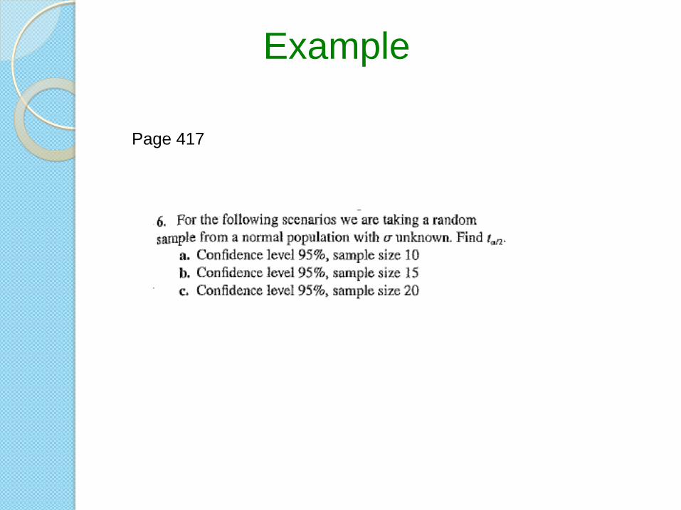
Example

Page 417

(a) 2.262 (note: df=9)

(b) 2.145 (note: df=14)

(c) 2.093 (note: df=19)

Example

t Interval for μ

Random sample of size n

Unknown mean μ

Confidence interval for μ

lower bound ,

upper bound

x is the sample mean

t is associated with the confidence level

n - 1 degrees of freedom

s is the sample standard deviation.

/2 /x t s n

/2 /x t s n

The t interval may also be written as confidence interval (CI)

n

stx

n

stxCI 2/2/ ,

t Interval for μ

t Interval for μ continued

The t interval applies whenever either of the following conditions is met:

Case 1:

The population is normal.

Case 2:

The sample size is large (n ≥ 30).

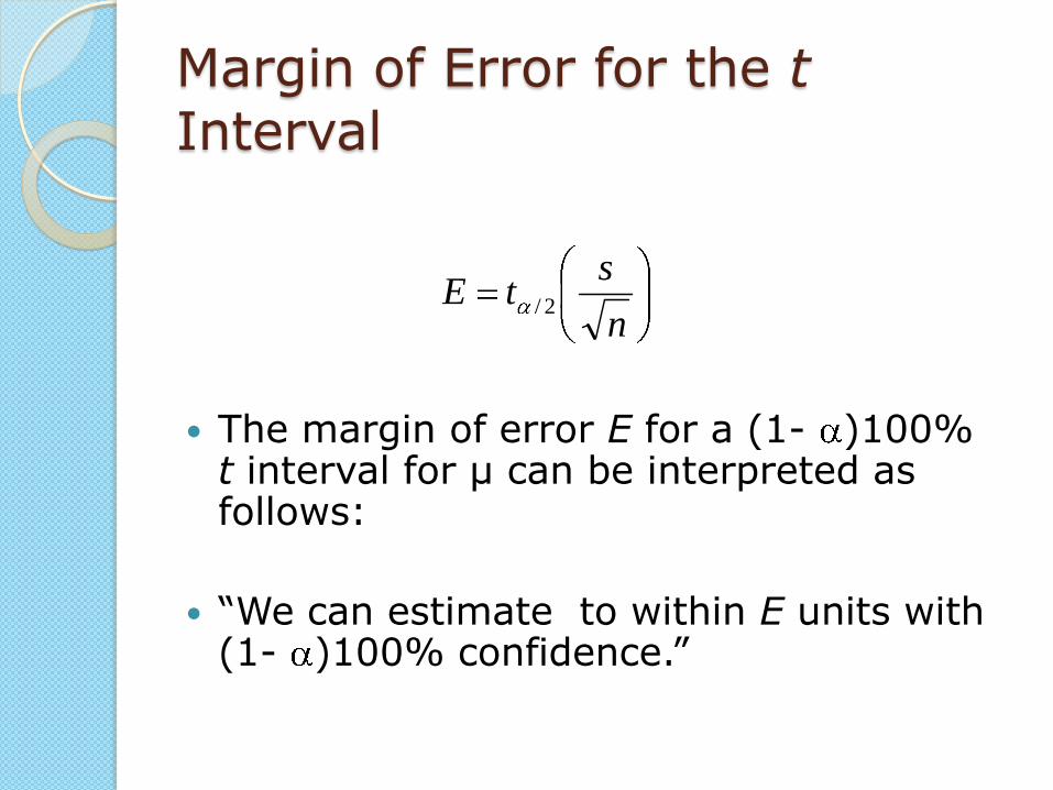
Margin of Error for the t Interval

The margin of error E for a (1- )100%

t interval for μ can be interpreted as follows:

“We can estimate to within E units with (1- )100% confidence.”

n

stE 2/

Example

Page 417

Problem 14

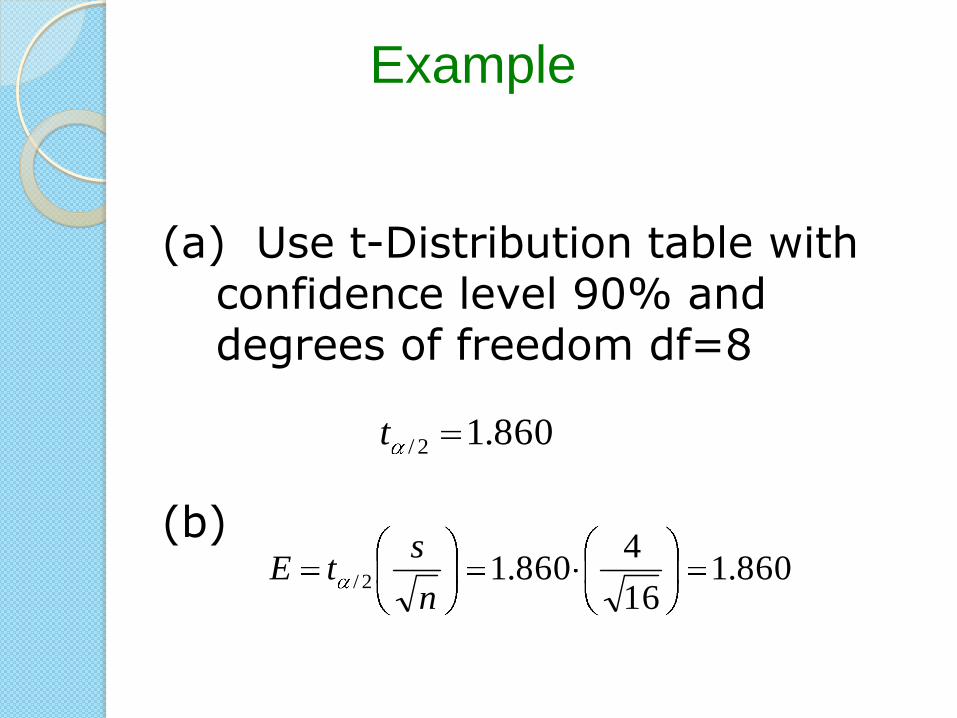
(a) Use t-Distribution table with confidence level 90% and degrees of freedom df=8

(b)

Example

860.116

4860.12/

n

stE

860.12/t

Solutions

(c)

CI=(20.140,23.860)

Example

140.20860.1222/n

stx

860.23860.1222/n

stx

Example

Page 417

Problem 26

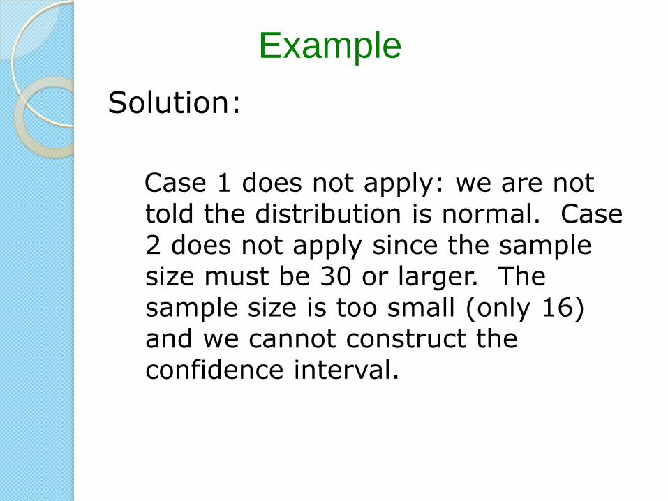
Solution:

Case 1 does not apply: we are not told the distribution is normal. Case 2 does not apply since the sample size must be 30 or larger. The sample size is too small (only 16) and we cannot construct the confidence interval.

Example

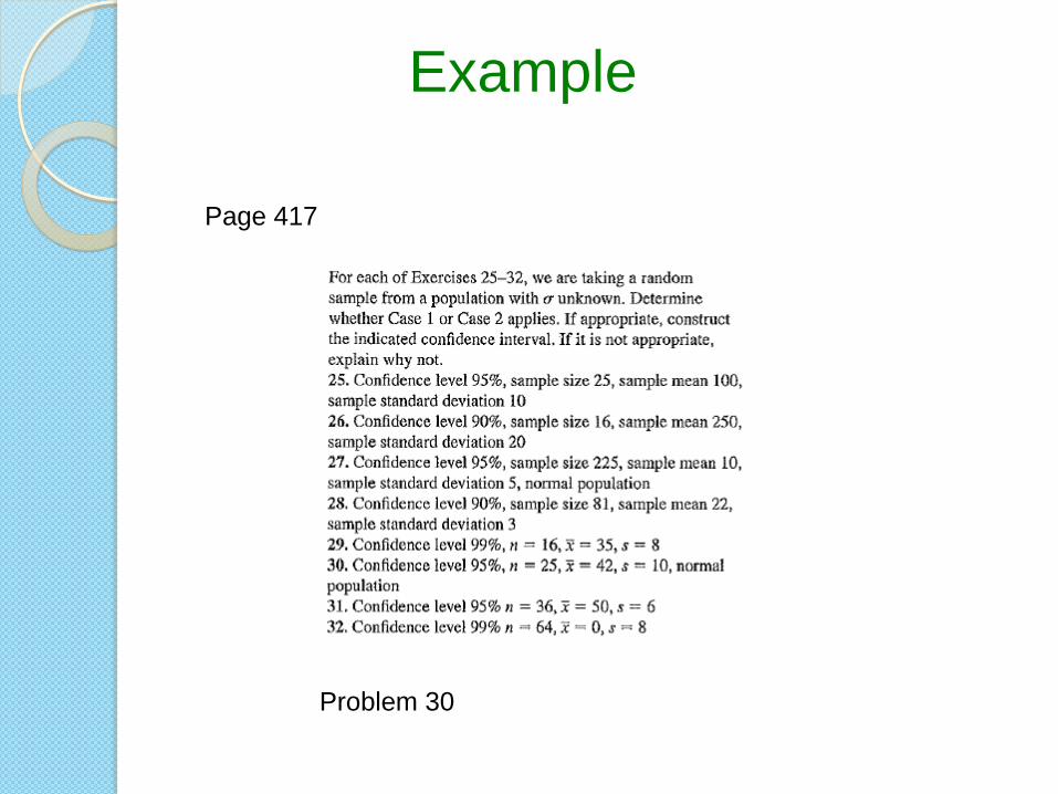
Example

Page 417

Problem 30

Solution:

Case 1 does apply: we are told the distribution is normal. We can construct the confidence interval.

Example

(a) Use t-Distribution table with confidence level 95% and degrees of freedom df=24

Margin of error:

Example

128.425

10064.22/

n

stE

064.22/t

CI=(37.872,46.128)

Example

872.37128.4422/n

stx

128.46128.4422/n

stx

Example

Page 418

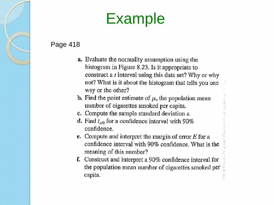
Example

Page 418

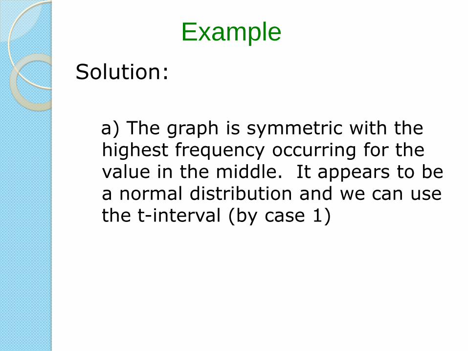
Solution:

a) The graph is symmetric with the highest frequency occurring for the value in the middle. It appears to be a normal distribution and we can use the t-interval (by case 1)

Example

Solution:

parts (b) and (c) can be determined by entering the data in a list in the calculator and using:

STAT CALC 1:1-Var Stats

b) the sample mean is

c) sample standard deviation:

Example

25.2392x

59.274s

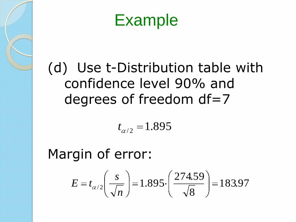
(d) Use t-Distribution table with confidence level 90% and degrees of freedom df=7

Margin of error:

Example

97.1838

59.274895.12/

n

stE

895.12/t

e) CI=(2208.28,2576.22)

Example

28.220897.18325.23922/n

stx

22.257697.18325.23922/n

stx

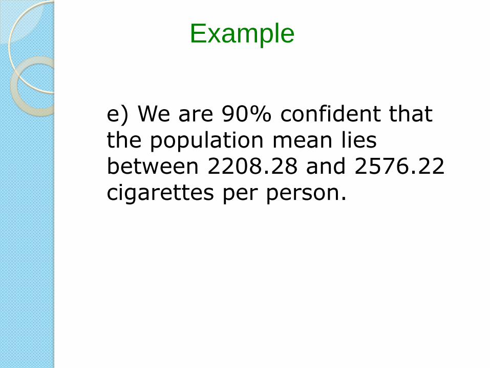
e) We are 90% confident that the population mean lies between 2208.28 and 2576.22 cigarettes per person.

Example

Calculator Can Compute CI

Summary

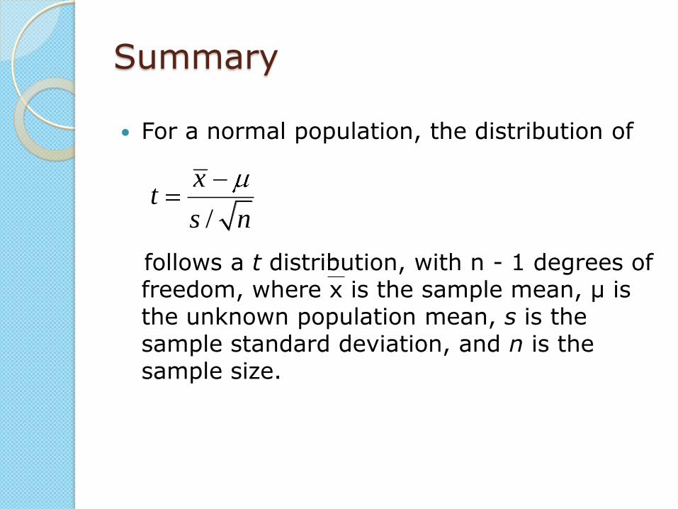
For a normal population, the distribution of

follows a t distribution, with n - 1 degrees of freedom, where x is the sample mean, μ is the unknown population mean, s is the sample standard deviation, and n is the sample size.

/

xt

s n

Summary

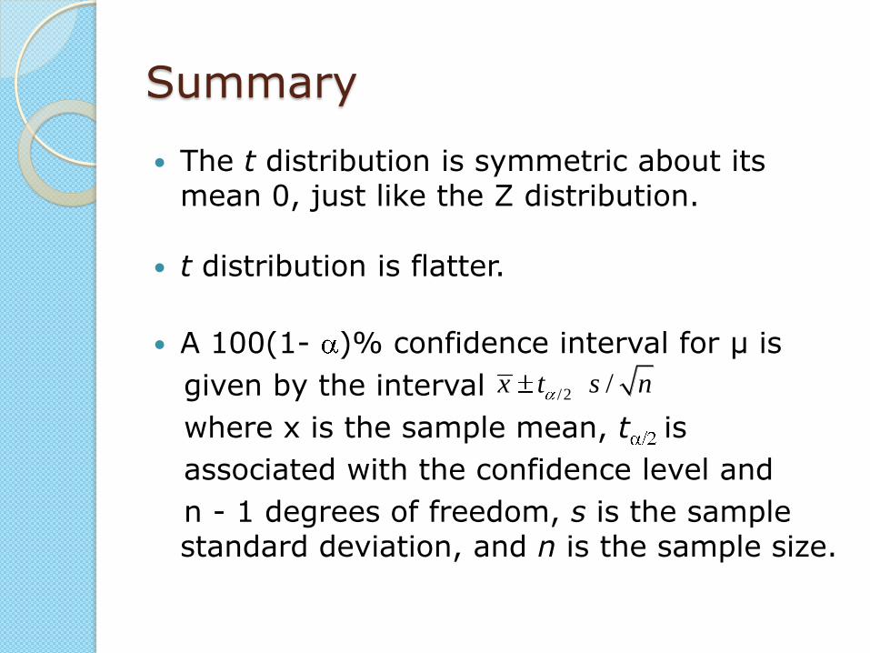
The t distribution is symmetric about its mean 0, just like the Z distribution.

t distribution is flatter.

A 100(1- )% confidence interval for μ is

given by the interval

where x is the sample mean, t is

associated with the confidence level and

n - 1 degrees of freedom, s is the sample standard deviation, and n is the sample size.

/2 /x t s n

Summary

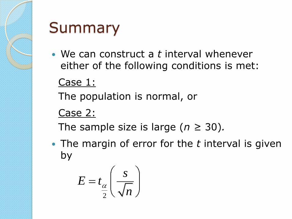
We can construct a t interval whenever either of the following conditions is met:

Case 1:

The population is normal, or

Case 2:

The sample size is large (n ≥ 30).

The margin of error for the t interval is given by

2

sE t

n

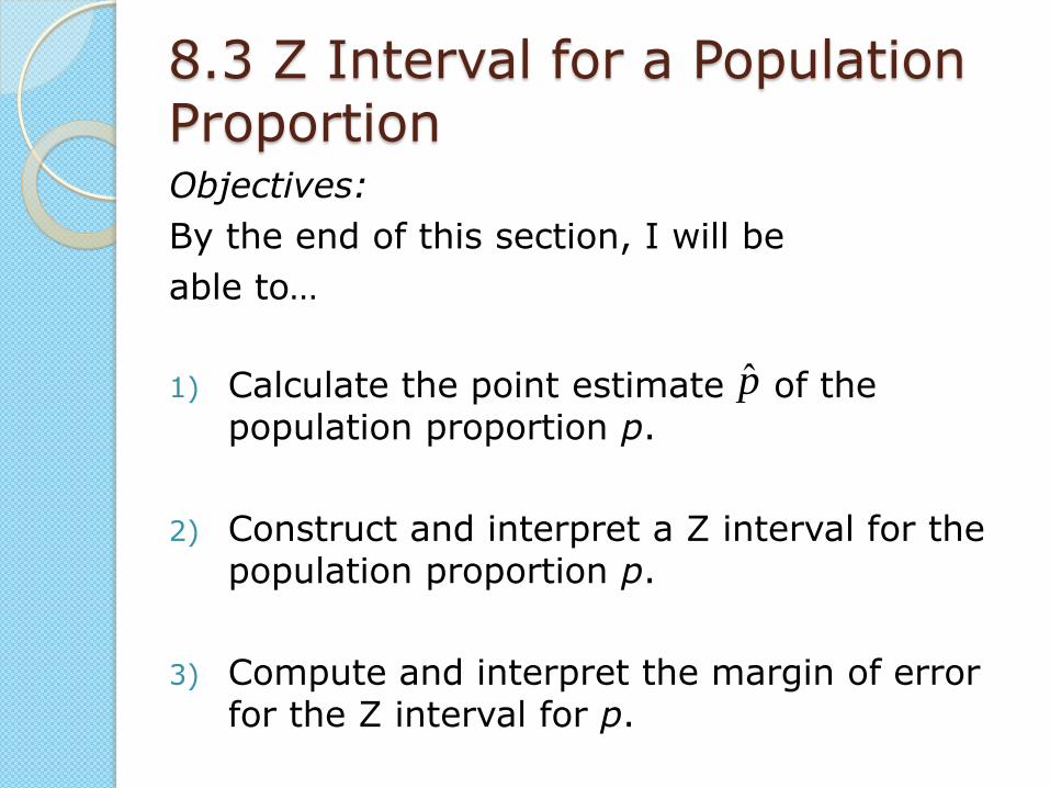
8.3 Z Interval for a Population Proportion Objectives:

By the end of this section, I will be

able to…

1) Calculate the point estimate of the population proportion p.

2) Construct and interpret a Z interval for the population proportion p.

3) Compute and interpret the margin of error for the Z interval for p.

p̂

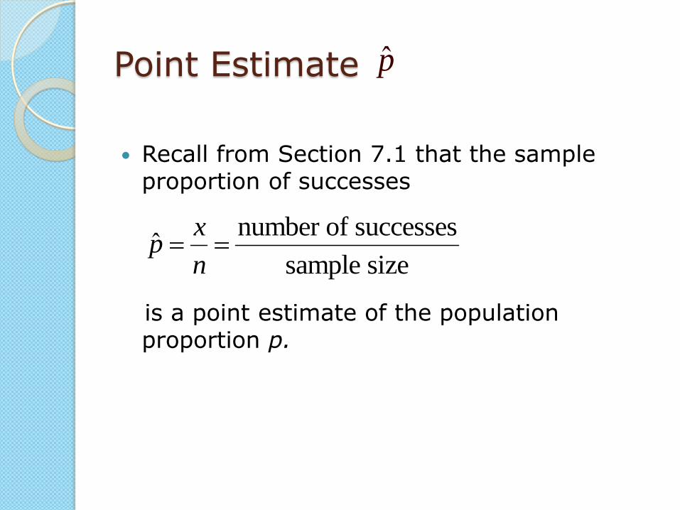
Point Estimate

Recall from Section 7.1 that the sample proportion of successes

is a point estimate of the population proportion p.

p̂

number of successesˆ

sample size

xp

n

Central Limit Theorem for Proportions

The sampling distribution of the sample proportion p follows an approximately normal distribution with mean μp = p

standard deviation

When both the following conditions are satisfied: (1) np ≥ 5 and (2) n(1 - p) ≥ 5.

1p

p p

n

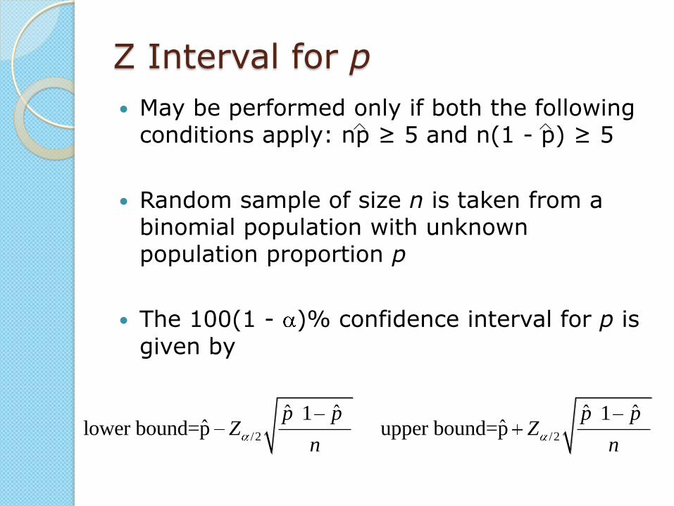
Z Interval for p

May be performed only if both the following conditions apply: np ≥ 5 and n(1 - p) ≥ 5

Random sample of size n is taken from a binomial population with unknown population proportion p

The 100(1 - )% confidence interval for p is given by

/2

ˆ ˆ1ˆlower bound=p

p pZ

n/2

ˆ ˆ1ˆupper bound=p

p pZ

n

Z Interval for p continued

Alternatively

Where p is the sample proportion of successes, n is the sample size, and

depends on the confidence level

/2

ˆ ˆ1ˆ

p pp Z

n

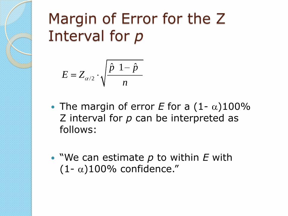
Margin of Error for the Z Interval for p

The margin of error E for a (1- )100% Z interval for p can be interpreted as follows:

“We can estimate p to within E with (1- )100% confidence.”

/2

ˆ ˆ1p pE Z

n

TABLE 8.1 Z /2 values for common confidence levels

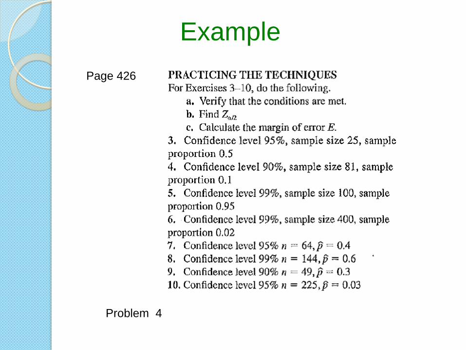
Example

Page 426

Problem 4

Solution

4(a)

Example

51.8)1.0(81p̂n

59.71)9.0(81ˆ)ˆ1( qnpn

Solution

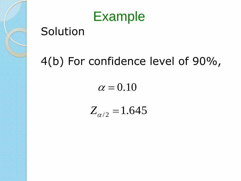
4(b) For confidence level of 90%,

Example

10.0

645.12/Z

Solution

4(c)

Example

0548.0

81

)90.0(10.0645.1

ˆˆ)ˆ1(ˆ2/2/

n

qpZ

n

ppZE

Example

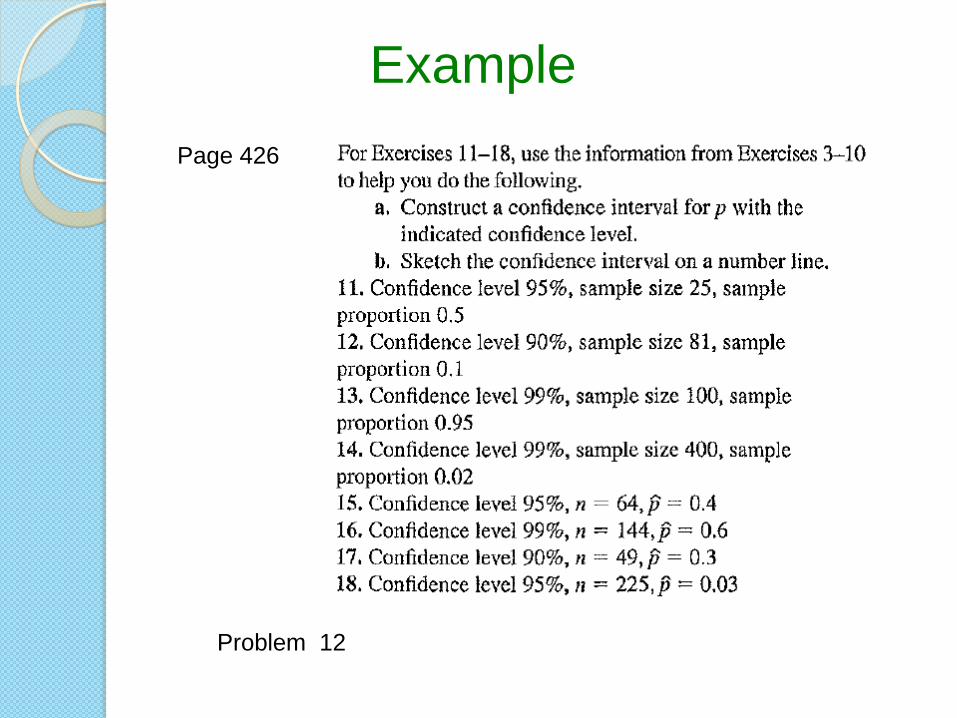
Page 426

Problem 12

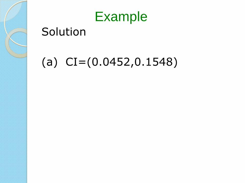
Solution

(a) CI=(0.0452,0.1548)

Example

Example

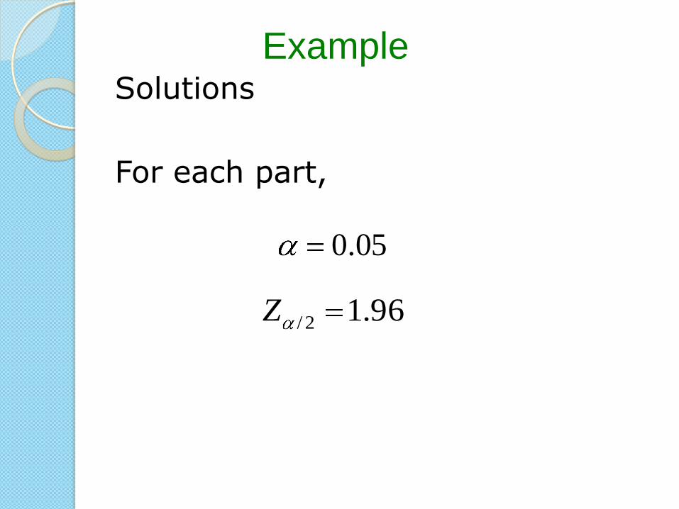
Solutions

For each part,

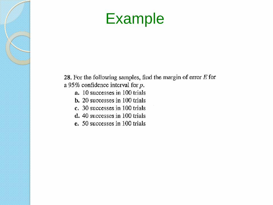
Example

05.0

96.12/Z

Solution

(a)

Example

0588.0100

)90.0(10.096.1

ˆˆ2/

n

qpZE

10.0100

10p̂

Solution

(b)

Example

0784.0100

)80.0(20.096.1

ˆˆ2/

n

qpZE

20.0100

20p̂

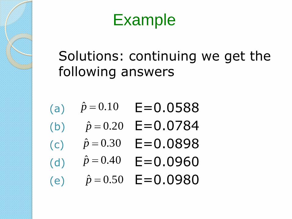
Solutions: continuing we get the following answers

(a) E=0.0588

(b) E=0.0784

(c) E=0.0898

(d) E=0.0960

(e) E=0.0980

Example

10.0p̂

20.0p̂

30.0p̂

40.0p̂

50.0p̂

Example

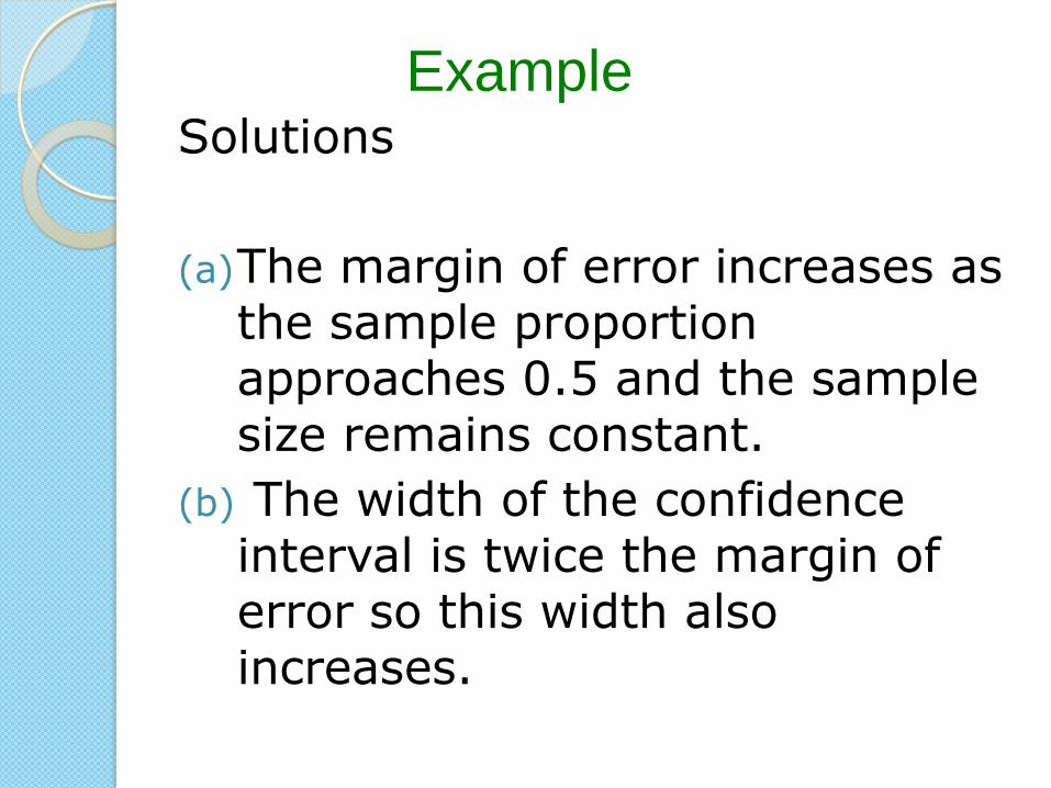
Solutions

(a)The margin of error increases as the sample proportion approaches 0.5 and the sample size remains constant.

(b) The width of the confidence interval is twice the margin of error so this width also increases.

Example

Example

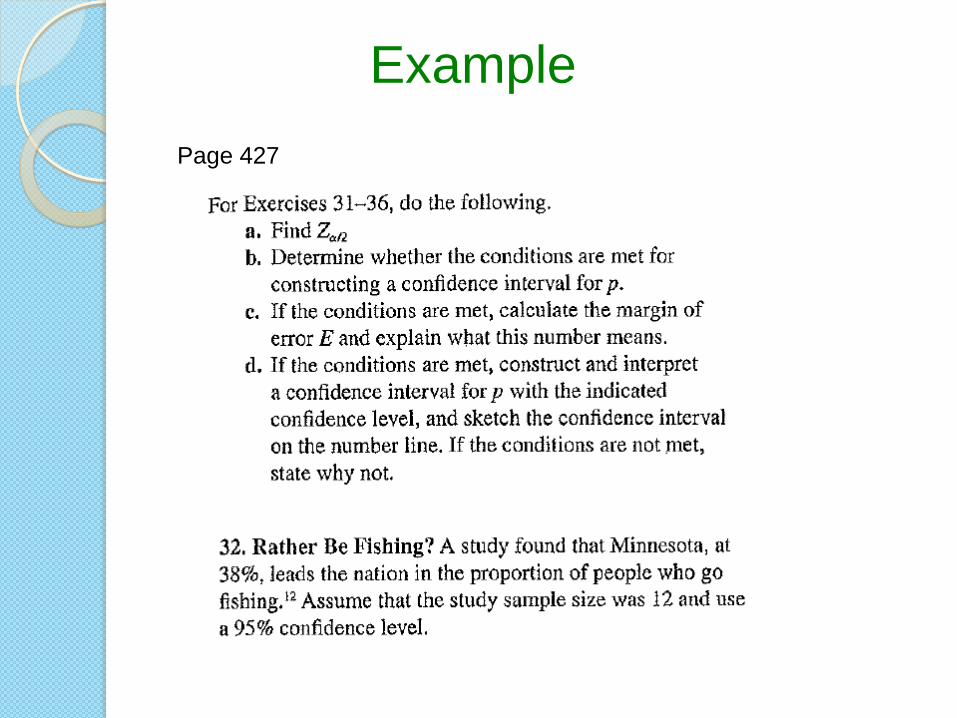
Page 427

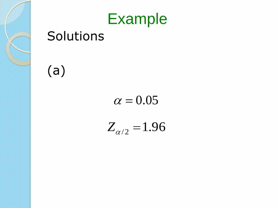
Solutions

(a)

Example

05.0

96.12/Z

Solution

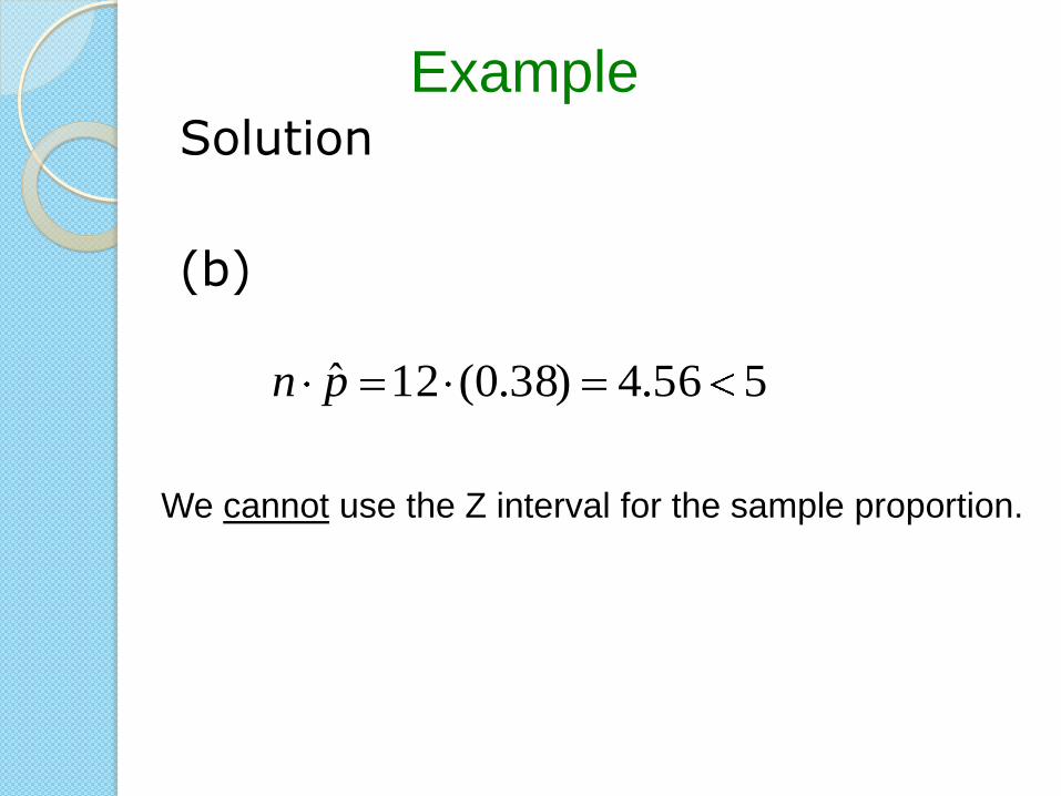
(b)

Example

556.4)38.0(12p̂n

We cannot use the Z interval for the sample proportion.

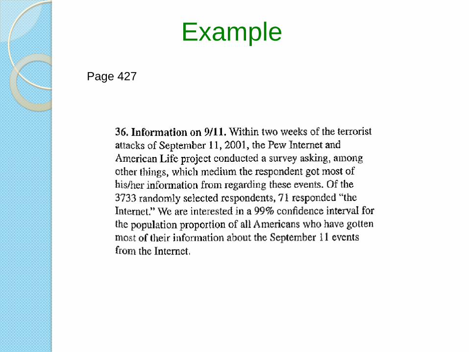
Example

Page 427

Solutions

(a)

Example

01.0

576.22/Z

(b)

Example

571)0190.0(3733p̂n

0190.03733

71p̂

53662)981.0(3733)0190.01(3733q̂n

We can use the Z interval for the sample proportion.

(c)

We can estimate the population proportion

within 0.0058 with 99% confidence.

Example

0058.03733

)981.0(0190.0576.2

ˆˆ2/

n

qpZE

0190.03733

71p̂

(d)

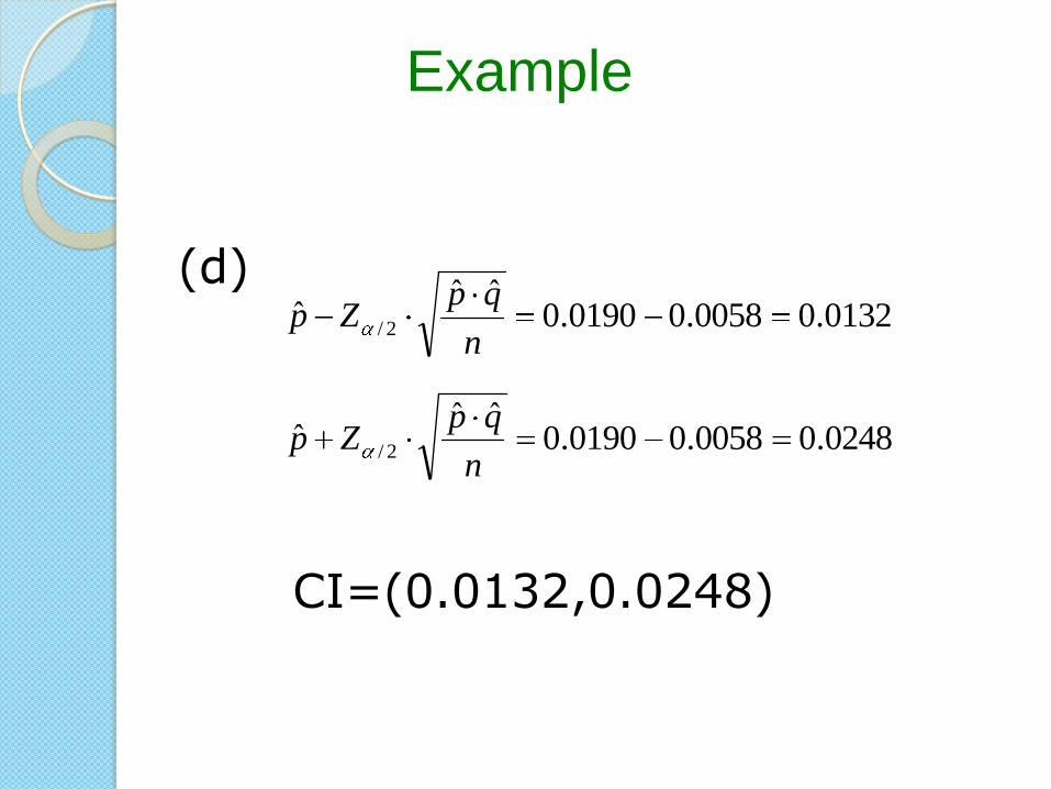
CI=(0.0132,0.0248)

Example

0132.00058.00190.0ˆˆ

ˆ2/

n

qpZp

0248.00058.00190.0ˆˆ

ˆ2/

n

qpZp

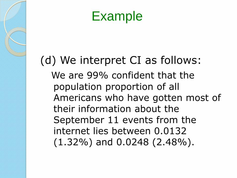
(d) We interpret CI as follows:

We are 99% confident that the

population proportion of all Americans who have gotten most of their information about the September 11 events from the internet lies between 0.0132 (1.32%) and 0.0248 (2.48%).

Example

Calculator Can Compute CI

Summary

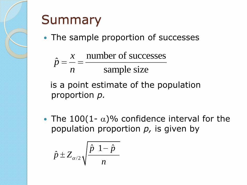
The sample proportion of successes

is a point estimate of the population

proportion p.

The 100(1- )% confidence interval for the population proportion p, is given by

number of successesˆ

sample size

xp

n

/2

ˆ ˆ1ˆ

p pp Z

n

Summary

Where p is the sample proportion of

successes, n is the sample size, and

depends on the confidence level.

The Z interval for p may be constructed only

if both the following conditions apply:

n p ≥ 5 and n(1 - p) ≥ 5.

Summary

Note that the confidence interval for p takes

on the form point estimate ± margin of error

where p is the point estimate of p and

is the margin of error. /2ˆ ˆ1 /aE Z p p n