OVERVIEW QDENSITY/QCWAVE: AMATHEMATICA QUANTUM COMPUTER

SIMULATION.

Frank Tabakina

a Department of Physics and AstronomyUniversity of Pittsburgh, Pittsburgh, PA, 15260

tabakin@pitt.edu

Abstract

The Mathematica quantum computer simulation packages QDENSITY andQCWAVE are extensively extended and upgraded. The density matrix is fea-tured in QDENSITY while in QCWAVE a quantum state vector approach isstressed. The present versions are provided in several associated packages;namely, QDensity, QCWave, BTSystem and Circuits . Tutorials are presented,some of which update earlier ones, plus several new ones that illustrate thecapabilities of the packages.

This version includes improved treatment of tensor products of states anddensity matrices, based on new features that are included in Mathematica 9- 10.3. A major extension to include qutrit (triplet), as well as qubit(binary)and hybrid qubit/qutrit systems is described in tutorials and in the associatedBTSystem package. Many other new features are also illustrated in tutorialnotebooks. Updated sample quantum computation algorithms and entangle-ment studies are presented, including Schmidt decomposition, entropy, mutualinformation, partial transposition, and calculation of the quantum discord. Ex-amples of Bell’s theorem are also included. These extensions and upgrades willhopefully be instructive and also aid in studies of QC dynamics, stability, andefficacy of error correction methods.

Preprint submitted to Elsevier December 12, 2015

Contents

1 INTRODUCTION 4

2 Qubit and Qutrit States 42.1 Single Qubit and Qutrit states . . . . . . . . . . . . . . . . . . . 52.2 Multi-Qubit and Qutrit states . . . . . . . . . . . . . . . . . . . . 5

2.2.1 Two-Qubit states . . . . . . . . . . . . . . . . . . . . . . . 72.2.2 Two-Qutrit states . . . . . . . . . . . . . . . . . . . . . . 72.2.3 Hybrid Qubit - Qutrit ( BT) states . . . . . . . . . . . . 10

3 Qubit and Qutrit Gates 123.1 Single-Qubit Basis . . . . . . . . . . . . . . . . . . . . . . . . . . 123.2 Multi-Qubit Operator Basis . . . . . . . . . . . . . . . . . . . . 143.3 Single-Qutrit Basis and Gates . . . . . . . . . . . . . . . . . . . 153.4 Multi-Qutrit Basis and Gates . . . . . . . . . . . . . . . . . . . . 193.5 Qubit-Qutrit Operators . . . . . . . . . . . . . . . . . . . . . . . 243.6 General Operators . . . . . . . . . . . . . . . . . . . . . . . . . . 25

3.6.1 General Qubit Operators . . . . . . . . . . . . . . . . . . 253.6.2 General Qutrit Operators . . . . . . . . . . . . . . . . . . 253.6.3 General BT Hybrid Operators . . . . . . . . . . . . . . . 25

4 Entanglement 294.1 Schmidt decomposition . . . . . . . . . . . . . . . . . . . . . . . 294.2 Entropy, mutual information, Quantum Discord . . . . . . . . . 31

4.2.1 Partial Trace . . . . . . . . . . . . . . . . . . . . . . . . 334.2.2 Discord . . . . . . . . . . . . . . . . . . . . . . . . . . . 33

4.3 Partial Transposition . . . . . . . . . . . . . . . . . . . . . . . . 344.4 Bell’s theorem . . . . . . . . . . . . . . . . . . . . . . . . . . . . 34

5 Other new aspects 355.1 QC algorithms & Simulations . . . . . . . . . . . . . . . . . . . 35

6 Future Plans: Parallel & Cuda versions 35

A Tutorials 38

2

List of Figures

1 Single qubit states. DForm and DFormA display qubit kets andbras. . . . . . . . . . . . . . . . . . . . . . . . . . . . . . . . . . . 6

2 Single qutrit states. DFormT and DFormTA display qutrit ketsand bras. . . . . . . . . . . . . . . . . . . . . . . . . . . . . . . . 6

3 Two qubit states. DForm and DFormA display two-qubit ketsand bras. . . . . . . . . . . . . . . . . . . . . . . . . . . . . . . . 9

4 Two qutrit states. DFormT and DFormTA display two-qutritkets and bras. . . . . . . . . . . . . . . . . . . . . . . . . . . . . . 9

5 Multi-qubit states using the KetV command. . . . . . . . . . . . 106 A hybrid qubit-qutrit state. DFormBT (DFormBTA) display hy-

brid BT kets (bras). Subscripts indicate if the entry is a qubit orqutrit. . . . . . . . . . . . . . . . . . . . . . . . . . . . . . . . . . 10

7 A hybrid QA= B,B,T,B,T state . . . . . . . . . . . . . . . 118 A hybrid or Mixed Radix QA= B,T,T,B,B,T,T state. . . . 119 Qubit: Pauli and projection operators. . . . . . . . . . . . . . . 1310 Qubit: Hadamard operator. . . . . . . . . . . . . . . . . . . . . 1411 Qubit: CNOT and Toffoli gates. . . . . . . . . . . . . . . . . . . 1512 Qutrit Basis—Spin-one case . . . . . . . . . . . . . . . . . . . . . 1613 Qutrit Basis—Gell-Mann case . . . . . . . . . . . . . . . . . . . . 1714 Qutrit Basis—Generalized Pauli . . . . . . . . . . . . . . . . . . 1815 Qutrit Basis—NOT gate . . . . . . . . . . . . . . . . . . . . . . . 1816 Qutrit Basis—the qutrit Hadamard HT . . . . . . . . . . . . . . . 1917 Multi-qutrit basis and the SPT command . . . . . . . . . . . . . 2018 Two qutrit Hadamards on two qutrits . . . . . . . . . . . . . . . 2119 Qubit swap gates . . . . . . . . . . . . . . . . . . . . . . . . . . . 2320 Qutrit swap gates based on CNOT1 & CNOT2 failure. . . . . . . 2321 Qutrit swap gates based on CNOTH success . . . . . . . . . . . . 2422 General qubit operators, Hadamard example. . . . . . . . . . . . 2623 General qutrit operator examples . . . . . . . . . . . . . . . . . . 2724 General hybrid BT operator examples . . . . . . . . . . . . . . . 2825 Additional hybrid BT operator examples . . . . . . . . . . . . . . 2826 Schmidt decomposition for a random 2 qubit state m. . . . . . . 3027 Mutual Information example for a random BT density matrix Ω. 3128 Discord example. Here Ω is a random 2-qubit density matrix, I

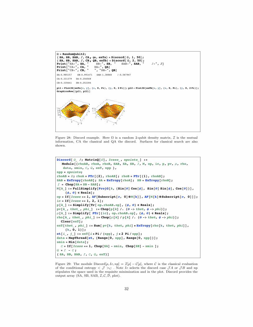
is the mutual information, CA the classical and QA the discord.Surfaces for classical search are also shown. . . . . . . . . . . . . 32

29 The module Discord[ρ, Ic, np] = I[ρ]−C[ρ], where C is the classi-cal evaluation of the conditional entropy < J >C . Note Ic selectsthe discord case JA or JB and np stipulates the space used inthe requisite minimization and in the plot. Discord provides theoutput array (SA, SB, SAB, I, C,D, plot). . . . . . . . . . . . . 32

3

1. INTRODUCTION

This is an overview of the 2015 version of a flexible simulation of a quantumcomputer; namely, the Mathematica(MM) packages QDensity [1], QCWave [2].These packages have been greatly improved and extended. A Fortran-90 quan-tum computer (QC) simulation package called QCMPI has been published [3],which uses parallel processing and message passing interface(MPI) capabilities.Some features of that work have been included in our present MM renditions. 1

In our earlier papers, we described qubit state vectors and associated am-plitudes for one, two and multi-qubit states and methods for handling one, twoand three-qubit operators or gates acting on state vectors. The basic idea ofa density matrix and its formation have also been described earlier. For guid-ance with these ideas and a description of our notation and usage, we refer thereader to our earlier works. We have attempted to maintain consistent and clearnotation to aid the user.

In the present paper, we first describe qubit, qutrit and hybrid (mixed qubit& qutrit) states in section 2. In section 3, the qubit gates are reviewed andextended to qutrit and hybrid networks. The methods used to evaluate entropy,mutual information, partial trace, quantum discord, partial transpose, and Bell’stheorem are presented in section 4. Tutorials on the Bell inequalities and on theSchmidt decomposition for two qubit, two qutrit and qubit-qutrit states are alsoprovided.

In section 5, additional upgrades, such as updated QC algorithms, a sampleextension of teleportation to qutrits, examples for random states and for Wernerand X-states are briefly mentioned.

Plans for future applications and enhancements are presented in section 6.A list of associated tutorial notebooks and worksheets is in the appendix.

2. Qubit and Qutrit States

In this section, we discuss qubit and qutrit states. A qubit is a doublet(2-level) system, for which we use a binary (B) designation; whereas, a qutritis a triplet (3-level) system, for which we use a ternary or triplet label (T). Amixed system consisting of qubits and qutrits is called a BT system.2

After discussing the B, T, and BT states, we turn to one-body and two-bodyoperators or gates, section 3. Sample Mathematica(MM) cases are provided in

1The full QCMPI methodology can be implemented for Mathematica once MPI, is in-corporated into Mathematica, as accomplished in the commercial product Pouch ( see:http://daugerresearch.com/pooch/mathematica.shtml).

2The BT system is also called a Mixed Radix(MR) system, which is for example a mixedbinary and ternary counting scheme. Such MR counting schemes are quite common; one ex-ample, is days (24 hours), weeks(7 days), year(52 weeks). We provide Mixed Radix commandsDtoMR and MRtoD. The command MixedRadix is now included in MM10.2.

4

figures showing how various concepts are implemented in the packages, and asan introduction to the extensive package tutorials.

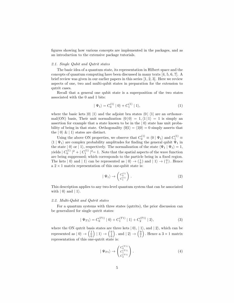
2.1. Single Qubit and Qutrit states

The basic idea of a quantum state, its representation in Hilbert space and theconcepts of quantum computing have been discussed in many texts [4, 5, 6, 7]. Abrief review was given in our earlier papers in this series [1, 2, 3]. Here we reviewaspects of one, two and multi-qubit states in preparation for the extension toqutrit cases.

Recall that a general one qubit state is a superposition of the two statesassociated with the 0 and 1 bits:

| Ψ1〉 = C(1)0 | 0〉+ C

(1)1 | 1〉, (1)

where the basic kets |0〉 |1〉 and the adjoint bra states 〈0 | 〈1| are an orthonor-mal(ON) basis, Their unit normalization 〈0 | 0〉 = 1, 〈1 | 1〉 = 1 is simply anassertion for example that a state known to be in the | 0〉 state has unit proba-bility of being in that state. Orthogonality 〈0|1〉 = 〈1|0〉 = 0 simply asserts thatthe | 0〉 & | 1〉 states are distinct.

Using the above ON properties, we observe that C(1)0 ≡ 〈0 | Ψ1〉 and C

(1)1 ≡

〈1 | Ψ1〉 are complex probability amplitudes for finding the general qubit Ψ1 inthe state | 0〉 or | 1〉, respectively. The normalization of the state 〈Ψ1 | Ψ1〉 = 1,

yields | C(1)0 |2 + | C(1)

1 |2= 1. Note that the spatial aspects of the wave functionare being suppressed; which corresponds to the particle being in a fixed region.The kets | 0〉 and | 1〉 can be represented as | 0〉 → ( 1

0 ) and | 1〉 → ( 01 ) . Hence

a 2× 1 matrix representation of this one-qubit state is:

| Ψ1〉 →(

C(1)0

C(1)1

). (2)

This description applies to any two-level quantum system that can be associatedwith | 0〉 and | 1〉.

2.2. Multi-Qubit and Qutrit states

For a quantum systems with three states (qutrits), the prior discussion canbe generalized for single qutrit states:

| ΨT1〉 = C(T1)0 | 0〉+ C

(T1)1 | 1〉+ C

(T1)2 | 2〉, (3)

where the ON qutrit basis states are three kets | 0〉, | 1〉, and | 2〉, which can be

represented as | 0〉 →(

100

)| 1〉 →

(010

). and | 2〉 →

(001

). Hence a 3× 1 matrix

representation of this one-qutrit state is:

| ΨT1〉 →

(C

(T1)0

C(T1)1

C(T1)2

). (4)

5

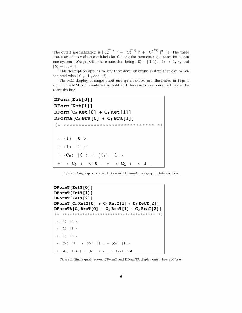
The qutrit normalization is | C(T1)0 |2 + | C(T1)

1 |2 + | C(T1)2 |2= 1. The three

states are simply alternate labels for the angular moment eigenstates for a spinone system | SMS〉, with the connection being | 0〉 →| 1, 1〉, | 1〉 →| 1, 0〉, and| 2〉 →| 1,−1〉.

This description applies to any three-level quantum system that can be as-sociated with | 0〉, | 1〉, and | 2〉.

The MM display of single qubit and qutrit states are illustrated in Figs. 1& 2. The MM commands are in bold and the results are presented below theasterisks line.

[[]]

[[]]

[ [] + []]

[ [] + []]

(* ****************************** *)

+ () | >

+ () | >

+ () | > + () | >

+ ( ) < | + ( ) < |

Figure 1: Single qubit states. DForm and DFormA display qubit kets and bras.

[[]]

[[]]

[[]]

[ [] + [] + []]

[ [] + [] + []]

(* ************************************* *)

+ () | >

+ () | >

+ () | >

+ () | > + () | > + () | >

+ () < | + () < | + () < |

Figure 2: Single qutrit states. DFormT and DFormTA display qutrit kets and bras.

6

2.2.1. Two-Qubit states

For two qubits, we have a product state | q1 q2〉 =| q1〉 | q2〉, where q1, q2 takeon the values 0 and 1. This product is called a tensor product and is symbolizedas

| q1 q2〉 =| q1〉⊗ | q2〉. (5)

In QDENSITY , the kets | 0〉, | 1〉 are invoked by the commands Ket[0] andKet[1], and the two-qubit product state by | 00〉 = AF [Ket[0]⊗Ket[0]] , where“AF” denotes array flatten 3.

The four kets | 00〉, | 01〉, | 10〉, and | 11〉 can be represented as 4×1 matrices

| 00〉 →

1000

; | 01〉 →

0100

; | 10〉 →

0010

; | 11〉 →

0001

. (6)

Hence, a 4× 1 matrix representation of the two-qubit state

| Ψ2〉 = C(2)0 | 00〉+ C

(2)1 | 01〉+ C

(2)2 | 10〉+ C

(2)3 | 11〉, (7)

is:

| Ψ2〉 →

C

(2)0

C(2)1

C(2)2

C(2)3

. (8)

Again C(2)0 ≡ 〈00 | Ψ2〉, C(2)

1 ≡ 〈01 | Ψ2〉, C(2)2 ≡ 〈10 | Ψ2〉, and C

(2)3 ≡ 〈11 | Ψ2〉,

are complex probability amplitudes for finding the two-qubit system in the states| q1 q2〉. The normalization of the state 〈Ψ2 | Ψ2〉 = 1, yields

| C(2)0 |2 + | C(2)

1 |2 + | C(2)2 |2 + | C(2)

3 |2= 1. (9)

Note that we label the amplitudes using the decimal equivalent of the bit product

q1 q2, so that for example a binary label on the amplitude C(2)10 is equivalent to

the decimal label C(2)2 .

2.2.2. Two-Qutrit states

For two qutrits, we have a product state | q1 q2〉 =| q1〉 | q2〉,where q1, q2take on the values 0, 1, and 2. This product is called a tensor product and isalso symbolized as | q1 q2〉 =| q1〉⊗ | q2〉. In QDENSITY , the kets | 0〉, | 1〉, | 2〉are invoked by the commands KetT[0],KetT[1], and KetT[2], and the productstate by | 02〉 = AF [KetT[0]⊗KetT[2]] , where “AF” denotes array flatten. The

3The command ⊗ is now included in MM as a tensor product; however, it needs to becorrected by the command AF to be in proper matrix form. Warning:There are two typesof ⊗ in MM 9-10; we now use ⊗ defined as [TensorProduct]; not as [CircleT imes]. Bestpractice is to invoke the QDENSpalette14.

7

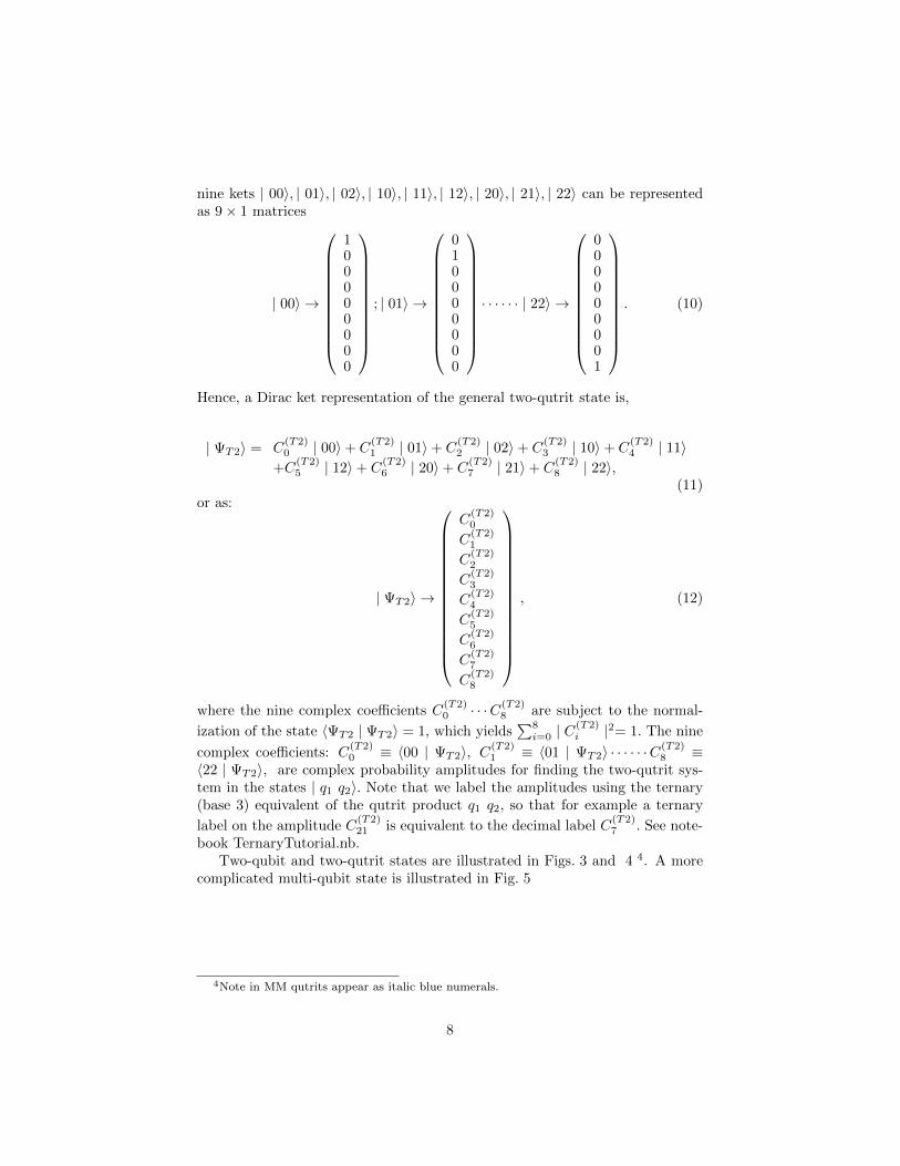
nine kets | 00〉, | 01〉, | 02〉, | 10〉, | 11〉, | 12〉, | 20〉, | 21〉, | 22〉 can be representedas 9× 1 matrices

| 00〉 →

100000000

; | 01〉 →

010000000

· · · · · · | 22〉 →

000000001

. (10)

Hence, a Dirac ket representation of the general two-qutrit state is,

| ΨT2〉 = C(T2)0 | 00〉+ C

(T2)1 | 01〉+ C

(T2)2 | 02〉+ C

(T2)3 | 10〉+ C

(T2)4 | 11〉

+C(T2)5 | 12〉+ C

(T2)6 | 20〉+ C

(T2)7 | 21〉+ C

(T2)8 | 22〉,

(11)or as:

| ΨT2〉 →

C(T2)0

C(T2)1

C(T2)2

C(T2)3

C(T2)4

C(T2)5

C(T2)6

C(T2)7

C(T2)8

, (12)

where the nine complex coefficients C(T2)0 · · ·C(T2)

8 are subject to the normal-

ization of the state 〈ΨT2 | ΨT2〉 = 1, which yields∑8

i=0 | C(T2)i |2= 1. The nine

complex coefficients: C(T2)0 ≡ 〈00 | ΨT2〉, C(T2)

1 ≡ 〈01 | ΨT2〉 · · · · · ·C(T2)8 ≡

〈22 | ΨT2〉, are complex probability amplitudes for finding the two-qutrit sys-tem in the states | q1 q2〉. Note that we label the amplitudes using the ternary(base 3) equivalent of the qutrit product q1 q2, so that for example a ternary

label on the amplitude C(T2)21 is equivalent to the decimal label C

(T2)7 . See note-

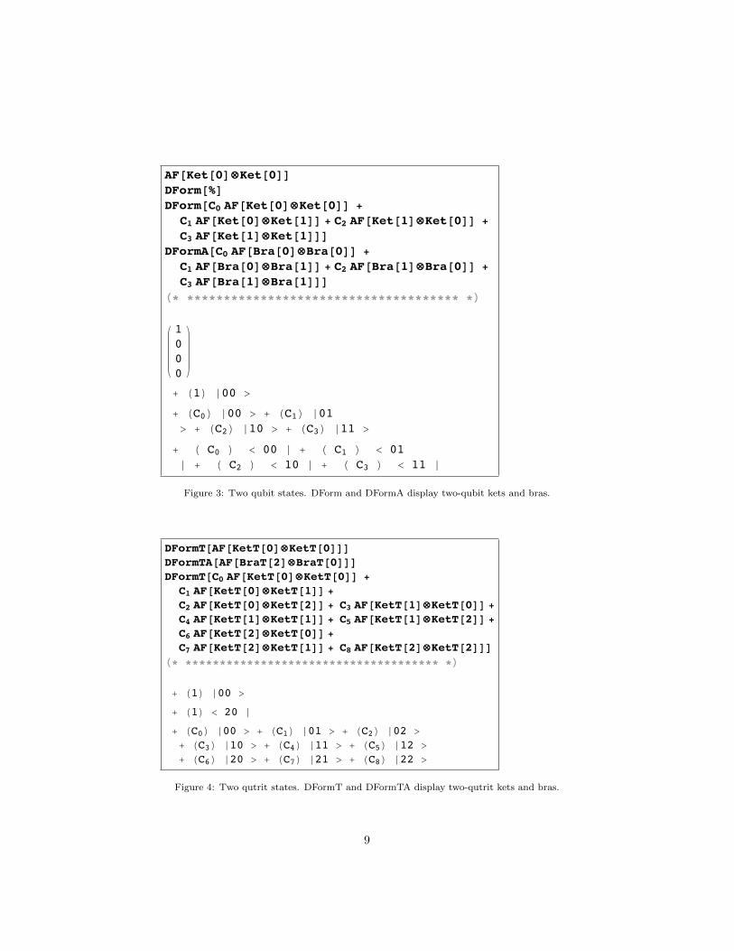
book TernaryTutorial.nb.Two-qubit and two-qutrit states are illustrated in Figs. 3 and 4 4. A more

complicated multi-qubit state is illustrated in Fig. 5

4Note in MM qutrits appear as italic blue numerals.

8

[[]⊗[]]

[%]

[ [[]⊗[]] +

[[]⊗[]] + [[]⊗[]] +

[[]⊗[]]]

[ [[]⊗[]] +

[[]⊗[]] + [[]⊗[]] +

[[]⊗[]]]

(* ************************************* *)

+ () | >

+ () | > + () |

> + () | > + () | >

+ ( ) < | + ( ) <

| + ( ) < | + ( ) < |

Figure 3: Two qubit states. DForm and DFormA display two-qubit kets and bras.

[[[]⊗[]]]

[[[]⊗[]]]

[ [[]⊗[]] +

[[]⊗[]] +

[[]⊗[]] + [[]⊗[]] +

[[]⊗[]] + [[]⊗[]] +

[[]⊗[]] +

[[]⊗[]] + [[]⊗[]]]

(* ************************************* *)

+ () | >

+ () < |

+ () | > + () | > + () | >

+ () | > + () | > + () | >

+ () | > + () | > + () | >

Figure 4: Two qutrit states. DFormT and DFormTA display two-qutrit kets and bras.

9

[ ] ⩵ [[]⊗[]⊗[]]

[[ ]]

[ [ ] +

[ ]]

(* ************************************* *)

+ () | >

+ () | > + () | >

Figure 5: Multi-qubit states using the KetV command.

2.2.3. Hybrid Qubit - Qutrit ( BT) states

Hybrid qubit-qutrit states, which we denote as BT systems, consist of bothqubits and qutrits 5. That mixture is stipulated by an array QA, such asQA= B,T,T,B, which denotes a binary ⊗ triplet ⊗ triplet⊗ binary state.A numeric array QD corresponding to that QA array is QD= 2,3,3,2 . Thedimension of the hybrid state vector is then 2nq×3nt where nq is the number ofqubits and nt the number of qutrits (triplets) in QA. In Fig. 6, a qubit-qutritQA= B,T state is displayed. A QA= B,B,T,B,T state is displayedin Fig. 7. In Fig. 8, a more complicated three-qubit,four qutrit hybrid state isshown along with the KetBT and DFormBT commands.

=

[ [[]⊗[]]]

(* ************************************* *)

+ () | >

[[]⊗[]] + [[]⊗[]]

+ [[]⊗[]] +

[[]⊗[]] + [[]⊗[]]

+ [[]⊗[]]

[ %]

(* ************************************* *)

+ () | > + () | > + () | > +

() | > + () | > + () | >

Figure 6: A hybrid qubit-qutrit state. DFormBT (DFormBTA) display hybrid BT kets (bras).Subscripts indicate if the entry is a qubit or qutrit.

5Examples of how to produce BT systems are discussed in the article [10]

10

=

[[]⊗[]⊗[]⊗[]⊗[]]

[ %]

(* ************************************* *)

+ () | >

Figure 7: A hybrid QA= B,B,T,B,T state .

= []

= / → → []

= [ ]

= [ ]

= ×

(* ************************************* *)

--

[ + ]

[ %]

(* ************************************* *)

+ () | >

Figure 8: A hybrid or Mixed Radix QA= B,T,T,B,B,T,T state.

11

3. Qubit and Qutrit Gates

In the previous section, general qubit and qutrit states were expressed assuperpositions of associated basis states. These basis states, such as |0 > & |1 >for qubits, and |0 >, |1 > & |2 > for qutrits, are used to construct multi-qubit,multi-qutrit, and hybrid states, which form a basis for the construction of generalstates for such systems. Now we turn to operators that act on such states andtheir associated operator basis. These operators are represented by N × Nmatrices where N is the dimension of the state vector. The general operatorcan be expressed as combinations of the N ×N operator basis, as discussed inthe following sections.

First, qubit (B) basis operators and gates are reviewed and then generalizedto the qutrit(T) and hybrid (BT) cases.

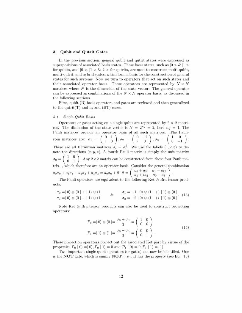
3.1. Single-Qubit Basis

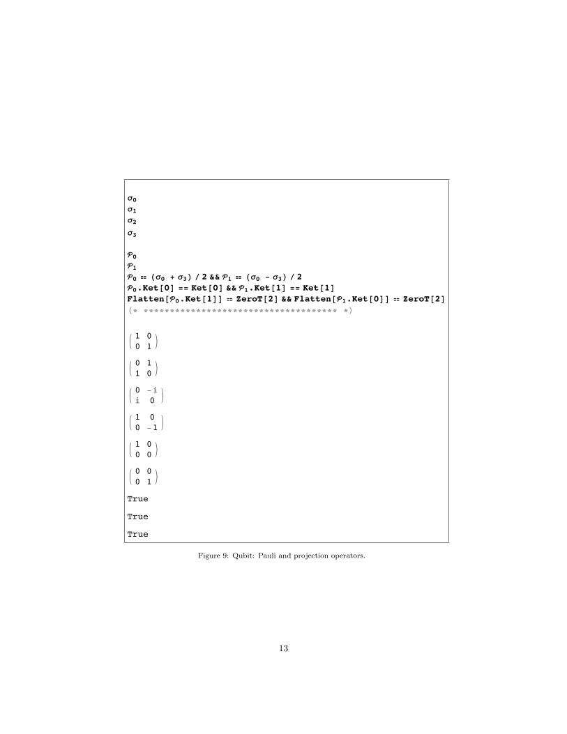
Operators or gates acting on a single qubit are represented by 2 × 2 matri-ces. The dimension of the state vector is N = 2nq = 2, here nq = 1. ThePauli matrices provide an operator basis of all such matrices. The Pauli-

spin matrices are: σ1 =

(0 11 0

), σ2 =

(0 −ii 0

), σ3 =

(1 00 −1

).

These are all Hermitian matrices σi = σ†i . We use the labels (1, 2, 3) to de-note the directions (x, y, z). A fourth Pauli matrix is simply the unit matrix:

σ0 =

(1 00 1

). Any 2×2 matrix can be constructed from these four Pauli ma-

trix. , which therefore are an operator basis. Consider the general combination

a0σ0 + a1σ1 + a2σ2 + a3σ3 = a0σ0 + ~a · ~σ =

(a0 + a3 a1 − ia2a1 + ia2 a0 − a3

).

The Pauli operators are equivalent to the following Ket ⊗ Bra tensor prod-ucts:

σ0 =| 0〉 ⊗ 〈0 | + | 1〉 ⊗ 〈1 |σ3 =| 0〉 ⊗ 〈0 | − | 1〉 ⊗ 〈1 |

&σ1 = +1 | 0〉 ⊗ 〈1 | +1 | 1〉 ⊗ 〈0 |σ2 = −i | 0〉 ⊗ 〈1 | +i | 1〉 ⊗ 〈0 |

. (13)

Note Ket ⊗ Bra tensor products can also be used to construct projectionoperators:

P0 =| 0〉 ⊗ 〈0 |= σ0 + σ32

=

(1 00 0

)P1 =| 1〉 ⊗ 〈1 |= σ0 − σ3

2=

(0 00 1

).

(14)

These projection operators project out the associated Ket part by virtue of theproperties P0 | 0〉 =| 0〉,P0 | 1〉 = 0 and P1 | 0〉 = 0,P1 | 1〉 =| 1〉.

Two important single qubit operators (or gates) can now be identified. Oneis the NOT gate, which is simply NOT = σ1. It has the property (see Eq. 13)

12

σ

σ

σ

σ

⩵ (σ + σ) / ⩵ (σ - σ) /

[] == [] [] == []

[[]] ⩵ [] [[]] ⩵ []

(* ************************************* *)

-ⅈ

ⅈ

-

Figure 9: Qubit: Pauli and projection operators.

13

NOT | 0〉 =| 1〉 and NOT | 1〉 =| 0〉. The second single qubit operator is theHadamard

H =σ1 + σ3√

2=

1√2

(1 11 −1

), (15)

which has the property H | 0〉 = |0〉+|1〉√2,H | 1〉 = |0〉−|1〉√

2.

The above steps for qubits, illustrated in Figs. 9-10, will be generalized toqutrits later.

ℋ

[ℋ []]

[ℋ []]

ℋ ⩵ (σ + σ)/[]

(* ************************************* *)

-

+ (

) | > + (

) | >

+ (

) | > + (-

) | >

Figure 10: Qubit: Hadamard operator.

3.2. Multi-Qubit Operator Basis

Consider a multi-qubit operator for nq=2. The most important one is theCNOT gate, which is defined by

CNOT = P0 ⊗ I + P1 ⊗ σ1 =

1 0 0 00 1 0 00 0 0 10 0 1 0

, (16)

where I = σ0 is the 2×2 identity matrix. The matrix above is for the case thatqubit 1 is the control and the NOT gate acts on qubit 2 only when the controlqubit 1 has the value 1. This CNOT gate produces the changes: | 00 >→| 00 >, | 01 >→| 01 >, | 10 >→| 11 > & | 11 >→| 10 > .

14

[ ]

[ ] == [⊗σ] +[⊗σ]

[ ]

[ ] ==

[(⊗ + ⊗ + ⊗)⊗σ] + [⊗⊗σ]

(* ************************************* *)

Figure 11: Qubit: CNOT and Toffoli gates.

For nq=3 the most important gate is the Toffoli gate, which is defined by

Toffoli = (P0⊗P0+P0⊗P1+P1⊗P0)⊗I+P1⊗P1⊗σ1 =

1 0 0 0 0 0 0 00 1 0 0 0 0 0 00 0 1 0 0 0 0 00 0 0 1 0 0 0 00 0 0 0 1 0 0 00 0 0 0 0 1 0 00 0 0 0 0 0 0 10 0 0 0 0 0 1 0

.

(17)This is for the case that qubits 1 & 2 are the control qubits and the NOT

gate acts on qubit 3 only when the control qubits both have the value 1.This qubit gate is generated as shown in Fig. 11; it will be generalized to

qutrits later.

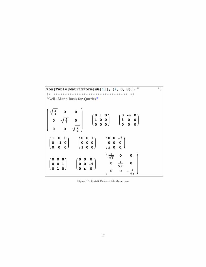
3.3. Single-Qutrit Basis and Gates

The operator basis for qutrits consists of nine matrices; there are severalpossible choices for the 9 operators. One choice uses the unit matrix plus thethree spin-one spin matrices, along with a rank 2 Cartesian tensor. Another

15

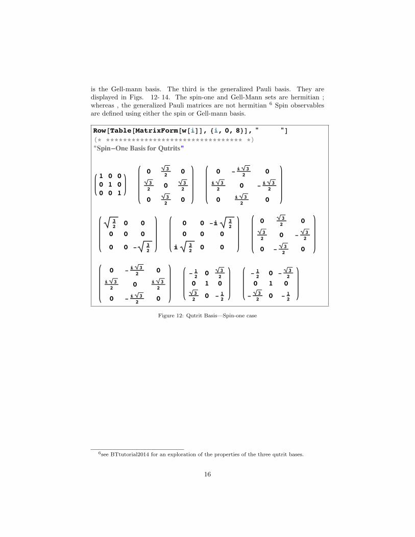
is the Gell-mann basis. The third is the generalized Pauli basis. They aredisplayed in Figs. 12- 14. The spin-one and Gell-Mann sets are hermitian ;whereas , the generalized Pauli matrices are not hermitian 6 Spin observablesare defined using either the spin or Gell-mann basis.

[[[[]] ] ]

(* ******************************** *)

-

-ⅈ

ⅈ

-ⅈ

ⅈ

-

-ⅈ

ⅈ

-

-

-ⅈ

ⅈ

ⅈ

-ⅈ

-

-

-

-

-

-

Figure 12: Qutrit Basis—Spin-one case

6see BTtutorial2014 for an exploration of the properties of the three qutrit bases.

16

[[[[]] ] ]

(* ******************************** *)

-

-ⅈ ⅈ

-

-ⅈ

ⅈ

-ⅈ

ⅈ

-

Figure 13: Qutrit Basis—Gell-Mann case

17

[[[[]] ] ]

(* ******************************** *)

ⅇⅈπ

ⅇ-ⅈπ

ⅇⅈπ

ⅇ-ⅈπ

ⅇⅈπ

ⅇ-ⅈπ

ⅇ-ⅈπ

ⅇⅈπ

ⅇ-ⅈπ

ⅇⅈπ

ⅇ-ⅈπ

ⅇⅈπ

Figure 14: Qutrit Basis—Generalized Pauli

Qutrit gates are often defined using the Pauli basis. For example, one definesa qutrit NOT gate as the generalized X operator, which is given in Fig. 15, wherewe see that X | i〉 =| Mod[i+ 1, 3]〉. A qutrit Hadamard acts on a single qutritas shown in Fig. 16. The qutrit Hadamard generates three orthonormal linearcombinations of three basic qutrit kets, incorporating a phase factor ξ(k) =

exp−2πik

3 .

= []

(* ****** **************** *)

[ []]

[ []]

[ []]

+ () | >

+ () | >

+ () | >

Figure 15: Qutrit Basis—NOT gate

18

ℋ

(* ********************** *)

ⅇ-ⅈπ

ⅇⅈπ

ⅇⅈπ

ⅇ-ⅈπ

(* ********************** *)

[ ℋ[]]

[ ℋ[]]

[ ℋ[]]

+ (

) | > + (

) | > + (

) | >

+ (

) | > + (

ⅇ- ⅈ π

) | > + (

ⅇ ⅈ π

) | >

+ (

) | > + (

ⅇ ⅈ π

) | > + (

ⅇ- ⅈ π

) | >

Figure 16: Qutrit Basis—the qutrit Hadamard HT .

3.4. Multi-Qutrit Basis and Gates

In the previous section, the single qutrit states and gates were presented.Now we extend that discussion to two or more qutrits. Later, we will discusshybrid cases wherein a mixture of qubits and qutrits are stipulated. The tutorialGatesQudits2015 explores these topics in great detail.

To generate an operator basis for two qutrits, we form a tensor productw(i)⊗ w(i), as shown in Fig. 17. An example of a two-qutrit operator is twoHadamards acting on both qutrits HT ⊗HT , as shown in Fig. 18.

19

-

[ ] ⩵ [[]⊗ []]

[ ] ⩵ [[]⊗[]⊗[]⊗ []]

[[]⊗ []]

ⅈ

ⅈ

-ⅈ

ⅈ

ⅈ

-ⅈ

-

ⅈ

-

ⅈ

-

ⅈ

ⅈ

ⅈ

- ⅈ

-

ⅈ

-

ⅈ

-

ⅈ

ⅈ

ⅈ

-ⅈ

ⅈ

ⅈ

Figure 17: Multi-qutrit basis and the SPT command

20

ℋ

ℋ = [ℋ ⊗ℋ]

ℋ[[]⊗[]]

[ %]

ℋ[[]⊗[]]

[ %]

ⅇ-ⅈπ

ⅇ

ⅈπ

ⅇ

ⅈπ

ⅇ-ⅈπ

+ (

) | > + (

) | > + (

) | > + (

) | > + (

)

| > + (

) | > + (

) | > + (

) | > + (

) | >

+ (

) | > + (

ⅇⅈπ

) | > + (

ⅇ-ⅈπ

) | > + (

) | > + (

ⅇⅈπ

) |

> + (

ⅇ-ⅈπ

) | > + (

) | > + (

ⅇⅈπ

) | > + (

ⅇ-ⅈπ

) | >

Figure 18: Two qutrit Hadamards on two qutrits

Another two-qutrit operator can be defined using the same procedure dis-cussed earlier for the CNOT two-qubit gate. First we need the qutrit projectionoperators:

PT0 =| 0〉 ⊗ 〈0 |=

(1 0 00 0 00 0 0

)

PT1 =| 1〉 ⊗ 〈1 |=

(0 0 00 1 00 0 0

)

PT2 =| 2〉 ⊗ 〈2 |=

(0 0 00 0 00 0 1

).

(18)

These projection operators project out the associated qutrit kets. The sum ofthese three projection operators equals a 3× 3 unit matrix I3.

Now, we can define a controlled-not gate for qutrits in a variety of ways.The first uses qutrit 1 as the control, with the qutrit Pauli NOT gate X=wP[1]acting on qutrit 2 as follows:

CNOT1 = PT0 ⊗ I3 + PT

1 ⊗X + PT2 ⊗X ·X. (19)

Since X is not Hermitian CNOT1† 6= CNOT1, in contrast to the qubit casewhere σ1 is Hermitian.

The second uses qutrit 2 as the control, with the qutrit NOT gate X actingon qutrit 1.

CNOT2 = I3 ⊗ PT0 + X⊗ PT

1 + X ·X⊗ PT2 . (20)

21

The explicit form for CNOT1 is

CNOT1 =

1 0 0 0 0 0 0 0 00 1 0 0 0 0 0 0 00 0 1 0 0 0 0 0 00 0 0 0 0 1 0 0 00 0 0 1 0 0 0 0 00 0 0 0 1 0 0 0 00 0 0 0 0 0 0 1 00 0 0 0 0 0 0 0 10 0 0 0 0 0 1 0 0

,

and for CNOT2

CNOT2 =

1 0 0 0 0 0 0 0 00 0 0 0 0 0 0 1 00 0 0 0 0 1 0 0 00 0 0 1 0 0 0 0 00 1 0 0 0 0 0 0 00 0 0 0 0 0 0 0 10 0 0 0 0 0 1 0 00 0 0 0 1 0 0 0 00 0 1 0 0 0 0 0 0

.

Control-Z, and Control-Y Gates can also be constructed using the qutritPauli Y=wP[2] and & Z=wP[3] gates

CZT1 = PT0 ⊗ I3 + PT

1 ⊗ Z + PT2 ⊗ Z · Z

CZT2 = I3 ⊗ PT0 + Z⊗ PT

1 + Z · Z⊗ PT2

CY T1 = PT0 ⊗ I3 + PT

1 ⊗Y + PT2 ⊗Y ·Y

CY T2 = I3 ⊗ PT0 + Y ⊗ PT

1 + Y · Y ⊗ PT2 .

(21)

The above CNOT1 & CNOT2 gates do not provide a swap gate followingthe qubit pattern. To produce a qutrit swap gate another pair of CNOT gatesare introduced. [8, 9], as shown in Fig. 19- 21. This modified swap also workswhen two qutrit operators are used within a multi-qutrit system, see later.

CNOTH1 = (I3 ⊗HT †) · CZT1 · (I3 ⊗HT †)CNOTH2 = (HT † ⊗ I3) · CZT2 · (HT † ⊗ I3).

(22)

Here HT is the qutrit Hadamard.

22

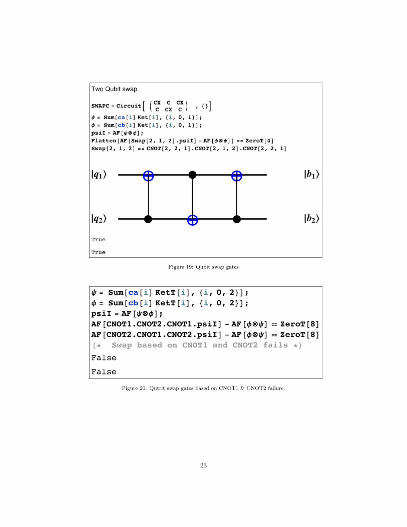
Two Qubit swap

=

ψ = [[] [] ]

ϕ = [[] [] ]

= [ψ⊗ϕ]

[[[ ]] - [ϕ⊗ψ]] == []

[ ] == [ ][ ][ ]

|⟩

|⟩

⊕ ⊕

⊕

|⟩

|⟩

Figure 19: Qubit swap gates

ψ = [[] [] ]

ϕ = [[] [] ]

= [ψ⊗ϕ]

[] - [ϕ⊗ψ] ⩵ []

[] - [ϕ⊗ψ] ⩵ []

(* *)

Figure 20: Qutrit swap gates based on CNOT1 & CNOT2 failure.

23

ψ = [[] [] ]

[ψ]

ϕ = [[] [] ]

[ϕ]

= [ψ⊗ϕ]

= [ϕ⊗ψ]

[] ⩵

[] ⩵

(* ************************************* *)

+ ([]) | > + ([]) | > + ([]) | >

+ ([]) | > + ([]) | > + ([]) | >

Figure 21: Qutrit swap gates based on CNOTH success

3.5. Qubit-Qutrit Operators

For a hybrid system consisting of one qubit and one qutrit, the single qubitand single qutrit operators are as defined earlier. The two-body BT or TBcontrol operators can be defined in various ways. For example, CNOTBT1 withqubit 1 as control can be stipulated as 7

CNOTBT1 = P0 ⊗ I3 + P1 ⊗X,

whereas, for CNOTTB1 with qutrit 1 as control and qubit 2 acted on by σ1 canbe defined in several ways. One way is

CNOTTB1 = PT0 ⊗ I2 + PT

1 ⊗ σ1 + PT2 ⊗ I2,

Another way is

CNOTTB1 = PT0 ⊗ I2 + PT

1 ⊗ σ1 + PT2 ⊗ σ1.

Based on these examples, the user can explore other such qubit-qutrit operators.

7I3 denotes a unit 3× 3 matrix and I2 denotes a unit 2× 2 matrix.

24

3.6. General Operators

3.6.1. General Qubit Operators

In the pure multi-qubit case, the general form of multi-qubit operators areprovided by several QDensity commands. For example, had[n, i ] is an oper-ator for n qubits with a single Hadamard acting on qubit “i;” Had[n,Q] is ann-qubit operator with Hadamards acting on all members of the set Q=q1,q2,... of length n, where if qi is set to 1 that qubit is acted on by a Hadamard, whereasa value of 0 specifies no action on that qubit. For example,Had[3,1,0,1]has Hadamards acting on qubits 1 and 3 for a three qubit system. To get aHadamard acting on all qubits, include all qubits in Q, e.g., use Q=1,1,1,.....HALL[n]=Had[n,1,1,1....] is also provided where the array Q of 1’s haslength n to include all the qubits. See Fig. 22.

A similar setup is included in QDensity for projection operators; proj[n,i,a]is an n-qubit operator, which yields a projection operator P0 for a=0 or P1

for a=1 acting on qubit “i.” Also, an n-qubit projection operator PJ[n,Q,A]is defined which acts on set q1,q2,... of the n qubits along with an array A=a1.... which stipulates if the projection on the qubit is either zero or one;if ai is not equal to zero or one then the unit operator I=s[0] is taken for the ithqubit . Thus, one can build an operator of the type: I⊗P0⊗P1⊗I⊗P0⊗P1⊗I,which asks if the qubits 2,3,5,6 have the values 0101 .

3.6.2. General Qutrit Operators

Similar commands are now available for pure qutrit systems Fig. 23. . Thecommand SPT[n,Q] for n qutrits produces a spin basis tensor product withcomponents stipulated by the array Q; for example, SPT[3,2,1,2] yields thespin-basis tensor product w[2]⊗ w[1] ⊗ w[2]. To extend this procedure to qutritHadamards and projection operators, we set the w[i > 8] matrices as follows:w[10] =HT , w[11] =X , w[12+i] =PT i, w[16] =X.X , w[33] =Z , w[34] =Z.Z. Here X and Z are the Pauli qutrit operators. Using these settings we see inFig. 23 that SPT[n,Q] for n=3, Q=10,11,12 yields HT ⊗X⊗PT 0. A moregeneral command SPBTA[n,QA,Q] will be discussed next.

3.6.3. General BT Hybrid Operators

For hybrid (mixed radix, BT) systems we have a mixture of qubits andqutrits as stipulated by the array QA. Examples of general operators for suchBT systems are presented in Figs. 23- 24. For example, we see that a systemwith QA= B,T,B,T (i.e. a qubit×qutrit×qubit×qutrit system) with a NOToperator on the qubits 1 and 3, a Hadamard on the qutrit 3 and a projectionoperator on the qutrit 4 is generated by the command SPBTA[4,QA,Q] , withQ= 1,10,,11,12. Here s[11] is equal to s[1]=NOT. Special cases of pure B orpure T systems can be invoked and seen to be equivalent to earlier SP and SPTforms.

As a further generalization of earlier commands for general operators, see theexamples in Fig. 25. There we display commands HadBT, hadBT, OneOpBT

25

and TwoOpBT. These are used in the BTSystems tutorial, along with Three-OpBT, to construct generalized BT operators such as control-not, swap, control-z, TofolliBT, etc gates.

Another method to generate general operators for BT systems, is to applythe one and two body operators OpBT1, OpBT2 or OpBT3 to the full set ofbasis vectors, as is included in the commands BTOp1 and BTOp2 (see thetutorials).

With these tools any general BT operation can be constructed and used tostudy such systems. Cases of random B,T and BT states and density matricesare also incorporated into the package as illustrated in the associated tutorials.

[[ ][[]⊗[]]]

(* ************************************************ *)

+ () | > + (

) | > + (

) | > + (

) | >

[[ ][[]⊗[]⊗[]]]

[ ] == [ℋ ⊗ℋ ⊗ℋ]

[ ] == [ℋ ⊗ℋ ⊗ℋ ⊗ℋ]

(* ************************************************* *)

+ (

) | > + (

) | > + (

) | > + (

) | > +

(

) | > + (

) | > + (

) | > + (

) | >

Figure 22: General qubit operators, Hadamard example.

26

ℋ

ⅇ-ⅈπ

ⅇ

ⅈπ

ⅇ

ⅈπ

ⅇ-ⅈπ

[ ] == [[]⊗[]⊗[]]

[ ] == [ℋ⊗⊗] ==

[ ]

[] ⩵ ℋ [] ⩵ [] == [] == [] == [] ⩵ [] ⩵ ℤ [] ⩵ [] ⩵ ℤ [] ⩵ ℤℤ

[ ] == [ℋ⊗⊗] ==

[ ]

[ [ ] [ ]] ==

[ℋ⊗ℋ⊗ℋ⊗ℋ⊗ℋ]

[ [ ] [ ]] ==

[ ⊗ ⊗ ⊗ ⊗]

Figure 23: General qutrit operator examples

27

[ ] == [[]⊗ ℋ]

[ ] == [ℋ⊗ ℋ]

[ ] == [ℋ ⊗ℋ]

[ ] == [[]⊗[]⊗[]]

[ ] == [ℋ⊗⊗]

[ ] == [[]⊗ ℋ]

[ ] == [ℋ⊗ ℋ]

[ ] == [[]⊗ℋ⊗[]⊗]

[] ⩵ ℋ ⩵ [] [] == ⩵ [] [] == [] ⩵ []

[ [ ]] ==

ℋ ⊗ℋ ⊗ℋ⊗ℋ⊗ℋ

[ [ ]] == [ ⊗ ⊗ ⊗ ⊗]

Figure 24: General hybrid BT operator examples

[ ] ⩵ [ℋ ⊗ℋ]

[ ] ⩵ [ℋ ⊗[]⊗ℋ] == [ ]

[ ] ⩵ [ℋ ⊗[]⊗ℋ] == [ ]

= = = []

[ ] == [[] ⊗ℋ⊗[]]

[ ] ⩵ [[]⊗ []⊗ []⊗ []]

[ ] == [[]⊗ []⊗ []]

[ ] == [[]⊗ []⊗ []]

[ ] ⩵ [[]⊗ []⊗ []⊗ []]

[ ] ⩵ [[]⊗ []⊗ []⊗ []] ==

[[]⊗ []⊗ ℋ⊗ []]

[ ] ⩵ [[]⊗ []⊗ []⊗ []] ⩵

[[]⊗ []⊗ []⊗ ℋ]

[ ] == [ []⊗ []]

[ ] == [ []⊗ []]

[ ] == [ []⊗ []]

[ ] == [ []⊗ []⊗ []]

[ ] == [[]⊗ []⊗ []⊗ []]

[ ] == [ []⊗ []]

Figure 25: Additional hybrid BT operator examples

28

4. Entanglement

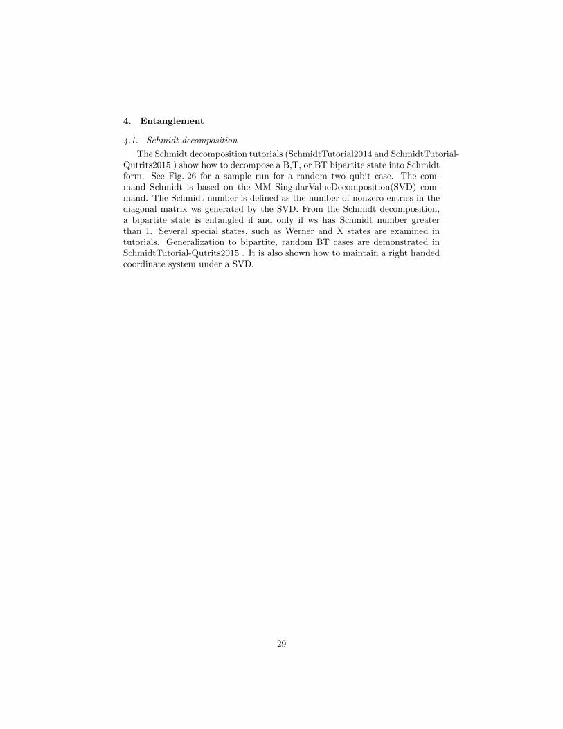
4.1. Schmidt decomposition

The Schmidt decomposition tutorials (SchmidtTutorial2014 and SchmidtTutorial-Qutrits2015 ) show how to decompose a B,T, or BT bipartite state into Schmidtform. See Fig. 26 for a sample run for a random two qubit case. The com-mand Schmidt is based on the MM SingularValueDecomposition(SVD) com-mand. The Schmidt number is defined as the number of nonzero entries in thediagonal matrix ws generated by the SVD. From the Schmidt decomposition,a bipartite state is entangled if and only if ws has Schmidt number greaterthan 1. Several special states, such as Werner and X states are examined intutorials. Generalization to bipartite, random BT cases are demonstrated inSchmidtTutorial-Qutrits2015 . It is also shown how to maintain a right handedcoordinate system under a SVD.

29

= []

[%]

[]

[ϕ= ϕ]

[ϕ= ϕ]

[ϕ= ϕ]

[ϕ= ϕ]

[= []]

[= ]

+ ( + ⅈ) | > + (- - ⅈ) | >

+ (- + ⅈ) | > + ( + ⅈ) | >

ϕ= + (-) | > + ( - ⅈ) | >

ϕ= + (-) | > + (- + ⅈ) | >

ϕ= + (- - ⅈ) | > + ( + ⅈ) | >

ϕ= + (- - ⅈ) | > + (- - ⅈ) | >

=

=

== []

- + ⅈ - + ⅈ

- ⅈ - + ⅈ

- - ⅈ + ⅈ

- - ⅈ - - ⅈ

+ ⅈ - - ⅈ

- + ⅈ + ⅈ

Figure 26: Schmidt decomposition for a random 2 qubit state m.

30

4.2. Entropy, mutual information, Quantum Discord

=

Ω = []

= [Ω]

= [[Ω]]

[ → → → → []]

[[ΩΩ]]

[] == [[[]] ] == [Ω] ⩵

== [[[]] ] ⩵ [Ω] == [[ΩΩ]]

= [Ω]

0 5 10 15 20 25 30 35

0.02

0.04

0.06

0.08

0.10

Ω = [ Ω]

[[%]] ⩵

Ω = [ Ω]

[[%]] ⩵

= [Ω]

= [Ω]

= + -

[Ω] [Ω] == [Ω]

Figure 27: Mutual Information example for a random BT density matrix Ω.

31

Ω = ℐ = [ Ω ] ℐ = [ Ω ][= = = ℐ= ℐ]

[= = ][= = ]

= = = ℐ=

= =

= =

= [[ ] ] = [[ ] ]

[ ]

Figure 28: Discord example. Here Ω is a random 2-qubit density matrix, I is the mutualinformation, CA the classical and QA the discord. Surfaces for classical search are alsoshown.

[ Ω_ / [Ω] _ _] =

[ ℐ ρ

=

= Ω = [ ] = [ ]

= [] = [] = []

ℐ = [ + - ]

[_] = [[ [θ] [ϕ] [θ] [ϕ] [θ]]

ϕ θ ∈ ]

= [ == [[σ ]⊗[]] [[]⊗[σ ]]]

= [ == ]

[_] = [[ ] ϕ θ ∈ ]

[_ _ _] = [[] / θ -> ϕ -> ]

ρ[_] = [ [ ] ϕ θ ∈ ]

[_ _ _] = [ρ[] / [] / θ -> ϕ -> ]

[]

[_ _] = [ [ ] * [[ ]]

]

[_ _] = [ * / () * / ]

= [ [ ] [ ]]

= []

= [ == [] - [] - ]

= ℐ -

ℐ ]

Figure 29: The module Discord[ρ, Ic, np] = I[ρ] − C[ρ], where C is the classical evaluationof the conditional entropy < J >C . Note Ic selects the discord case JA or JB and npstipulates the space used in the requisite minimization and in the plot. Discord provides theoutput array (SA, SB, SAB, I, C,D, plot).

32

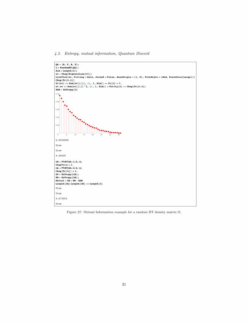
The entropy command EnTropy 8 is used to evaluate the von Neumannentropy from the real, positive eigenvalues of a density matrix ρ, EnTropy[ρ] =−Tr[ρ ln ρ]. The density matrix can be generated from a random density matrixcommand, (RandomQubit1, RandomQubit2, RandomQubitN, RandomQutrit,or RandomBT), or from a state Ψ just by the command ρ[Ψ]. Density matrixconstruction for BT systems is explored in the notebook DensityMatrixTutorial.

4.2.1. Partial Trace

Once the entropy is determined from a given density matrix, the Partial-Trace and PartialTraceBT commands can be used to determine the sub-systemdensity matrices and their associated entropy, and thus the mutual informa-tion is specified. For example, using PartialTraceBT for a RandomBT den-sity matrix, the mutual information I ≡ SA + SB − SAB is determined inFig. 27. Here SAB = EnTropy[ρ], SA = EnTropy[ρA], SB = EnTropy[ρB ],where SAB is the full system entropy, and SA, SB are the subsystem en-tropies. The subsystem density matrices are: ρA = TrB [ρ] = PTr[2, ρ] andρB = TrA[ρ] = PTr[1, ρ]

4.2.2. Discord

The quantum discord involves using two forms for the mutual informationthat are equal for a classical system, but differ for a quantum system. Theidea of quantum discord was introduced in references [11, 12], where Ollivierand Zurek[11] describes it as “ Two classically identical expressions for themutual information generally differ when the systems involved are quantum.This difference defines the quantum discord. It can be used as a measure of thequantumness of correlations.” The discord indicates that quantum effects, butnot necessarily quantum entanglement, exist in the system,.

The two quantum relations for the mutual information are

I = S[ρA] + S[ρB ]− S[ρ] (23)

and

JA = S[ρB ]− S[B|A],

or

JB = S[ρA]− S[A|B],

where S[ρA] and S[ρB ] are the von Neumann entropies for the A and B sub-systems, respectively. That is : S[ρA] = EnTropy[ρA], S[ρB ] = EnTropy[ρB ],where ρA = TrB [ρ], ρB = TrA[ρ], and S[A,B] = EnTropy[ρ]. Here S[A,B] isthe joint entropy. The quantities S[A|B] = S[ρA|ρA], S[B|A] = S[ρB |ρA] de-note quantum conditional entropies. Note that for the case that A and B areseparate and unconnected systems, the density matrix is a product ρ = ρA⊗ρBand then the mutual information I = 0.

8We use the command EnTropy to obtain the von Neumann entropy, The MM commandEntropy is not the same quantity.

33

For a classical system, classical renditions of the two expressions for themutual information I,JA yield identical results,; however, for the quantumcase I 6= JA. The difference between the two results are used to define thediscord

DA(ρ) = I − JA (24)

and

DB(ρ) = I − JB.

In general, DA(ρ) 6= DB(ρ). The problem now is how to evaluate JA and JA.The quantities JA and JA represent ”the part of the correlations that canbe attributed to classical correlations and varies in dependence on the choseneigenbasis; therefore, in order for the quantum discord to reflect the purelynonclassical correlations independently of basis, it is necessary that J first bemaximized over the set of all possible projective measurements onto the eigen-basis.” [13] That process, which entails an evaluation of the conditional entropyusing a classical limit method, is incorporated into Qdensity as shown in Fig.29.

Sample cases are shown in the three discord notebooks.

4.3. Partial Transposition

Examples of partial transposition are shown in the tutorial ” PartialTrans-pose Tutorial.” In this package, the partial transpose is obtained by expandingthe density matrix in the computational (Pauli tensor product) basis. Then forthe stipulated subsystem, the subsystem Pauli matrices are transposed, and thenthe transposed density matrix is reconstructed. The only subsystem operatorsthat are affected are those involving the y-component Pauli operators. This pro-cedure is encoded in the module PartialTranspose[BL,ρ] , where BL stipulatesthe subsystem and ,ρ is the original density matrix. This procedure is gener-alized to hybrid (BT) systems by the module PartialTransposeBT[QA,BL,ρ],BL again stipulates the subsystem and now the array QA gives the BT mix-ture. Examples and tests are provided in the PartialTransposeTutorial and alsoused to demonstrate the Peres−Horodecki [14] criterion for separable densitymatrices in tutorials ”.

Calculation and display of Entropy, mutual information and quantum dis-cord are also provided in “ PartialTranspose Tutorial.”

4.4. Bell’s theorem

In the Bell theorem and Bell Correlations2015 notebooks, sample cases ofBell’s theorem are examined using this package. For discussion, see : [6, 7, 15,16, 17]

34

5. Other new aspects

5.1. QC algorithms & Simulations

Updates of various QC algorithms [18, 19, 20] are provided in Teleporta-tion2014, Grover2014, Shor2014, QFT2014 and Cluster2014. A sample of tele-portation of a qubit is contained in TeleportationBT, Studies of random states,random density matrices, Werner [21] states, GHZ [22] states and X [23] statesare presented in various notebooks included with this package in many caseswith qutrit or hybrid system examples (see the appendix). A preliminary studyof concurrence is present in the notebooks ConcurrenceTutorial and Concur-renceTutorialBT [24, 25]

6. Future Plans: Parallel & Cuda versions

This update and extension provides many basic tools for studying the ef-ficacy of quantum computers. Some of the cases that are not included hereinclude: (1) quantum error correctionr [26], (2) dynamical evolution of gates,(3) density matrix dynamics including entropy constraints,( 4) solutions of dif-ferential equations, (5) single and multiple photon qubit states (6) QuantumTomography. Preliminary versions of these case are available, but not includedin the present release. The applications will hopefully improve, increase, andbroaden with time, perhaps by interested users.

The hope is to improve and extend this package, by future application ofMPI parallel methods to enable faster and larger system studies. Use of theGPU processor for parallel computation is also a future goal, once the highlatency problem for large system tensor product formation is solved. A webpage presentation of this package is available and questions, suggestions forfuture developments, and comments, are welcome, so that these packages canbe further improved. Do not hesitate to contact the author for help.

Acknowledgments

The author is very appreciative of the help provided by his collaboratorDr. Bruno Julia-Dıaz, who was one of the original developers of this project.Questions and comments provided by Dr. Kapil K. Sharma are also very muchappreciated; he stimulated the extensions to hybrid systems, partial transposi-tion, and to quantum discord. My interest in quantum tomography was greatlyenhanced by communications with Dr. Victor Volkov. Earlier versions of thisproject were supported by the National Science Foundation.

35

References

[1] Bruno Julia-Dıaz, Joseph M. Burdis and Frank Tabakin, “QDENSITY - AMathematica Quantum Computer simulation,” Comp. Phys. Comm., 174(2006) 914-934. Also see: Comp. Phys. Comm.,180, (2009) 474.

[2] Frank Tabakin and Bruno Julia-Dıaz, “QCWAVE A Mathematica quan-tum computer simulation update,” Comp. Phys. Comm., 182, (2011)1693.

[3] Frank Tabakin and Bruno Julia-Dıaz, “QCMPI: A parallel environment forquantum computing”, Comp. Phys. Comm., 180 (2009) 948-964.

[4] P. A. M. Dirac, “The Principles of Quantum Mechanics”, Oxford UniversityPress, USA 4th ed. ISBN: 0198520115.

[5] Albert Messiah, “Quantum Mechanics” , Dover Publications , ISBN :0486409244.

[6] Michael A. Nielsen and Isaac I. Chuang, “Quantum Computation andQuantum Information”, Cambridge University Press (2000).

[7] John Preskill, “Lecture Notes on quantum information and computation”,http://www.theory.caltech.edu/people/preskill/ph229/.

[8] C. M. Wilmott and P. R. Wild, Int. J. Quantum Inform. 10, 1250034 (2012).

[9] Juan Carlos Garcia-Escartin, Pedro Chamorro-Posada,”A SWAP gate forqudits,” Quantum Information Processing,Vol .12,(2013).

[10] Peter B R Nisbet-Jones, Jerome Dilley, Annemarie Holleczek, Oliver Barterand Axel Kuhn, “Photonic qubits, qutrits and ququads accurately preparedand delivered on demand,” New Journal of Physics 15 (2013) 053007.

[11] H. Ollivier and W. H. Zurek, Quantum discord: A measure of the quan-tumness of correlations, Phys. Rev. Lett. 88, 017901 (2002).

[12] L. Henderson and V. Vedral: Classical, quantum and total correlations,Journal of Physics A 34, 6899 (2001).

[13] https://en.wikipedia.org/wiki/

[14] Asher Peres, Separability Criterion for Density Matrices, Phys. Rev. Lett.77, 14131415 (1996) and Michal Horodecki, Pawel Horodecki, RyszardHorodecki, Separability of Mixed States: Necessary and Sufficient Con-ditions, Physics Letters A 223, 1-8 (1996).

[15] Bell, John (1964). ”On the Einstein Podolsky Rosen Paradox”. Physics 1(3): 195200.

[16] JS Bell (2004), Speakable and Unspeakable in Quantum Mechanics: Cam-bridge University Press. 2nd Edition(2004) ISBN: 9780521523387.

36

[17] http://www.lecture-notes.co.uk/susskind/quantum-entanglements/lecture-5/violation-of-bells-theorem/ .

[18] C. H. Bennett, G. Brassard, C. Crepeau, R. Jozsa, A. Peres, and W. K.Wootters, Phys. Rev. Lett. 70, 1895-1899 (1993).

[19] Peter W. Shor, SIAM J. Comput. 26 (5): 1484 (1997).

[20] L. K. Grover, Phys. Rev. Lett. 79, 325-328 (1997).

[21] Reinhard F. Werner ,Physical Review A 40 (8) 42774281.

[22] Daniel M. Greenberger, Michael A. Horne, Anton Zeilinger:, ”Bell’s the-orem, Quantum Theory, and Conceptions of the Universe,” pp. 73-76,Kluwer Academics, Dordrecht, The Netherlands (1989).

[23] Sai Vinjanampathy and A. R. P. Rau, Phys. Rev. A 82, 032336 (2010).

[24] W. K. Wootters, ”Entanglement of Formation and Concurrence,” QuantumInformation and Computation 1, 27 (2001) and W. K. Wootters,Phys.Rev.Letters 80,2245 (1998).

[25] E. Gerjuoy Phys. Rev. A 67, 052308 ( 2003).

[26] D. Gottesman, “A Theory of Fault-Tolerant Quantum Computation,”Phys. Rev. A 57, 127-137 (1998).

37

A. Tutorials

The following tutorials, workbooks and algorithms are part of the packageand should aid the user in generating their own examples. Guidance for instal-lation is provided in the notebook INSTALL. Email tabakin@pitt.edu for thepackages and for these and additional tutorials.

1. BTGates2. BTtutorial20143. Bell Correlations20154. Belltheorem5. CircuitTutorial20146. CircuitTutorialBT20157. Cluster20148. ConcurrenceTutorial9. ConcurrenceTutorial2

10. ConcurrenceTutorial311. ConcurrenceTutorialBT12. DensityMatrixTutorial13. Discord-Tests 201514. DiscordTutorial201515. Entanglement201416. EntropyTutorial201517. FunctionsTour201418. GatesQudits201519. Grover201420. HybridGates21. INSTALL22. Measurement23. PartialTransposeTutorial24. QCwaveTutorial201425. QFT201426. Quantum EntropyTutorial201427. Qutrit operators28. RandomObs29. SchmidtTutorial-Qutrits201530. SchmidtTutorial201431. Shor201432. Teleportation201433. TeleportationQutrit34. TernaryTutorial35. Tutorial201436. TutorialTP37. WernerStates201438. WorkBookPartnerBT39. XState Tutorial 201540. XState Tutorial

38