Mathematica Tutorial: Notebooks And Documents - Wolfram Research

Wolfram Mathematica ® Tutorial Collection

NOTEBOOKS AND DOCUMENTS

For use with Wolfram Mathematica® 7.0 and later.

For the latest updates and corrections to this manual: visit reference.wolfram.com

For information on additional copies of this documentation: visit the Customer Service website at www.wolfram.com/services/customerservice or email Customer Service at [email protected]

Comments on this manual are welcomed at: [email protected]

Printed in the United States of America.

15 14 13 12 11 10 9 8 7 6 5 4 3 2

©2008 Wolfram Research, Inc.

All rights reserved. No part of this document may be reproduced or transmitted, in any form or by any means, electronic, mechanical, photocopying, recording or otherwise, without the prior written permission of the copyright holder.

Wolfram Research is the holder of the copyright to the Wolfram Mathematica software system ("Software") described in this document, including without limitation such aspects of the system as its code, structure, sequence, organization, “look and feel,” programming language, and compilation of command names. Use of the Software unless pursuant to the terms of a license granted by Wolfram Research or as otherwise authorized by law is an infringement of the copyright.

Wolfram Research, Inc. and Wolfram Media, Inc. ("Wolfram") make no representations, express, statutory, or implied, with respect to the Software (or any aspect thereof), including, without limitation, any implied warranties of merchantability, interoperability, or fitness for a particular purpose, all of which are expressly disclaimed. Wolfram does not warrant that the functions of the Software will meet your requirements or that the operation of the Software will be uninterrupted or error free. As such, Wolfram does not recommend the use of the software described in this document for applications in which errors or omissions could threaten life, injury or significant loss.

Mathematica, MathLink, and MathSource are registered trademarks of Wolfram Research, Inc. J/Link, MathLM, .NET/Link, and webMathematica are trademarks of Wolfram Research, Inc. Windows is a registered trademark of Microsoft Corporation in the United States and other countries. Macintosh is a registered trademark of Apple Computer, Inc. All other trademarks used herein are the property of their respective owners. Mathematica is not associated with Mathematica Policy Research, Inc.

Contents

Notebook InterfaceNotebook Interfaces . . . . . . . . . . . . . . . . . . . . . . . . . . . . . . . . . . . . . . . . . . . . . . . . . . . . . . . . . . . . 1

Doing Computations in Notebooks . . . . . . . . . . . . . . . . . . . . . . . . . . . . . . . . . . . . . . . . . . . . . . 4

Notebooks as Documents . . . . . . . . . . . . . . . . . . . . . . . . . . . . . . . . . . . . . . . . . . . . . . . . . . . . . . . 7

Working with Cells . . . . . . . . . . . . . . . . . . . . . . . . . . . . . . . . . . . . . . . . . . . . . . . . . . . . . . . . . . . . . . 12

The Option Inspector . . . . . . . . . . . . . . . . . . . . . . . . . . . . . . . . . . . . . . . . . . . . . . . . . . . . . . . . . . . 21

Notebook History Dialog . . . . . . . . . . . . . . . . . . . . . . . . . . . . . . . . . . . . . . . . . . . . . . . . . . . . . . . . 23

Input and Output in NotebooksEntering Greek Letters . . . . . . . . . . . . . . . . . . . . . . . . . . . . . . . . . . . . . . . . . . . . . . . . . . . . . . . . . . 28

Entering Two-Dimensional Input . . . . . . . . . . . . . . . . . . . . . . . . . . . . . . . . . . . . . . . . . . . . . . . . 30

Editing and Evaluating Two-Dimensional Expressions . . . . . . . . . . . . . . . . . . . . . . . . . . . 36

Entering Formulas . . . . . . . . . . . . . . . . . . . . . . . . . . . . . . . . . . . . . . . . . . . . . . . . . . . . . . . . . . . . . . 38

Entering Tables and Matrices . . . . . . . . . . . . . . . . . . . . . . . . . . . . . . . . . . . . . . . . . . . . . . . . . . . 43

Subscripts, Bars and Other Modifiers . . . . . . . . . . . . . . . . . . . . . . . . . . . . . . . . . . . . . . . . . . . 45

Non-English Characters and Keyboards . . . . . . . . . . . . . . . . . . . . . . . . . . . . . . . . . . . . . . . . . 47

Other Mathematical Notation . . . . . . . . . . . . . . . . . . . . . . . . . . . . . . . . . . . . . . . . . . . . . . . . . . . 48

Forms of Input and Output . . . . . . . . . . . . . . . . . . . . . . . . . . . . . . . . . . . . . . . . . . . . . . . . . . . . . 50

Mixing Text and Formulas . . . . . . . . . . . . . . . . . . . . . . . . . . . . . . . . . . . . . . . . . . . . . . . . . . . . . . 53

Displaying and Printing Mathematica Notebooks . . . . . . . . . . . . . . . . . . . . . . . . . . . . . . . . 54

Setting Up Hyperlinks . . . . . . . . . . . . . . . . . . . . . . . . . . . . . . . . . . . . . . . . . . . . . . . . . . . . . . . . . . . 55

Automatic Numbering . . . . . . . . . . . . . . . . . . . . . . . . . . . . . . . . . . . . . . . . . . . . . . . . . . . . . . . . . . 56

Exposition in Mathematica Notebooks . . . . . . . . . . . . . . . . . . . . . . . . . . . . . . . . . . . . . . . . . . 57

Named Characters . . . . . . . . . . . . . . . . . . . . . . . . . . . . . . . . . . . . . . . . . . . . . . . . . . . . . . . . . . . . . . 58

Textual Input and OutputHow Input and Output Work . . . . . . . . . . . . . . . . . . . . . . . . . . . . . . . . . . . . . . . . . . . . . . . . . . . . 61

The Representation of Textual Forms . . . . . . . . . . . . . . . . . . . . . . . . . . . . . . . . . . . . . . . . . . . 62

The Interpretation of Textual Forms . . . . . . . . . . . . . . . . . . . . . . . . . . . . . . . . . . . . . . . . . . . . 64

Short and Shallow Output . . . . . . . . . . . . . . . . . . . . . . . . . . . . . . . . . . . . . . . . . . . . . . . . . . . . . . 67

String-Oriented Output Formats . . . . . . . . . . . . . . . . . . . . . . . . . . . . . . . . . . . . . . . . . . . . . . . . 70

Output Formats for Numbers . . . . . . . . . . . . . . . . . . . . . . . . . . . . . . . . . . . . . . . . . . . . . . . . . . . 74

Tables and Matrices . . . . . . . . . . . . . . . . . . . . . . . . . . . . . . . . . . . . . . . . . . . . . . . . . . . . . . . . . . . . 79

Styles and Fonts in Output . . . . . . . . . . . . . . . . . . . . . . . . . . . . . . . . . . . . . . . . . . . . . . . . . . . . . . 91

Representing Textual Forms by Boxes . . . . . . . . . . . . . . . . . . . . . . . . . . . . . . . . . . . . . . . . . . 92

String Representation of Boxes . . . . . . . . . . . . . . . . . . . . . . . . . . . . . . . . . . . . . . . . . . . . . . . . . 97

Converting between Strings, Boxes and Expressions . . . . . . . . . . . . . . . . . . . . . . . . . . . . 102The Syntax of the Mathematica Language . . . . . . . . . . . . . . . . . . . . . . . . . . . . . . . . . . . . . . . 106

The Syntax of the Mathematica Language . . . . . . . . . . . . . . . . . . . . . . . . . . . . . . . . . . . . . . . 106Operators without Built-in Meanings . . . . . . . . . . . . . . . . . . . . . . . . . . . . . . . . . . . . . . . . . . . . 111Defining Output Formats . . . . . . . . . . . . . . . . . . . . . . . . . . . . . . . . . . . . . . . . . . . . . . . . . . . . . . . . 114Low-Level Input and Output Rules . . . . . . . . . . . . . . . . . . . . . . . . . . . . . . . . . . . . . . . . . . . . . . 116Generating Unstructured Output . . . . . . . . . . . . . . . . . . . . . . . . . . . . . . . . . . . . . . . . . . . . . . . . 118Formatted Output . . . . . . . . . . . . . . . . . . . . . . . . . . . . . . . . . . . . . . . . . . . . . . . . . . . . . . . . . . . . . . 121Requesting Input . . . . . . . . . . . . . . . . . . . . . . . . . . . . . . . . . . . . . . . . . . . . . . . . . . . . . . . . . . . . . . . 135Messages . . . . . . . . . . . . . . . . . . . . . . . . . . . . . . . . . . . . . . . . . . . . . . . . . . . . . . . . . . . . . . . . . . . . . . . 136International Messages . . . . . . . . . . . . . . . . . . . . . . . . . . . . . . . . . . . . . . . . . . . . . . . . . . . . . . . . . 141Documentation Constructs . . . . . . . . . . . . . . . . . . . . . . . . . . . . . . . . . . . . . . . . . . . . . . . . . . . . . . 142

Manipulating NotebooksCells as Mathematica Expressions . . . . . . . . . . . . . . . . . . . . . . . . . . . . . . . . . . . . . . . . . . . . . . . 145Notebooks as Mathematica Expressions . . . . . . . . . . . . . . . . . . . . . . . . . . . . . . . . . . . . . . . . . 148Manipulating Notebooks from the Kernel . . . . . . . . . . . . . . . . . . . . . . . . . . . . . . . . . . . . . . . . 152Manipulating the Front End from the Kernel . . . . . . . . . . . . . . . . . . . . . . . . . . . . . . . . . . . . . 166Front End Tokens . . . . . . . . . . . . . . . . . . . . . . . . . . . . . . . . . . . . . . . . . . . . . . . . . . . . . . . . . . . . . . . 167Executing Notebook Commands Directly in the Front End . . . . . . . . . . . . . . . . . . . . . . . 169The Structure of Cells . . . . . . . . . . . . . . . . . . . . . . . . . . . . . . . . . . . . . . . . . . . . . . . . . . . . . . . . . . . 170Styles and the Inheritance of Option Settings . . . . . . . . . . . . . . . . . . . . . . . . . . . . . . . . . . . 171Options for Cells . . . . . . . . . . . . . . . . . . . . . . . . . . . . . . . . . . . . . . . . . . . . . . . . . . . . . . . . . . . . . . . . 175Text and Font Options . . . . . . . . . . . . . . . . . . . . . . . . . . . . . . . . . . . . . . . . . . . . . . . . . . . . . . . . . . 181Options for Expression Input and Output . . . . . . . . . . . . . . . . . . . . . . . . . . . . . . . . . . . . . . . 186Options for Notebooks . . . . . . . . . . . . . . . . . . . . . . . . . . . . . . . . . . . . . . . . . . . . . . . . . . . . . . . . . . 189Global Options for the Front End . . . . . . . . . . . . . . . . . . . . . . . . . . . . . . . . . . . . . . . . . . . . . . . . 193

Mathematical and Other NotationMathematical Notation in Notebooks . . . . . . . . . . . . . . . . . . . . . . . . . . . . . . . . . . . . . . . . . . . . 194Special Characters . . . . . . . . . . . . . . . . . . . . . . . . . . . . . . . . . . . . . . . . . . . . . . . . . . . . . . . . . . . . . 199Names of Symbols and Mathematical Objects . . . . . . . . . . . . . . . . . . . . . . . . . . . . . . . . . . . 206Letters and Letter-like Forms . . . . . . . . . . . . . . . . . . . . . . . . . . . . . . . . . . . . . . . . . . . . . . . . . . . 209Operators . . . . . . . . . . . . . . . . . . . . . . . . . . . . . . . . . . . . . . . . . . . . . . . . . . . . . . . . . . . . . . . . . . . . . . 220Structural Elements and Keyboard Characters . . . . . . . . . . . . . . . . . . . . . . . . . . . . . . . . . . 229

Notebook Interface

Using a Notebook Interface

If you use your computer via a purely graphical interface, you will typically double-click the

Mathematica icon to start Mathematica. If you use your computer via a textually based operat-

ing system, you will typically type the command mathematica to start Mathematica.

use an icon or the Start menu graphical ways to start Mathematica

mathematica the shell command to start Mathematica

text ending with Shift+Return input for Mathematica ( Shift+Return on some keyboards)

choose the Exit menu item exiting Mathematica (Quit on some systems)

Running Mathematica with a notebook interface.

In a "notebook" interface, you interact with Mathematica by creating interactive documents.

The notebook front end includes many menus and graphical tools for creating and reading

notebook documents and for sending and receiving material from the Mathematica kernel.

A notebook mixing text, graphics and Mathematica input and output.

When Mathematica is first started, it displays an empty notebook with a blinking cursor. You

can start typing right away. Mathematica by default will interpret your text as input. You enter

Mathematica input into the notebook, then type Shift+Return to make Mathematica process

your input. (To type Shift+Return, hold down the Shift key, then press Return.) You can use

the standard editing features of your graphical interface to prepare your input, which may go

on for several lines. Shift+Return tells Mathematica that you have finished your input. If your

keyboard has a numeric keypad, you can use its Enter key instead of Shift+Return.

2 Notebooks and Documents

After you send Mathematica input from your notebook, Mathematica will label your input with

In[n]:=. It labels the corresponding output Out[n]=. Labels are added automatically.

You type 2 + 2, then end your input with Shift+Return. Mathematica processes the input, then adds the input label In[1]:=, and gives the output.

The output is placed below the input. By default, input/output pairs are grouped using rectangu-

lar cell brackets displayed in the right margin.

In Mathematica documentation, "dialogs" with Mathematica are shown in the following way:

With a notebook interface, you just type in 2 + 2. Mathematica then adds the label In[1]:=, and prints the result.

In[1]:= 2 + 2

Out[1]= 4

You should realize that notebooks are part of the "front end" to Mathematica. The Mathematica

kernel which actually performs computations may be run either on the same computer as the

front end, or on another computer connected via a network. Sometimes, the kernel is not even

started until you actually do a calculation with Mathematica.

The built-in Mathematica Documentation Center (Help Documentation Center), where you

might be reading this documentation, is itself an example of a Mathematica notebook. You can

evaluate and modify examples in place, or type your own examples.

In addition to the standard textual input, Mathematica supports the use of generalized, non-

textual input such as graphics and user interface controls, freely mixed with textual input.

To exit Mathematica, you typically choose the Exit menu item in the notebook interface.

Notebooks and Documents 3

Doing Computations in Notebooks

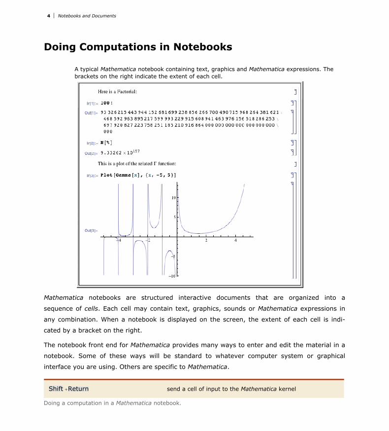
A typical Mathematica notebook containing text, graphics and Mathematica expressions. The brackets on the right indicate the extent of each cell.

Mathematica notebooks are structured interactive documents that are organized into a

sequence of cells. Each cell may contain text, graphics, sounds or Mathematica expressions in

any combination. When a notebook is displayed on the screen, the extent of each cell is indi-

cated by a bracket on the right.

The notebook front end for Mathematica provides many ways to enter and edit the material in a

notebook. Some of these ways will be standard to whatever computer system or graphical

interface you are using. Others are specific to Mathematica.

Shift +Return send a cell of input to the Mathematica kernel

Doing a computation in a Mathematica notebook.

Once you have prepared the material in a cell, you can send it as input to the Mathematica

kernel simply by pressing Shift+Return. The kernel will send back whatever output is gener-

ated, and the front end will create new cells in your notebook to display this output. Note that if

you have a numeric keypad on your keyboard, then you can use its Enter key as an alternative

to Shift+Return.


Once you have prepared the material in a cell, you can send it as input to the Mathematica

kernel simply by pressing Shift+Return. The kernel will send back whatever output is gener-

ated, and the front end will create new cells in your notebook to display this output. Note that if

you have a numeric keypad on your keyboard, then you can use its Enter key as an alternative

to Shift+Return.

Here is a cell ready to be sent as input to the Mathematica kernel.

The output from the computation is inserted in a new cell.

Most kinds of output that you get in Mathematica notebooks can readily be edited, just like

input. Usually Mathematica will convert the output cell into an input cell when you first start

editing it.

Once you have done the editing you want, you can typically just press Shift+Return to send

what you have created as input to the Mathematica kernel.

Here is a typical computation in a Mathematica notebook.

If you start editing the output cell, Mathematica will automatically change it to an input cell.

After you have edited the output, you can send it back as further input to the Mathematica kernel.


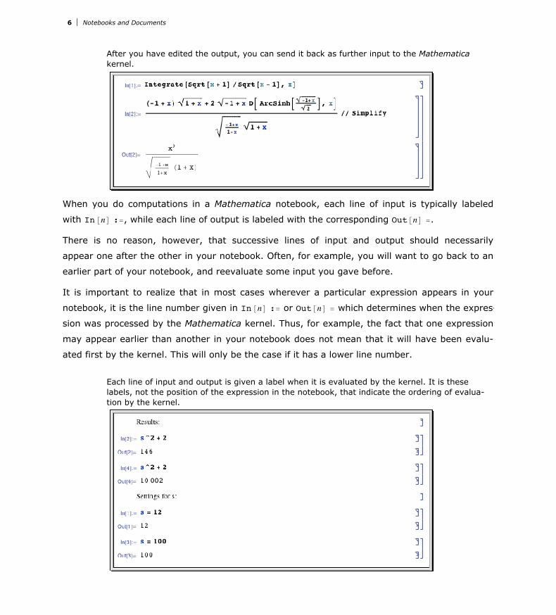
After you have edited the output, you can send it back as further input to the Mathematica kernel.

When you do computations in a Mathematica notebook, each line of input is typically labeled

with In@nD :=, while each line of output is labeled with the corresponding Out@nD =.

There is no reason, however, that successive lines of input and output should necessarily

appear one after the other in your notebook. Often, for example, you will want to go back to an

earlier part of your notebook, and reevaluate some input you gave before.

It is important to realize that in most cases wherever a particular expression appears in your

notebook, it is the line number given in In@nD := or Out@nD = which determines when the expres-

sion was processed by the Mathematica kernel. Thus, for example, the fact that one expression

may appear earlier than another in your notebook does not mean that it will have been evalu-

ated first by the kernel. This will only be the case if it has a lower line number.

Each line of input and output is given a label when it is evaluated by the kernel. It is these labels, not the position of the expression in the notebook, that indicate the ordering of evalua-tion by the kernel.

The exception to this rule is when an output contains the formatted results of a Dynamic or

Manipulate function. Such outputs will reevaluate in the kernel on an as-needed basis long

after the evaluation which initially created them. See "Dynamic Interactivity Language" for

more information on this functionality.


The exception to this rule is when an output contains the formatted results of a Dynamic or

Manipulate function. Such outputs will reevaluate in the kernel on an as-needed basis long

after the evaluation which initially created them. See "Dynamic Interactivity Language" for

more information on this functionality.

As you type, Mathematica applies syntax coloring to your input using its knowledge of the

structure of functions. The coloring highlights unmatched brackets and quotes, undefined global

symbols, local variables in functions and various programming errors. You can ask why Mathe-

matica colored your input by selecting it and using the Why the Coloring? item in the Help

menu.

If you make a mistake and try to enter input that the Mathematica kernel does not understand,

then the front end will produce a beep and emphasize any syntax errors in the input with color.

In general, you will get a beep whenever something goes wrong in the front end. You can find

out the origin of the beep using the Why the Beep? item in the Help menu.

Notebooks as Documents

Mathematica notebooks allow you to create documents that can be viewed interactively on

screen or printed on paper.

Particularly in larger notebooks, it is common to have chapters, sections and so on, each repre-

sented by groups of cells. The extent of these groups is indicated by a bracket on the right.


The grouping of cells in a notebook is indicated by nested brackets on the right.

A group of cells can be either open or closed. When it is open, you can see all the cells in it

explicitly. But when it is closed, you see only the cell around which the group is closed. Cell

groups are typically closed around the first or heading cell in the group, but you can close a

group around any cell in that group.

Large notebooks are often distributed with many closed groups of cells, so that when you first

look at the notebook, you see just an outline of its contents. You can then open parts you are

interested in by double-clicking the appropriate brackets.


Double-clicking the bracket that spans a group of cells closes the group, leaving only the first cell visible.

When a group is closed, the bracket for it has an arrow at the bottom. Double-clicking this arrow opens the group again.

Double-clicking the bracket of a cell that is not the first of a cell group closes the cell group around that cell and creates a bracket with up and down arrows (or only an up arrow if the cell was the last in the group).


Double-clicking the bracket of a cell that is not the first of a cell group closes the cell group around that cell and creates a bracket with up and down arrows (or only an up arrow if the cell was the last in the group).

Each cell within a notebook is assigned a particular style which indicates its role within the

notebook. Thus, for example, material intended as input to be executed by the Mathematica

kernel is typically in Input style, while text that is intended purely to be read is typically in

Text style.

The Mathematica front end provides menus and keyboard shortcuts for creating cells with

different styles, and for changing styles of existing cells.


This shows cells in various styles. The styles define not only the format of the cell contents, but also their placement and spacing.

By putting a cell in a particular style, you specify a whole collection of properties for the cell,

including for example how large and in what font text should be given.

The Mathematica front end allows you to modify such properties, either for complete cells, or

for specific material within cells.

Even within a cell of a particular style, the Mathematica front end allows a wide range of proper-ties to be modified separately.

Ordinary Mathematica notebooks can be read by non-Mathematica users using the free product,

Mathematica Player, which allows viewing and printing, but does not allow computations of any

kind to be performed. This product also supports notebook player files (.nbp), which have been

specially prepared by Wolfram Research to allow interaction with dynamic content such as the

output of Manipulate. For example, all the notebook content on The Wolfram Demonstrations

Project site is available as notebook player files.


Ordinary Mathematica notebooks can be read by non-Mathematica users using the free product,

Mathematica Player, which allows viewing and printing, but does not allow computations of any

kind to be performed. This product also supports notebook player files (.nbp), which have been

specially prepared by Wolfram Research to allow interaction with dynamic content such as the

output of Manipulate. For example, all the notebook content on The Wolfram Demonstrations

Project site is available as notebook player files.

Mathematica front end creating and editing Mathematica notebooks

Mathematica kernel doing computations in notebooks

Mathematica Player reading Mathematica notebooks and running Demonstrations

Programs required for different kinds of operations with notebooks.

Working with Cells

Mathematica notebooks consist of sequences of cells. The hierarchy of cells serves as a struc-

ture for organizing the information in a notebook, as well as specifying the overall look of the

notebook.

Font, color, spacing, and other properties of the appearance of cells are controlled using

stylesheets. The various kinds of cells associated with a notebook's stylesheet are listed in

Format Style. Mathematica comes with a collection of color and black-and-white stylesheets,

which are listed in the Format Stylesheet menu.

In a New Session:

When Mathematica is first started, it displays an empty notebook with a blinking cursor. You

can start typing right away.

The insertion point is indicated by the cell insertion bar, a solid gray line with a small black

cursor running horizontally across the notebook. The cell insertion bar is the place where new

cells will be created, either as you type or programmatically. To set the position of the insertion

bar, click in the notebook.


The insertion point is indicated by the cell insertion bar, a solid gray line with a small black

cursor running horizontally across the notebook. The cell insertion bar is the place where new

cells will be created, either as you type or programmatically. To set the position of the insertion

bar, click in the notebook.

To Create a New Cell:

Move the pointer in the notebook window until it becomes a horizontal I-beam.

Click, and a cell insertion bar will appear; start typing. By default, new cells are Mathematica

input cells.


To Create a New Cell to Hold Ordinary Text:

Click in the notebook to get a cell insertion bar. Choose Format Style Text or use the

keyboard shortcut Cmd+7.

When you start typing, a text cell bracket appears.

To Change the Style of a Cell:

Click the cell bracket. The bracket is highlighted.

Select a style from Format Style. The cell will immediately reflect the change.


Alternatively, you can simultaneously press Cmd with one of the numbered keys, 0 through 9,

to select a style.

Choose Window Show Toolbar to get a toolbar at the top of the notebook.

Choose Window Show Ruler to get a ruler at the top of the notebook.


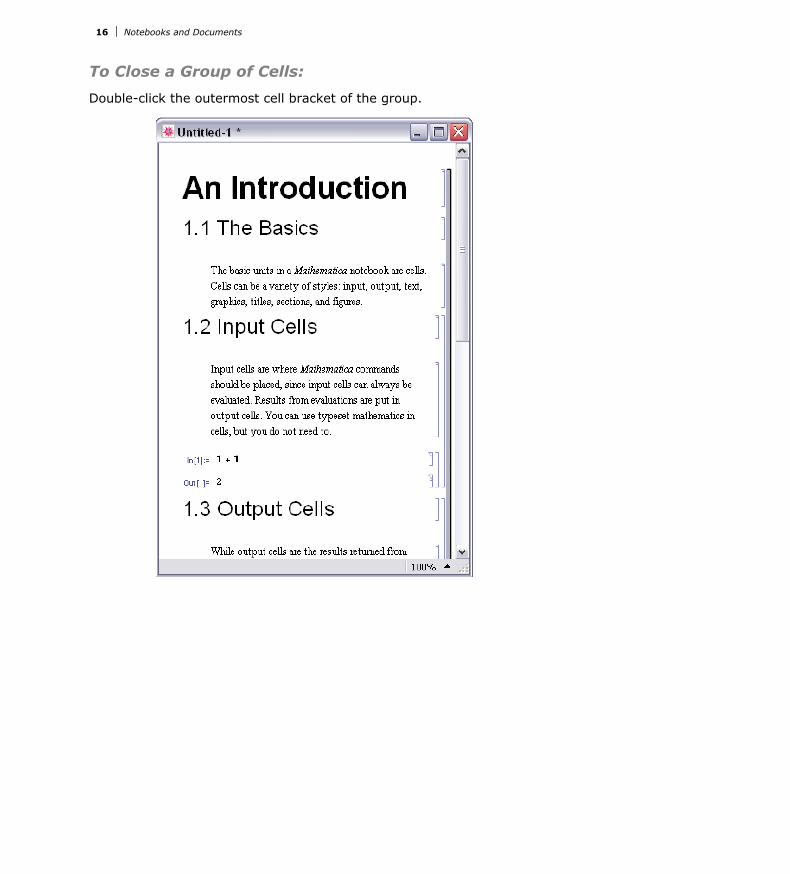
To Close a Group of Cells:

Double-click the outermost cell bracket of the group.


When a group is closed, only the first cell in the group is displayed by default. The group

bracket is shown with a triangular flag at the bottom.


To specify which cells remain visible when the cell group is closed, select those cells and double-

click to close the group. The closed group bracket is shown with triangular flags at the top and

bottom if the visible cells are within a cell group, or with a triangular flag at the top if they are

at the end of a cell group.


To Open a Group of Cells:

Double-click a closed group’s cell bracket.

To Print a Notebook:

Choose File Print. The notebook style will be automatically optimized for printing.

To Change the Overall Look of a Notebook:


Choose Format Stylesheet. Select a stylesheet from the menu. All cells in the notebook will

change appearance, based on the definitions in the new stylesheet.

Use Format Edit Stylesheet to customize stylesheets for Mathematica notebooks.

Changes to a notebook that only involve opening or closing cell groups will not cause the front

end to ask you if you want to save such changes when you close the notebook before saving.

To save these changes, use File Save before you close the notebook or quit Mathematica.

To close a notebook, click the Close button in the title bar. You will be prompted to save any

unsaved changes.

On Windows, to close notebooks without being prompted to save, hold down the Shift key when

clicking the Close box.

The Option Inspector


The Option Inspector

Introduction

Many aspects of the Mathematica front end, such as the styles of cells, the appearance of

notebooks, or the parameters used in typesetting, are controlled by options. For example, text

attributes such as size, font, and color each correspond to a separate option. You can set

options by directly editing the expression for a cell or notebook. But in most cases it is simpler

to use the Option Inspector.

The Option Inspector is a special tool for viewing and modifying option settings. It provides a

comprehensive listing of all front end options, grouped according to their function. You can

specify not only the setting for an option, but also the level at which it will take effect: globally,

for an entire notebook, or for a selection.

To use the Option Inspector, choose Format Option Inspector. This brings up a dialog box

with two popup menus on top. The popup menu on the left specifies the level at which options

will take effect. The popup menu on the right allows you to choose if you want the options listed

by category, alphabetically, or as text.

Inheritance of Options

The Option Inspector allows you to set the value of an option on three different levels. In increas-

ing order of precedence, the levels are as follows.

Global Preferences - settings for the entire application

Selected Notebook - settings for an entire notebook

Selection - settings for the current selection, e.g. for a group of cells, a single cell, or text

within a cell


The levels lower in the hierarchy inherit their options from the level immediately above them.

For example, if a notebook has the option Editable set to True, by default all cells in the

notebook will be editable.

You can, however, override the inherited value of an option by explicitly changing its value. For

example, if you do not want a particular cell in your notebook to be editable, you can select the

cell and set Editable to False. This inheritance property of options provides you with a great

deal of control over the behavior of the front end, since you can set any option to have different

values at each level, as required.

Note: At each level, only the options that can be set at that level are listed in the Option Inspec-

tor. All other options appear dimmed, indicating that they cannot be changed unless you go to

a higher or lower level.

Searching for an Option

To search for a specific option, begin typing its name in the text field. The Option Inspector

goes to the first matching option. Press Enter to go to the next matching item on the list. (On

Macintosh, the Option Inspector displays all matching options at once).

Each line in the list of options gives the option name followed by its current value. You can

change the option's value by choosing from the popup menu next to the option setting, or by

selecting the option and clicking the value, typing over it, and pressing Enter.

When you start Mathematica for the first time, the values of all the options are set to their

default values. Each time you modify one of the options, a symbol appears next to it, indicating

that the value has been changed. Clicking the symbol resets the option to its default value.


Setting Options: An Example

Suppose you want to draw a frame around a cell. The option that controls this property of a cell

is called CellFrame.

To Draw a Frame around a Cell:

1. Select the cell by clicking the cell bracket.

2. Choose Format Option Inspector to open the Option Inspector window.

3. Choose Selection from the first popup menu.

4. Click Cell Options Display Options. This gives a list of all options that control how acell is displayed in the notebook.

5. Type True into the value field next to the option CellFrame. An icon appears next to theoption, indicating that its value has been changed. The cell that you selected now has aframe drawn around it.

Alternatively, you can begin typing "cellframe" in the text field. This leads you directly to the

CellFrame option without having to search by category. This feature provides a useful way to

locate an option if you are unsure of the category it belongs in.

Notebook History Dialog

This dialog displays information regarding the editing times of the input notebook. This is a

"live" dialog that dynamically updates as changes are made to the notebook. It can be accessed

through Cell Notebook History.


The time information is saved in each cell of the notebook, in the form of a list of numbers

and/or pairs of numbers.

Cell[BoxData["123"], "Input", CellChangeTimes->3363263352.09502, 3363263354.03695, 3363263406.22268, 3363263441.939 ]

Each number represents the exact time of an edit, in absolute time units. A list of pairs indi-

cates multiple edits that have occurred during this interval.

Consecutive edits are recorded as an interval if they happen within a set time period. This

period is determined by CellChangeTimesMergeInterval, which can be set through the Option

Inspector or the Advanced section of the Preferences dialog. The default is 30 seconds.

The notebook history tracking feature can be turned off at the global level by using the Prefer-

ences dialog or by setting TrackCellChangeTimes to False.


Features

Controls

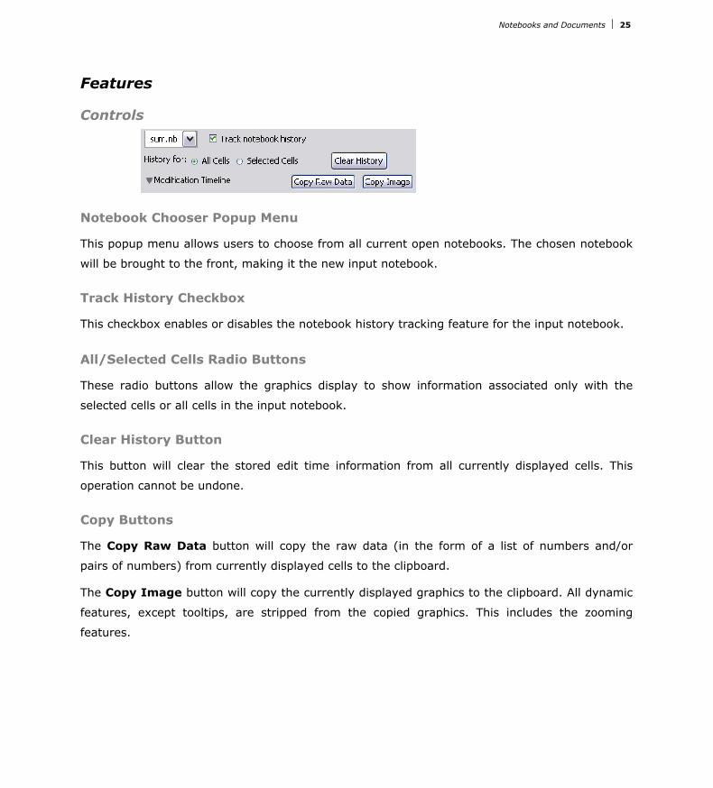
Notebook Chooser Popup Menu

This popup menu allows users to choose from all current open notebooks. The chosen notebook

will be brought to the front, making it the new input notebook.

Track History Checkbox

This checkbox enables or disables the notebook history tracking feature for the input notebook.

All/Selected Cells Radio Buttons

These radio buttons allow the graphics display to show information associated only with the

selected cells or all cells in the input notebook.

Clear History Button

This button will clear the stored edit time information from all currently displayed cells. This

operation cannot be undone.

Copy Buttons

The Copy Raw Data button will copy the raw data (in the form of a list of numbers and/or

pairs of numbers) from currently displayed cells to the clipboard.

The Copy Image button will copy the currently displayed graphics to the clipboard. All dynamic

features, except tooltips, are stripped from the copied graphics. This includes the zooming

features.


Graphics

The graphics display plots cells versus time. Each cell in the notebook corresponds to each row

on the y axis. The corresponding edit times are plotted as points, while edit intervals are repre-

sented by lines.

Mouse Events

As you mouse over the graphics, the mouse tooltip may provide some useful details for the

following elements:

† Each row on the y axis will display the corresponding cell's contents.

† Points will display the exact time of the edit (which corresponds to the computer clock atthe time of edit).

† Lines will display the length of the edit interval (this value may be greater than theCellChangeTimesMergeInterval value).

Clicking a highlighted row will select the corresponding cell in the input notebook if and only if

the selection-only checkbox is unchecked.


Zooming

The graphics display comes with a couple of zooming features for the time axis:

† The blue triangles at the bottom can be dragged to change the plotted time interval. Usethe middle diamond to pan the graphics using the same time interval.

† Clicking any time label blocks will zoom into that interval of time. With this feature, userscan actually zoom down to the last second (which may be out of range with the previouszoom feature).

† Clicking the shaded area will undo the last zoom action. Click outside the shaded area torevert to showing the entire time interval.

Summary

The summary is a concise, overall display of relevant cell information. This display also respects

the setting of the selection-only checkbox.


Input and Output in Notebooks

Entering Greek Letters

click on a use a button in a palette

\[Alpha] use a full name

Esc aEsc or Esc alphaEsc use a standard alias (shown below as EscaEsc)

Esc \alpha Esc use a TEX alias

Esc & alpha;Esc use an HTML alias

Ways to enter Greek letters in a notebook.

Here is a palette for entering common Greek letters.

You can use Greek letters just like the ordinary letters that you type on your keyboard.

In[1]:= Expand@Ha + bL^3D

Out[1]= a3 + 3 a2 b + 3 a b2 + b3


There are several ways to enter Greek letters. This input uses full names.

In[2]:= Expand@Ha + bL^3D

Out[2]= a3 + 3 a2 b + 3 a b2 + b3

Esc ThetaEsc

Esc

Esc

Esc

Esc PhiEsc

Esc ChiEsc

Esc PsiEsc

Esc OmegaEsc

Commonly used Greek letters. TeX aliases are not listed explicitly.


full name aliases

Α \[Alpha] Esc aEsc, Esc alphaEsc

Β \[Beta] Esc bEsc, Esc betaEsc

Γ \[Gamma] Esc gEsc, Esc gammaEsc

∆ \[Delta] Esc dEsc, Esc deltaEsc

Ε \[Epsilon] Esc eEsc, Esc epsilonEsc

Ζ \[Zeta] Esc zEsc, Esc zetaEsc

Η \[Eta] Esc hEsc, Esc etEsc, Esc etaEsc

Θ \[Theta] Esc qEsc, Esc thEsc, Esc thetaEsc

Κ \[Kappa] Esc kEsc, Esc kappaEsc

Λ \[Lambda] Esc lEsc, Esc lambdaEsc

Μ \[Mu] Esc mEsc, Esc muEsc

Ν \[Nu] Esc nEsc, Esc nuEsc

Ξ \[Xi] Esc xEsc, Esc xiEsc

Π \[Pi] Esc pEsc, Esc piEsc

Ρ \[Rho] Esc rEsc, Esc rhoEsc

Σ \[Sigma] Esc sEsc, Esc sigmaEsc

Τ \[Tau] Esc tEsc, Esc tauEsc

Φ \[Phi] Esc fEsc, Esc phEsc, Esc phiEsc

j \[CurlyPhi] Esc jEsc, Esc cphEsc, Esc cphiEsc

Χ \[Chi] Esc cEsc, Esc chEsc, Esc chiEsc

Ψ \[Psi] Esc yEsc, Esc psEsc, Esc psiEsc

Ω \[Omega] Esc oEsc, Esc wEsc, Esc omegaEsc

full name aliases

G \[CapitalGamma] Esc GEsc, Esc GammaEsc

D \[CapitalDelta] Esc DEsc, Esc DeltaEsc

Q \[CapitalTheta] Esc QEsc, Esc ThEsc, Esc ThetaEsc

L \[CapitalLambda] Esc LEsc, Esc LambdaEsc

P \[CapitalPi] Esc PEsc, Esc PiEsc

S \[CapitalSigma] Esc SEsc, Esc SigmaEsc

U \[CapitalUpsilon] Esc UEsc, Esc UpsilonEsc

F \[CapitalPhi] Esc FEsc, Esc PhEsc, Esc PhiEsc

C \[CapitalChi] Esc CEsc, Esc ChEsc, Esc ChiEsc

Y \[CapitalPsi] Esc YEsc, Esc PsEsc, Esc PsiEsc

W \[CapitalOmega] Esc OEsc, Esc WEsc, Esc OmegaEsc

Note that in Mathematica the letter p stands for Pi. None of the other Greek letters have spe-

cial meanings.

p stands for Pi.

In[3]:= N@pD

Out[3]= 3.14159

You can use Greek letters either on their own or with other letters.

In[4]:= Expand@HRab + XL^4D

Out[4]= Rab4 + 4 Rab3 X + 6 Rab2 X2 + 4 Rab X3 + X4

The symbol pa is not related to the symbol p.

In[5]:= Factor@pa^4 - 1D

Out[5]= H-1 + paL H1 + paL I1 + pa2M

Entering Two-Dimensional Input

When Mathematica reads the text x^y, it interprets it as x raised to the power y.

In[1]:= x^y

Out[1]= xy

In a notebook, you can also give the two-dimensional input xy directly. Mathematica again interprets this as a power.

In[2]:= xy

Out[2]= xy

One way to enter a two-dimensional form such as xy into a Mathematica notebook is to paste

this form into the notebook by clicking the appropriate button in the palette.


Here is a palette for entering some common two-dimensional notations.

There are also several ways to enter two-dimensional forms directly from the keyboard.

x Ctrl+^ y Ctrl+Space use control keys that exist on most keyboards

x Ctrl+6 y Ctrl+Space use control keys that should exist on all keyboards

Ways to enter a superscript directly from the keyboard.

You type Ctrl+^ by holding down the Control key, then pressing the ^ key. As soon as you do

this, your cursor will jump to a superscript position. You can then type anything you want and it

will appear in that position.


When you have finished, press Ctrl+Space to move back down from the superscript position.

You type Ctrl+Space by holding down the Control key, then pressing the Space bar.

This sequence of keystrokes enters xy.

In[3]:= x Ctrl+^ y

Out[3]= xy

Here the whole expression y + z is in the superscript.

In[4]:= x Ctrl+^ y + z

Out[4]= xy+z

Pressing Ctrl+Space takes you down from the superscript.

In[5]:= x Ctrl+^ y Ctrl+Space + z

Out[5]= xy + z

You can remember the fact that Ctrl+^ gives you a superscript by thinking of Ctrl+^ as just a

more immediate form of ^. When you type x^y, Mathematica will leave this one-dimensional

form unchanged until you explicitly process it. But if you type x Ctrl+^ y then Mathematica will

immediately give you a superscript.

On a standard English-language keyboard, the character ^ appears as the shifted version of 6.

Mathematica therefore accepts Ctrl+6 as an alternative to Ctrl+^. Note that if you are using

something other than a standard English-language keyboard, Mathematica will almost always

accept Ctrl+6 but may not accept Ctrl+^.

x Ctrl+_ y Ctrl+Space use control keys that exist on most keyboards

x Ctrl+- y Ctrl+Space use control keys that should exist on all keyboards

Ways to enter a subscript directly from the keyboard.


Subscripts in Mathematica work very much like superscripts. However, whereas Mathematica

automatically interprets xy as x raised to the power y, it has no similar interpretation for xy.

Instead, it just treats xy as a purely symbolic object.

This enters y as a subscript.

In[6]:= x Ctrl+_ yOut[6]= xy

Here is the usual one-dimensional Mathematica input that gives the same output expression.

In[7]:= Subscript@x, yD

Out[7]= xy

x Ctrl+/ y Ctrl+Space use control keys

How to enter a built-up fraction directly from the keyboard.

This enters the built-up fraction xy.

In[8]:= x Ctrl+/ y

Out[8]= x

y

Here the whole y + z goes into the denominator.

In[9]:= x Ctrl+/ y + z

Out[9]= x

y + z

But pressing Ctrl+Space takes you out of the denominator, so the +z does not appear in the denominator.

In[10]:= x Ctrl+/ y Ctrl+Space + z

Out[10]= x

y+ z


Mathematica automatically interprets a built-up fraction as a division.

In[11]:=8888

2222Out[11]= 4

Ctrl+@ x Ctrl+Space use control keys that exist on most keyboards

Ctrl+2 x Ctrl+Space use control keys that should exist on all keyboards

Ways to enter a square root directly from the keyboard.

This enters a square root.

In[12]:= Ctrl+@ x + y

Out[12]= x + y

Ctrl+Space takes you out of the square root.

In[13]:= Ctrl+@ x Ctrl+Space + y

Out[13]= x + y

Here is the usual one-dimensional Mathematica input that gives the same output expression.

In[14]:= Sqrt@xD + y

Out[14]= x + y

Ctrl+^ or Ctrl+6 go to the superscript position

Ctrl+_ or Ctrl+- go to the subscript position

Ctrl+@ or Ctrl+2 go into a square root

Ctrl+% or Ctrl+5 go from subscript to superscript or vice versa, or to the exponent position in a root

Ctrl+/ go to the denominator for a fraction

Ctrl+Space return from a special position

Special input forms based on control characters. The second forms given should work on any keyboard.


This puts both a subscript and a superscript on x.

In[15]:= x Ctrl+^ y Ctrl+% z

Out[15]= xzy

Here is another way to enter the same expression.

In[16]:= x Ctrl+_ z Ctrl+% y

Out[16]= xzy

The same procedure can be used to enter a definite integral.

In[17]:= Esc intEsc Ctrl+_ 0 Ctrl+% 1 Ctrl+Space f[x] Esc ddEsc x

Out[17]= ‡0

1f@xD „x

In addition to subscripts and superscripts, Mathematica also supports the notion of underscripts

and overscripts~elements that go directly underneath or above. Among other things, you can

use underscripts and overscripts to enter the limits of sums and products.

x Ctrl+Plus y Ctrl+Space or x Ctrl+= y Ctrl+Space

create an underscript xy

x Ctrl+& y Ctrl+Space or x Ctrl+7 y Ctrl+Space

create an overscript xy

Creating underscripts and overscripts.

Here is a way to enter a summation.

In[18]:= Esc sumEsc Ctrl+Plus x=0 Ctrl+% n Ctrl+Space f[x]

Out[18]= ‚

x=0

n

f@xD


Editing and Evaluating Two-Dimensional Expressions

When you see a two-dimensional expression on the screen, you can edit it much as you would

edit text. You can for example place your cursor somewhere and start typing. Or you can select

a part of the expression, then remove it using the Delete key, or insert a new version by typing

it in.

In addition to ordinary text editing features, there are some keys that you can use to move

around in two-dimensional expressions.

Ctrl+. select the next larger subexpression

Ctrl+Space move to the right of the current structure

Ø move to the next character

move to the previous character

Ways to move around in two-dimensional expressions.

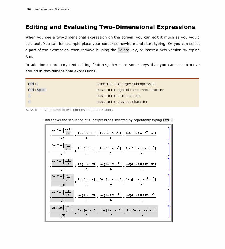
This shows the sequence of subexpressions selected by repeatedly typing Ctrl+..


Shift+Return evaluate the whole current cell

Shift+Ctrl+Enter (Windows/Unix/Linux) or Cmd+Return (Mac OS X)

evaluate only the selected subexpression

Ways to evaluate two-dimensional expressions.

In most computations, you will want to go from one step to the next by taking the whole expres-

sion that you have generated, and then evaluating it. But if for example you are trying to manip-

ulate a single formula to put it into a particular form, you may instead find it more convenient

to perform a sequence of operations separately on different parts of the expression.

You do this by selecting each part you want to operate on, then inserting the operation you

want to perform, then using Shift+Ctrl+Enter for Windows/Unix/Linux or Cmd+Return for Mac

OS X.

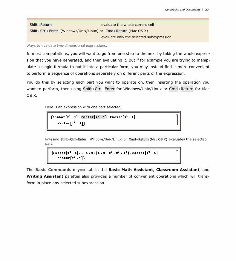
Here is an expression with one part selected.

Pressing Shift+Ctrl+Enter (Windows/Unix/Linux) or Cmd+Return (Mac OS X) evaluates the selected part.

The Basic Commands y=x tab in the Basic Math Assistant, Classroom Assistant, and

Writing Assistant palettes also provides a number of convenient operations which will trans-

form in place any selected subexpression.


Entering Formulas

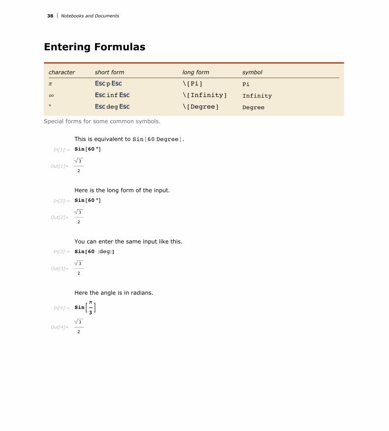
character short form long form symbol

p Esc pEsc \[Pi] Pi

¶ Esc infEsc \[Infinity] Infinity

° Esc degEsc \[Degree] Degree

Special forms for some common symbols.

This is equivalent to Sin@60 DegreeD.

In[1]:= Sin@60 °D

Out[1]= 3

2

Here is the long form of the input.

In[2]:= Sin@60 °D

Out[2]= 3

2

You can enter the same input like this.

In[3]:= Sin[60 ÇdegÇ]

Out[3]= 3

2

Here the angle is in radians.

In[4]:= SinBp

3F

Out[4]= 3

2


special characters short form long form ordinary characters

x§y x Esc <=Esc y x \@LessEqualD y x <= y

x¥y x Esc >=Esc y x\@GreaterEqualDy

x >= y

x≠y x Esc !=Esc y x \@NotEqualD y x != y

xœy x Esc elEsc y x \@ElementD y Element@x,yD

xØy x Esc ->Esc y x \@RuleD y x -> y

Special forms for a few operators. "Operator Input Forms" gives a complete list.

Here the replacement rule is entered using two ordinary characters, as ->.

In[5]:= x ê Hx + 1L ê. x -> 3 + y

Out[5]= 3 + y

4 + y

This means exactly the same.

In[6]:= x ê Hx + 1L ê. x Ø 3 + y

Out[6]= 3 + y

4 + y

As does this.

In[7]:= x/(x+1) /. x Esc ->Esc 3 + y

Out[7]= 3 + y

4 + y

When you type the ordinary-character form for certain operators, the front end automatically

replaces them with the special-character form. For instance, when you type the last three

examples, the front end automatically substitutes the Ø character for ->.

The special arrow form Ø is by default also used for output.

In[8]:= Solve@x^2 == 1, xD

Out[8]= 88x Ø -1<, 8x Ø 1<<


special characters short form long form ordinary characters

x ¸ y x Esc divEsc y x \@DivideD y x ê y

x µ y x Esc *Esc y x \@TimesD y x * y

x ä y x EsccrossEsc y

x \@CrossD y Cross@x,yD

x ã y x Esc ==Esc y x \@EqualD y x == y

x y x Esc l =Esc y x \@LongEqualD y x == y

x Ï y x Esc &&Esc y x \@AndD y x && y

x Í y x Esc »»Esc y x \@OrD y x »» y

Ÿ x Esc !Esc x \@NotD x ! x

x fl y x Esc =>Esc y x \@ImpliesD y x => y

x ‹ y x Esc unEsc y x \@UnionD y Union@x,yD

x › y x EscinterEsc y

x \@IntersectionD y Intersection@x,yD

xy x Esc ,Esc y x \@InvisibleCommaD y x , y

f x f Esc üEsc x f\@InvisibleApplicatiÖ

onDx

f ü x or f@xD

x yz

x Esc +Esc yz

x \@ImplicitPlusD yz

x + y ê z

Some operators with special forms used for input but not output.

Mathematica understands ¸, but does not use it by default for output.

In[9]:= x ¸ y

Out[9]= x

y

Many of the forms of input discussed here use special characters, but otherwise just consist of

ordinary one-dimensional lines of text. Mathematica notebooks, however, also make it possible

to use two-dimensional forms of input.


two-dimensional one-dimensional

xy x^y powerxy

xêy division

x Sqrt@xD square root

xn

x^H1ênL nth root

⁄i=iminimax f Sum@ f,8i,imin,imax<D sum

¤i=iminimax f Product@ f,8i,imin,imax<D product

Ÿ f „ x Integrate@ f,xD indefinite integral

Ÿxminxmax f „ x Integrate@ f,8x,xmin,xmax<D definite integral

∂x f D@ f,xD partial derivative

∂x,y f D@ f,x,yD multivariate partial derivative

z Conjugate@xD complex conjugate

m Transpose@mD transpose

mæ ConjugateTranspose@mD conjugate transpose

expr@@ i, j,… DD Part@expr,i, j,…D part extraction

Some two-dimensional forms that can be used in Mathematica notebooks.

You can enter two-dimensional forms using any of the mechanisms discussed in "Entering Two-

Dimensional Input". Note that upper and lower limits for sums and products must be entered as

overscripts and underscripts~not superscripts and subscripts.

This enters an indefinite integral. Note the use of Esc ddEsc to enter the “differential d”.

In[10]:= Esc intEsc f[x] Esc ddEsc x

Out[10]= ‡ f@xD „x

Here is an indefinite integral that can be explicitly evaluated.

In[11]:= ‡ ExpA-x2E „x

Out[11]= 1

2p Erf@xD


Here is the usual Mathematica input for this integral.

In[12]:= Integrate@Exp@-x^2D, xD

Out[12]= 1

2p Erf@xD

short form long form

Esc sum Esc \@SumD summation sign ⁄

Esc prodEsc \@ProductD product sign ¤

Esc intEsc \@IntegralD integral sign Ÿ

Esc ddEsc \@DifferentialDD special „ for use in integrals

Esc pdEsc \@PartialDD partial derivative operator ∂

Esc coEsc \@ConjugateD conjugate symbol Esc trEsc \@TransposeD transpose symbol Esc ctEsc \@ConjugateTransposeD conjugate transpose symbol æEsc @@Esc \@LeftDoubleBracketD part brackets

Some special characters used in entering formulas. "Mathematical and Other Notation" gives a complete list.

You should realize that even though a summation sign can look almost identical to a capital

sigma it is treated in a very different way by Mathematica. The point is that a sigma is just a

letter; but a summation sign is an operator which tells Mathematica to perform a Sum operation.

Capital sigma is just a letter.

In[13]:= a + S^2

Out[13]= a + S2

A summation sign, on the other hand, is an operator.

In[14]:= Esc sumEsc Ctrl++ n=0 Ctrl+% m Ctrl+Space 1/f[n]

Out[14]= ‚

n=0

m 1

f@nD

Much as Mathematica distinguishes between a summation sign and a capital sigma, it also

distinguishes between an ordinary d, the “partial d” ∂ that is used for taking derivatives, and

the special “differential d” „ that is used in the standard notation for integrals. It is crucial that

you use the differential „~entered as Esc ddEsc~when you type in an integral. If you try to use

an ordinary d, Mathematica will just interpret this as a symbol called d~it will not understand

that you are entering the second part of an integration operator.


Much as Mathematica distinguishes between a summation sign and a capital sigma, it also

distinguishes between an ordinary d, the “partial d” ∂ that is used for taking derivatives, and

the special “differential d” „ that is used in the standard notation for integrals. It is crucial that

you use the differential „~entered as Esc ddEsc~when you type in an integral. If you try to use

an ordinary d, Mathematica will just interpret this as a symbol called d~it will not understand

that you are entering the second part of an integration operator.

This computes the derivative of xn.

In[15]:= ∂xxn

Out[15]= n x-1+n

Here is the same derivative specified in ordinary one-dimensional form.

In[16]:= D@x^n, xD

Out[16]= n x-1+n

This computes the third derivative.

In[17]:= ∂x,x,xxn

Out[17]= H-2 + nL H-1 + nL n x-3+n

Here is the equivalent one-dimensional input form.

In[18]:= D@x^n, x, x, xD

Out[18]= H-2 + nL H-1 + nL n x-3+n

Entering Tables and Matrices

The Mathematica front end provides an Insert Table/Matrix submenu for creating and

editing arrays with any specified number of rows and columns. Once you have such an array,

you can edit it to fill in whatever elements you want.

Mathematica treats an array like this as a matrix represented by a list of lists.

In[1]:=a b c1 2 3

Out[1]= 88a, b, c<, 81, 2, 3<<

Putting parentheses around the array makes it look more like a matrix, but does not affect its interpretation.

In[2]:= Ka b c1 2 3

O

Out[2]= 88a, b, c<, 81, 2, 3<<

Using MatrixForm tells Mathematica to display the result of the Transpose as a matrix.


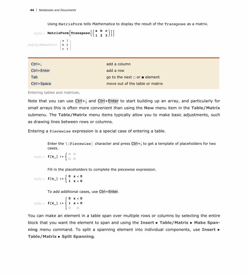
Using MatrixForm tells Mathematica to display the result of the Transpose as a matrix.

In[3]:= MatrixFormBTransposeBKa b c1 2 3

OFF

Out[3]//MatrixForm=a 1b 2c 3

Ctrl+, add a column

Ctrl+Enter add a row

Tab go to the next Ñ or É element

Ctrl+Space move out of the table or matrix

Entering tables and matrices.

Note that you can use Ctrl+, and Ctrl+Enter to start building up an array, and particularly for

small arrays this is often more convenient than using the New menu item in the Table/Matrix

submenu. The Table/Matrix menu items typically allow you to make basic adjustments, such

as drawing lines between rows or columns.

Entering a Piecewise expression is a special case of entering a table.

Enter the \@PiecewiseD character and press Ctrl+, to get a template of placeholders for two cases.

In[4]:= f@x_D := Ñ ÑÑ Ñ

Fill in the placeholders to complete the piecewise expression.

In[5]:= f@x_D := 0 x < 01 x = 0

To add additional cases, use Ctrl+Enter.

In[6]:= f@x_D :=0 x < 01 x = 0Ñ Ñ

You can make an element in a table span over multiple rows or columns by selecting the entire

block that you want the element to span and using the Insert Table/Matrix Make Span-

ning menu command. To split a spanning element into individual components, use Insert Table/Matrix Split Spanning.


To make the top element span across both columns, first select the row.

In[7]:=x Ñy z

Now use the Make Spanning menu command.

In[8]:=x

y z

Subscripts, Bars and Other Modifiers

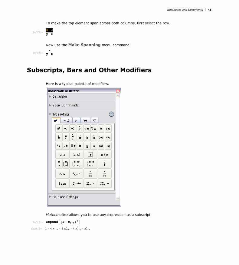
Here is a typical palette of modifiers.

Mathematica allows you to use any expression as a subscript.

In[1]:= ExpandAH1 + x1+nL4E

Out[1]= 1 + 4 x1+n + 6 x1+n2 + 4 x1+n

3 + x1+n4


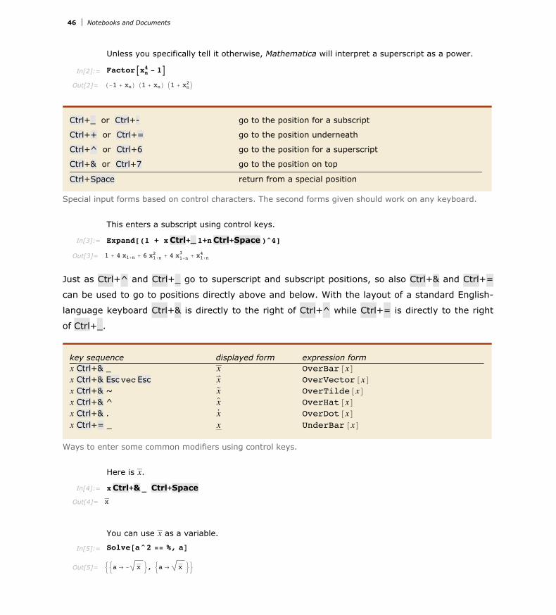
Unless you specifically tell it otherwise, Mathematica will interpret a superscript as a power.

In[2]:= FactorAxn4 - 1E

Out[2]= H-1 + xnL H1 + xnL I1 + xn2M

Ctrl+_ or Ctrl+- go to the position for a subscript

Ctrl++ or Ctrl+= go to the position underneath

Ctrl+^ or Ctrl+6 go to the position for a superscript

Ctrl+& or Ctrl+7 go to the position on top

Ctrl+Space return from a special position

Special input forms based on control characters. The second forms given should work on any keyboard.

This enters a subscript using control keys.

In[3]:= Expand[(1 + xCtrl+_1+nCtrl+Space )^4]

Out[3]= 1 + 4 x1+n + 6 x1+n2 + 4 x1+n

3 + x1+n4

Just as Ctrl+^ and Ctrl+_ go to superscript and subscript positions, so also Ctrl+& and Ctrl+=

can be used to go to positions directly above and below. With the layout of a standard English-

language keyboard Ctrl+& is directly to the right of Ctrl+^ while Ctrl+= is directly to the right

of Ctrl+_.

key sequence displayed form expression formx Ctrl+& _ x OverBar@xDx Ctrl+& Esc vecEsc x” OverVector@xDx Ctrl+& ~ xè OverTilde@xDx Ctrl+& ^ x` OverHat@xDx Ctrl+& . x° OverDot@xDx Ctrl+= _ x UnderBar@xD

Ways to enter some common modifiers using control keys.

Here is x.

In[4]:= xCtrl+&_ Ctrl+Space

Out[4]= x

You can use x as a variable.

In[5]:= Solve@a^2 == %, aD

Out[5]= ::a Ø - x >, :a Ø x >>

Non-English Characters and Keyboards


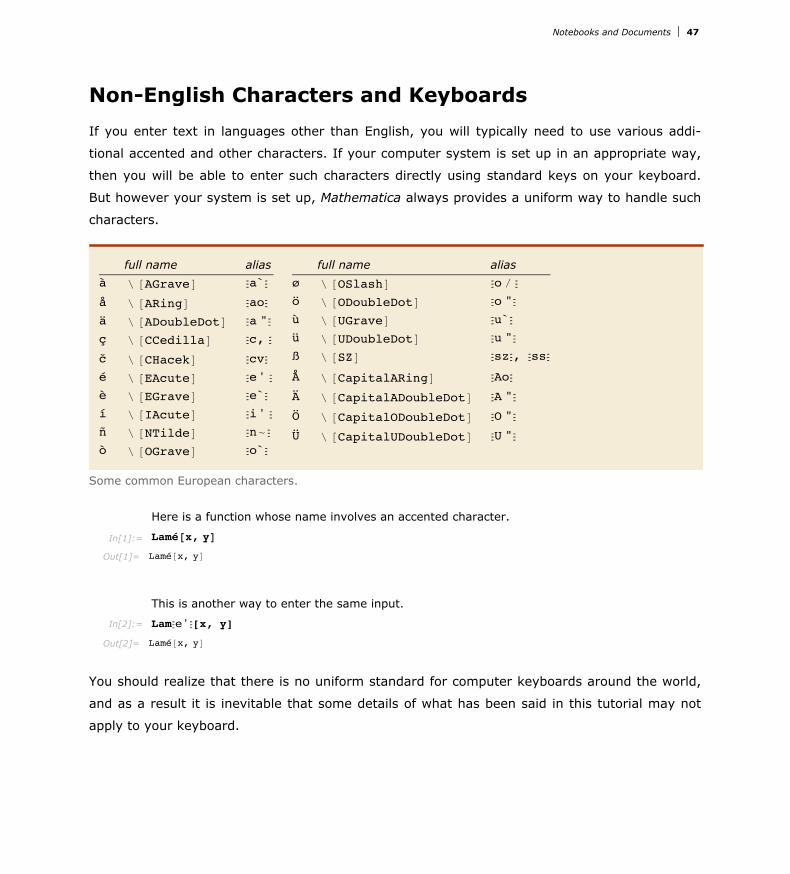
Non-English Characters and Keyboards

If you enter text in languages other than English, you will typically need to use various addi-

tional accented and other characters. If your computer system is set up in an appropriate way,

then you will be able to enter such characters directly using standard keys on your keyboard.

But however your system is set up, Mathematica always provides a uniform way to handle such

characters.

full name aliasà î @AGraveD Ça`Ç

å î @ARingD ÇaoÇ

ä î @ADoubleDotD Ça "Çç î @CCedillaD Çc, Ç

č î @CHacekD ÇcvÇé î @EAcuteD Çe' Ç

è î @EGraveD Çe`Çí î @IAcuteD Çi' Ç

ñ î @NTildeD Çn~Çò î @OGraveD Ço`Ç

full name aliasø î @OSlashD Ço ê Ç

ö î @ODoubleDotD Ço "Çù î @UGraveD Çu`Çü î @UDoubleDotD Çu "Çß î @SZD ÇszÇ, ÇssÇ

Å î @CapitalARingD ÇAoÇ

Ä î @CapitalADoubleDotD ÇA "Ç

Ö î @CapitalODoubleDotD ÇO "Ç

Ü î @CapitalUDoubleDotD ÇU "Ç

Some common European characters.

Here is a function whose name involves an accented character.

In[1]:= Lamé@x, yD

Out[1]= Lamé@x, yD

This is another way to enter the same input.

In[2]:= LamÇe'Ç[x, y]

Out[2]= Lamé@x, yD

You should realize that there is no uniform standard for computer keyboards around the world,

and as a result it is inevitable that some details of what has been said in this tutorial may not

apply to your keyboard.


In particular, the identification for example of Ctrl+6 with Ctrl+^ is valid only for keyboards on

which ^ appears as Shift+6. On other keyboards, Mathematica uses Ctrl+6 to go to a super-

script position, but not necessarily Ctrl+^.

Regardless of how your keyboard is set up you can always use palettes or menu items to set up

superscripts and other kinds of notation. And assuming you have some way to enter characters

such as î, you can always give input using full names such as \[Infinity].

Other Mathematical Notation

Mathematica supports an extremely wide range of mathematical notation, although often it

does not assign a pre-defined meaning to it. Thus, for example, you can enter an expression

such as x ⊕ y, but Mathematica will not initially make any assumption about what you mean by

⊕.

Mathematica knows that ⊕ is an operator, but it does not initially assign any specific meaning to it.

In[1]:= 817 ⊕ 5, 8 ⊕ 3<

Out[1]= 817⊕5, 8⊕3<

This gives Mathematica a definition for what the ⊕ operator does.

In[2]:= x_ ⊕ y_ := Mod@x + y, 2D

Now Mathematica can evaluate ⊕ operations.

In[3]:= 817 ⊕ 5, 8 ⊕ 3<

Out[3]= 80, 1<


full name alias⊕ \@CirclePlusD Çc+Ç

⊗ \@CircleTimesD Çc*Ç

± \@PlusMinusD Ç+-Ç

Ô \@WedgeD Ç^Ç

Ó \@VeeD ÇvÇ

> \@TildeEqualD Ç~=Ç

º \@TildeTildeD Ç~~Ç

~ \@TildeD Ç~Ç

∝ \@ProportionalD ÇpropÇ

ª \@CongruentD Ç===Ç

t \@GreaterTildeD Ç>~Ç

p \@GreaterGreaterDê \@SucceedsD@ \@RightTriangleD

full name aliasö \@LongRightArrowD Ç-->Ç

\@LeftRightArrowD Ç<->Ç

\@UpArrowD

\@EquilibriumD ÇequiÇ

¢ \@RightTeeD⊃ \@SupersetD ÇsupÇ

Æ \@SquareIntersectionD

œ \@ElementD ÇelemÇ

– \@NotElementD Ç!elemÇ

Î \@SmallCircleD ÇscÇ

\ \@ThereforeD\@VerticalSeparatorD Ç|Ç

˝ \@VerticalBarD Çâ|Ç

ï \@BackslashD Ç\Ç

A few of the operators whose input is supported by Mathematica.

Mathematica assigns built-in meanings to ¥ and r, but not to t or p.

In[4]:= 83 ¥ 4, 3 r 4, 3 t 4, 3 p 4<

Out[4]= 8False, False, 3 t 4, 3 p 4<

There are some forms which look like characters on a standard keyboard, but which are inter-

preted in a different way by Mathematica. Thus, for example, î[Backslash] or Ç \ Ç displays as î

but is not interpreted in the same way as a î typed directly on the keyboard.

The î and Ô characters used here are different from the î and ^ you would type directly on a keyboard.

In[5]:= a Ç\Ç b, a Ç^Ç b

Out[5]= 8aîb, aÔb<

Most operators work like ⊕ and go in between their operands. But some operators can go in

other places. Thus, for example, Ç < Ç and Ç > Ç or î[LeftAngleBracket] and î[RightAngleBracket]

are effectively operators which go around their operand.

The elements of the angle bracket operator go around their operand.

In[6]:= X 1 + x \

Out[6]= X1 + x\


full name alias \[ScriptL] ÇsclÇ

\[ScriptCapitalE] ÇscEÇ

ℜ \[GothicCapitalR] ÇgoRÇ

\[DoubleStruckCapitalZ] ÇdsZÇ

¡ \[Aleph] ÇalÇ

« \[EmptySet] ÇesÇ

µ \[Micro] ÇmiÇ

full name aliasfi \[Angstrom] ÇAngÇ

— \[HBar] ÇhbÇ

£ \[Sterling]— \[Angle]• \[Bullet] ÇbuÇ

† \[Dagger] ÇdgÇ

⁄ \[Natural]

Some additional letters and letter-like forms.

You can use letters and letter-like forms anywhere in symbol names.

In[7]:= 8ℜ«, —ABC<

Out[7]= 8ℜ«, —ABC<

« is assumed to be a symbol, and so is just multiplied by a and b.

In[8]:= a « b

Out[8]= a b «

Forms of Input and Output

Here is one way to enter a particular expression.

In[1]:= x^2 + Sqrt@yD

Out[1]= x2 + y

Here is another way to enter the same expression.

In[2]:= Plus@Power@x, 2D, Sqrt@yDD

Out[2]= x2 + y

With a notebook front end, you can also enter the expression directly in this way.

In[3]:= x2 + y

Out[3]= x2 + y


Mathematica allows you to output expressions in many different ways.

In Mathematica notebooks, expressions are by default output in StandardForm.

In[4]:= x^2 + Sqrt@yD

Out[4]= x2 + y

OutputForm uses only ordinary keyboard characters and is the default for text-based interfaces to Mathematica.

In[5]:= OutputForm@x^2 + Sqrt@yDD

Out[5]//OutputForm= 2x + Sqrt[y]

InputForm yields a form that can be typed directly on a keyboard.

In[6]:= InputForm@x^2 + Sqrt@yDD

Out[6]//InputForm= x^2 + Sqrt[y]

FullForm shows the internal form of an expression in explicit functional notation.

In[7]:= FullForm@x^2 + Sqrt@yDD

Out[7]//FullForm= Plus@Power@x, 2D, Power@y, Rational@1, 2DDD

FullForm@exprD the internal form of an expression

InputForm@exprD a form suitable for direct keyboard input

OutputForm@exprD a two-dimensional form using only keyboard characters

StandardForm@exprD the default form used in Mathematica notebooks

Some output forms for expressions.

Output forms provide textual representations of Mathematica expressions. In some cases these

textual representations are also suitable for input to Mathematica. But in other cases they are

intended just to be looked at, or to be exported to other programs, rather than to be used as

input to Mathematica.

TraditionalForm uses a large collection of ad hoc rules to produce an approximation to traditional mathematical notation.

In[8]:= TraditionalForm@x^2 + Sqrt@yD + Gamma@zD EllipticK@zDD

Out[8]//TraditionalForm=

x2+KHzL GHzL+ y


TeXForm yields output suitable for export to TeX.

In[9]:= TeXForm@x^2 + Sqrt@yDD

Out[9]//TeXForm= x^2+\sqrty

MathMLForm yields output in MathML.

In[10]:= MathMLForm@x^2 + Sqrt@yDD

Out[10]//MathMLForm=<math> <mrow> <msup> <mi>x</mi> <mn>2</mn> </msup> <mo>+</mo> <msqrt> <mi>y</mi> </msqrt> </mrow></math>

CForm yields output that can be included in a C program. Macros for objects like Power are included in the header file mdefs.h.

In[11]:= CForm@x^2 + Sqrt@yDD

Out[11]//CForm= Power(x,2) + Sqrt(y)

FortranForm yields output suitable for export to Fortran.

In[12]:= FortranForm@x^2 + Sqrt@yDD

Out[12]//FortranForm=x**2 + Sqrt(y)

TraditionalForm@exprD traditional mathematical notation

TeXForm@exprD output suitable for export to TEX

MathMLForm@exprD output suitable for use with MathML on the web

CForm@exprD output suitable for export to C

FortranForm@exprD output suitable for export to Fortran

Output forms not normally used for Mathematica input.

"Low-Level Input and Output Rules" discusses how you can create your own output forms. You

should realize however that in communicating with external programs it is often better to use

MathLink to send expressions directly than to generate a textual representation for these expres-

sions.


† Exchange textual representations of expressions.

† Exchange expressions directly via MathLink.

Two ways to communicate between Mathematica and other programs.

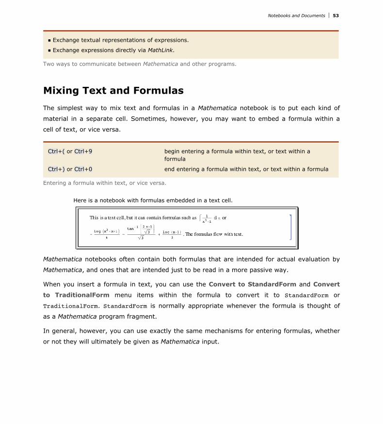
Mixing Text and Formulas

The simplest way to mix text and formulas in a Mathematica notebook is to put each kind of

material in a separate cell. Sometimes, however, you may want to embed a formula within a

cell of text, or vice versa.

Ctrl+( or Ctrl+9 begin entering a formula within text, or text within a formula

Ctrl+) or Ctrl+0 end entering a formula within text, or text within a formula

Entering a formula within text, or vice versa.

Here is a notebook with formulas embedded in a text cell.

Mathematica notebooks often contain both formulas that are intended for actual evaluation by

Mathematica, and ones that are intended just to be read in a more passive way.

When you insert a formula in text, you can use the Convert to StandardForm and Convert

to TraditionalForm menu items within the formula to convert it to StandardForm or

TraditionalForm. StandardForm is normally appropriate whenever the formula is thought of

as a Mathematica program fragment.

In general, however, you can use exactly the same mechanisms for entering formulas, whether

or not they will ultimately be given as Mathematica input.


You should realize, however, that to make the detailed typography of typical formulas look as

good as possible, Mathematica automatically does things such as inserting spaces around

certain operators. But these kinds of adjustments can potentially be inappropriate if you use

notation in very different ways from the ones Mathematica is expecting. In such cases, you may

have to make detailed typographical adjustments by hand.

Displaying and Printing Mathematica Notebooks

Depending on the purpose for which you are using a Mathematica notebook, you may want to

change its overall appearance. The front end allows you to specify independently the styles to

be used for display on the screen and for printing. Typically you can do this by choosing appropri-

ate items in the Format menu.

ScreenStyleEnvironment styles to be used for screen display

PrintingStyleEnvironment styles to be used for printed output

Working standard style definitions for screen display

Presentation style definitions for presentations

SlideShow style definitions for displaying presentation slides

Printout style definitions for printed output

Front end settings that define the global appearance of a notebook.

Here is a typical notebook as it appears in working form on the screen.


Here is a preview of how the notebook would appear when printed out.

Setting Up Hyperlinks

Insert Hyperlink menu item to make the selected object a hyperlink

Hyperlink@"uri"D generate as output a hyperlink with the label and destina -tion set as uri

Hyperlink@"label","uri"D generate as output a hyperlink with the label label and the destination uri

HyperlinkA9" file.nb",None=E generate as output a hyperlink to the specified notebook

Hyperlink@8" file.nb","tag"<D generate as output a hyperlink to the cell tagged as tag in the specified notebook

Methods for generating hyperlinks.

A hyperlink is a special kind of button which jumps to another part of a notebook when it is

pressed. Typically hyperlinks are indicated in Mathematica by blue text.

To set up a hyperlink, just select the text or other object that you want to be a hyperlink. Then

choose the menu item Insert Hyperlink and fill in the specification of where you want the

destination of the hyperlink to be.

The destination of a hyperlink can be any standard web address (URI). Hyperlinks can also

point to notebooks on the local file system, or even to specific cells inside those notebooks.

Hyperlinks which point to specific cells in notebooks use cell tags to identify the cells. If a particu -

lar cell tag is used for more than one cell in a given notebook, then the hyperlink will go to the

first instance of a cell with that cell tag.

A hyperlink can be generated in output by using the Mathematica command Hyperlink. These

hyperlinks can be copied and pasted into text or used in a larger interface being generated by

Mathematica.


A hyperlink can be generated in output by using the Mathematica command Hyperlink. These

hyperlinks can be copied and pasted into text or used in a larger interface being generated by

Mathematica.

This command generates a hyperlink to the web.

In[1]:= Hyperlink@"Wolfram Research, Inc.", "http:êêwww.wolfram.com"D

Out[1]= Wolfram Research, Inc.

Automatic Numbering

† Choose a cell style such as DisplayFormulaNumbered.

† Use the Insert Automatic Numbering menu item, with a counter name such as Section.

Two ways to set up automatic numbering in a Mathematica notebook.

Using the DisplayFormulaNumbered style

These cells are in DisplayFormulaNumbered style. DisplayFormulaNumbered style is available in stylesheets such as "Report".

Using the AutomaticNumbering menu item

The input for each cell here is exactly the same, but the cells contain an element that displays as a progressively larger number as one goes through the notebook.

Exposition in Mathematica Notebooks


Exposition in Mathematica Notebooks

Mathematica notebooks provide the basic technology that you need to be able to create a very

wide range of sophisticated interactive documents. But to get the best out of this technology

you need to develop an appropriate style of exposition.

Many people at first tend to use Mathematica notebooks either as simple worksheets containing

a sequence of input and output lines, or as onscreen versions of traditional books and other

printed material. But the most effective and productive uses of Mathematica notebooks tend to

lie at neither one of these extremes, and instead typically involve a fine-grained mixing of

Mathematica input and output with explanatory text. In most cases the single most important

factor in obtaining such fine-grained mixing is uniform use of the Mathematica language.

One might think that there would tend to be four kinds of material in a Mathematica notebook:

plain text, mathematical formulas, computer code, and interactive interfaces. But one of the

key ideas of Mathematica is to provide a single language that offers the best of both traditional

mathematical formulas and computer code.

In StandardForm, Mathematica expressions have the same kind of compactness and elegance

as traditional mathematical formulas. But unlike such formulas, Mathematica expressions are

set up in a completely consistent and uniform way. As a result, if you use Mathematica expres-

sions, then regardless of your subject matter, you never have to go back and reexplain your

basic notation: it is always just the notation of the Mathematica language. In addition, if you

set up your explanations in terms of Mathematica expressions, then a reader of your notebook

can immediately take what you have given, and actually execute it as Mathematica input.

If one has spent many years working with traditional mathematical notation, then it takes a

little time to get used to seeing mathematical facts presented as StandardForm Mathematica

expressions. Indeed, at first one often has a tendency to try to use TraditionalForm whenever

possible, perhaps with hidden tags to indicate its interpretation. But quite soon one tends to

evolve to a mixture of StandardForm and TraditionalForm. And in the end it becomes clear

that StandardForm alone is for most purposes the most effective form of presentation.

In traditional mathematical exposition, there are many tricks for replacing chunks of text by

fragments of formulas. In StandardForm many of these same tricks can be used. But the fact

that Mathematica expressions can represent not only mathematical objects but also procedures,

algorithms, graphics, and interfaces increases greatly the extent to which chunks of text can be

replaced by shorter and more precise material.


In traditional mathematical exposition, there are many tricks for replacing chunks of text by

that Mathematica expressions can represent not only mathematical objects but also procedures,

algorithms, graphics, and interfaces increases greatly the extent to which chunks of text can be

replaced by shorter and more precise material.

Named Characters

Mathematica provides systemwide support for a large number of special characters. Each charac -

ter has a name and a number of shortcut aliases. They are fully supported by the standard

Mathematica fonts.

Interpretation of Characters

The interpretations given here are those used in StandardForm and InputForm. Most of the

interpretations also work in TraditionalForm.

You can override the interpretations by giving your own rules for MakeExpression.

Letters and letter-like forms used in symbol names

Infix operators e.g. x⊕y

Prefix operators e.g. Ÿ x

Postfix operators e.g. x !

Matchfix operators e.g. Xx\

Compound operators e.g. Ÿ f „ x

Raw operators operator characters that can be typed on an ordinary keyboard

Spacing characters interpreted in the same way as an ordinary space

Structural elements characters used to specify structure; usually ignored in interpretation

Uninterpretable elements characters indicating missing information

Types of characters.

The precedences of operators are given in "Operator Input Forms".

Infix operators for which no grouping is specified in the listing are interpreted so that for exam-

ple x⊕y⊕z becomes CirclePlus@x, y, zD.

Naming Conventions


Naming Conventions

Characters that correspond to built-in Mathematica functions typically have names correspond-

ing to those functions. Other characters typically have names that are as generic as possible.

Characters with different names almost always look at least slightly different.

\@Capital…D uppercase form of a letter

\@Left…D and \@Right…D pieces of a matchfix operator (also arrows)

\@Raw…D a printable ASCII character

\@…IndicatorD a visual representation of a keyboard character

Some special classes of characters.

style Script, Gothic, etc.

variation Curly, Gray, etc.

case Capital, etc.

modifiers Not, Double, Nested, etc.

direction Left, Up, UpperRight, etc.

base A, Epsilon, Plus, etc.

diacritical mark Acute, Ring, etc.

Typical ordering of elements in character names.

Aliases

Mathematica supports both its own system of aliases, as well as aliases based on character

names in TeX and SGML or HTML. Except where they conflict, character names corresponding

to plain TeX, LaTeX and AMSTeX are all supported. Note that TeX and SGML or HTML aliases

are not given explicitly in the list of characters below.

Esc xxxEsc ordinary Mathematica alias

Esc îxxxEsc TeX alias

Esc & xxxEsc SGML or HTML alias

Types of aliases.


The following general conventions are used for all aliases:

† Characters that are alternatives to standard keyboard operators use these operators astheir aliases (e.g. Esc ->Esc for Ø, Esc &&Esc for fl).

† Most single-letter aliases stand for Greek letters.

† Capital-letter characters have aliases beginning with capital letters.

† When there is ambiguity in the assignment of aliases, a space is inserted at the beginningof the alias for the less common character (e.g. Esc ->Esc for î @RuleD and Esc â->Esc for î@RightArrowD).

† ! is inserted at the beginning of the alias for a Not character.

† TeX aliases begin with a backslash î.

† SGML aliases begin with an ampersand &.

† User-defined aliases conventionally begin with a dot or comma.

Font Matching

The special fonts provided with Mathematica include all the characters given in this listing.

Some of these characters also appear in certain ordinary text fonts.

When rendering text in a particular font, the Mathematica notebook front end will use all the

characters available in that font. It will use the special Mathematica fonts only for other charac-

ters.

A choice is made between Times-like, Helvetica-like (sans serif) and Courier-like (monospaced)

variants to achieve the best matching with the ordinary text font in use.


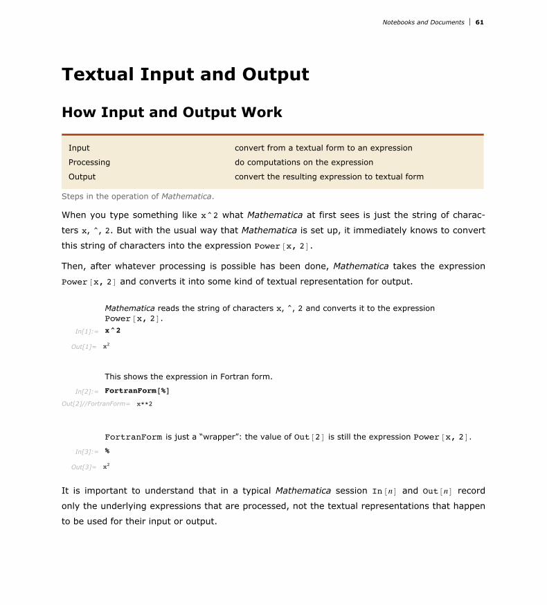
Textual Input and Output

How Input and Output Work

Input convert from a textual form to an expression

Processing do computations on the expression

Output convert the resulting expression to textual form

Steps in the operation of Mathematica.

When you type something like x^2 what Mathematica at first sees is just the string of charac-

ters x, ^, 2. But with the usual way that Mathematica is set up, it immediately knows to convert

this string of characters into the expression Power@x, 2D.

Then, after whatever processing is possible has been done, Mathematica takes the expression

Power@x, 2D and converts it into some kind of textual representation for output.

Mathematica reads the string of characters x, ^, 2 and converts it to the expression Power@x, 2D.

In[1]:= x^2

Out[1]= x2

This shows the expression in Fortran form.

In[2]:= FortranForm@%D

Out[2]//FortranForm= x**2

FortranForm is just a “wrapper”: the value of Out@2D is still the expression Power@x, 2D.

In[3]:= %

Out[3]= x2

It is important to understand that in a typical Mathematica session In@nD and Out@nD record

only the underlying expressions that are processed, not the textual representations that happen

to be used for their input or output.

If you explicitly request a particular kind of output, say by using TraditionalForm@exprD, then

what you get will be labeled with Out@nD êê TraditionalForm. This indicates that what you are

seeing is expr êê TraditionalForm, even though the value of Out@nD itself is just expr.


If you explicitly request a particular kind of output, say by using TraditionalForm@exprD, then

what you get will be labeled with Out@nD êê TraditionalForm. This indicates that what you are

seeing is expr êê TraditionalForm, even though the value of Out@nD itself is just expr.

Mathematica also allows you to specify globally that you want output to be displayed in a particu -

lar form. And if you do this, then the form will no longer be indicated explicitly in the label for

each line. But it is still the case that In@nD and Out@nD will record only underlying expressions,

not the textual representations used for their input and output.

This sets t to be an expression with FortranForm explicitly wrapped around it.

In[4]:= t = FortranForm@x^2 + y^2D

Out[4]//FortranForm= x**2 + y**2

The result on the previous line is just the expression.

In[5]:= %

Out[5]= x2 + y2

But t contains the FortranForm wrapper, and so is displayed in FortranForm .

In[6]:= t

Out[6]//FortranForm= x**2 + y**2

Wherever t appears, it is formatted in FortranForm .

In[7]:= 8t^2, 1 ê t<

Out[7]= :x ** 2 + y ** 22,1

x ** 2 + y ** 2>

The Representation of Textual Forms

Like everything else in Mathematica the textual forms of expressions can themselves be repre-

sented as expressions. Textual forms that consist of one-dimensional sequences of characters

can be represented directly as ordinary Mathematica strings. Textual forms that involve sub-

scripts, superscripts and other two-dimensional constructs, however, can be represented by

nested collections of two-dimensional boxes.


One-dimensional strings InputForm , FullForm , etc.

Two-dimensional boxes StandardForm , TraditionalForm , etc.

Typical representations of textual forms.

This generates the string corresponding to the textual representation of the expression in InputForm.

In[1]:= ToString@x^2 + y^3, InputFormD

Out[1]= x^2 + y^3

FullForm shows the string explicitly.

In[2]:= FullForm@%D

Out[2]//FullForm= "x^2 + y^3"

Here are the individual characters in the string.

In[3]:= Characters@%D

Out[3]= 8x, ^, 2, , +, , y, ^, 3<

Here is the box structure corresponding to the expression in StandardForm.

In[4]:= ToBoxes@x^2 + y^3, StandardFormD

Out[4]= RowBox@8SuperscriptBox@x, 2D, +, SuperscriptBox@y, 3D<D

Here is the InputForm of the box structure. In this form the structure is effectively represented by an ordinary string.

In[5]:= ToBoxes@x^2 + y^3, StandardFormD êê InputForm

Out[5]//InputForm= $x\^2 + y\^3$

If you use the notebook front end for Mathematica, then you can see the expression that corre-

sponds to the textual form of each cell by using the Show Expression menu item.

Here is a cell containing an expression in StandardForm.


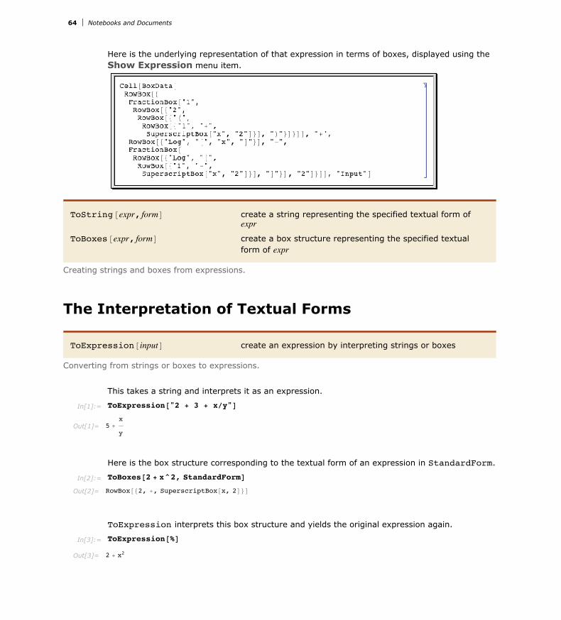
Here is the underlying representation of that expression in terms of boxes, displayed using the Show Expression menu item.

ToString@expr, formD create a string representing the specified textual form of expr

ToBoxes@expr, formD create a box structure representing the specified textual form of expr

Creating strings and boxes from expressions.

The Interpretation of Textual Forms

ToExpression@inputD create an expression by interpreting strings or boxes

Converting from strings or boxes to expressions.

This takes a string and interprets it as an expression.

In[1]:= ToExpression@"2 + 3 + xêy"D

Out[1]= 5 +x

y

Here is the box structure corresponding to the textual form of an expression in StandardForm.

In[2]:= ToBoxes@2 + x^2, StandardFormD

Out[2]= RowBox@82, +, SuperscriptBox@x, 2D<D

ToExpression interprets this box structure and yields the original expression again.

In[3]:= ToExpression@%D

Out[3]= 2 + x2

In any Mathematica session, Mathematica is always effectively using ToExpression to interpret

the textual form of your input as an actual expression to evaluate.


In any Mathematica session, Mathematica is always effectively using ToExpression to interpret

the textual form of your input as an actual expression to evaluate.

If you use the notebook front end for Mathematica, then the interpretation only takes place

when the contents of a cell are sent to the kernel, say for evaluation. This means that within a

notebook there is no need for the textual forms you set up to correspond to meaningful Mathe-

matica expressions; this is only necessary if you want to send these forms to the kernel.

FullForm explicit functional notation

InputForm one-dimensional notation

StandardForm two-dimensional notation

The hierarchy of forms for standard Mathematica input.

Here is an expression entered in FullForm.

In[4]:= Plus@1, Power@x, 2DD

Out[4]= 1 + x2

Here is the same expression entered in InputForm.

In[5]:= 1 + x^2

Out[5]= 1 + x2

And here is the expression entered in StandardForm.

In[6]:= 1 + x2

Out[6]= 1 + x2

Built into Mathematica is a collection of standard rules for use by ToExpression in converting

textual forms to expressions.

These rules define the grammar of Mathematica. They state, for example, that x + y should be

interpreted as Plus@x, yD, and that xy should be interpreted as Power@x, yD. If the input you

give is in FullForm, then the rules for interpretation are very straightforward: every expression

consists just of a head followed by a sequence of elements enclosed in brackets. The rules for

InputForm are slightly more sophisticated: they allow operators such as +, =, and ->, and

understand the meaning of expressions where these operators appear between operands.

StandardForm involves still more sophisticated rules, which allow operators and operands to be

arranged not just in a one-dimensional sequence, but in a full two-dimensional structure.

Mathematica is set up so that FullForm, InputForm and StandardForm form a strict hierarchy:

anything you can enter in FullForm will also work in InputForm, and anything you can enter in

InputForm will also work in StandardForm.


Mathematica is set up so that FullForm, InputForm and StandardForm form a strict hierarchy:

anything you can enter in FullForm will also work in InputForm, and anything you can enter in

InputForm will also work in StandardForm.

If you use a notebook front end for Mathematica, then you will typically want to use all the

features of StandardForm. If you use a text-based interface, however, then you will typically be

able to use only features of InputForm.

When you use StandardForm in a Mathematica notebook, you can enter directly two-dimen-

sional forms such as x2 or annotated graphics. But InputForm allows only one-dimensional

forms.

If you copy a StandardForm expression whose interpretation can be determined without evalua-

tion, then the expression will be pasted into external applications as InputForm. Otherwise, the

text is copied in a linear form that precisely represents the two-dimensional structure using î

! î H… îL. When you paste this linear form back into a Mathematica notebook, it will automati-

cally "snap" into two-dimensional form.

ToExpression@input, formD attempt to create an expression assuming that input is given in the specified textual form

Importing from other textual forms.

StandardForm and its subsets FullForm and InputForm provide precise ways to represent any

Mathematica expression in textual form. And given such a textual form, it is always possible to

convert it unambiguously to the expression it represents.

TraditionalForm is an example of a textual form intended primarily for output. It is possible to

take any Mathematica expression and display it in TraditionalForm. But TraditionalForm

does not have the precision of StandardForm, and as a result there is in general no unambigu-

ous way to go back from a TraditionalForm representation and get the expression it

represents.

Nevertheless, ToExpression@input, TraditionalFormD takes text in TraditionalForm and

attempts to interpret it as an expression.

This takes a string and interprets it as TraditionalForm input.

In[7]:= ToExpression@"fH6L", TraditionalFormD

Out[7]= f@6D

In StandardForm the same string would mean a product of terms.


In StandardForm the same string would mean a product of terms.

In[8]:= ToExpression@"fH6L", StandardFormD

Out[8]= 6 f

When TraditionalForm output is generated as the result of a computation, the actual collec-

tion of boxes that represent the output typically contains special Interpretation objects or

other specially tagged forms which specify how an expression can be reconstructed from the

TraditionalForm output.

The same is true of TraditionalForm that is obtained by explicit conversion from

StandardForm. But if you edit TraditionalForm extensively, or enter it from scratch, then

Mathematica will have to try to interpret it without the benefit of any additional embedded

information.

Short and Shallow Output

When you generate a very large output expression in Mathematica, you often do not want to

see the whole expression at once. Rather, you would first like to get an idea of the general

structure of the expression, and then, perhaps, go in and look at particular parts in more detail.

The functions Short and Shallow allow you to see “outlines” of large Mathematica expressions.

Short@exprD show a one-line outline of expr

Short@expr,nD show an n-line outline of expr

Shallow@exprD show the “top parts” of expr

Shallow@expr,8depth,length<D show the parts of expr to the specified depth and length

Showing outlines of expressions.

This generates a long expression. If the whole expression were printed out here, it would go on for 23 lines.

In[1]:= t = Expand@H1 + x + yL^12D;

This gives a one-line “outline” of t. The << >> indicates the number of terms omitted.

In[2]:= Short@tD

Out[2]//Short= 1 + 12 x + 66 x2 + 220 x3 + 495 x4 + á81à + 132 x y10 + 66 x2 y10 + 12 y11 + 12 x y11 + y12

When Mathematica generates output in a textual format such as OutputForm, it first effectively

writes the output in one long row. Then it looks at the width of text you have asked for, and it

chops the row of output into a sequence of separate “lines”. Each of the “lines” may of course

contain superscripts and built-up fractions, and so may take up more than one actual line on

your output device. When you specify a particular number of lines in Short, Mathematica takes

this to be the number of “logical lines” that you want, not the number of actual physical lines on

your particular output device.


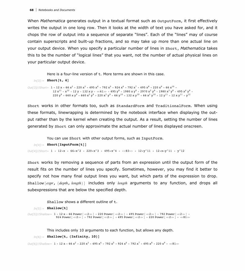
When Mathematica generates output in a textual format such as OutputForm, it first effectively

writes the output in one long row. Then it looks at the width of text you have asked for, and it

chops the row of output into a sequence of separate “lines”. Each of the “lines” may of course

contain superscripts and built-up fractions, and so may take up more than one actual line on

your output device. When you specify a particular number of lines in Short, Mathematica takes

this to be the number of “logical lines” that you want, not the number of actual physical lines on

your particular output device.

Here is a four-line version of t. More terms are shown in this case.

In[3]:= Short@t, 4D

Out[3]//Short= 1 + 12 x + 66 x2 + 220 x3 + 495 x4 + 792 x5 + 924 x6 + 792 x7 + 495 x8 + 220 x9 + 66 x10 +

12 x11 + x12 + 12 y + 132 x y + á61à + 495 y8 + 1980 x y8 + 2970 x2 y8 + 1980 x3 y8 + 495 x4 y8 +

220 y9 + 660 x y9 + 660 x2 y9 + 220 x3 y9 + 66 y10 + 132 x y10 + 66 x2 y10 + 12 y11 + 12 x y11 + y12

Short works in other formats too, such as StandardForm and TraditionalForm. When using

these formats, linewrapping is determined by the notebook interface when displaying the out-

put rather than by the kernel when creating the output. As a result, setting the number of lines

generated by Short can only approximate the actual number of lines displayed onscreen.

You can use Short with other output forms, such as InputForm.

In[4]:= Short@InputForm@tDD

Out[4]//Short= 1 + 12*x + 66*x^2 + 220*x^3 + 495*x^4 + <<83>> + 12*y^11 + 12*x*y^11 + y^12

Short works by removing a sequence of parts from an expression until the output form of the

result fits on the number of lines you specify. Sometimes, however, you may find it better to

specify not how many final output lines you want, but which parts of the expression to drop.

Shallow@expr, 8depth, length<D includes only length arguments to any function, and drops all

subexpressions that are below the specified depth.

Shallow shows a different outline of t.

In[5]:= Shallow@tD

Out[5]//Shallow= 1 + 12 x + 66 Power@á2àD + 220 Power@á2àD + 495 Power@á2àD + 792 Power@á2àD +924 Power@á2àD + 792 Power@á2àD + 495 Power@á2àD + 220 Power@á2àD + á81à

This includes only 10 arguments to each function, but allows any depth.

In[6]:= Shallow@t, 8Infinity, 10<D

Out[6]//Shallow= 1 + 12 x + 66 x2 + 220 x3 + 495 x4 + 792 x5 + 924 x6 + 792 x7 + 495 x8 + 220 x9 + á81à

Shallow is particularly useful when you want to drop parts in a uniform way throughout a

highly nested expression, such as a large list structure returned by Trace.


Shallow is particularly useful when you want to drop parts in a uniform way throughout a

highly nested expression, such as a large list structure returned by Trace.

Here is the recursive definition of the Fibonacci function.

In[7]:= fib@n_D := fib@n - 1D + fib@n - 2D; fib@0D = fib@1D = 1

Out[7]= 1

This generates a large list structure.

In[8]:= tr = Trace@fib@8DD;

You can use Shallow to see an outline of the structure.

In[9]:= Shallow@trD

Out[9]//Shallow= 8fib@á1àD, Plus@á2àD, 88á2à<, á1à, á1à, 8á7à<, 8á7à<, á1à, á1à<,88á2à<, á1à, á1à, 8á7à<, 8á7à<, á1à, á1à<, Plus@á2àD, 34<

Short gives you a less uniform outline, which can be more difficult to understand.

In[10]:= Short@tr, 4D

Out[10]//Short= 8fib@8D, fib@8 - 1D + fib@8 - 2D, 888 - 1, 7<, fib@7D, á3à, 13 + 8, 21<, 8á1à<, 21 + 13, 34<

When generated outputs in the notebook interface are exceedingly large, Mathematica automati-

cally applies Short to the output. This user interface enhancement prevents Mathematica from

spending a lot of time generating and formatting the printed output for an evaluation which

probably generated output you did not expect.

Typically, an assignment like this would have a semicolon at the end.

In[11]:= lst = RangeA106E

Out[11]=

A very large output was generated. Here is a sample of it:

81, 2, 3, 4, 5, 6, 7, 8, 9, 10, 11, 12, 13, 14, 15, 16, 17, 18, á999 964à,999983, 999984, 999985, 999986, 999987, 999988, 999989, 999990, 999991,999992, 999993, 999994, 999995, 999996, 999997, 999998, 999999, 1000000<

Show Less Show More Show Full Output Set Size Limit...

The buttons in the user interface allow you to control how much of the output you see. The size

threshold at which this behavior takes effect is determined by the byte count of the output

expression. That byte count can be set in the Preferences dialog of the notebook interface,

which is opened by the Set Size Limit button.

String-Oriented Output Formats


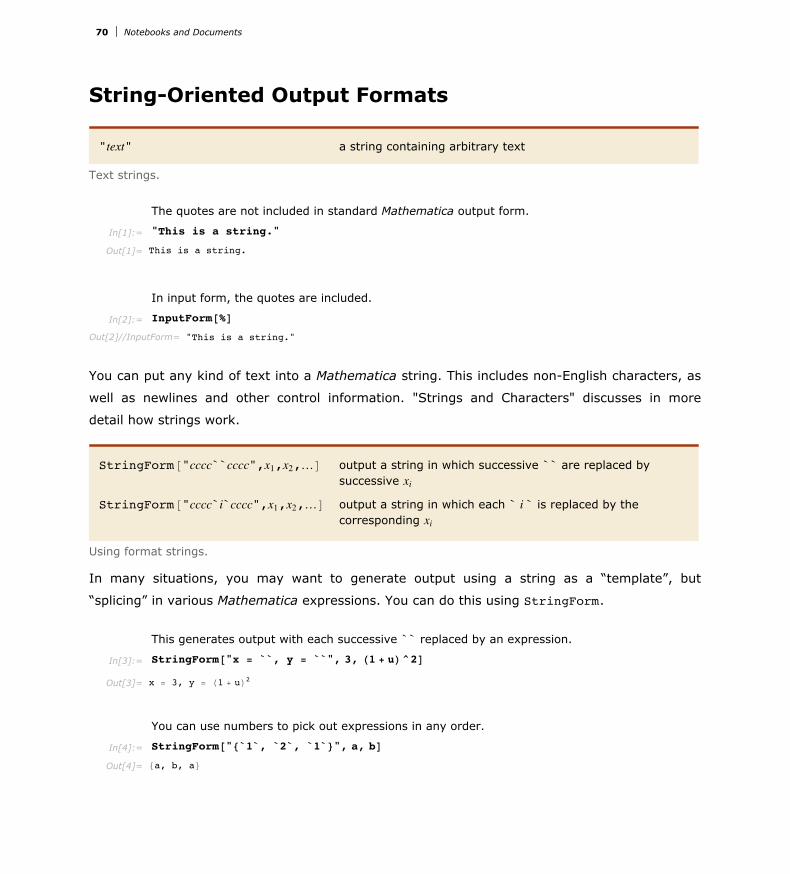
String-Oriented Output Formats

"text" a string containing arbitrary text

Text strings.

The quotes are not included in standard Mathematica output form.

In[1]:= "This is a string."

Out[1]= This is a string.

In input form, the quotes are included.

In[2]:= InputForm@%D

Out[2]//InputForm= "This is a string."

You can put any kind of text into a Mathematica string. This includes non-English characters, as

well as newlines and other control information. "Strings and Characters" discusses in more

detail how strings work.

StringForm@"cccc``cccc",x1,x2,…D output a string in which successive `` are replaced by successive xi

StringForm@"cccc`i`cccc",x1,x2,…D output a string in which each ` i ` is replaced by the corresponding xi

Using format strings.

In many situations, you may want to generate output using a string as a “template”, but

“splicing” in various Mathematica expressions. You can do this using StringForm.

This generates output with each successive `` replaced by an expression.

In[3]:= StringForm@"x = ``, y = ``", 3, H1 + uL^2D

Out[3]= x = 3, y = H1 + uL2

You can use numbers to pick out expressions in any order.

In[4]:= StringForm@"8`1`, `2`, `1`<", a, bD

Out[4]= 8a, b, a<

The string in StringForm acts somewhat like a “format directive” in the formatted output state-

ments of languages such as C and Fortran. You can determine how the expressions in

StringForm will be formatted by wrapping them with standard output format functions.


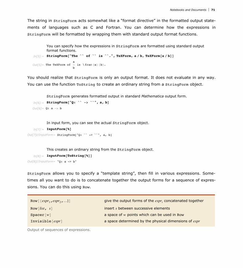
The string in StringForm acts somewhat like a “format directive” in the formatted output state-

ments of languages such as C and Fortran. You can determine how the expressions in

StringForm will be formatted by wrapping them with standard output format functions.

You can specify how the expressions in StringForm are formatted using standard output format functions.

In[5]:= StringForm@"The `` of `` is ``.", TeXForm, a ê b, TeXForm@a ê bDD

Out[5]= The TeXForm ofa

bis \frac 8a< 8b<.

You should realize that StringForm is only an output format. It does not evaluate in any way.

You can use the function ToString to create an ordinary string from a StringForm object.

StringForm generates formatted output in standard Mathematica output form.

In[6]:= StringForm@"Q: `` -> ``", a, bD

Out[6]= Q: a -> b

In input form, you can see the actual StringForm object.


Out[7]//InputForm= StringForm["Q: `` -> ``", a, b]

This creates an ordinary string from the StringForm object.

In[8]:= InputForm@ToString@%DD

Out[8]//InputForm= "Q: a -> b"

StringForm allows you to specify a “template string”, then fill in various expressions. Some-

times all you want to do is to concatenate together the output forms for a sequence of expres-

sions. You can do this using Row.

Row@8expr1,expr2,…<D give the output forms of the expri concatenated together

Row@list, sD insert s between successive elements

Spacer@wD a space of w points which can be used in Row

Invisible@exprD a space determined by the physical dimensions of expr

Output of sequences of expressions.


Row prints as a sequence of expressions concatenated together.

In[9]:= Row@8"@x = ", 56, "D"<D

Out[9]= @x = 56D

Row also works with typeset expressions.

In[10]:= Row@8"@y = ", Subscript@a, bD, "D"<D

Out[10]= @y = abD

Row can automatically insert any expression between the displayed elements.

In[11]:= Row@8a, b, c, d<, "õ"D

Out[11]= aõbõcõd

Spacer can be used to control the precise spacing between elements.

In[12]:= Row@8"x", Spacer@10D, "y"<D

Out[12]= x y

Column@8expr1,expr2,…<D a left-aligned column of objects

Column@list,alignmentD a column with a specified horizontal alignment (Left, Center or Right)

Column@list,alignment,sD a column with elements separated by s x-heights

Output of columns of expressions.

This arranges the two expressions in a column.

In[13]:= Column@8a + b, x^2<D

Out[13]=a + b

x2

Defer@exprD give the output form of expr, with expr maintained unevaluated

Interpretation@e,exprD give an output which displays as e, but evaluates as expr

Output of unevaluated expressions.

Using text strings and functions like Row, you can generate pieces of output that do not necessar -

ily correspond to valid Mathematica expressions. Sometimes, however, you want to generate

output that corresponds to a valid Mathematica expression, but only so long as the expression

is not evaluated. The function Defer maintains its argument unevaluated, but allows it to be

formatted in the standard Mathematica output form.


Using text strings and functions like Row, you can generate pieces of output that do not necessar-

output that corresponds to a valid Mathematica expression, but only so long as the expression

is not evaluated. The function Defer maintains its argument unevaluated, but allows it to be

formatted in the standard Mathematica output form.

Defer maintains 1 + 1 unevaluated.

In[14]:= Defer@1 + 1D

Out[14]= 1 + 1

The Defer prevents the actual assignment from being done.

In[15]:= Defer@x = 3D

Out[15]= x = 3

When the output of Defer is evaluated again, which might happen by modifying the output or

by using copy and paste, it will evaluate normally.

The following output was copied from the previous output cell into an input cell.

In[16]:= x = 3

Out[16]= 3

It is also possible to produce output whose appearance has no direct correlation to how it

evaluates by using Interpretation. This method is effectively used by Mathematica when

formatting some kinds of outputs where the most readable form does not correspond well to

the internal representation of the object. For example, Series always generates an

Interpretation object in its default output.

Although this output displays as y, it will evaluate as x.

In[17]:= Interpretation@y, xD

Out[17]= y

Copying and pasting the previous output will reference the value earlier assigned to x.

In[18]:= 2 y

Out[18]= 6


Output Formats for Numbers

ScientificForm@exprD print all numbers in scientific notation

EngineeringForm@exprD print all numbers in engineering notation (exponents divisible by 3)

AccountingForm@exprD print all numbers in standard accounting format

Output formats for numbers.

These numbers are given in the default output format. Large numbers are given in scientific notation.

In[1]:= 86.7^-4, 6.7^6, 6.7^8<

Out[1]= 90.00049625, 90458.4, 4.06068µ106=

This gives all numbers in scientific notation.

In[2]:= ScientificForm@%D

Out[2]//ScientificForm=

94.9625µ10-4, 9.04584µ104, 4.06068µ106=

This gives the numbers in engineering notation, with exponents arranged to be multiples of three.

In[3]:= EngineeringForm@%D

Out[3]//EngineeringForm=9496.25µ10-6, 90.4584µ103, 4.06068µ106=

In accounting form, negative numbers are given in parentheses, and scientific notation is never used.

In[4]:= [email protected], -6.7, 10.^7<D

Out[4]//AccountingForm=85.6, H6.7L, 10000000.<

NumberForm@expr,totD print at most tot digits of all approximate real numbers in expr

ScientificForm@expr,totD use scientific notation with at most tot digits

EngineeringForm@expr,totD use engineering notation with at most tot digits

Controlling the printed precision of real numbers.


Here is p9 to 30 decimal places.

In[5]:= N@Pi^9, 30D

Out[5]= 29809.0993334462116665094024012

This prints just 10 digits of p9.

In[6]:= NumberForm@%, 10D

Out[6]//NumberForm= 29809.09933

This gives 12 digits, in engineering notation.

In[7]:= EngineeringForm@%, 12D

Out[7]//EngineeringForm=

29.8090993334µ103

option name default valueDigitBlock Infinity maximum length of blocks of digits

between breaksNumberSeparator 8","," "< strings to insert at breaks between blocks

of digits to the left and right of a decimal point

NumberPoint "." string to use for a decimal pointNumberMultiplier "î@TimesD" string to use for the multiplication sign in

scientific notationNumberSigns 8"-",""< strings to use for signs of negative and

positive numbersNumberPadding 8"",""< strings to use for padding on the left and

rightSignPadding False whether to insert padding after the signNumberFormat Automatic function to generate final format of numberExponentFunction Automatic function to determine the exponent to use

Options for number formatting.

All the options in the table except the last one apply to both integers and approximate real

numbers.

All the options can be used in any of the functions NumberForm, ScientificForm ,

EngineeringForm and AccountingForm . In fact, you can in principle reproduce the behavior of

any one of these functions simply by giving appropriate option settings in one of the others.

The default option settings listed in the table are those for NumberForm.


Setting DigitBlock -> n breaks digits into blocks of length n.

In[8]:= NumberForm@30!, DigitBlock -> 3D

Out[8]//NumberForm= 265,252,859,812,191,058,636,308,480,000,000

You can specify any string to use as a separator between blocks of digits.

In[9]:= NumberForm@30!, DigitBlock -> 5, NumberSeparator -> " "D

Out[9]//NumberForm= 265 25285 98121 91058 63630 84800 00000

This gives an explicit plus sign for positive numbers, and uses » in place of a decimal point.

In[10]:= [email protected], -6.8<, NumberSigns -> 8"-", "+"<, NumberPoint -> "»"D

Out[10]//NumberForm=8+4»5, -6»8<

When Mathematica prints an approximate real number, it has to choose whether scientific

notation should be used, and if so, how many digits should appear to the left of the decimal

point. What Mathematica does is first to find out what the exponent would be if scientific nota-

tion were used, and one digit were given to the left of the decimal point. Then it takes this

exponent, and applies any function given as the setting for the option ExponentFunction. This

function should return the actual exponent to be used, or Null if scientific notation should not

be used.

The default is to use scientific notation for all numbers with exponents outside the range -5 to 5.

In[11]:= 88.^5, 11.^7, 13.^9<

Out[11]= 932768., 1.94872µ107, 1.06045µ1010=

This uses scientific notation only for numbers with exponents of 10 or more.

In[12]:= NumberForm@%, ExponentFunction -> HIf@-10 < Ò < 10, Null, ÒD &LD

Out[12]//NumberForm=

932768., 19487171., 1.06045µ1010=

This forces all exponents to be multiples of 3.

In[13]:= NumberForm@%, ExponentFunction -> H3 Quotient@Ò, 3D &LD

Out[13]//NumberForm=932.768µ103, 19.4872µ106, 10.6045µ109=

Having determined what the mantissa and exponent for a number should be, the final step is to

assemble these into the object to print. The option NumberFormat allows you to give an arbi-

trary function which specifies the print form for the number. The function takes as arguments

three strings: the mantissa, the base, and the exponent for the number. If there is no expo-

nent, it is given as "".


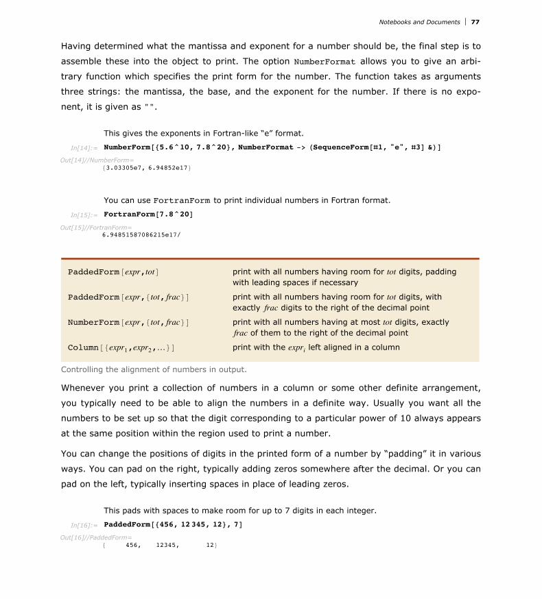
Having determined what the mantissa and exponent for a number should be, the final step is to

assemble these into the object to print. The option NumberFormat allows you to give an arbi-

trary function which specifies the print form for the number. The function takes as arguments

three strings: the mantissa, the base, and the exponent for the number. If there is no expo-

nent, it is given as "".

This gives the exponents in Fortran-like “e” format.

In[14]:= [email protected]^10, 7.8^20<, NumberFormat -> HSequenceForm@Ò1, "e", Ò3D &LD

Out[14]//NumberForm=83.03305e7, 6.94852e17<

You can use FortranForm to print individual numbers in Fortran format.

In[15]:= [email protected]^20D

Out[15]//FortranForm=6.94851587086215e17/

PaddedForm@expr,totD print with all numbers having room for tot digits, padding with leading spaces if necessary

PaddedForm@expr,8tot, frac<D print with all numbers having room for tot digits, with exactly frac digits to the right of the decimal point

NumberForm@expr,8tot, frac<D print with all numbers having at most tot digits, exactly frac of them to the right of the decimal point

Column@8expr1,expr2,…<D print with the expri left aligned in a column

Controlling the alignment of numbers in output.

Whenever you print a collection of numbers in a column or some other definite arrangement,

you typically need to be able to align the numbers in a definite way. Usually you want all the

numbers to be set up so that the digit corresponding to a particular power of 10 always appears

at the same position within the region used to print a number.

You can change the positions of digits in the printed form of a number by “padding” it in various

ways. You can pad on the right, typically adding zeros somewhere after the decimal. Or you can

pad on the left, typically inserting spaces in place of leading zeros.

This pads with spaces to make room for up to 7 digits in each integer.

In[16]:= PaddedForm@8456, 12345, 12<, 7D

Out[16]//PaddedForm=8 456, 12345, 12<

This creates a column of integers.


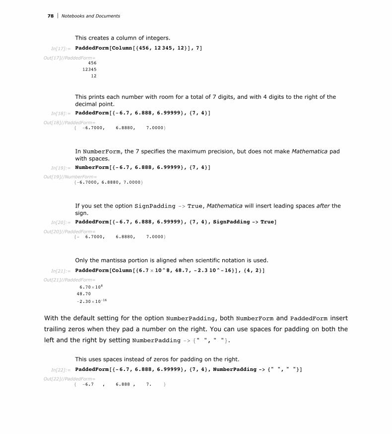
This creates a column of integers.

In[17]:= PaddedForm@Column@8456, 12345, 12<D, 7D

Out[17]//PaddedForm=456

1234512

This prints each number with room for a total of 7 digits, and with 4 digits to the right of the decimal point.

In[18]:= [email protected], 6.888, 6.99999<, 87, 4<D

Out[18]//PaddedForm=8 -6.7000, 6.8880, 7.0000<

In NumberForm, the 7 specifies the maximum precision, but does not make Mathematica pad with spaces.

In[19]:= [email protected], 6.888, 6.99999<, 87, 4<D

Out[19]//NumberForm=8-6.7000, 6.8880, 7.0000<

If you set the option SignPadding -> True, Mathematica will insert leading spaces after the sign.

In[20]:= [email protected], 6.888, 6.99999<, 87, 4<, SignPadding -> TrueD

Out[20]//PaddedForm=8- 6.7000, 6.8880, 7.0000<

Only the mantissa portion is aligned when scientific notation is used.

In[21]:= PaddedForm@[email protected] µ 10^8, 48.7, -2.3 10^-16<D, 84, 2<D

Out[21]//PaddedForm=

6.70µ108

48.70

-2.30µ10-16

With the default setting for the option NumberPadding, both NumberForm and PaddedForm insert

trailing zeros when they pad a number on the right. You can use spaces for padding on both the

left and the right by setting NumberPadding -> 8" ", " "<.

This uses spaces instead of zeros for padding on the right.

In[22]:= [email protected], 6.888, 6.99999<, 87, 4<, NumberPadding -> 8" ", " "<D

Out[22]//PaddedForm=8 -6.7 , 6.888 , 7. <


BaseForm@expr,bD print with all numbers given in base b

Printing numbers in other bases.

This prints a number in base 2.

In[23]:= BaseForm@2342424, 2D

Out[23]//BaseForm= 10001110111110000110002

In bases higher than 10, letters are used for the extra digits.

In[24]:= BaseForm@242345341, 16D

Out[24]//BaseForm= e71e57d16

BaseForm also works with approximate real numbers.

In[25]:= [email protected], 2D

Out[25]//BaseForm= 10.0100110011001100112

You can even use BaseForm for numbers printed in scientific notation.

In[26]:= [email protected] µ 10^8, 2D

Out[26]//BaseForm= 1.10110110101100001012 µ227

"Digits in Numbers" discusses how to enter numbers in arbitrary bases, and also how to get

lists of the digits in a number.

Tables and Matrices

Column@listD typeset as a column of elements

Grid@listD typeset as a grid of elements

TableForm@listD print in tabular form

Formatting lists as tables and matrices.

Here is a list.

In[1]:= Table@Hi + 45L^j, 8i, 3<, 8j, 3<D

Out[1]= 8846, 2116, 97336<, 847, 2209, 103823<, 848, 2304, 110592<<


Grid gives the list typeset in a tabular format.

In[2]:= Grid@%D

Out[2]=46 2116 9733647 2209 10382348 2304 110592

TableForm displays the list in a tabular format.

In[3]:= TableForm@%%D

Out[3]//TableForm=46 2116 9733647 2209 10382348 2304 110592

Grid and Column are wrappers which do not evaluate, but typeset their contents into appropri-

ate forms. They are typesetting constructs and require a front end to render correctly.

Column is a shorthand for a Grid with one column.

In[4]:= Column@Range@5DD

Out[4]=

12345

The FullForm of a Grid or Column demonstrates that the head is inert.

In[5]:= FullForm@%D

Out[5]//FullForm= Column@List@1, 2, 3, 4, 5DD

All of these wrappers can be used to present any kind of data, including graphical data.

In[6]:= Grid@88"disk", Graphics@Disk@D, ImageSize Ø 25D<,8"square", Graphics@Rectangle@D, ImageSize Ø 25D<<D

Out[6]=disk

square


PaddedFormAColumn@listD,totE print a column with all numbers padded to have room for tot digits

PaddedFormAGrid@listD,totE print a table with all numbers padded to have room for tot digits

PaddedFormAGrid@listD,8tot, frac<E put frac digits to the right of the decimal point in all approxi-mate real numbers

Printing tables of numbers.

Here is a list of numbers.

In[7]:= fac = 810!, 15!, 20!<

Out[7]= 83628800, 1307674368000, 2432902008176640000<

Column displays the list in a column.

In[8]:= Column@facD

Out[8]=362880013076743680002432902008176640000

This aligns the numbers by padding each one to leave room for up to 20 digits.

In[9]:= PaddedForm@Column@facD, 20D

Out[9]//PaddedForm=3628800

13076743680002432902008176640000

In this particular case, you could also align the numbers using the Alignment option.

In[10]:= Column@fac, Alignment -> 8Right<D

Out[10]=3628800

13076743680002432902008176640000

This lines up the numbers, padding each one to have room for 8 digits, with 5 digits to the right of the decimal point.

In[11]:= PaddedForm@[email protected], 6.888, 6.99999<D, 88, 5<D

Out[11]//PaddedForm=6.700006.888006.99999


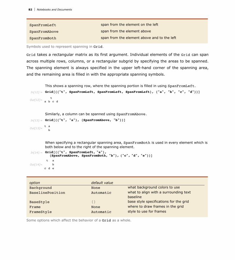
SpanFromLeft span from the element on the left

SpanFromAbove span from the element above

SpanFromBoth span from the element above and to the left

Symbols used to represent spanning in Grid.

Grid takes a rectangular matrix as its first argument. Individual elements of the Grid can span

across multiple rows, columns, or a rectangular subgrid by specifying the areas to be spanned.

The spanning element is always specified in the upper left-hand corner of the spanning area,

and the remaining area is filled in with the appropriate spanning symbols.

This shows a spanning row, where the spanning portion is filled in using SpanFromLeft.

In[12]:= Grid@88"t", SpanFromLeft, SpanFromLeft, SpanFromLeft<, 8"a", "b", "c", "d"<<D

Out[12]=t

a b c d

Similarly, a column can be spanned using SpanFromAbove.

In[13]:= Grid@88"t", "a"<, 8SpanFromAbove, "b"<<D

Out[13]=t a

b

When specifying a rectangular spanning area, SpanFromBoth is used in every element which is both below and to the right of the spanning element.

In[14]:= Grid@88"t", SpanFromLeft, "a"<,8SpanFromAbove, SpanFromBoth, "b"<, 8"c", "d", "e"<<D

Out[14]=t a

bc d e

option default valueBackground None what background colors to useBaselinePosition Automatic what to align with a surrounding text

baselineBaseStyle 8< base style specifications for the gridFrame None where to draw frames in the gridFrameStyle Automatic style to use for frames

Some options which affect the behavior of a Grid as a whole.


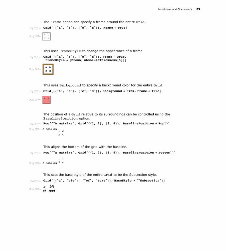
The Frame option can specify a frame around the entire Grid.

In[15]:= Grid@88"a", "b"<, 8"c", "d"<<, Frame Ø TrueD

Out[15]=a bc d

This uses FrameStyle to change the appearance of a frame.

In[16]:= Grid@88"a", "b"<, 8"c", "d"<<, Frame Ø True,FrameStyle Ø 8Brown, AbsoluteThickness@5D<D

Out[16]=a bc d

This uses Background to specify a background color for the entire Grid.

In[17]:= Grid@88"a", "b"<, 8"c", "d"<<, Background Ø Pink, Frame Ø TrueD

Out[17]=a bc d

The position of a Grid relative to its surroundings can be controlled using the BaselinePosition option.

In[18]:= Row@8"A matrix:", Grid@881, 2<, 83, 4<<, BaselinePosition Ø TopD<D

Out[18]= A matrix:1 23 4

This aligns the bottom of the grid with the baseline.

In[19]:= Row@8"A matrix:", Grid@881, 2<, 83, 4<<, BaselinePosition Ø BottomD<D

Out[19]= A matrix:

1 23 4

This sets the base style of the entire Grid to be the Subsection style.

In[20]:= Grid@88"a", "bit"<, 8"of", "text"<<, BaseStyle Ø 8"Subsection"<D

Out[20]=a bitof text


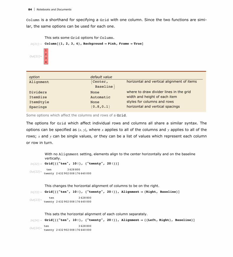
Column is a shorthand for specifying a Grid with one column. Since the two functions are simi-

lar, the same options can be used for each one.

This sets some Grid options for Column.

In[21]:= Column@81, 2, 3, 4<, Background Ø Pink, Frame Ø TrueD

Out[21]=

1234

option default valueAlignment 9Center,

Baseline=horizontal and vertical alignment of items

Dividers None where to draw divider lines in the gridItemSize Automatic width and height of each itemItemStyle None styles for columns and rowsSpacings 80.8,0.1< horizontal and vertical spacings

Some options which affect the columns and rows of a Grid.

The options for Grid which affect individual rows and columns all share a similar syntax. The

options can be specified as 8x, y<, where x applies to all of the columns and y applies to all of the

rows; x and y can be single values, or they can be a list of values which represent each column

or row in turn.

With no Alignment setting, elements align to the center horizontally and on the baseline vertically.

In[22]:= Grid@88"ten", 10!<, 8"twenty", 20!<<D

Out[22]=ten 3628800

twenty 2432902008176640000

This changes the horizontal alignment of columns to be on the right.

In[23]:= Grid@88"ten", 10!<, 8"twenty", 20!<<, Alignment Ø 8Right, Baseline<D

Out[23]=ten 3628800

twenty 2432902008176640000

This sets the horizontal alignment of each column separately.

In[24]:= Grid@88"ten", 10!<, 8"twenty", 20!<<, Alignment Ø 88Left, Right<, Baseline<D

Out[24]=ten 3628800twenty 2432902008176640000

When Background or ItemStyle options specify distinct settings for rows and columns, the

front end will attempt to combine the settings where the rows and columns overlap.


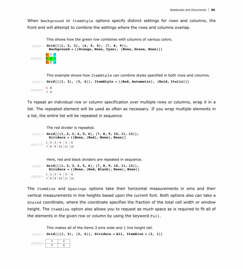
When Background or ItemStyle options specify distinct settings for rows and columns, the

front end will attempt to combine the settings where the rows and columns overlap.

This shows how the green row combines with columns of various colors.

In[25]:= Grid@881, 2, 3<, 84, 5, 6<, 87, 8, 9<<,Background Ø 88Orange, None, Cyan<, 8None, Green, None<<D

Out[25]=1 2 34 5 67 8 9

This example shows how ItemStyle can combine styles specified in both rows and columns.

In[26]:= Grid@881, 2<, 83, 4<<, ItemStyle Ø 88Red, Automatic<, 8Bold, Italic<<D

Out[26]=1 23 4

To repeat an individual row or column specification over multiple rows or columns, wrap it in a

list. The repeated element will be used as often as necessary. If you wrap multiple elements in

a list, the entire list will be repeated in sequence.

The red divider is repeated.

In[27]:= Grid@881, 2, 3, 4, 5, 6<, 87, 8, 9, 10, 11, 12<<,Dividers Ø 88None, 8Red<, None<, None<D

Out[27]=1 2 3 4 5 67 8 9 10 11 12

Here, red and black dividers are repeated in sequence.

In[28]:= Grid@881, 2, 3, 4, 5, 6<, 87, 8, 9, 10, 11, 12<<,Dividers Ø 88None, 8Red, Black<, None<, None<D

Out[28]=1 2 3 4 5 67 8 9 10 11 12

The ItemSize and Spacings options take their horizontal measurements in ems and their

vertical measurements in line heights based upon the current font. Both options also can take a

Scaled coordinate, where the coordinate specifies the fraction of the total cell width or window

height. The ItemSize option also allows you to request as much space as is required to fit all of

the elements in the given row or column by using the keyword Full.

This makes all of the items 3 ems wide and 1 line height tall.

In[29]:= Grid@881, 2<, 83, 4<<, Dividers Ø All, ItemSize Ø 83, 1<D

Out[29]=1 23 4

The same example in a new font size will show at a different size.


The same example in a new font size will show at a different size.

In[30]:= Style@Grid@881, 2<, 83, 4<<, Dividers Ø All, ItemSize Ø 83, 1<D, FontSize Ø 18D

Out[30]=1 23 4

The buttons in this example will always be sized to be a quarter of the width of the cell.

In[31]:= Grid@88Button@"Left button"D, Button@"Right button"D<<,ItemSize Ø [email protected]<<, Full<D

Out[31]= Left button Right button

The first and last settings for Spacings specify one-half of the top and bottom space.

In[32]:= Grid@881, 2<, 83, 4<<, Frame Ø True, Spacings Ø 881, 0, 1<, 81, 1, 1<<D

Out[32]=12

34

option default valueAlignment 9Center,

Baseline=horizontal and vertical alignment of items

Background None what background colors to useBaseStyle 8< base style specifications for the itemFrame None where to draw frames around the itemFrameStyle Automatic style to use for framesItemSize Automatic width and height of each item

Some options for Item.

Many of the settings which can be applied to entire rows and columns can also be applied

individually to the elements of a Grid or Column by using the Item wrapper. Item allows you to

change these settings at the granularity of a single item. Settings which are specified at the

Item level always override settings from the Grid or Column as a whole.

This sets item-specific options for the lower left-hand element.

In[33]:= Grid@881, 2<, 8Item@3, Background Ø LightGreen, Frame Ø TrueD, 4<<D

Out[33]=1 23 4


The Background setting for Item overrides the one for the Column.

In[34]:= Column@81, 2, Item@3, Background Ø PinkD<, Background Ø YellowD

Out[34]=123

Most of the options to Item take the same settings as their Grid counterparts. However, the

Alignment and ItemSize options, which allow complex row and column settings in Grid, take

only the 8horizontal, vertical< setting in Item.

This specifies a larger item area and how the text should be aligned within it.

In[35]:= Column@8Item@"Some aligned text", Frame Ø True,ItemSize Ø 815, 3<, Alignment Ø 8Center, Bottom<D, "caption"<D

Out[35]= Some aligned textcaption

The width value of the ItemSize option is used to determine line breaking.

In[36]:= Column@8Item@N@Pi, 20D, ItemSize Ø 810, 2<D, "digits of pi"<D

Out[36]=3.141592653589793Ö2385

digits of pi

The ItemSize here specifies a minimum height of 2 line heights, but the item is larger.

In[37]:= Column@8Item@N@Pi, 50D, ItemSize Ø 810, 2<D, "digits of pi"<D

Out[37]=

3.141592653589793Ö238462643383279Ö502884197169399Ö3751

digits of pi

Formatting Higher-Dimensional Data

Column supports one-dimensional data, and Grid supports two-dimensional data. To print

arrays with an arbitrary number of dimensions, you can use TableForm.

Here is the format for a 2×2 array of elements a@i, jD.

In[39]:= TableForm@Array@a, 82, 2<DD

Out[39]//TableForm=a@1, 1D a@1, 2Da@2, 1D a@2, 2D

Here is a 2×2×2 array.


Here is a 2×2×2 array.

In[40]:= TableForm@8Array@a, 82, 2<D, Array@b, 82, 2<D<D

Out[40]//TableForm=

a@1, 1Da@1, 2D

a@2, 1Da@2, 2D

b@1, 1Db@1, 2D

b@2, 1Db@2, 2D

And here is a 2×2×2×2 array.

In[41]:= TableForm@88Array@a, 82, 2<D, Array@b, 82, 2<D<, 8Array@c, 82, 2<D, Array@d, 82, 2<D<<D

Out[41]//TableForm=

a@1, 1D a@1, 2Da@2, 1D a@2, 2D

b@1, 1D b@1, 2Db@2, 1D b@2, 2D

c@1, 1D c@1, 2Dc@2, 1D c@2, 2D

d@1, 1D d@1, 2Dd@2, 1D d@2, 2D

In general, when you print an n-dimensional table, successive dimensions are alternately given

as columns and rows. By setting the option TableDirections -> 8dir1, dir2, …<, where the diri

are Column or Row, you can specify explicitly which way each dimension should be given. By

default, the option is effectively set to 8Column, Row, Column, Row, …<.

The option TableDirections allows you to specify explicitly how each dimension in a multidi- mensional table should be given.

In[42]:= TableForm@8Array@a, 82, 2<D, Array@b, 82, 2<D<,TableDirections -> 8Row, Row, Column<D

Out[42]//TableForm=a@1, 1Da@1, 2D

a@2, 1Da@2, 2D

b@1, 1Db@1, 2D

b@2, 1Db@2, 2D

TableForm can handle arbitrary “ragged” arrays. It leaves blanks wherever there are no ele-

ments supplied.

TableForm can handle “ragged” arrays.

In[43]:= TableForm@88a, a, a<, 8b, b<<D

Out[43]//TableForm=a a ab b

You can include objects that behave as “subtables”.

In[44]:= TableForm@88a, 88p, q<, 8r, s<<, a, a<, 88x, y<, b, b<<D

Out[44]//TableForm=a p q

r s a a

xy b b


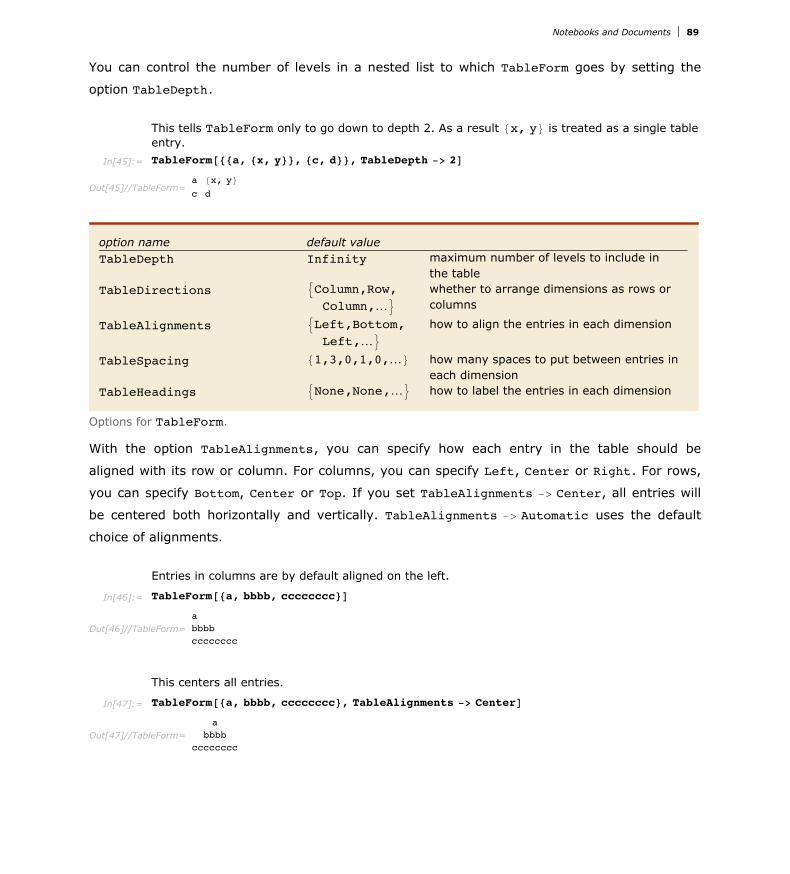
You can control the number of levels in a nested list to which TableForm goes by setting the

option TableDepth.

This tells TableForm only to go down to depth 2. As a result 8x, y< is treated as a single table entry.

In[45]:= TableForm@88a, 8x, y<<, 8c, d<<, TableDepth -> 2D

Out[45]//TableForm=a 8x, y<c d

option name default valueTableDepth Infinity maximum number of levels to include in

the tableTableDirections 9Column,Row,

Column,…=

whether to arrange dimensions as rows or columns

TableAlignments 9Left,Bottom,Left,…=

how to align the entries in each dimension

TableSpacing 81,3,0,1,0,…< how many spaces to put between entries in each dimension

TableHeadings 9None,None,…= how to label the entries in each dimension

Options for TableForm.

With the option TableAlignments, you can specify how each entry in the table should be

aligned with its row or column. For columns, you can specify Left, Center or Right. For rows,

you can specify Bottom, Center or Top. If you set TableAlignments -> Center, all entries will

be centered both horizontally and vertically. TableAlignments -> Automatic uses the default

choice of alignments.

Entries in columns are by default aligned on the left.

In[46]:= TableForm@8a, bbbb, cccccccc<D

Out[46]//TableForm=abbbbcccccccc

This centers all entries.

In[47]:= TableForm@8a, bbbb, cccccccc<, TableAlignments -> CenterD

Out[47]//TableForm=a

bbbbcccccccc


You can use the option TableSpacing to specify how much horizontal space there should be

between successive columns, or how much vertical space there should be between successive

rows. A setting of 0 specifies that successive objects should abut.

This leaves 6 spaces between the entries in each row, and no space between successive rows.

In[48]:= TableForm@88a, b<, 8ccc, d<<, TableSpacing -> 80, 6<D

Out[48]//TableForm= a bccc d

None no labels in any dimension

Automatic successive integer labels in each dimension

88lab11,lab12,…<,…< explicit labels

Settings for the option TableHeadings.

This puts integer labels in a 2×2×2 array.

In[49]:= TableForm@Array@a, 82, 2, 2<D, TableHeadings -> AutomaticD

Out[49]//TableForm=

1 2

11 a@1, 1, 1D2 a@1, 1, 2D

1 a@1, 2, 1D2 a@1, 2, 2D

21 a@2, 1, 1D2 a@2, 1, 2D

1 a@2, 2, 1D2 a@2, 2, 2D

This gives a table in which the rows are labeled by integers, and the columns by a list of strings.

In[50]:= TableForm@88a, b, c<, 8ap, bp, cp<<,TableHeadings -> 8Automatic, 8"first", "middle", "last"<<D

Out[50]//TableForm=first middle last

1 a b c2 ap bp cp

This labels the rows but not the columns. TableForm automatically drops the third label since there is no corresponding row.

In[51]:= TableForm@882, 3, 4<, 85, 6, 1<<,TableHeadings -> 88"row a", "row b", "row c"<, None<D

Out[51]//TableForm=row a 2 3 4row b 5 6 1


Styles and Fonts in Output

Style@expr,optionsD print with the specified style options

Style@expr,"style"D print with the specified cell style

Specifying output styles.

The second x2 is here shown in boldface.

In[1]:= 8x^2, Style@x^2, FontWeight -> "Bold"D<

Out[1]= 9x2, x2=

This shows the word text in font sizes from 10 to 20 points.

In[2]:= Table@Style@"text", FontSize -> sD, 8s, 10, 20<D

Out[2]= :text, text, text, text, text, text, text, text, text, text, text>

This shows the text in the Helvetica font.

In[3]:= Style@"some text", FontFamily -> "Helvetica"D

Out[3]= some text

Style allows an abbreviated form of some options. For options such as FontSize, FontWeight,

FontSlant and FontColor, you can include merely the setting of the option.

Options are specified here in a short form.

In[4]:= Style@"text", 20, ItalicD

Out[4]= text

option typical setting(s)FontSize 12 size of characters in printer's pointsFontWeight "Plain" or "Bold" weight of charactersFontSlant "Plain" or "Italic" slant of charactersFontFamily "Courier" ,

"Times" , "Helvetica"font family

FontColor GrayLevel@0D color of charactersBackground GrayLevel@1D background color for characters

A few options that can be used in Style.

If you use the notebook front end for Mathematica, then each piece of output that is generated

will by default be in the style of the cell in which the output appears. By using

Style@expr, "style"D however, you can tell Mathematica to output a particular expression in a

different style.


If you use the notebook front end for Mathematica, then each piece of output that is generated

will by default be in the style of the cell in which the output appears. By using

Style@expr, "style"D however, you can tell Mathematica to output a particular expression in a

different style.

Here is an expression output in the style normally used for section headings.

In[5]:= Style@x^2 + y^2, "Section"D

Out[5]= x2 + y2

"Cells as Mathematica Expressions" describes in more detail how cell styles work. By using

Style@expr, "style", optionsD you can generate output that is in a particular style, but with cer-

tain options modified.

Representing Textual Forms by Boxes

All textual and graphical forms in Mathematica are ultimately represented in terms of nested

collections of boxes. Typically the elements of these boxes correspond to objects that are to be

placed at definite relative positions in two dimensions.

Here are the boxes corresponding to the expression a + b.

In[1]:= ToBoxes@a + bD

Out[1]= RowBox@8a, +, b<D

DisplayForm shows how these boxes would be displayed.

In[2]:= DisplayForm@%D

Out[2]//DisplayForm= a + b

DisplayForm@boxesD show boxes as they would be displayed

Showing the displayed form of boxes.

This displays three strings in a row.

In[3]:= RowBox@8"a", "+", "b"<D êê DisplayForm

Out[3]//DisplayForm= a + b


This displays one string as a subscript of another.

In[4]:= SubscriptBox@"a", "i"D êê DisplayForm

Out[4]//DisplayForm= ai

This puts two subscript boxes in a row.

In[5]:= RowBox@8SubscriptBox@"a", "1"D, SubscriptBox@"b", "2"D<D êê DisplayForm

Out[5]//DisplayForm= a1 b2

"text" literal text

RowBox@8a,b,…<D a row of boxes or strings a, b, …GridBox@88a1,b1,…<,8a2,b2,…<,…<D

a grid of boxes

a1 b1 …a2 b2 …ª ª

SubscriptBox@a,bD subscript ab

SuperscriptBox@a,bD superscript ab

SubsuperscriptBox@a,b,cD subscript and superscript abc

UnderscriptBox@a,bD underscript ab

OverscriptBox@a,bD overscript ab

UnderoverscriptBox@a,b,cD underscript and overscript ab

c

FractionBox@a,bD fraction ab

SqrtBox@aD square root a

RadicalBox@a,bD bth root ab

Some basic box types.

This nests a fraction inside a radical.

In[6]:= RadicalBox@FractionBox@x, yD, nD êê DisplayForm

Out[6]//DisplayForm= x

yn


This puts a superscript on a subscripted object.

In[7]:= SuperscriptBox@SubscriptBox@a, bD, cD êê DisplayForm

Out[7]//DisplayForm= abc

This puts both a subscript and a superscript on the same object.

In[8]:= SubsuperscriptBox@a, b, cD êê DisplayForm

Out[8]//DisplayForm= abc

FrameBox@boxD render box with a frame drawn around it

GridBoxAlist,RowLines->TrueE put lines between rows in a GridBox

GridBoxAlist,ColumnLines->TrueE put lines between columns

GridBoxAlist,RowLines->9True,False=E

put a line below the first row, but not subsequent ones

Inserting frames and grid lines.

This shows a fraction with a frame drawn around it.

In[9]:= FrameBox@FractionBox@"x", "y"DD êê DisplayForm


y

This puts lines between rows and columns of an array.

In[10]:= GridBox@Table@i + j, 8i, 3<, 8j, 3<D,RowLines -> True, ColumnLines -> TrueD êê DisplayForm

Out[10]//DisplayForm= 2 3 43 4 54 5 6

And this also puts a frame around the outside.

In[11]:= FrameBox@%D êê DisplayForm

Out[11]//DisplayForm=

2 3 43 4 54 5 6


StyleBox@boxes,optionsD render boxes with the specified option settings

StyleBox@boxes,"style"D render boxes in the specified style

Modifying the appearance of boxes.

StyleBox takes the same options as Style. The difference is that Style is a high-level function

that applies to an expression to determine how it will be displayed, while StyleBox is the corre-

sponding low-level function in the underlying box structure.

This shows the string "name" in italics.

In[12]:= StyleBox@"name", FontSlant -> "Italic"D êê DisplayForm

Out[12]//DisplayForm= name

This shows "name" in the style used for section headings in your current notebook.

In[13]:= StyleBox@"name", "Section"D êê DisplayForm


name

This uses section heading style, but with characters shown in gray.

In[14]:= StyleBox@"name", "Section", FontColor -> [email protected] êê DisplayForm


name

If you use a notebook front end for Mathematica, then you will be able to change the style and

appearance of what you see on the screen directly by using menu items. Internally, however,

these changes will still be recorded by the insertion of appropriate StyleBox objects.

FormBox@boxes, formD interpret boxes using rules associated with the specified form

InterpretationBox@boxes,exprD interpret boxes as representing the expression expr

TagBox@boxes,tagD use tag to guide the interpretation of boxes

ErrorBox@boxesD indicate an error and do not attempt further interpretation of boxes

Controlling the interpretation of boxes.


This prints as x with a superscript.

In[15]:= SuperscriptBox@"x", "2"D êê DisplayForm

Out[15]//DisplayForm= x2

It is normally interpreted as a power.

In[16]:= ToExpression@%D êê InputForm

Out[16]//InputForm= x^2

This again prints as x with a superscript.

In[17]:= InterpretationBox@SuperscriptBox@"x", "2"D, vec@x, 2DD êê DisplayForm


x2

But now it is interpreted as vec@x, 2D, following the specification given in the InterpretationBox.

In[18]:= ToExpression@%D êê InputForm

Out[18]//InputForm= vec[x, 2]

If you edit the boxes given in an InterpretationBox, then there is no guarantee that the

interpretation specified by the interpretation box will still be correct. As a result, Mathematica

provides various options that allow you to control the selection and editing of

InterpretationBox objects.

option default valueEditable Automatic whether to allow the contents to be editedSelectable True whether to allow the contents to be selectedDeletable True whether to allow the box to be deletedDeletionWarning False whether to issue a warning if the box is

deletedBoxAutoDelete False whether to strip the box if its contents are

modifiedStripWrapperBoxes False whether to remove StyleBox etc. from

within boxes in TagBox@boxes, …D

Options for InterpretationBox and related boxes.

TagBox objects are used to store information that will not be displayed but which can neverthe-

less be used by the rules that interpret boxes. Typically the tag in TagBox@boxes, tagD is a symbol

which gives the head of the expression corresponding to boxes. If you edit only the arguments of

this expression then there is a good chance that the interpretation specified by the TagBox will

still be appropriate. As a result, Editable -> True is effectively the default setting for a

TagBox.


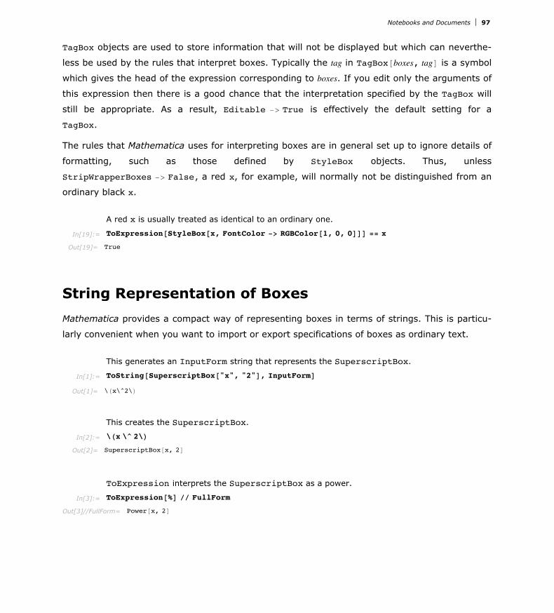
TagBox objects are used to store information that will not be displayed but which can neverthe-

less be used by the rules that interpret boxes. Typically the tag in TagBox@boxes, tagD is a symbol

which gives the head of the expression corresponding to boxes. If you edit only the arguments of

this expression then there is a good chance that the interpretation specified by the TagBox will

still be appropriate. As a result, Editable -> True is effectively the default setting for a

TagBox.

The rules that Mathematica uses for interpreting boxes are in general set up to ignore details of

formatting, such as those defined by StyleBox objects. Thus, unless

StripWrapperBoxes -> False, a red x, for example, will normally not be distinguished from an

ordinary black x.

A red x is usually treated as identical to an ordinary one.

In[19]:= ToExpression@StyleBox@x, FontColor -> RGBColor@1, 0, 0DDD == x

Out[19]= True

String Representation of Boxes

Mathematica provides a compact way of representing boxes in terms of strings. This is particu-

larly convenient when you want to import or export specifications of boxes as ordinary text.

This generates an InputForm string that represents the SuperscriptBox.

In[1]:= ToString@SuperscriptBox@"x", "2"D, InputFormD

Out[1]= \Hx\^2\L

This creates the SuperscriptBox.

In[2]:= \Hx \^ 2\L

Out[2]= SuperscriptBox@x, 2D

ToExpression interprets the SuperscriptBox as a power.

In[3]:= ToExpression@%D êê FullForm

Out[3]//FullForm= Power@x, 2D


It is important to distinguish between forms that represent just raw boxes, and forms that

represent the meaning of the boxes.

This corresponds to a raw SuperscriptBox.

In[4]:= \Hx \^ 2\L

Out[4]= SuperscriptBox@x, 2D

This corresponds to the power that the SuperscriptBox represents.

In[5]:= \!\Hx \^ 2\L

Out[5]= x2

The expression generated here is a power.

In[6]:= FullForm@\!\Hx \^ 2\LD

Out[6]//FullForm= Power@x, 2D

îHinputîL raw boxes

î!îHinputîL the meaning of the boxes

Distinguishing raw boxes from the expressions they represent.

If you copy the contents of a StandardForm cell into another program, such as a text editor,

Mathematica will generate a î ! î H… îL form where necessary. This is done so that if you

subsequently paste the form back into Mathematica, the original contents of the StandardForm

cell will automatically be re-created. Without the î !, only the raw boxes corresponding to

these contents would be obtained.

With default settings for options, î ! î H… îL forms pasted into Mathematica notebooks are

automatically displayed in two-dimensional form.

"îHinputîL" a raw character string

"î!îHinputîL" a string containing boxes

Embedding two-dimensional box structures in strings.

Mathematica will usually treat a î H… îL form that appears within a string just like any other

sequence of characters. But by inserting a î ! you can tell Mathematica instead to treat this

form like the boxes it represents. In this way you can therefore embed box structures within

ordinary character strings.

Mathematica treats this as an ordinary character string.


Mathematica treats this as an ordinary character string.

In[7]:= "\H x \^ 2 \L"

Out[7]= \H x \^ 2 \L

The ! î tells Mathematica that this string contains boxes.

In[8]:= "\!\H x \^ 2 \L"

Out[8]= x2

You can mix boxes with ordinary text.

In[9]:= "box 1: \!\Hx\^2\L; box 2: \!\Hy\^3\L"

Out[9]= box 1: x2; box 2: y3

îHbox1,box2,…îL RowBox@box1,box2,…D

box1î^box2 SuperscriptBox@box1,box2D

box1ï_ box2 SubscriptBox@box1,box2D

box1ï_ box2î% box3 SubsuperscriptBox@box1,box2,box3D

box1î& box2 OverscriptBox@box1,box2D

box1î+box2 UnderscriptBox@box1,box2D

box1î+box2î% box3 UnderoverscriptBox@box1,box2,box3D

box1îêbox2 FractionBox@box1,box2D

îübox SqrtBox@boxD

\übox1\%box2 RadicalBox@box1,box2D

formî` box FormBox@box, formD

\*input construct boxes from input

Input forms for boxes.

Mathematica requires that any input forms you give for boxes be enclosed within î H and î L.

But within these outermost î H and î L you can use additional î H and î L to specify grouping.

Here ordinary parentheses are used to indicate grouping.

In[10]:= \Hx \ê Hy + zL\L êê DisplayForm


Hy + zL


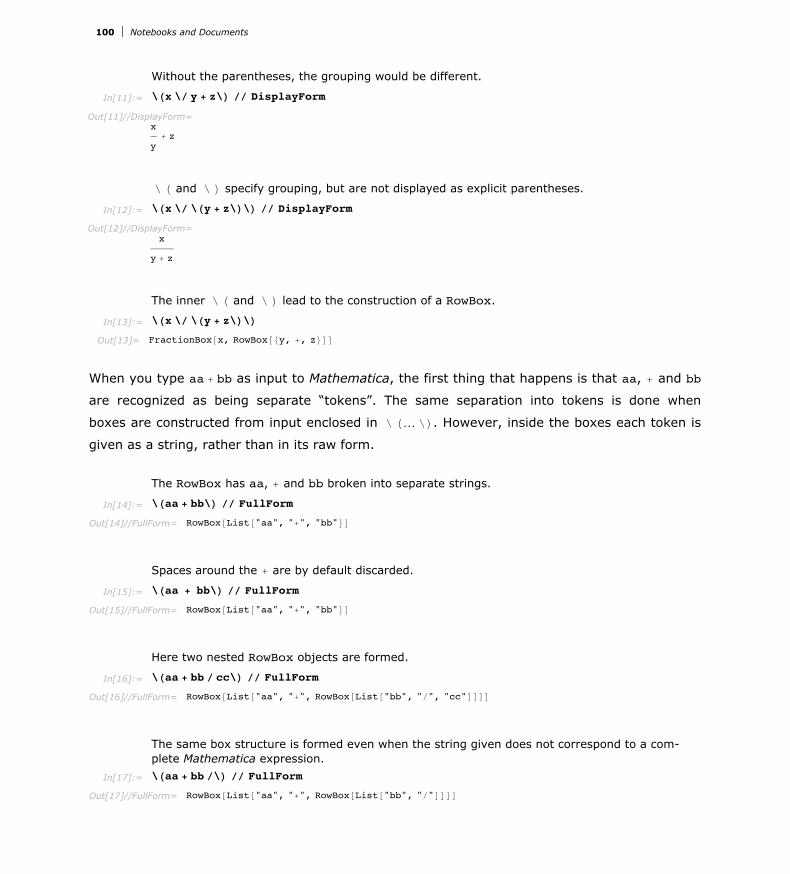
Without the parentheses, the grouping would be different.

In[11]:= \Hx \ê y + z\L êê DisplayForm


y+ z

î H and î L specify grouping, but are not displayed as explicit parentheses.

In[12]:= \Hx \ê \Hy + z\L\L êê DisplayForm


y + z

The inner î H and î L lead to the construction of a RowBox.

In[13]:= \Hx \ê \Hy + z\L\L

Out[13]= FractionBox@x, RowBox@8y, +, z<DD

When you type aa + bb as input to Mathematica, the first thing that happens is that aa, + and bb

are recognized as being separate “tokens”. The same separation into tokens is done when

boxes are constructed from input enclosed in î H… îL. However, inside the boxes each token is

given as a string, rather than in its raw form.

The RowBox has aa, + and bb broken into separate strings.

In[14]:= \Haa + bb\L êê FullForm

Out[14]//FullForm= RowBox@List@"aa", "+", "bb"DD

Spaces around the + are by default discarded.

In[15]:= \Haa + bb\L êê FullForm

Out[15]//FullForm= RowBox@List@"aa", "+", "bb"DD

Here two nested RowBox objects are formed.

In[16]:= \Haa + bb ê cc\L êê FullForm

Out[16]//FullForm= RowBox@List@"aa", "+", RowBox@List@"bb", "ê", "cc"DDDD

The same box structure is formed even when the string given does not correspond to a complete Mathematica expression.

In[17]:= \Haa + bb ê\L êê FullForm

Out[17]//FullForm= RowBox@List@"aa", "+", RowBox@List@"bb", "ê"DDDD

Within î H… îL sequences, you can set up certain kinds of boxes by using backslash notations

such as î ^ and î ü. But for other kinds of boxes, you need to give ordinary Mathematica

input, prefaced by î *.


Within î H… îL sequences, you can set up certain kinds of boxes by using backslash notations

such as î ^ and î ü. But for other kinds of boxes, you need to give ordinary Mathematica

input, prefaced by î *.

This constructs a GridBox.

In[18]:= \H\*GridBox@88"a", "b"<, 8"c", "d"<<D\L êê DisplayForm

Out[18]//DisplayForm= a bc d

This constructs a StyleBox.

In[19]:= \H\*StyleBox@"text", FontWeight -> "Bold"D\L êê DisplayForm

Out[19]//DisplayForm= text

î * in effect acts like an escape: it allows you to enter ordinary Mathematica syntax even

within a î H… îL sequence. Note that the input you give after a î * can itself in turn contain

î H… îL sequences.

You can alternate nested î * and î H… îL. Explicit quotes are needed outside of î H… îL.

In[20]:= \Hx + \*GridBox@88"a", "b"<,8\Hc \^ 2\L, \Hd \ê \*GridBox@88"x", "y"<, 8"x", "y"<<D\L<<D\L êê DisplayForm


x +

a b

c2 dx yx y

î!îHinputîL interpret input in the current form

î!îH formî`inputîL interpret input using the specified form

Controlling the way input is interpreted.

In a StandardForm cell, this will be interpreted in StandardForm, yielding a product.

In[21]:= \!\Hc H1 + xL\L

Out[21]= c H1 + xL

The backslash backquote sequence tells Mathematica to interpret this in TraditionalForm.

In[22]:= \!\HTraditionalForm \` c H1 + xL\L

Out[22]= c@1 + xD

When you copy the contents of a cell from a notebook into a program such as a text editor, no

explicit backslash backquote sequence is usually included. But if you expect to paste what you

get back into a cell of a different type from the one it came from, then you will typically need to

include a backslash backquote sequence in order to ensure that everything is interpreted

correctly.


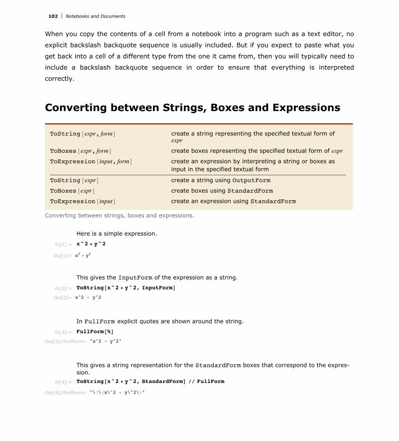
When you copy the contents of a cell from a notebook into a program such as a text editor, no

explicit backslash backquote sequence is usually included. But if you expect to paste what you

get back into a cell of a different type from the one it came from, then you will typically need to

include a backslash backquote sequence in order to ensure that everything is interpreted

correctly.

Converting between Strings, Boxes and Expressions

ToString@expr, formD create a string representing the specified textual form of expr

ToBoxes@expr, formD create boxes representing the specified textual form of expr

ToExpression@input, formD create an expression by interpreting a string or boxes as input in the specified textual form

ToString@exprD create a string using OutputForm

ToBoxes@exprD create boxes using StandardForm

ToExpression@inputD create an expression using StandardForm

Converting between strings, boxes and expressions.

Here is a simple expression.

In[1]:= x^2 + y^2

Out[1]= x2 + y2

This gives the InputForm of the expression as a string.

In[2]:= ToString@x^2 + y^2, InputFormD

Out[2]= x^2 + y^2

In FullForm explicit quotes are shown around the string.

In[3]:= FullForm@%D

Out[3]//FullForm= "x^2 + y^2"

This gives a string representation for the StandardForm boxes that correspond to the expression.

In[4]:= ToString@x^2 + y^2, StandardFormD êê FullForm

Out[4]//FullForm= "\!\Hx\^2 + y\^2\L"


ToBoxes yields the boxes themselves.

In[5]:= ToBoxes@x^2 + y^2, StandardFormD

Out[5]= RowBox@8SuperscriptBox@x, 2D, +, SuperscriptBox@y, 2D<D

In generating data for files and external programs, it is sometimes necessary to produce two-

dimensional forms which use only ordinary keyboard characters. You can do this using

OutputForm.

This produces a string which gives a two-dimensional rendering of the expression, using only ordinary keyboard characters.

In[6]:= ToString@x^2 + y^2, OutputFormD

Out[6]= 2 2x + y

The string consists of two lines, separated by an explicit î n newline.

In[7]:= FullForm@%D

Out[7]//FullForm= " 2 2\nx + y"

The string looks right only in a monospaced font.

In[8]:= Style@%, FontFamily -> "Times"D

Out[8]= 2 2x + y

If you operate only with one-dimensional structures, you can effectively use ToString to do

string manipulation with formatting functions.

This generates a string corresponding to the OutputForm of StringForm.

In[9]:= ToString@StringForm@"``^10 = ``", 4, 4^10DD êê InputForm

Out[9]//InputForm= "4^10 = 1048576"

InputForm strings corresponding to keyboard input

StandardForm strings or boxes corresponding to standard two-dimen -sional input (default)

TraditionalForm strings or boxes mimicking traditional mathematical notation

Some forms handled by ToExpression.


This creates an expression from an InputForm string.

In[10]:= ToExpression@"x^2 + y^2"D

Out[10]= x2 + y2

This creates the same expression from StandardForm boxes.

In[11]:= ToExpression@RowBox@8SuperscriptBox@"x", "2"D, "+", SuperscriptBox@"y", "2"D<DD

Out[11]= x2 + y2

In TraditionalForm these are interpreted as functions.

In[12]:= ToExpression@"cH1 + xL + logHxL", TraditionalFormD

Out[12]= c@1 + xD + Log@xD

ToExpression@input, form,hD create an expression, then wrap it with head h

Creating expressions wrapped with special heads.

This creates an expression, then immediately evaluates it.

In[13]:= ToExpression@"1 + 1"D

Out[13]= 2

This creates an expression using StandardForm rules, then wraps it in Hold.

In[14]:= ToExpression@"1 + 1", StandardForm, HoldD

Out[14]= Hold@1 + 1D

You can get rid of the Hold using ReleaseHold .

In[15]:= ReleaseHold@%D

Out[15]= 2

SyntaxQ@"string"D determine whether a string represents syntactically correct Mathematica input

SyntaxLength@"string"D find out how long a sequence of characters starting at the beginning of a string is syntactically correct

Testing correctness of strings as input.

ToExpression will attempt to interpret any string as Mathematica input. But if you give it a

string that does not correspond to syntactically correct input, then it will print a message, and

return $Failed.


ToExpression will attempt to interpret any string as Mathematica input. But if you give it a

string that does not correspond to syntactically correct input, then it will print a message, and

return $Failed.

This is not syntactically correct input, so ToExpression does not convert it to an expression.

In[16]:= ToExpression@"1 +ê+ 2"D

ToExpression::sntx: Syntax error in or before "1 +/+ 2". ^

Out[16]= $Failed

ToExpression requires that the string correspond to a complete Mathematica expression.

In[17]:= ToExpression@"1 + 2 + "D

ToExpression::sntxi: Incomplete expression; more input is needed.

Out[17]= $Failed

You can use the function SyntaxQ to test whether a particular string corresponds to syntacti-

cally correct Mathematica input. If SyntaxQ returns False, you can find out where the error

occurred using SyntaxLength. SyntaxLength returns the number of characters which were

successfully processed before a syntax error was detected.

SyntaxQ shows that this string does not correspond to syntactically correct Mathematica input.

In[18]:= SyntaxQ@"1 +ê+ 2"D

Out[18]= False

SyntaxLength reveals that an error was detected after the third character in the string.

In[19]:= SyntaxLength@"1 +ê+ 2"D

Out[19]= 3

Here SyntaxLength returns a value greater than the length of the string, indicating that the input was correct so far as it went, but needs to be continued.

In[20]:= SyntaxLength@"1 + 2 + "D

Out[20]= 10


The Syntax of the Mathematica Language

Mathematica uses various syntactic rules to interpret input that you give, and to convert strings

and boxes into expressions. The version of these rules that is used for StandardForm and

InputForm in effect defines the basic Mathematica language. The rules used for other forms,

such as TraditionalForm, follow the same overall principles, but differ in many details.

a , xyz , a b g symbols

"some text" , " a+b " strings

123.456 , 3.µ1045 numbers

+, ->, ≠ operators

H*comment*L input to be ignored

Types of tokens in the Mathematica language.

When you give text as input to Mathematica, the first thing that Mathematica does is to break

the text into a sequence of tokens, with each token representing a separate syntactic unit.

Thus, for example, if you give the input xx + yy - zzzz, Mathematica will break this into the

sequence of tokens xx, +, yy, - and zzzz. Here xx, yy and zzzz are tokens that correspond to

symbols, while + and - are operators.

Operators are ultimately what determine the structure of the expression formed from a particu-

lar piece of input. The Mathematica language involves several general classes of operators,

distinguished by the different positions in which they appear with respect to their operands.

prefix !x Not@xDpostfix x! Factorial@xDinfix x+y+z Plus@x,y,zDmatchfix 8x,y,z< List@x,y,zDcompound xê:y=z TagSet@x,y,zDoverfix x` OverHat@xD

Examples of classes of operators in the Mathematica language.

Operators typically work by picking up operands from definite positions around them. But when

a string contains more than one operator, the result can in general depend on which operator

picks up its operands first.

Thus, for example, a * b + c could potentially be interpreted either as Ha * bL + c or as a * Hb + cL

depending on whether * or + picks up its operands first.


Thus, for example, a * b + c could potentially be interpreted either as Ha * bL + c or as a * Hb + cL

depending on whether * or + picks up its operands first.

To avoid such ambiguities, Mathematica assigns a precedence to each operator that can

appear. Operators with higher precedence are then taken to pick up their operands first.

Thus, for example, the multiplication operator * is assigned higher precedence than +, so that it

picks up its operands first, and a * b + c is interpreted as Ha * bL + c rather than a * Hb + cL.

The * operator has higher precedence than +, so in both cases Times is the innermost function.

In[1]:= 8FullForm@a * b + cD, FullForm@a + b * cD<

Out[1]= 8Plus@Times@a, bD, cD, Plus@a, Times@b, cDD<

The êê operator has rather low precedence.

In[2]:= a * b + c êê f

Out[2]= f@a b + cD

The ü operator has high precedence.

In[3]:= füa * b + c

Out[3]= c + b f@aD

Whatever the precedence of the operators you are using, you can always specify the structure

of the expressions you want to form by explicitly inserting appropriate parentheses.

Inserting parentheses makes Plus rather than Times the innermost function.

In[4]:= FullForm@a * Hb + cLD

Out[4]//FullForm= Times@a, Plus@b, cDD


Extensions of symbol names x_ , Ò2 , e::s , etc.

Function application variants e@eD , eüüe , etc.

Power-related operators,e , e^e , etc.

Multiplication-related operators “e , eêe , e⊗e , ee , etc.

Addition-related operators e⊕e , e+e , e ‹e , etc.

Relational operators e==e , e~e , eae , e2e , eœe , etc.

Arrow and vector operators eöe , eâe , eFe , e) e , etc.

Logic operators "ee , e&&e , eÍe , e¢e , etc.

Pattern and rule operators e.. , e e , e->e , eê.e , etc.

Pure function operator e&

Assignment operators e=e , e:=e , etc.

Compound expression e;e

Outline of operators in order of decreasing precedence.

The table in "Operator Input Forms" gives the complete ordering by precedence of all operators

in Mathematica. Much of this ordering, as in the case of * and +, is determined directly by

standard mathematical usage. But in general the ordering is simply set up to make it less likely

for explicit parentheses to have to be inserted in typical pieces of input.

Operator precedences are such that this requires no parentheses.

In[5]:= "x $y x ⊗ y ê yÏ m ≠ 0 fl n E m

Out[5]= Implies@"x H$y x⊗y ê yL && m ≠ 0, n E mD

FullForm shows the structure of the expression that was constructed.

In[6]:= FullForm@%D

Out[6]//FullForm= Implies@And@ForAll@x, Exists@y, Succeeds@CircleTimes@x, yD, yDDD, Unequal@m, 0DD,NotRightTriangleBar@n, mDD

Note that the first and second forms here are identical; the third requires explicit parentheses.

In[7]:= 8x -> Ò^2 &, Hx -> Ò^2L &, x -> HÒ^2 &L<

Out[7]= 9x Ø Ò12 &, x Ø Ò12 &, x Ø IÒ12 &M=

flat x+y+z x+y+zleft grouping xêyêz HxêyLêzright grouping x^y^z x^Hy^zL

Types of grouping for infix operators.

Plus is a Flat function, so no grouping is necessary here.


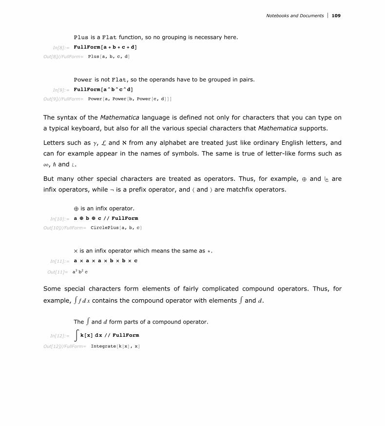
Plus is a Flat function, so no grouping is necessary here.

In[8]:= FullForm@a + b + c + dD

Out[8]//FullForm= Plus@a, b, c, dD

Power is not Flat, so the operands have to be grouped in pairs.

In[9]:= FullForm@a^b^c^dD

Out[9]//FullForm= Power@a, Power@b, Power@c, dDDD

The syntax of the Mathematica language is defined not only for characters that you can type on

a typical keyboard, but also for all the various special characters that Mathematica supports.

Letters such as g, and ¡ from any alphabet are treated just like ordinary English letters, and

can for example appear in the names of symbols. The same is true of letter-like forms such as

¶, — and —.

But many other special characters are treated as operators. Thus, for example, ⊕ and ù are

infix operators, while Ÿ is a prefix operator, and X and \ are matchfix operators.

⊕ is an infix operator.

In[10]:= a ⊕ b ⊕ c êê FullForm

Out[10]//FullForm= CirclePlus@a, b, cD

µ is an infix operator which means the same as *.

In[11]:= a µ a µ a µ b µ b µ c

Out[11]= a3 b2 c

Some special characters form elements of fairly complicated compound operators. Thus, for

example, Ÿ f „ x contains the compound operator with elements Ÿ and „.

The Ÿ and „ form parts of a compound operator.

In[12]:= ‡ k@xD „x êê FullForm

Out[12]//FullForm= Integrate@k@xD, xD


No parentheses are needed here: the “inner precedence” of Ÿ … „ is lower than Times.

In[13]:= ‡ a@xD b@xD „x + c@xD

Out[13]= c@xD + ‡ a@xD b@xD „x

Parentheses are needed here, however.

In[14]:= ‡ Ha@xD + b@xDL „x + c@xD

Out[14]= c@xD + ‡ Ha@xD + b@xDL „x

Input to Mathematica can be given not only in the form of one-dimensional strings, but also in

the form of two-dimensional boxes. The syntax of the Mathematica language covers not only

one-dimensional constructs but also two-dimensional ones.

This superscript is interpreted as a power.

In[15]:= xa+b

Out[15]= xa+b

∂x f is a two-dimensional compound operator.

In[16]:= ∂xxn

Out[16]= n x-1+n

⁄ is part of a more complicated two-dimensional compound operator.

In[17]:= ‚n=1

¶ 1

ns

Out[17]= Zeta@sD

The ⁄ operator has higher precedence than +.

In[18]:= ‚n=1

¶ 1

ns+ n

Out[18]= n + Zeta@sD


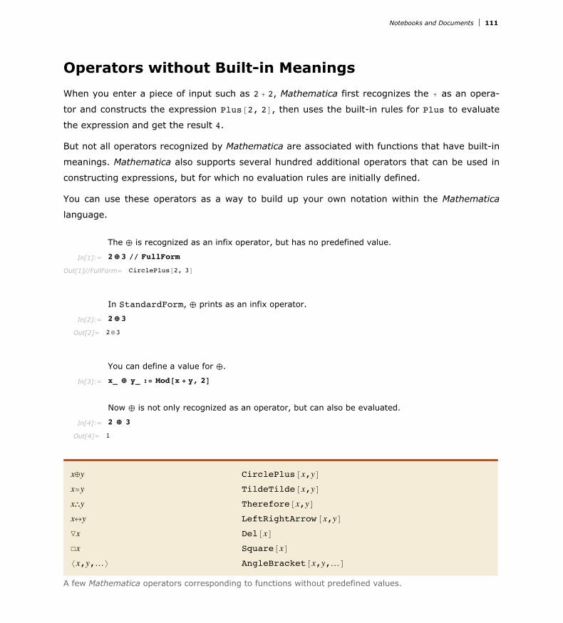
Operators without Built-in Meanings

When you enter a piece of input such as 2 + 2, Mathematica first recognizes the + as an opera-

tor and constructs the expression Plus@2, 2D, then uses the built-in rules for Plus to evaluate

the expression and get the result 4.

But not all operators recognized by Mathematica are associated with functions that have built-in

meanings. Mathematica also supports several hundred additional operators that can be used in

constructing expressions, but for which no evaluation rules are initially defined.

You can use these operators as a way to build up your own notation within the Mathematica

language.

The ⊕ is recognized as an infix operator, but has no predefined value.

In[1]:= 2 ⊕ 3 êê FullForm

Out[1]//FullForm= CirclePlus@2, 3D

In StandardForm, ⊕ prints as an infix operator.

In[2]:= 2 ⊕ 3

Out[2]= 2⊕3

You can define a value for ⊕.

In[3]:= x_ ⊕ y_ := Mod@x + y, 2D

Now ⊕ is not only recognized as an operator, but can also be evaluated.

In[4]:= 2 ⊕ 3

Out[4]= 1

x⊕y CirclePlus@x,yD

xºy TildeTilde@x,yD

x\y Therefore@x,yD

x¨y LeftRightArrow@x,yD

“x Del@xD

Ñx Square@xD

Xx,y,…\ AngleBracket@x,y,…D

A few Mathematica operators corresponding to functions without predefined values.

Mathematica follows the general convention that the function associated with a particular opera-

tor should have the same name as the special character that represents that operator.


Mathematica follows the general convention that the function associated with a particular opera-

tor should have the same name as the special character that represents that operator.

î[Congruent] is displayed as ª.

In[5]:= x ª y

Out[5]= x ª y

It corresponds to the function Congruent.

In[6]:= FullForm@%D

Out[6]//FullForm= Congruent@x, yD

x \@nameD y name[x, y]

î@nameD x name[x]

î@Left nameD x,y,… î@Right nameD name[x, y, …]

The conventional correspondence in Mathematica between operator names and function names.

You should realize that even though the functions CirclePlus and CircleTimes do not have

built-in evaluation rules, the operators ⊕ and ⊗ do have built-in precedences. "Operator Input

Forms" lists all the operators recognized by Mathematica, in order of their precedence.

The operators ⊗ and ⊕ have definite precedences~with ⊗ higher than ⊕.

In[7]:= x ⊗ y ⊕ z êê FullForm

Out[7]//FullForm= Mod@Plus@z, CircleTimes@x, yDD, 2D


xy Subscript@x,yD

x+ SubPlus@xD

x- SubMinus@xD

x* SubStar@xD

x+ SuperPlus@xD

x- SuperMinus@xD

x* SuperStar@xD

x† SuperDagger@xD

xy

Overscript@x,yD

xy

Underscript@x,yD

x OverBar@xD

x” OverVector@xD

xè OverTilde@xD

x` OverHat@xD

x° OverDot@xD

x UnderBar@xD

Some two-dimensional forms without built-in meanings.

Subscripts have no built-in meaning in Mathematica.

In[8]:= x2 + y2 êê InputForm

Out[8]//InputForm= Subscript[x, 2] + Subscript[y, 2]

Most superscripts are however interpreted as powers by default.

In[9]:= x2 + y2 êê InputFormOut[9]//InputForm= x^2 + y^2

A few special superscripts are not interpreted as powers.

In[10]:= x† + y+ êê InputFormOut[10]//InputForm= SuperDagger[x] + SuperPlus[y]

Bar and hat are interpreted as OverBar and OverHat.

In[11]:= x + y` êê InputFormOut[11]//InputForm= OverBar[x] + OverHat[y]

Defining Output Formats


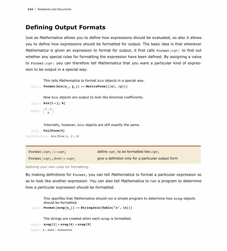
Defining Output Formats

Just as Mathematica allows you to define how expressions should be evaluated, so also it allows

you to define how expressions should be formatted for output. The basic idea is that whenever

Mathematica is given an expression to format for output, it first calls Format@exprD to find out

whether any special rules for formatting the expression have been defined. By assigning a value

to Format@exprD you can therefore tell Mathematica that you want a particular kind of expres-

sion to be output in a special way.

This tells Mathematica to format bin objects in a special way.

In[1]:= Format@bin@x_, y_DD := MatrixForm@88x<, 8y<<D

Now bin objects are output to look like binomial coefficients.

In[2]:= bin@i + j, kD

Out[2]=i + jk

Internally, however, bin objects are still exactly the same.

In[3]:= FullForm@%D

Out[3]//FullForm= bin@Plus@i, jD, kD

Format@expr1D:=expr2 define expr1 to be formatted like expr2Format@expr1, formD:=expr2 give a definition only for a particular output form

Defining your own rules for formatting.

By making definitions for Format, you can tell Mathematica to format a particular expression so

as to look like another expression. You can also tell Mathematica to run a program to determine

how a particular expression should be formatted.

This specifies that Mathematica should run a simple program to determine how xrep objects should be formatted.

In[4]:= Format@xrep@n_DD := StringJoin@Table@"x", 8n<DD

The strings are created when each xrep is formatted.

In[5]:= xrep@1D + xrep@4D + xrep@9D

Out[5]= x + xxxx + xxxxxxxxx

Internally however the expression still contains xrep objects.


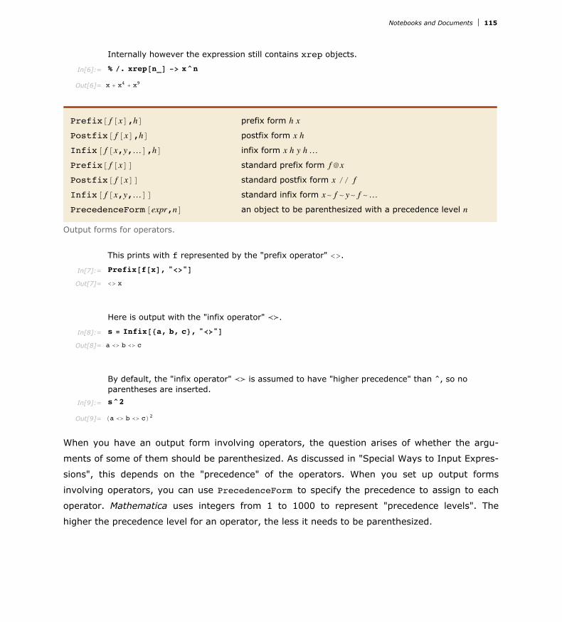
Internally however the expression still contains xrep objects.

In[6]:= % ê. xrep@n_D -> x^n

Out[6]= x + x4 + x9

Prefix@ f@xD,hD prefix form h x

Postfix@ f@xD,hD postfix form x h

Infix@ f@x,y,…D,hD infix form x h y h…Prefix@ f@xDD standard prefix form f üx

Postfix@ f@xDD standard postfix form x êê f

Infix@ f@x,y,…DD standard infix form x~ f ~y~ f ~…PrecedenceForm@expr,nD an object to be parenthesized with a precedence level n

Output forms for operators.

This prints with f represented by the "prefix operator" <>.

In[7]:= Prefix@f@xD, "<>"D

Out[7]= <> x

Here is output with the "infix operator" Äê.

In[8]:= s = Infix@8a, b, c<, "Äê"D

Out[8]= a Äê b Äê c

By default, the "infix operator" Äê is assumed to have "higher precedence" than ^, so no parentheses are inserted.

In[9]:= s^2

Out[9]= Ha Äê b Äê cL2

When you have an output form involving operators, the question arises of whether the argu-

ments of some of them should be parenthesized. As discussed in "Special Ways to Input Expres-

sions", this depends on the "precedence" of the operators. When you set up output forms

involving operators, you can use PrecedenceForm to specify the precedence to assign to each

operator. Mathematica uses integers from 1 to 1000 to represent "precedence levels". The

higher the precedence level for an operator, the less it needs to be parenthesized.


Here Äê is treated as an operator with precedence 100. This precedence turns out to be low enough that parentheses are inserted.

In[10]:= PrecedenceForm@s, 100D^2

Out[10]= Ha Äê b Äê cL2

When you make an assignment for Format@exprD, you are defining the output format for expr in

all standard types of Mathematica output. By making definitions for Format@expr, formD, you can

specify formats to be used in specific output forms.

This specifies the TeXForm for the symbol x.

In[11]:= Format@x, TeXFormD := "8\\bf x<"

The output format for x that you specified is now used whenever the TeX form is needed.

In[12]:= TeXForm@1 + x^2D

Out[12]//TeXForm= x^2+1

Low-Level Input and Output Rules

MakeBoxes@expr, formD construct boxes to represent expr in the specified form

MakeExpression@boxes, formD construct an expression corresponding to boxes

Low-level functions for converting between expressions and boxes.

MakeBoxes generates boxes without evaluating its input.

In[1]:= MakeBoxes@2 + 2, StandardFormD

Out[1]= RowBox@82, +, 2<D

MakeExpression interprets boxes but uses HoldComplete to prevent the resulting expression from being evaluated.

In[2]:= MakeExpression@%, StandardFormD

Out[2]= HoldComplete@2 + 2D

Built into Mathematica are a large number of rules for generating output and interpreting input.

Particularly in StandardForm, these rules are carefully set up to be consistent, and to allow

input and output to be used interchangeably.

It is fairly rare that you will need to modify these rules. The main reason is that Mathematica

already has built-in rules for the input and output of many operators to which it does not itself

assign specific meanings.


It is fairly rare that you will need to modify these rules. The main reason is that Mathematica

already has built-in rules for the input and output of many operators to which it does not itself

assign specific meanings.

Thus, if you want to add, for example, a generalized form of addition, you can usually just use

an operator like ⊕ for which Mathematica already has built-in input and output rules.

This outputs using the ⊕ operator.

In[3]:= CirclePlus@u, v, wD

Out[3]= u⊕v⊕w

Mathematica understands ⊕ on input.

In[4]:= u ⊕ v ⊕ w êê FullForm

Out[4]//FullForm= CirclePlus@u, v, wD

In dealing with output, you can make definitions for Format@exprD to change the way that a

particular expression will be formatted. You should realize, however, that as soon as you do

this, there is no guarantee that the output form of your expression will be interpreted correctly

if it is given as Mathematica input.

If you want to, Mathematica allows you to redefine the basic rules that it uses for the input and

output of all expressions. You can do this by making definitions for MakeBoxes and

MakeExpression. You should realize, however, that unless you make such definitions with great

care, you are likely to end up with inconsistent results.

This defines how gplus objects should be output in StandardForm.

In[5]:= gplus ê: MakeBoxes@gplus@x_, y_, n_D, StandardFormD :=RowBox@8MakeBoxes@x, StandardFormD,

SubscriptBox@"⊕", MakeBoxes@n, StandardFormDD, MakeBoxes@y, StandardFormD<D

gplus is now output using a subscripted ⊕.

In[6]:= gplus@a, b, m + nD

Out[6]= a⊕m+n b

Mathematica cannot however interpret this as input.

In[7]:= a ⊕m+n b

Syntax::sntxi : Incomplete expression; more input is needed.


This tells Mathematica to interpret a subscripted ⊕ as a specific piece of FullForm input.

In[8]:= MakeExpression@RowBox@8x_, SubscriptBox@"⊕", n_D, y_<D, StandardFormD :=MakeExpression@RowBox@8"gplus", "@", x, ",", y, ",", n, "D"<D, StandardFormD

Now the subscripted ⊕ is interpreted as a gplus.

In[9]:= a ⊕m+n b êê FullForm

Out[9]//FullForm= gplus@a, b, Plus@m, nDD

When you give definitions for MakeBoxes, you can think of this as essentially a lower-level

version of giving definitions for Format. An important difference is that MakeBoxes does not

evaluate its argument, so you can define rules for formatting expressions without being con-

cerned about how these expressions would evaluate.

In addition, while Format is automatically called again on any results obtained by applying it,

the same is not true of MakeBoxes. This means that in giving definitions for MakeBoxes you

explicitly have to call MakeBoxes again on any subexpressions that still need to be formatted.

† Break input into tokens.

† Strip spacing characters.

† Construct boxes using built-in operator precedences.

† Strip StyleBox and other boxes not intended for interpretation.

† Apply rules defined for MakeExpression.

Operations done on Mathematica input.

Generating Unstructured Output

The functions described in "Textual Input and Output Overview" determine how expressions

should be formatted when they are printed, but they do not actually cause anything to be

printed.

In the most common way of using Mathematica you never in fact explicitly have to issue a

command to generate output. Usually, Mathematica automatically prints out the final result that

it gets from processing input you gave. Sometimes, however, you may want to get Mathemat-

ica to print out expressions at intermediate stages in its operation. You can do this using the

function Print.


Print@expr1,expr2,…D print the expri, with no spaces in between, but with a

newline (line feed) at the end

Printing expressions.

Print prints its arguments, with no spaces in between, but with a newline (line feed) at the end.

In[1]:= Print@a, bD; Print@cD

ab

c

This prints a table of the first five integers and their squares.

In[2]:= Do@Print@i, " ", i^2D, 8i, 5<D

1 1

2 4

3 9

4 16

5 25

Print simply takes the arguments you give, and prints them out one after the other, with no

spaces in between. In many cases, you will need to print output in a more complicated format.

You can do this by giving an output form as an argument to Print.

This prints the matrix in the form of a table.

In[3]:= Print@Grid@881, 2<, 83, 4<<DD

1 23 4

Here the output format is specified using StringForm.

In[4]:= Print@StringForm@"x = ``, y = ``", a^2, b^2DD

x = a2, y = b2


Print also allows mixing of text and graphics.

In[5]:= Print@"A sine wave:", Plot@Sin@xD, 8x, 0, 2 p<DD

A sine wave:1 2 3 4 5 6

-1.0

-0.5

0.5

1.0

The output generated by Print is usually given in the standard Mathematica output format.

You can however explicitly specify that some other output format should be used.

This prints output in Mathematica input form.

In[6]:= Print@InputForm@a^2 + b^2DD

a^2 + b^2

You should realize that Print is only one of several mechanisms available in Mathematica for

generating output. Another is the function Message described in "Messages", used for generat-

ing named messages. There are also a variety of lower-level functions described in "Streams

and Low-Level Input and Output" which allow you to produce output in various formats both as

part of an interactive session, and for files and external programs.

Another command which works exactly like Print, but only shows the printed output until the

final evaluation is finished, is PrintTemporary.


Formatted Output

Ever since Version 3 of Mathematica, there has been rich support for arbitrary mathematical

typesetting and layout. Underlying all that power was a so-called box language, which allowed

notebooks themselves to be Mathematica expressions. This approach turned out to be very

powerful, and has formed the basis of many unique features in Mathematica. However, despite

the power of the box language, in practice it was awkward enough for users to access directly

that few did.

Starting in Version 6, there is a higher-level interface to this box language which takes much of

the pain out of using boxes directly, while still exposing all the same typesetting and layout

power. Functions in this new layer are often referred to as box generators, but there is no need

for you to be aware of the box language to use them effectively. In this tutorial, we will take a

look at box generators that are relevant for displaying a wide variety of expressions, and we

will show some ways in which they can be used to generate beautifully formatted output that

goes beyond simple mathematical typesetting.

Styling Output

The Mathematica front end supports all the usual style mechanisms available in word proces-

sors, for example including menus for changing font characteristics. However, it used to be very

difficult to access those styling mechanisms automatically in generated output. Output contin-

ued to be almost universally plain 12 pt. Courier (or Times for those people using

TraditionalForm). To address this, the function Style was created. Whenever you evaluate a

Style expression, its output will be displayed with the given style attributes active.

You can wrap Style around any sort of expression. Here is an example that displays prime and

composite numbers using different font weights and colors via Style.

In[1]:= Table@If@PrimeQ@iD, Style@i, BoldD, Style@i, GrayDD, 8i, 1, 100<D

Out[1]= 81, 2, 3, 4, 5, 6, 7, 8, 9, 10, 11, 12, 13, 14, 15, 16, 17, 18, 19, 20, 21, 22, 23, 24, 25, 26, 27, 28,29, 30, 31, 32, 33, 34, 35, 36, 37, 38, 39, 40, 41, 42, 43, 44, 45, 46, 47, 48, 49, 50, 51, 52,53, 54, 55, 56, 57, 58, 59, 60, 61, 62, 63, 64, 65, 66, 67, 68, 69, 70, 71, 72, 73, 74, 75, 76,77, 78, 79, 80, 81, 82, 83, 84, 85, 86, 87, 88, 89, 90, 91, 92, 93, 94, 95, 96, 97, 98, 99, 100<

There are hundreds of formatting options that you could apply with Style~see the documenta-

tion for Style for a more complete listing~but there are a handful that are by far the most

common, listed here.


Menu Style@D option Style@D directive

Format Size 14 FontSize -> 14 14

Format Text Color Gray FontColor -> Gray Gray

Format Face Bold FontWeight -> Bold Bold

Format Face Italic FontSlant -> Italic Italic

Format Background Color Yellow Background -> Yellow

Format Font FontFamily -> "Times"

Format Style Subsection "Subsection"

Note that Style can be arbitrarily nested, with the innermost one taking precedence if there is

a conflict. Here we wrap Style around the entire list to apply a new font to all elements of the

list.

In[2]:= Style@%, FontFamily Ø "Helvetica"D

Out[2]= 81, 2, 3, 4, 5, 6, 7, 8, 9, 10, 11, 12, 13, 14, 15, 16, 17, 18, 19, 20, 21, 22, 23, 24, 25, 26, 27, 28, 29, 30, 31, 32, 33, 34, 35, 36, 37,38, 39, 40, 41, 42, 43, 44, 45, 46, 47, 48, 49, 50, 51, 52, 53, 54, 55, 56, 57, 58, 59, 60, 61, 62, 63, 64, 65, 66, 67, 68, 69,70, 71, 72, 73, 74, 75, 76, 77, 78, 79, 80, 81, 82, 83, 84, 85, 86, 87, 88, 89, 90, 91, 92, 93, 94, 95, 96, 97, 98, 99, 100<

Another common thing to want is to have a portion of the output styled like text. It can look

quite strange to have text appear in a font which is intended for use by code. For that purpose,

we have a function Text which ensures that its argument will always be rendered in a text font.

(Those of you familiar with Mathematica graphics will recognize the Text function as a graphics

primitive, but that use does not conflict with this use outside of graphics.)

In[3]:= Text@%%D

Out[3]= 81, 2, 3, 4, 5, 6, 7, 8, 9, 10, 11, 12, 13, 14, 15, 16, 17, 18, 19, 20, 21, 22, 23, 24, 25, 26, 27, 28, 29, 30, 31, 32, 33, 34,35, 36, 37, 38, 39, 40, 41, 42, 43, 44, 45, 46, 47, 48, 49, 50, 51, 52, 53, 54, 55, 56, 57, 58, 59, 60, 61, 62, 63, 64, 65, 66, 67,68, 69, 70, 71, 72, 73, 74, 75, 76, 77, 78, 79, 80, 81, 82, 83, 84, 85, 86, 87, 88, 89, 90, 91, 92, 93, 94, 95, 96, 97, 98, 99, 100<

Style can be used to set up a region on the screen where any option is active, not just options

related to fonts. Later in this tutorial, we will see how Style can even affect the display charac-

teristics of other formatting constructs, like Grid or Tooltip.

Grid Layout

Using two-dimensional layout structures can be just as useful as applying style directives to

those structures. In Mathematica, the primary function for such layout is Grid. Grid has very

flexible layout features, including the ability to arbitrarily adjust things like alignment, frame

elements, and spanning elements. (Other tutorials go into Grid's features in greater detail, but

we will cover the highlights here.)

Look again at the Style example which displays prime and composite numbers differently.


Look again at the Style example which displays prime and composite numbers differently.

In[11]:= ptable = Table@If@PrimeQ@iD, Style@i, BoldD, Style@i, GrayDD, 8i, 1, 100<D;

To put this into a Grid, we first use Partition to turn this 100-element list into a 10×10 array.

Although you can give Grid a ragged array (a list whose elements are lists of different lengths),

in this case we give Grid a regular array, and the resulting display is a nicely formatted layout.

Grid@Partition@ptable, 10DD

1 2 3 4 5 6 7 8 9 1011 12 13 14 15 16 17 18 19 2021 22 23 24 25 26 27 28 29 3031 32 33 34 35 36 37 38 39 4041 42 43 44 45 46 47 48 49 5051 52 53 54 55 56 57 58 59 6061 62 63 64 65 66 67 68 69 7071 72 73 74 75 76 77 78 79 8081 82 83 84 85 86 87 88 89 9091 92 93 94 95 96 97 98 99 100

Notice that the columns are aligned on center, and there are no frame lines. It is an easy mat-

ter to change either of these using Grid's options.

Grid@Partition@ptable, 10D, Alignment Ø Right,Frame Ø True, Background Ø LightBlueD

1 2 3 4 5 6 7 8 9 1011 12 13 14 15 16 17 18 19 2021 22 23 24 25 26 27 28 29 3031 32 33 34 35 36 37 38 39 4041 42 43 44 45 46 47 48 49 5051 52 53 54 55 56 57 58 59 6061 62 63 64 65 66 67 68 69 7071 72 73 74 75 76 77 78 79 8081 82 83 84 85 86 87 88 89 9091 92 93 94 95 96 97 98 99 100

A complete description of all Grid's options and their syntax is beyond the scope of this docu-

ment, but it is possible to do some remarkable things with them. See the complete Grid docu-

mentation for complete details.

There are a few convenience constructs related to Grid. One is Column, which takes a flat list of

elements and arranges them vertically. This would be slightly awkward to do with Grid. Here is

a simple example, viewing the options of column in, well, a column.


Column@Options@ColumnDD

Alignment Ø 8Left, Baseline<Background Ø NoneBaselinePosition Ø AutomaticBaseStyle Ø 8<

ColumnAlignments Ø LeftDefaultBaseStyle Ø GridDefaultElement Ø Ñ

Dividers Ø NoneFrame Ø NoneFrameStyle Ø AutomaticItemSize Ø AutomaticItemStyle Ø NoneSpacings Ø 80.8, 1.<

What about laying out a list of things horizontally? In that case, the main question you need to

ask is whether you want the resulting display to line wrap like a line of math or text would, or

whether you want the elements to remain on a single line. In the latter case, you would use

Grid applied to a 1×n array.

In[5]:= Grid@8Range@15D!<D

Out[5]=1 2 6 24 120 720 5040 40320 362880 3628800 39916800 4790016Ö

006227020Ö800

8717829Ö1200

1307674Ö368000

But notice in this example, that the overall grid shrinks so that it fits in the available window

width. As a result, there are elements of the grid which themselves wrap onto multiple lines.

This is due to the default ItemSize option of Grid. If you want to allow the elements of a grid

to be as wide as they would naturally be, set ItemSize to Full.

In[7]:= Grid@8Range@15D!<, ItemSize Ø FullD

Out[7]= 1 2 6 24 120 720 5040 40320 362880 3628800 39916800 479001600 6227020800 87178291200 1307674368000

Of course, now the whole grid is too wide to fit on one line (unless you make this window very

wide), and so there are elements in the grid which you cannot see. That brings us to the other

horizontal layout function: Row.

Given a list of elements, Row will allow the overall result to word wrap in the natural way, just

like a line of text or math would. This type of layout will be familiar to those of you who might

have used the old (and now obsolete) SequenceForm function.

Row@Range@15D!D

12624120720504040 320362 880362880039 916800479 001600622702080087 1782912001307674368000

As you can see, Row does not leave space between elements by default. But if you give a sec-

ond argument, that expression is inserted between elements. Here we use a comma, but any

expression can be used.


As you can see, Row does not leave space between elements by default. But if you give a sec-

ond argument, that expression is inserted between elements. Here we use a comma, but any

expression can be used.

Row@Range@15D!, ","D

1, 2, 6, 24, 120, 720, 5040, 40320, 362880, 3628800, 39916800,479001600, 6227020800, 87178291200, 1307674368000

If you resize the notebook window, you will see that Grid with ItemSize -> Automatic contin-

ues to behave differently than Row, and each is useful in different circumstances.

Using Output as Input

This is a good time to point out that Style, Grid, and all other box generators are persistent in

output. If you were to take a piece of output that had some formatting created by Style or

Grid and reuse that as input, the literal Style or Grid expressions would appear in the input

expression. Those of you familiar with the old uses of StyleBox and even functions like

MatrixForm will find this a change.

Consider taking the output of this Grid command, which has lots of embedded styles, and

using it in some input expression.

In[17]:= Grid@Partition@Take@ptable, 16D, 4D,Alignment Ø Right, Frame Ø True, Background Ø LightBlueD

Out[17]=

In[18]:=

1 2 3 45 6 7 89 10 11 12

13 14 15 16

+ 5

3

êê Expand

Out[18]= 125 + 75

1 2 3 45 6 7 89 10 11 1213 14 15 16

+ 15

1 2 3 45 6 7 89 10 11 1213 14 15 16

2

+

1 2 3 45 6 7 89 10 11 1213 14 15 16

3

Notice that the grid is still a grid, it is still blue, and the elements are still bold or gray as

before. Also notice that having literal Grid and Style in the expression interferes with what

would have otherwise been adding a scalar to a matrix, and raising the result to a power. This


1 2 3 45 6 7 89 10 11 1213 14 15 16

Notice that the grid is still a grid, it is still blue, and the elements are still bold or gray as

before. Also notice that having literal Grid and Style

distinction is very important, since you almost always want these composite structures to resist

being interpreted automatically in some way. However, if you ever do want to get rid of these

wrappers and get at your data, that is easy enough to do.

In[19]:= % êê. 8Grid@a_, ___D ß a, Style@a_, ___D ß a<

Out[19]= 88216, 343, 512, 729<, 81000, 1331, 1728, 2197<, 82744, 3375, 4096, 4913<, 85832, 6859, 8000, 9261<<

Special Grid Entries

To allow more flexible two-dimensional layout, Grid accepts a few special symbols like

SpanFromLeft as entries. The entry SpanFromLeft indicates that the grid entry immediately to

the left should take up its own space and also the space of the spanning character. There are

also SpanFromAbove and SpanFromBoth. See "Grids, Rows, and Columns" for detailed

information.

Grid@881, 2, 3, 4, 5<,86, 7, SpanFromLeft, SpanFromLeft, 10<,811, SpanFromAbove, SpanFromBoth, SpanFromBoth, 15<,816, 17, 18, 19, 20<<, Frame Ø AllD

1 2 3 4 56 7 1011 1516 17 18 19 20

This approach can be used to create complicated spanning setups. Typing something like the

following as an input would take a long time. Luckily you can create this table interactively by

using Make Spanning and Split Spanning in the Insert Table/Matrix submenu. If you

want to see what would be involved in typing this, evaluate the cell, which will show how it

should be typed as input.

In[18]:=

1 2 3 4 5 6 7 8 9 1011 12 13 15 1621 22 2531 32 33 34 35

4151 52 53 54 5561 62 6371 72 76 7781 82 8691 92 96

êê InputForm

We have already seen how to apply things like alignment and background to a grid as a whole,

or to individual columns or rows. What we have not seen though is how to override that for an

individual element. Say you want your whole grid to have the same background, except for a

few special elements. A convenient way to do that is to wrap each such element in Item, and

then specify options to Item which override the corresponding option in Grid.


We have already seen how to apply things like alignment and background to a grid as a whole,

or to individual columns or rows. What we have not seen though is how to override that for an

individual element. Say you want your whole grid to have the same background, except for a

few special elements. A convenient way to do that is to wrap each such element in Item, and

then specify options to Item which override the corresponding option in Grid.

Grid@Partition@Table@If@PrimeQ@iD, Item@i, Background Ø LightYellowD, iD,8i, 1, 100<D, 10D, Background Ø LightBlueD

1 2 3 4 5 6 7 8 9 1011 12 13 14 15 16 17 18 19 2021 22 23 24 25 26 27 28 29 3031 32 33 34 35 36 37 38 39 4041 42 43 44 45 46 47 48 49 5051 52 53 54 55 56 57 58 59 6061 62 63 64 65 66 67 68 69 7071 72 73 74 75 76 77 78 79 8081 82 83 84 85 86 87 88 89 9091 92 93 94 95 96 97 98 99 100

You could override this option with Style too, but the purpose of Item is to override it in a way

that knows about the two-dimensional layout of Grid. Notice in the preceeding output that

whenever two of the yellow cells are next to each other, there is no blue space between them.

That would be impossible to do with constructs other than Item.

The same thing goes for all Item's options, not just Background. Consider the Frame option. If

you want no frame elements except around certain specified elements, you might think that

you have to wrap them in their own Grid with the Frame -> True setting. (We will learn a much

easier way to add a frame around an arbitrary expression in the next section.)

Grid@Partition@Table@If@PrimeQ@iD, Grid@88i<<, Frame Ø TrueD, iD, 8i, 1, 100<D, 10DD

1 2 3 4 5 6 7 8 9 10

11 12 13 14 15 16 17 18 19 20

21 22 23 24 25 26 27 28 29 30

31 32 33 34 35 36 37 38 39 40

41 42 43 44 45 46 47 48 49 50

51 52 53 54 55 56 57 58 59 60

61 62 63 64 65 66 67 68 69 70

71 72 73 74 75 76 77 78 79 80

81 82 83 84 85 86 87 88 89 90

91 92 93 94 95 96 97 98 99 100

But notice that adjacent framed elements do not share their boundaries. Compare that with

using Item, below, which has enough information to not draw more frame elements than are

necessary. Notice now the frames of 2 and 11 meet at a single point, and how the frames of 2

and 3 share a single-pixel line, which in turn is perfectly aligned with the left frame of 13 and

23. That is the power of Item.


But notice that adjacent framed elements do not share their boundaries. Compare that with

using Item, below, which has enough information to not draw more frame elements than are

necessary. Notice now the frames of 2 and 11 meet at a single point, and how the frames of 2

and 3 share a single-pixel line, which in turn is perfectly aligned with the left frame of 13 and

23. That is the power of Item.

Grid@Partition@Table@If@PrimeQ@iD, Item@i, Frame Ø TrueD, iD, 8i, 1, 100<D, 10DD

1 2 3 4 5 6 7 8 9 1011 12 13 14 15 16 17 18 19 2021 22 23 24 25 26 27 28 29 3031 32 33 34 35 36 37 38 39 4041 42 43 44 45 46 47 48 49 5051 52 53 54 55 56 57 58 59 6061 62 63 64 65 66 67 68 69 7071 72 73 74 75 76 77 78 79 8081 82 83 84 85 86 87 88 89 9091 92 93 94 95 96 97 98 99 100

Frames and Labels

Adding a frame or a label to an expression can be done with Grid, but conceptually these are

much simpler operations than general two-dimensional layout, and so there are correspondingly

simpler ways to get them. For instance, Framed is a simple function for drawing a frame around

an arbitrary expression. This can be useful to draw attention to parts of an expression, for

instance.

Table@If@PrimeQ@iD, Framed@i, Background Ø LightYellowD, iD, 8i, 1, 100<D

:1, 2 , 3 , 4, 5 , 6, 7 , 8, 9, 10, 11 , 12, 13 , 14, 15, 16, 17 , 18, 19 , 20,

21, 22, 23 , 24, 25, 26, 27, 28, 29 , 30, 31 , 32, 33, 34, 35, 36, 37 , 38, 39, 40,

41 , 42, 43 , 44, 45, 46, 47 , 48, 49, 50, 51, 52, 53 , 54, 55, 56, 57, 58, 59 , 60,

61 , 62, 63, 64, 65, 66, 67 , 68, 69, 70, 71 , 72, 73 , 74, 75, 76, 77, 78, 79 , 80,

81, 82, 83 , 84, 85, 86, 87, 88, 89 , 90, 91, 92, 93, 94, 95, 96, 97 , 98, 99, 100>

Labeled is another such function, which allows labels to be placed at arbitrary locations around

a given expression. Here we add a legend to the Grid example from the last section. (Spacer is

just a function that is designed to leave empty space.)


In[19]:= Labeled@Grid@Partition@ptable, 10D, Alignment Ø Right, Frame Ø TrueD,Text@Row@8Style@"• Prime", BoldD, Style@"• Composite", GrayD<, Spacer@15DDDD

Out[19]=

Panel is yet another framing construct, which uses the underlying operating system's panel

frame. This is different from Frame, as different operating systems might use a drop shadow,

rounded corners, or fancier graphic design elements for a panel frame.

In[20]:= Panel@%D

Out[20]=

Note that Panel has its own concept of font family and size as well, so the contents of Grid

change font family and size, and the Text changes font size. (Text has its own opinion about

font family though, and so it remains in Mathematica's text font.) We will talk about this in

some detail below in the section on the BaseStyle option.

Finally, we should point out that Panel itself has an optional second argument to specify one or

more labels, which are automatically positioned outside the panel, and an optional third argu-

ment to give details of that position. See the documentation for Panel for more detail.

In[37]:= Panel@ptable, "Primes and Composites"D

Out[37]=


1 2 3 4 5 6 7 8 9 1011 12 13 14 15 16 17 18 19 2021 22 23 24 25 26 27 28 29 3031 32 33 34 35 36 37 38 39 4041 42 43 44 45 46 47 48 49 5051 52 53 54 55 56 57 58 59 6061 62 63 64 65 66 67 68 69 7071 72 73 74 75 76 77 78 79 8081 82 83 84 85 86 87 88 89 9091 92 93 94 95 96 97 98 99 100

• Prime • Composite

1 2 3 4 5 6 7 8 9 1011 12 13 14 15 16 17 18 19 2021 22 23 24 25 26 27 28 29 3031 32 33 34 35 36 37 38 39 4041 42 43 44 45 46 47 48 49 5051 52 53 54 55 56 57 58 59 6061 62 63 64 65 66 67 68 69 7071 72 73 74 75 76 77 78 79 8081 82 83 84 85 86 87 88 89 9091 92 93 94 95 96 97 98 99 100

• Prime • Composite

Primes and Composites

81, 2 , 3 , 4, 5 , 6, 7 , 8, 9, 10 , 11 , 12 , 13 , 14 , 15 , 16 , 17 , 18 , 19 , 20 , 21 , 22 , 23 , 24 , 25 , 26 , 27 , 28 , 29 , 30 , 31 , 32 , 33 , 34 , 35 , 36 , 37 ,38 , 39 , 40 , 41 , 42 , 43 , 44 , 45 , 46 , 47 , 48 , 49 , 50 , 51 , 52 , 53 , 54 , 55 , 56 , 57 , 58 , 59 , 60 , 61 , 62 , 63 , 64 , 65 , 66 , 67 , 68 , 69 ,70 , 71 , 72 , 73 , 74 , 75 , 76 , 77 , 78 , 79 , 80 , 81 , 82 , 83 , 84 , 85 , 86 , 87 , 88 , 89 , 90 , 91 , 92 , 93 , 94 , 95 , 96 , 97 , 98 , 99 , 100 <

In[38]:= Panel@ptable, 8"Primes and Composites"<, 88Bottom, Right<<D

Out[38]=

Other Annotations

The annotations mentioned so far have a very definite visual component. There are a number of

annotations which are effectively invisible, until the user needs them. Tooltip for example

does not change the display of its first argument, and only when you move the mouse pointer

over that display is the second argument shown, as a tooltip.

Table@Tooltip@i, Divisors@iDD, 8i, 1, 100<D

81, 2, 3, 4, 5, 6, 7, 8, 9, 10, 11, 12, 13, 14, 15, 16, 17, 18, 19, 20, 21, 22, 23, 24, 25, 26, 27, 28,29, 30, 31, 32, 33, 34, 35, 36, 37, 38, 39, 40, 41, 42, 43, 44, 45, 46, 47, 48, 49, 50, 51, 52,53, 54, 55, 56, 57, 58, 59, 60, 61, 62, 63, 64, 65, 66, 67, 68, 69, 70, 71, 72, 73, 74, 75, 76,77, 78, 79, 80, 81, 82, 83, 84, 85, 86, 87, 88, 89, 90, 91, 92, 93, 94, 95, 96, 97, 98, 99, 100<

Mouseover is another such function, but instead of displaying the result in a tooltip, it uses the

same area of the screen that had been used for the display before you moved the mouse

pointer over it. If the two displays are different sizes, then the effect can be jarring, so it is a

good idea to use displays which are closer to the same size, or use the Mouseover ImageSize

option to leave space for the larger of the two displays, regardless of which is being displayed.

Table@Mouseover@i, Framed@Divisors@iD, Background Ø LightYellowDD, 8i, 1, 100<D

81, 2, 3, 4, 5, 6, 7, 8, 9, 10, 11, 12, 13, 14, 15, 16, 17, 18, 19, 20, 21, 22, 23, 24, 25, 26, 27,28, 29, 30, 31, 32, 33, 34, 35, 36, 37, 38, 39, 40, 41, 42, 43, 44, 45, 46, 47, 48, 49, 50, 51, 52,53, 54, 55, 56, 57, 58, 59, 60, 61, 62, 63, 64, 65, 66, 67, 68, 69, 70, 71, 72, 73, 74, 75, 76,77, 78, 79, 80, 81, 82, 83, 84, 85, 86, 87, 88, 89, 90, 91, 92, 93, 94, 95, 96, 97, 98, 99, 100<

Also similar to Tooltip are StatusArea and PopupWindow. StatusArea displays the extra

information in the notebook's status area, typically in the lower-left corner, while PopupWindow

will display extra information in a new window when clicked.

Table@StatusArea@i, Divisors@iDD, 8i, 1, 100<D


1, 2 , 3 , 4, 5 , 6, 7 , 8, 9, 10 , 11 , 12 , 13 , 14 , 15 , 16 , 17 , 18 , 19 , 20 , 21 , 22 , 23 , 24 , 25 , 26 , 27 , 28 , 29 , 30 , 31 , 32 , 33 , 34 , 35 , 36 , 37 ,38 , 39 , 40 , 41 , 42 , 43 , 44 , 45 , 46 , 47 , 48 , 49 , 50 , 51 , 52 , 53 , 54 , 55 , 56 , 57 , 58 , 59 , 60 , 61 , 62 , 63 , 64 , 65 , 66 , 67 , 68 , 69 ,70 , 71 , 72 , 73 , 74 , 75 , 76 , 77 , 78 , 79 , 80 , 81 , 82 , 83 , 84 , 85 , 86 , 87 , 88 , 89 , 90 , 91 , 92 , 93 , 94 , 95 , 96 , 97 , 98 , 99 , 100

Primes and Composites

1,2, 3, 4, 5, 6, 7, 8, 9, 10, 11, 12, 13, 14, 15, 16, 17, 18, 19, 20, 21, 22, 23, 24, 25, 26, 27, 28,29, 30, 31, 32, 33, 34, 35, 36, 37, 38, 39, 40, 41, 42, 43, 44, 45, 46, 47, 48, 49, 50, 51, 52,53, 54, 55, 56, 57, 58, 59, 60, 61, 62, 63, 64, 65, 66, 67, 68, 69, 70, 71, 72, 73, 74, 75, 76,77, 78, 79, 80, 81, 82, 83, 84, 85, 86, 87, 88, 89, 90, 91, 92, 93, 94, 95, 96, 97, 98, 99, 100

Table@PopupWindow@i, Divisors@iDD, 8i, 1, 100<D

Finally, you can specify an arbitrary location for an annotation by using the pair Annotation

and MouseAnnotation.

Table@Annotation@i, Divisors@iD, "Mouse"D, 8i, 1, 100<DDynamic@MouseAnnotation@DD

Null

When using annotations that are triggered merely by moving the mouse pointer over a region

of the screen, it is important to keep the user in mind. Moving the mouse is not something that

should trigger a long evaluation or a lot of visual clutter. But used sparingly, annotations can be

quite helpful to users.

Finally, note that all these annotations work perfectly well in graphics too. So you can provide

tooltips or mouseovers to aid users in understanding a complicated graphic you have created.

In fact, even visualization functions like ListPlot or DensityPlot support Tooltip. See the

documentation for details.

In[2]:= Graphics@8LightBlue, EdgeForm@GrayD, Tooltip@CountryData@Ò, "SchematicPolygon"D,Panel@CountryData@Ò, "Flag"D, ÒDD & êü CountryData@D<, ImageSize Ø FullD

Out[2]=


81, 2, 3, 4, 5, 6, 7, 8, 9, 10, 11, 12, 13, 14, 15, 16, 17, 18, 19, 20, 21, 22, 23, 24, 25, 26, 27, 28,29, 30, 31, 32, 33, 34, 35, 36, 37, 38, 39, 40, 41, 42, 43, 44, 45, 46, 47, 48, 49, 50, 51, 52,53, 54, 55, 56, 57, 58, 59, 60, 61, 62, 63, 64, 65, 66, 67, 68, 69, 70, 71, 72, 73, 74, 75, 76,77, 78, 79, 80, 81, 82, 83, 84, 85, 86, 87, 88, 89, 90, 91, 92, 93, 94, 95, 96, 97, 98, 99, 100<

81, 2, 3, 4, 5, 6, 7, 8, 9, 10, 11, 12, 13, 14, 15, 16, 17, 18, 19, 20, 21, 22, 23, 24, 25, 26, 27,28, 29, 30, 31, 32, 33, 34, 35, 36, 37, 38, 39, 40, 41, 42, 43, 44, 45, 46, 47, 48, 49, 50, 51, 52,53, 54, 55, 56, 57, 58, 59, 60, 61, 62, 63, 64, 65, 66, 67, 68, 69, 70, 71, 72, 73, 74, 75, 76,77, 78, 79, 80, 81, 82, 83, 84, 85, 86, 87, 88, 89, 90, 91, 92, 93, 94, 95, 96, 97, 98, 99, 100<

Default Styles

As we saw in the section "Frames and Labels", constructs like Panel actually work much like

Style, in that they set up an environment in which a set of default styles is applied to their

contents. This can be overridden by explicit Style commands, but it can also be overridden for

the Panel itself, through the BaseStyle option. BaseStyle can be set to a style or a list of

style directives, just like you would use in Style. And those directives then become the ambi-

ent default within the scope of that Panel.

As we have already seen, Panel by default uses the dialog font family and size. But that can be

overridden by using this BaseStyle option.

Panel@Range@10DD

81, 2, 3, 4, 5, 6, 7, 8, 9, 10<

In[7]:= Panel@Range@10D, BaseStyle Ø 8"StandardForm"<D

Out[7]= 81, 2, 3, 4, 5, 6, 7, 8, 9, 10<

Actually, almost all of these box generators have a BaseStyle option. For instance, here is a

grid in which the default font color is blue. Notice that the elements that were gray stay gray,

since the inner Style wrapper trumps the outer Grid BaseStyle. (This is one of the principal

characteristics of option inheritance, which is beyond the scope of this document to discuss.)

Grid@Partition@ptable, 10D, BaseStyle Ø 8FontColor Ø Blue<D


1 2 3 4 5 6 7 8 9 10

11 12 13 14 15 16 17 18 19 20

21 22 23 24 25 26 27 28 29 30

31 32 33 34 35 36 37 38 39 40

41 42 43 44 45 46 47 48 49 50

51 52 53 54 55 56 57 58 59 60

61 62 63 64 65 66 67 68 69 70

71 72 73 74 75 76 77 78 79 80

81 82 83 84 85 86 87 88 89 90

91 92 93 94 95 96 97 98 99 100

Default Options

Say you have an expression with multiple occurrences of the same box generator, like a Framed

or a Panel, and you want to change all of them to have the same set of options. It might be

cumbersome to go through and add the same set of options to every occurrence of that func-

tion. Thankfully, there is an easier way.

DefaultOptions is an option to Style which, when set to a list of elements of the form

head -> 8opt -> val, …<. sets up an environment with the given options as the ambient default

for the given box-generating head. Those options will be active throughout the Style wrapper,

but only in any instances of the associated box generator.

So if you had an expression that contained some Framed items, and you wanted them all to be

drawn with the same background and frame style.

Table@If@PrimeQ@iD, Framed@iD, iD, 8i, 1, 100<D

Actually, that input is too short to see the advantage of this syntax. Say you had this same list,

but specified manually.

biglist = 81, Framed@2D, Framed@3D, 4, Framed@5D, 6, Framed@7D, 8, 9, 10,Framed@11D, 12, Framed@13D, 14, 15, 16, Framed@17D, 18, Framed@19D, 20,21, 22, Framed@23D, 24, 25, 26, 27, 28, Framed@29D, 30, Framed@31D, 32, 33,34, 35, 36, Framed@37D, 38, 39, 40, Framed@41D, 42, Framed@43D, 44, 45, 46,Framed@47D, 48, 49, 50, 51, 52, Framed@53D, 54, 55, 56, 57, 58, Framed@59D,60, Framed@61D, 62, 63, 64, 65, 66, Framed@67D, 68, 69, 70, Framed@71D, 72,Framed@73D, 74, 75, 76, 77, 78, Framed@79D, 80, 81, 82, Framed@83D, 84, 85,86, 87, 88, Framed@89D, 90, 91, 92, 93, 94, 95, 96, Framed@97D, 98, 99, 100<

:1, 2 , 3 , 4, 5 , 6, 7 , 8, 9, 10, 11 , 12, 13 , 14, 15, 16, 17 , 18, 19 , 20,

21, 22, 23 , 24, 25, 26, 27, 28, 29 , 30, 31 , 32, 33, 34, 35, 36, 37 , 38, 39, 40,

41 , 42, 43 , 44, 45, 46, 47 , 48, 49, 50, 51, 52, 53 , 54, 55, 56, 57, 58, 59 , 60,

61 , 62, 63, 64, 65, 66, 67 , 68, 69, 70, 71 , 72, 73 , 74, 75, 76, 77, 78, 79 , 80,

81, 82, 83 , 84, 85, 86, 87, 88, 89 , 90, 91, 92, 93, 94, 95, 96, 97 , 98, 99, 100>

Now inserting Background and FrameStyle options into every Framed wrapper is prohibitively

time consuming, although you certainly could do it (or you could write a program to do it for

you). But using DefaultOptions, you can effectively set up an environment in which all Framed

wrappers will use your settings for Background and FrameStyle, thus.


Style@biglist,DefaultOptions Ø 8Framed Ø 8Background Ø LightYellow, FrameStyle Ø Blue<<D

:1, 2 , 3 , 4, 5 , 6, 7 , 8, 9, 10, 11 , 12, 13 , 14, 15, 16, 17 , 18, 19 , 20,

21, 22, 23 , 24, 25, 26, 27, 28, 29 , 30, 31 , 32, 33, 34, 35, 36, 37 , 38, 39, 40,

41 , 42, 43 , 44, 45, 46, 47 , 48, 49, 50, 51, 52, 53 , 54, 55, 56, 57, 58, 59 , 60,

61 , 62, 63, 64, 65, 66, 67 , 68, 69, 70, 71 , 72, 73 , 74, 75, 76, 77, 78, 79 , 80,

81, 82, 83 , 84, 85, 86, 87, 88, 89 , 90, 91, 92, 93, 94, 95, 96, 97 , 98, 99, 100>

This approach makes it easy to create structures that follow uniform style guidelines without

having to specify those styles in more than one place, which makes for considerably cleaner

code, smaller file sizes, and easier maintenance.

Mathematical Typesetting

No discussion of formatted output would be complete without at least a nod toward the format-

ting constructs that are unique to mathematical syntaxes.

8Subscript@a, bD, Superscript@a, bD, Underscript@a, bD,Overscript@a, bD, Subsuperscript@a, b, cD, Underoverscript@a, b, cD<

:ab, ab, ab, a

b, ab

c, ab

c>

We will not discuss these at length, but we will point out that these constructs do not have any

built-in mathematical meaning in the kernel. For example, Superscript@a, bD will not be

interpreted as Power@a, bD, even though their displays are identical. So you can use these as

structural elements in your formatted output without having to worry about their meaning

affecting your display.

In[67]:= Table@Row@8i, Row@Superscript üüü FactorInteger@iD, "µ"D<, "=="D, 8i, 100<D

Out[67]=

Using the Box Language


91 == 11, 2 == 21, 3 == 31, 4 == 22, 5 == 51, 6 == 21 ´31, 7 == 71, 8 == 23, 9 == 32, 10 == 21 ´51, 11 == 111,

12 == 22 ´31, 13 == 131, 14 == 21 ´71, 15 == 31 ´51, 16 == 24, 17 == 171, 18 == 21 ´32, 19 == 191,

20 == 22 ´51, 21 == 31 ´71, 22 == 21 ´111, 23 == 231, 24 == 23 ´31, 25 == 52, 26 == 21 ´131, 27 == 33,

28 == 22 ´71, 29 == 291, 30 == 21 ´31 ´51, 31 == 311, 32 == 25, 33 == 31 ´111, 34 == 21 ´171, 35 == 51 ´71,

36 == 22 ´32, 37 == 371, 38 == 21 ´191, 39 == 31 ´131, 40 == 23 ´51, 41 == 411, 42 == 21 ´31 ´71,

43 == 431, 44 == 22 ´111, 45 == 32 ´51, 46 == 21 ´231, 47 == 471, 48 == 24 ´31, 49 == 72, 50 == 21 ´52,

51 == 31 ´171, 52 == 22 ´131, 53 == 531, 54 == 21 ´33, 55 == 51 ´111, 56 == 23 ´71, 57 == 31 ´191,

58 == 21 ´291, 59 == 591, 60 == 22 ´31 ´51, 61 == 611, 62 == 21 ´311, 63 == 32 ´71, 64 == 26, 65 == 51 ´131,

66 == 21 ´31 ´111, 67 == 671, 68 == 22 ´171, 69 == 31 ´231, 70 == 21 ´51 ´71, 71 == 711, 72 == 23 ´32,

73 == 731, 74 == 21 ´371, 75 == 31 ´52, 76 == 22 ´191, 77 == 71 ´111, 78 == 21 ´31 ´131, 79 == 791,

80 == 24 ´51, 81 == 34, 82 == 21 ´411, 83 == 831, 84 == 22 ´31 ´71, 85 == 51 ´171, 86 == 21 ´431,

87 == 31 ´291, 88 == 23 ´111, 89 == 891, 90 == 21 ´32 ´51, 91 == 71 ´131, 92 == 22 ´231, 93 == 31 ´311,

94 == 21 ´471, 95 == 51 ´191, 96 == 25 ´31, 97 == 971, 98 == 21 ´72, 99 == 32 ´111, 100 == 22 ´52=

Using the Box Language

One final note. Those of you who are already familiar with the box language might occasionally

find that these box generators get in the way of your constructing low level boxes yourselves,

and inserting their display into a piece of output. That can be true for any layered technology

where one abstraction layer attempts to hide the layers on which it sits. However, there is a

simple loophole through which you can take boxes which you happen to know are valid, and

display them directly in output: RawBoxes.

8a, b, RawBoxes@SubscriptBox@"c", "d"DD, e<

8a, b, cd, e<

As with all loopholes, RawBoxes gives you added flexibility, but it also allows you to shoot

yourself in the foot. Use with care. And if you are not yet familiar with the box language, per-

haps you should not use it at all.

Requesting Input

Mathematica usually works by taking whatever input you give, and then processing it. Some-

times, however, you may want to have a program you write explicitly request more input. You

can do this using Input and InputString.

Input@D read an expression as input

InputString@D read a string as input

Input@"prompt"D issue a prompt, then read an expression

InputString@"prompt"D issue a prompt, then read a string

Interactive input.

Exactly how Input and InputString work depends on the computer system and Mathematica

interface you are using. With a text-based interface, they typically just wait for standard input,

terminated with a newline. With a notebook interface, however, they typically get the front end

to put up a “dialog box”, in which the user can enter input.

In general, Input is intended for reading complete Mathematica expressions. InputString, on

the other hand, is for reading arbitrary strings.

Messages


Messages

Mathematica has a general mechanism for handling messages generated during computations.

Many built-in Mathematica functions use this mechanism to produce error and warning

messages. You can also use the mechanism for messages associated with functions you write.

The basic idea is that every message has a definite name, of the form symbol::tag. You can use

this name to refer to the message. (The object symbol::tag has head MessageName.)

Quiet@exprD evaluate expr without printing any messages

Quiet@expr,8s1::tag,s2::tag,…<D evaluate expr without printing the specified messages

Off@s::tagD switch off a message, so it is not printed

On@s::tagD switch on a message

Controlling the printing of messages.

As discussed in "Warnings and Messages", you can use Quiet to control the printing of particu-

lar messages during an evaluation. Most messages associated with built-in functions are

switched on by default. If you want to suppress a message permanently, you can use Off.

This prints a warning message. Also, the front end highlights the extra argument in red.

In[1]:= Log@a, b, cD

Log::argt : Log called with 3 arguments; 1 or 2 arguments are expected. à

Out[1]= Log@a, b, cD

This suppresses the warning message.

In[2]:= Quiet@Log@a, b, cDD


The message reappears with the next evaluation.


Log::argt : Log called with 3 arguments; 1 or 2 arguments are expected. à


You can use On and Off to make global changes to the printing of particular messages. You can

use Off to switch off a message if you never want to see it.

You can switch off the message like this.


You can switch off the message like this.

In[4]:= Off@Log::argtD

Now no warning message is produced.



Although most messages associated with built-in functions are switched on by default, there are

some which are switched off by default, and which you will see only if you explicitly switch them

on. An example is the message General::newsym, discussed in "Intercepting the Creation of

New Symbols", which tells you every time a new symbol is created.

s::tag give the text of a message

s::tag=string set the text of a message

Messages@sD show all messages associated with s

Manipulating messages.

The text of a message with the name s::tag is stored simply as the value of s::tag, associated

with the symbol s. You can therefore see the text of a message simply by asking for s::tag. You

can set the text by assigning a value to s::tag.

If you give LinearSolve a singular matrix, it prints a warning message.

In[6]:= LinearSolve@881, 1<, 82, 2<<, 83, 5<D

LinearSolve::nosol : Linear equation encountered that has no solution. à

Out[6]= LinearSolve@881, 1<, 82, 2<<, 83, 5<D

Here is the text of the message.

In[7]:= LinearSolve::nosol

Out[7]= Linear equation encountered that has no solution.

This redefines the message.

In[8]:= LinearSolve::nosol = "Matrix encountered is not invertible."

Out[8]= Matrix encountered is not invertible.


Now the new form will be used.

In[9]:= LinearSolve@881, 1<, 82, 2<<, 83, 5<D

LinearSolve::nosol : Matrix encountered is not invertible. à

Out[9]= LinearSolve@881, 1<, 82, 2<<, 83, 5<D

Messages are always stored as strings suitable for use with StringForm. When the message is

printed, the appropriate expressions are “spliced” into it. The expressions are wrapped with

HoldForm to prevent evaluation. In addition, any function that is assigned as the value of the

global variable $MessagePrePrint is applied to the resulting expressions before they are given

to StringForm. The default for $MessagePrePrint uses Short for text formatting and a combi-

nation of Short and Shallow for typesetting.

Most messages are associated directly with the functions that generate them. There are, how-

ever, some “general” messages, which can be produced by a variety of functions.

If you give the wrong number of arguments to a function F, Mathematica will warn you by

printing a message such as F::argx. If Mathematica cannot find a message named F::argx, it

will use the text of the “general” message General::argx instead. You can use Off@F::argxD

to switch off the argument count message specifically for the function F. You can also use

Off@General::argxD to switch off all messages that use the text of the general message.

Mathematica prints a message if you give the wrong number of arguments to a built-in function.

In[10]:= Sqrt@a, bD

Sqrt::argx : Sqrt called with 2 arguments; 1 argument is expected. à

Out[10]= Sqrt@a, bD

This argument count message is a general one, used by many different functions.

In[11]:= General::argx

Out[11]= `1` called with `2` arguments; 1 argument is expected.

If something goes very wrong with a calculation you are doing, it is common to find that the

same warning message is generated over and over again. This is usually more confusing than

useful. As a result, Mathematica keeps track of all messages that are produced during a particu-

lar calculation, and stops printing a particular message if it comes up more than three times.

Whenever this happens, Mathematica prints the message General::stop to let you know. If

General::stop.


you really want to see all the messages that Mathematica tries to print, you can do this by

switching off General::stop.

$MessageList a list of the messages produced during a particular computation

MessageList@nD a list of the messages produced during the processing of the nth input line in a Mathematica session

Finding out what messages were produced during a computation.

In every computation you do, Mathematica maintains a list $MessageList of all the messages

that are produced. In a standard Mathematica session, this list is cleared after each line of

output is generated. However, during a computation, you can access the list. In addition, when

the nth output line in a session is generated, the value of $MessageList is assigned to

MessageList@nD.

This returns $MessageList, which gives a list of the messages produced.

In[12]:= Sqrt@a, b, cD; Exp@a, bD; $MessageList

Sqrt::argx : Sqrt called with 3 arguments; 1 argument is expected. à

Exp::argx: Exp called with 2 arguments; 1 argument is expected. à

Out[12]= 8Sqrt::argx, Exp::argx<

The message names are wrapped in HoldForm to stop them from evaluating.


Out[13]//InputForm= HoldForm[Sqrt::argx], HoldForm[Exp::argx]

In writing programs, it is often important to be able to check automatically whether any

messages were generated during a particular calculation. If messages were generated, say as a

consequence of producing indeterminate numerical results, then the result of the calculation

may be meaningless.

Check@expr, failexprD if no messages are generated during the evaluation of expr, then return expr, otherwise return failexpr

Check@expr, failexpr,s1::t1,s2::t2,…D check only for the messages si::ti

Checking for warning messages.


Evaluating 1^0 produces no messages, so the result of the evaluation is returned.

In[14]:= Check@1^0, errD

Out[14]= 1

Evaluating 0^0 produces a message, so the second argument of Check is returned.

In[15]:= Check@0^0, errD

Power::indet : Indeterminate expression 00 encountered. à

Out[15]= err

Check@expr, failexprD tests for all messages that are actually printed out. It does not test for

messages whose output has been suppressed using Off.

In some cases you may want to test only for a specific set of messages, say ones associated

with numerical overflow. You can do this by explicitly telling Check the names of the messages

you want to look for.

The message generated by Sin@1, 2D is ignored by Check, since it is not the one specified.

In[16]:= Check@Sin@1, 2D, err, General::indD

Sin::argx: Sin called with 2 arguments; 1 argument is expected. à

Out[16]= Sin@1, 2D

Message@s::tagD print a message

Message@s::tag,expr1,…D print a message, with the expri spliced into its string form

Generating messages.

By using the function Message, you can mimic all aspects of the way in which built-in Mathemat-

ica functions generate messages. You can for example switch on and off messages using On and

Off, and Message will automatically look for General::tag if it does not find the specific

message s::tag.

This defines the text of a message associated with f.

In[17]:= f::overflow = "Factorial argument `1` too large."

Out[17]= Factorial argument `1` too large.

Here is the function f.

In[18]:= f@x_D := If@x > 10, HMessage@f::overflow, xD; InfinityL, x!D

When the argument of f is greater than 10, the message is generated.


When the argument of f is greater than 10, the message is generated.

In[19]:= f@20D

f::overflow: Factorial argument 20 too large.

Out[19]= ¶

This switches off the message.

In[20]:= Off@f::overflowD

Now the message is no longer generated.

In[21]:= f@20D

Out[21]= ¶

When you call Message, it first tries to find a message with the explicit name you have speci-

fied. If this fails, it tries to find a message with the appropriate tag associated with the symbol

General. If this too fails, then Mathematica takes any function you have defined as the value of

the global variable $NewMessage, and applies this function to the symbol and tag of the

message you have requested.

By setting up the value of $NewMessage appropriately, you can, for example, get Mathematica

to read in the text of a message from a file when that message is first needed.

International Messages

The standard set of messages for built-in Mathematica functions are written in American Eng-

lish. In some versions of Mathematica, messages are also available in other languages. In

addition, if you set up messages yourself, you can give ones in other languages.

Languages in Mathematica are conventionally specified by strings. The languages are given in

English, in order to avoid the possibility of needing special characters. Thus, for example, the

French language is specified in Mathematica as "French".

$Language="lang" set the language to use

$Language=8"lang1","lang2",…<

set a sequence of languages to try

Setting the language to use for messages.

This tells Mathematica to use French-language versions of messages.


This tells Mathematica to use French-language versions of messages.

In[1]:= $Language = "French"

Out[1]= French

If your version of Mathematica has French-language messages, the message generated here will be in French.

In[2]:= Sqrt@a, b, cD

Sqrt::argx : Sqrt est appelelax\parskip\zü$$EAcuteDe avec 3 arguments; il faut y avoir 1.

Out[2]= Sqrt@a, b, cD

symbol::tag the default form of a message

symbol::tag::Language a message in a particular language

Messages in different languages.

When built-in Mathematica functions generate messages, they look first for messages of the

form s::t::Language, in the language specified by $Language. If they fail to find any such

messages, then they use instead the form s::t without an explicit language specification.

The procedure used by built-in functions will also be followed by functions you define if you call

Message with message names of the form s::t. If you give explicit languages in message

names, however, only those languages will be used.

Documentation Constructs

When you write programs in Mathematica, there are various ways to document your code. As

always, by far the best thing is to write clear code, and to name the objects you define as

explicitly as possible.

Sometimes, however, you may want to add some "commentary text" to your code, to make it

easier to understand. You can add such text at any point in your code simply by enclosing it in

matching H* and *L. Notice that in Mathematica, "comments" enclosed in H* and *L can be

nested in any way.


You can use comments anywhere in the Mathematica code you write.

In[1]:= If@a > b, H*then*L p, H*else*L qD

Out[1]= If@a > b, p, qD

H*text*L a comment that can be inserted anywhere in Mathematica code

Comments in Mathematica.

There is a convention in Mathematica that all functions intended for later use should be given a

definite "usage message", which documents their basic usage. This message is defined as the

value of f::usage, and is retrieved when you type ? f .

f::usage="text" define the usage message for a function

? f get information about a function

?? f get more information about a function

Usage messages for functions.

Here is the definition of a function f.

In[2]:= f@x_D := x^2

Here is a "usage message" for f.

In[3]:= f::usage = "f@xD gives the square of x."

Out[3]= f@xD gives the square of x.

This gives the usage message for f.

In[4]:= ? f

f@xD gives the square of x.

?? f gives all the information Mathematica has about f, including the actual definition.

In[5]:= ?? f

f@xD gives the square of x.

f@x_D := x2

When you define a function f , you can usually display its value using ? f . However, if you give a

usage message for f , then ? f just gives the usage message. Only when you type ?? f do you

get all the details about f , including its actual definition.


When you define a function f , you can usually display its value using ? f . However, if you give a

usage message for f , then ? f just gives the usage message. Only when you type ?? f do you

get all the details about f , including its actual definition.

If you ask for information using ? about just one function, Mathematica will print out the com-

plete usage messages for the function. If you ask for information on several functions at the

same time, however, Mathematica will give the name of each function, if possible with a link to

its usage information.

This gives all the symbols in Mathematica that start with "Plot".

In[6]:= ? Plot*

System`

Plot PlotJoined PlotRange PlotStyle

Plot3D PlotLabelPlotRangeClipÖping

Plot3Matrix PlotMarkersPlotRangePadÖding

PlotDivision PlotPoints PlotRegion

If you use Mathematica with a text-based interface, then messages and comments are the

primary mechanisms for documenting your definitions. However, if you use Mathematica with a

notebook interface, then you will be able to give much more extensive documentation in text

cells in the notebook.


Manipulating Notebooks

Cells as Mathematica Expressions

Like other objects in Mathematica, the cells in a notebook, and in fact the whole notebook itself,

are all ultimately represented as Mathematica expressions. With the standard notebook front

end, you can use the command Show Expression to see the text of the Mathematica expres-

sion that corresponds to any particular cell.

Show Expression menu item toggle between displayed form and underlying Mathemat -ica expression

Ctrl+* or Ctrl+8 (between existing cells)

put up a dialog box to allow input of a cell in Mathematica expression form

Handling Cell expressions in the notebook front end.

Here is a cell displayed in its usual way in the front end.

Here is the underlying Mathematica expression that corresponds to the cell.

Cell@contents,"style"D a cell with a specific style

Cell@contents,"style",optionsD a cell with additional options specified

Cell@contents,"style1","style2",…,optionsD

a cell with several styles

Mathematica expressions corresponding to cells in notebooks.

Within a given notebook, there is always a collection of styles that can be used to determine

the appearance and behavior of cells. Typically the styles are named so as to reflect what role

cells which have them will play in the notebook.


"Title" the title of the notebook

"Section" a section heading

"Subsection" a subsection heading

"Text" ordinary text

"Input" Mathematica input

"Output" Mathematica output

Some typical cell styles defined in notebooks.

Here are several cells in different styles.

Here are the expressions that correspond to these cells.

A particular style such as "Section" or "Text" defines various settings for the options associ-

ated with a cell. You can override these settings by explicitly setting options within a specific

cell.

Here is the expression for a cell in which options are set to use a gray background and to put a frame around the cell.

This is how the cell looks in a notebook.


option default value

CellFrame False whether to draw a frame around the cell

Background Automatic what color to draw the background for the cell

Editable True whether to allow the contents of the cell to be edited

TextAlignment Left how to align text in the cell

FontSize 12 the point size of the font for text

CellTags 8< tags to be associated with the cell

A few of the large number of possible options for cells.

The standard notebook front end for Mathematica provides several ways to change the options

of a cell. In simple cases, such as changing the size or color of text, there will often be a spe-

cific menu item for the purpose. But in general you can use the Option Inspector that is built

into the front end. This is typically accessed using the Option Inspector menu item in the

Format menu.

† Change settings for specific options with menus.

† Look at and modify all options with the Option Inspector.

† Edit the textual form of the expression corresponding to the cell.

† Change the settings for all cells with a particular style.

Ways to manipulate cells in the front end.

Sometimes you will want just to change the options associated with a specific cell. But often

you may want to change the options associated with all cells in your notebook that have a

particular style. You can do this by using the Edit Stylesheet command in the front end to

create a custom stylesheet associated with your notebook. Then use the controls in the

stylesheet to create a cell corresponding to the style you want to change and modify the

options for that cell.

CellPrint@Cell@…DD insert a cell into your currently selected notebook

CellPrint@8Cell@…D,Cell@…D,…<D

insert a sequence of cells into your currently selected notebook

Inserting cells into a notebook.


This inserts a section cell into the current notebook.

In[1]:= CellPrint@Cell@"The heading", "Section"DD

This inserts a text cell with a frame around it.

In[2]:= CellPrint@Cell@"Some text", "Text", CellFrame -> TrueDD

CellPrint allows you to take a raw Cell expression and insert it into your current notebook.

The cell created by CellPrint is grouped with the input and will be overwritten if the input is

reevaluated.

Notebooks as Mathematica Expressions

Notebook@8cell1,cell2,…<D a notebook containing a sequence of cells

Notebook@cells,optionsD a notebook with options specified

Expressions corresponding to notebooks.

Here is a simple Mathematica notebook.


Here is the expression that corresponds to this notebook.

Notebook[ Cell["Section heading", "Section"], Cell["Some text.", "Text"], Cell["More text.", "Text"]]

Just like individual cells, notebooks in Mathematica can also have options. You can look at and

modify these options using the Option Inspector in the standard notebook front end.

option default valueWindowSize 8nx,ny< the size in pixels of the window used to

display the notebookWindowFloating False whether the window should float on top of

othersWindowToolbars 8< what toolbars to include at the top of the

windowShowPageBreaks False whether to show where page breaks would

occur if the notebook were printedCellGrouping Automatic how to group cells in the notebookEvaluator "Local" what kernel should be used to do evalua-

tions in the notebookSaveable True whether a notebook can be saved

A few of the large number of possible options for notebooks.

A notebook with the option setting Saveable -> False can always be saved using the Save As

menu item, but does not respond to Save and does not prompt for saving when it is closed.

In addition to notebook options, you can also set any cell option at the notebook level. Doing

this tells Mathematica to use that option setting as the default for all the cells in the notebook.

You can override the default by explicitly setting the options within a particular cell or by using

a named style which explicitly overrides the option.

Here is the expression corresponding to a notebook with a ruler displayed in the toolbar at the top of the window.

Notebook[ Cell["Section heading", "Section"], Cell["Some text.", "Text"], WindowToolbars->"RulerBar"]


This is what the notebook looks like in the front end.

This sets the default background color for all cells in the notebook.

Notebook[ Cell["Section heading", "Section"], Cell["Some text.", "Text"], Background->GrayLevel[.7]]

Now each cell has a gray background.

If you go outside of Mathematica and look at the raw text of the file that corresponds to a

Mathematica notebook, you will find that what is in the file is just the textual form of the expres-

sion that represents the notebook. One way to create a Mathematica notebook is therefore to

construct an appropriate expression and put it in a file.

In notebook files that are written out by Mathematica, some additional information is typically

included to make it faster for Mathematica to read the file in again. The information is enclosed

in Mathematica comments indicated by H*…*L so that it does not affect the actual expression

stored in the file.


NotebookOpen@" file.nb"D open a notebook file in the front end

NotebookPut@exprD create a notebook corresponding to expr in the front end

NotebookGet@objD get the expression corresponding to an open notebook in the front end

Setting up notebooks in the front end from the kernel.

This writes a notebook expression out to the file sample.nb.

In[1]:= Notebook@8Cell@"Section heading", "Section"D, Cell@"Some text.", "Text"D<D >>"sample.nb"

This reads the notebook expression back from the file.

In[2]:= << sample.nb

Out[2]= Notebook@8Cell@Section heading, SectionD, Cell@Some text., TextD<D

This opens sample.nb as a notebook in the front end.

In[3]:= NotebookOpen@"sample.nb"D;

Once you have set up a notebook in the front end using NotebookOpen, you can then manipu-

late the notebook interactively just as you would any other notebook. But in order to use

NotebookOpen, you have to explicitly have a notebook expression in a file. With NotebookPut,

however, you can take a notebook expression that you have created in the kernel, and immedi-

ately display it as a notebook in the front end.

Here is a notebook expression in the kernel.

In[4]:= Notebook@8Cell@"Section heading", "Section"D, Cell@"Some text.", "Text"D<D

Out[4]= Notebook@8Cell@Section heading, SectionD, Cell@Some text., TextD<D


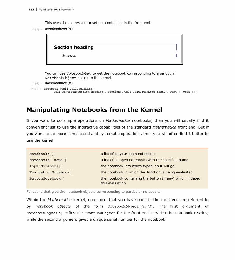
This uses the expression to set up a notebook in the front end.

In[5]:= NotebookPut@%D

You can use NotebookGet to get the notebook corresponding to a particular NotebookObject back into the kernel.

In[6]:= NotebookGet@%D

Out[6]= Notebook@8Cell@CellGroupData@8Cell@TextData@Section headingD, SectionD, Cell@TextData@Some text.D, TextD<, OpenDD<D

Manipulating Notebooks from the Kernel

If you want to do simple operations on Mathematica notebooks, then you will usually find it

convenient just to use the interactive capabilities of the standard Mathematica front end. But if

you want to do more complicated and systematic operations, then you will often find it better to

use the kernel.

Notebooks@D a list of all your open notebooks

Notebooks@"name"D a list of all open notebooks with the specified name

InputNotebook@D the notebook into which typed input will go

EvaluationNotebook@D the notebook in which this function is being evaluated

ButtonNotebook@D the notebook containing the button (if any) which initiated this evaluation

Functions that give the notebook objects corresponding to particular notebooks.

Within the Mathematica kernel, notebooks that you have open in the front end are referred to

by notebook objects of the form NotebookObject@ fe, idD. The first argument of

NotebookObject specifies the FrontEndObject for the front end in which the notebook resides,

while the second argument gives a unique serial number for the notebook.


Here is a notebook named Example.nb.

This finds the corresponding notebook object in the front end.

In[1]:= Notebooks@"Example.nb"D

Out[1]= NotebookObject[<<Example.nb>>]

This gets the expression corresponding to the notebook into the kernel.

In[2]:= NotebookGet@First@%DD

Out[2]= Notebook[Cell[First Heading, Section], Cell[Second Heading, Section]]

This replaces every occurrence of the string "Section" by "Text".

In[3]:= % ê. "Section" -> "Text"

Out[3]= Notebook[Cell[First Heading, Text], Cell[Second Heading, Text]]

This creates a new modified notebook in the front end.

In[4]:= NotebookPut@%D

Out[4]= NotebookObject[<<Untitled-1.nb>>]

NotebookGet@objD get the notebook expression corresponding to the note -book object obj

NotebookPut@expr,objD replaces the notebook represented by the notebook object obj with one corresponding to expr

NotebookPut@exprD creates a notebook corresponding to expr and makes it the currently selected notebook in the front end

Exchanging whole notebook expressions between the kernel and front end.

If you want to do extensive manipulations on a particular notebook you will usually find it

convenient to use NotebookGet to get the whole notebook into the kernel as a single expres-

sion. But if instead you want to do a sequence of small operations on a notebook, then it is

often better to leave the notebook in the front end, and then to send specific commands from

the kernel to the front end to tell it what operations to do.


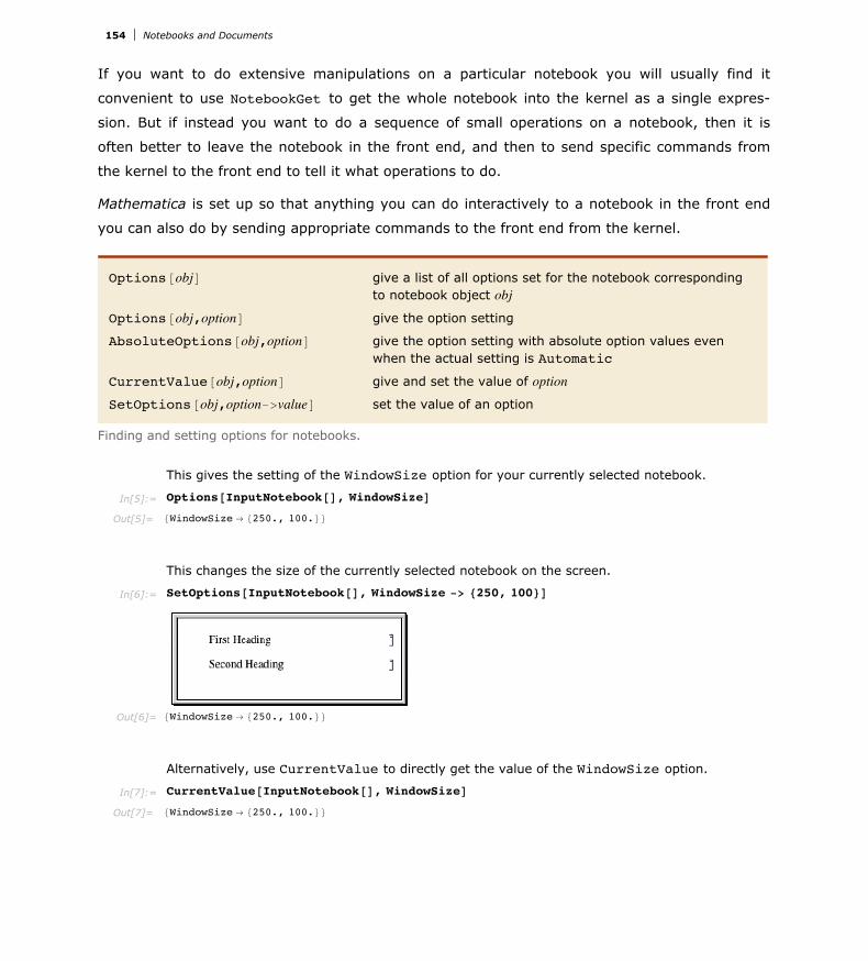
If you want to do extensive manipulations on a particular notebook you will usually find it

convenient to use NotebookGet to get the whole notebook into the kernel as a single expres-

sion. But if instead you want to do a sequence of small operations on a notebook, then it is

often better to leave the notebook in the front end, and then to send specific commands from

the kernel to the front end to tell it what operations to do.

Mathematica is set up so that anything you can do interactively to a notebook in the front end

you can also do by sending appropriate commands to the front end from the kernel.

Options@objD give a list of all options set for the notebook corresponding to notebook object obj

Options@obj,optionD give the option setting

AbsoluteOptions@obj,optionD give the option setting with absolute option values even when the actual setting is Automatic

CurrentValue@obj,optionD give and set the value of option

SetOptions@obj,option->valueD set the value of an option

Finding and setting options for notebooks.

This gives the setting of the WindowSize option for your currently selected notebook.

In[5]:= Options@InputNotebook@D, WindowSizeD

Out[5]= 8WindowSize Ø 8250., 100.<<

This changes the size of the currently selected notebook on the screen.

In[6]:= SetOptions@InputNotebook@D, WindowSize -> 8250, 100<D


Alternatively, use CurrentValue to directly get the value of the WindowSize option.

In[7]:= CurrentValue@InputNotebook@D, WindowSizeD



This changes the option using CurrentValue with a simple assignment.

In[8]:= CurrentValue@InputNotebook@D, WindowSizeD = 8400, 300<

Within any open notebook, the front end always maintains a current selection. The selection

can consist for example of a region of text within a cell or of a complete cell. Usually the selec-

tion is indicated on the screen by some form of highlighting. The selection can also be between

two characters of text, or between two cells, in which case it is usually indicated on the screen

by a vertical or horizontal insertion bar.

You can modify the current selection in an open notebook by issuing commands from the kernel.

SelectionMove@obj,Next,unitD move the current selection to make it be the next unit of the specified type

SelectionMove@obj,Previous,unitD move to the previous unit

SelectionMove@obj,After,unitD move to just after the end of the present unit of the specified type

SelectionMove@obj,Before,unitD move to just before the beginning of the present unit

SelectionMoveAobj,All,unitE extend the current selection to cover the whole unit of the specified type

Moving the current selection in a notebook.


Character individual character

Word word or other token

Expression complete subexpression

TextLine line of text

TextParagraph paragraph of text

GraphicsContents the contents of the graphic

Graphics graphic

CellContents the contents of the cell

Cell complete cell

CellGroup cell group

EvaluationCell cell associated with the current evaluation

ButtonCell cell associated with any button that initiated the evaluation

GeneratedCell cell generated by the current evaluation

Notebook complete notebook

Units used in specifying selections.

Here is a simple notebook.

This sets nb to be the notebook object corresponding to the current input notebook.

In[9]:= nb = InputNotebook@D;

This moves the current selection within the notebook to be the next word.

In[10]:= SelectionMove@nb, Next, WordD


This extends the selection to the complete first cell.

In[11]:= SelectionMove@nb, All, CellD

This puts the selection at the end of the whole notebook.

In[12]:= SelectionMove@nb, After, NotebookD

NotebookFind@obj,dataD move the current selection to the next occurrence of the specified data in a notebook

NotebookFind@obj,data,PreviousD move to the previous occurrence

NotebookFindAobj,data,AllE make the current selection cover all occurrences

NotebookFind@obj,data,dir,elemsD search in the specified elements of each cell, going in direction dir

NotebookFindAobj,"text",IgnoreCase->TrueE

do not distinguish uppercase and lowercase letters in text

Searching the contents of a notebook.

This moves the current selection to the position of the previous occurrence of the word cell.

In[13]:= NotebookFind@nb, "cell", PreviousD


The letter a does not appear in the current notebook, so $Failed is returned, and the selection is not moved.

In[14]:= NotebookFind@nb, "a", NextD

Out[14]= $Failed

CellContents contents of each cell

CellStyle the name of the style for each cell

CellLabel the label for each cell

CellTags tags associated with each cell

8elem1,elem2,…< several kinds of elements

Possible elements of cells to be searched by NotebookFind.

In setting up large notebooks, it is often convenient to insert tags which are not usually dis-

played, but which mark particular cells in such a way that they can be found using

NotebookFind. You can set up tags for cells either interactively in the front end, or by explicitly

setting the CellTags option for a cell.

NotebookLocate@"tag"D locate and select cells with the specified tag in the current notebook

NotebookLocate@8" file","tag"<D open another notebook if necessary

Globally locating cells in notebooks.

NotebookLocate is typically the underlying function that Mathematica calls when you follow a

hyperlink in a notebook. The Insert Hyperlink menu item sets up the appropriate

NotebookLocate as part of the script for a particular hyperlink button.


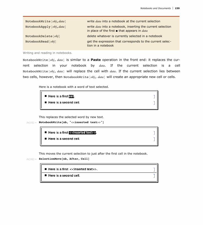
NotebookWrite@obj,dataD write data into a notebook at the current selection

NotebookApply@obj,dataD write data into a notebook, inserting the current selection in place of the first É that appears in data

NotebookDelete@objD delete whatever is currently selected in a notebook

NotebookRead@objD get the expression that corresponds to the current selec -tion in a notebook

Writing and reading in notebooks.

NotebookWrite@obj, dataD is similar to a Paste operation in the front end: it replaces the cur-

rent selection in your notebook by data. If the current selection is a cell

NotebookWrite@obj, dataD will replace the cell with data. If the current selection lies between

two cells, however, then NotebookWrite@obj, dataD will create an appropriate new cell or cells.

Here is a notebook with a word of text selected.

This replaces the selected word by new text.

In[15]:= NotebookWrite@nb, "<<inserted text>>"D

This moves the current selection to just after the first cell in the notebook.

In[16]:= SelectionMove@nb, After, CellD


This now inserts a text cell after the first cell in the notebook.

In[17]:= NotebookWrite@nb, Cell@"This cell contains text.", "Text"DD

This makes the current selection be the next cell in the notebook.

In[18]:= SelectionMove@nb, Next, CellD

This reads the current selection, returning it as an expression in the kernel.

In[19]:= NotebookRead@nbD

Out[19]= Cell@Here is a second one., SectionD

NotebookWrite@obj, dataD just discards the current selection and replaces it with data. But

particularly if you are setting up palettes, it is often convenient first to modify data by inserting

the current selection somewhere inside it. You can do this using selection placeholders and

NotebookApply. The first time the character "É", entered as î @SelectionPlaceholderD or Esc

splEsc, appears anywhere in data, NotebookApply will replace this character by the current

selection.


Here is a simple notebook with the current selection being the contents of a cell.


This replaces the current selection by a string that contains a copy of its previous form.

In[21]:= NotebookApply@nb, "x + 1êÉ"D

SelectionEvaluate@objD evaluate the current selection in place

SelectionCreateCell@objD create a new cell containing just the current selection

SelectionEvaluateCreateCell@objD

evaluate the current selection and create a new cell for the result

SelectionAnimate@objD animate graphics in the current selection

SelectionAnimate@obj,tD animate graphics for t seconds

Operations on the current selection.

This makes the current selection be the whole contents of the cell.

In[22]:= SelectionMove@nb, All, CellContentsD

This evaluates the current selection in place.

In[23]:= SelectionEvaluate@nbD

SelectionEvaluate allows you to take material from a notebook and send it through the kernel

for evaluation. On its own, however, SelectionEvaluate always overwrites the material you

took. But by using functions like SelectionCreateCell you can maintain a record of the

sequence of forms that are generated~just like in a standard Mathematica session.

This makes the current selection be the whole cell.


This makes the current selection be the whole cell.


This creates a new cell, and copies the current selection into it.

In[25]:= SelectionCreateCell@nbD

This wraps Factor around the contents of the current cell.

In[26]:= NotebookApply@nb, "Factor@ÉD"D

This evaluates the contents of the current cell, and creates a new cell to give the result.

In[27]:= SelectionEvaluateCreateCell@nbD

Functions like NotebookWrite and SelectionEvaluate by default leave the current selection

just after whatever material they insert into your notebook. You can then always move the

SelectionMove. But functions like NotebookWrite and

SelectionEvaluate can also take an additional argument which specifies where the current

selection should be left after they do their work.


Functions like NotebookWrite and SelectionEvaluate

selection by explicitly using SelectionMove. But functions like NotebookWrite and

SelectionEvaluate can also take an additional argument which specifies where the current

selection should be left after they do their work.

NotebookWrite@obj,data,selD write data into a notebook, leaving the current selection as specified by sel

NotebookApply@obj,data,selD write data replacing É by the previous current selection, then leaving the current selection as specified by sel

SelectionEvaluate@obj,selD evaluate the current selection, making the new current selection be as specified by sel

SelectionCreateCell@obj,selD create a new cell containing just the current selection, and make the new current selection be as specified by sel

SelectionEvaluateCreateCell@obj,selD

evaluate the current selection, make a new cell for the result, and make the new current selection be as specified by sel

Performing operations and specifying what the new current selection should be.

After immediately after whatever material is inserted (default)

Before immediately before whatever material is inserted

All the inserted material itself

Placeholder the first É in the inserted material

None leave the current selection unchanged

Specifications for the new current selection.

Here is a blank notebook.


This writes 10! into the notebook, making the current selection be what was written.

In[29]:= NotebookWrite@nb, "10!", AllD


This evaluates the current selection, creating a new cell for the result, and making the current selection be the whole of the result.

In[30]:= SelectionEvaluateCreateCell@nb, AllD

This wraps FactorInteger around the current selection.

In[31]:= NotebookApply@nb, "FactorInteger@ÉD", AllD

This evaluates the current selection, leaving the selection just before the result.

In[32]:= SelectionEvaluate@nb, BeforeD

This now inserts additional text at the position of the current selection.

In[33]:= NotebookWrite@nb, "a = "D

Options@obj,optionD find the value of an option for a complete notebook

Options@NotebookSelection@objD,optionD

find the value for the current selection

SetOptions@obj,option->valueD set the value of an option for a complete notebook

SetOptions@NotebookSelection@objD,option->valueD

set the value for the current selection

Finding and setting options for whole notebooks and for the current selection.


Make the current selection be a complete cell.


Put a frame around the cell that is the current selection.

In[35]:= SetOptions@NotebookSelection@nbD, CellFrame -> TrueD

CreateWindow@D create a new notebook

CreateWindow@optionsD create a notebook with specified options

NotebookOpen@"name"D open an existing notebook

NotebookOpen@"name",optionsD open a notebook with specified notebook options

SetSelectedNotebook@objD make the specified notebook the selected one

NotebookPrint@objD send a notebook to your printer

NotebookPrint@obj," file"D send a PostScript version of a notebook to a file

NotebookPrint@obj,"!command"D send a PostScript version of a notebook to an external command

NotebookSave@objD save the current version of a notebook in a file

NotebookSave@obj," file"D save the notebook in a file with the specified name

NotebookClose@objD close a notebook

Operations on whole notebooks.

If you call CreateWindow@D a new empty notebook will appear on your screen.

By executing commands like SetSelectedNotebook and NotebookOpen, you tell the Mathemat-

ica front end to change the windows you see. Sometimes you may want to manipulate a note-

book without ever having it displayed on the screen. You can do this by using the option setting

Visible -> False in NotebookOpen or CreateWindow.


Manipulating the Front End from the Kernel

$FrontEnd the front end currently in use

OptionsA$FrontEnd,optionE the setting for a global option in the front end

AbsoluteOptionsA$FrontEnd,optionE

the absolute setting for an option

SetOptionsA$FrontEnd,option->valueE

reset an option in the front end

CurrentValueA$FrontEnd, optionE return option value, and also allow setting of option when used as the left-hand side of an assignment

Manipulating global options in the front end.

Just like cells and notebooks, the complete Mathematica front end has various options, which

you can look at and manipulate from the kernel.

This gives the object corresponding to the front end currently in use.

In[1]:= $FrontEnd

Out[1]= Ü FrontEndObject Ü

This gives the current directory used by the front end for notebook files.

In[2]:= Options@$FrontEnd, NotebookBrowseDirectoryD

Out[2]= 9NotebookBrowseDirectory Ø C:\Documents and Settings\All Users\Documents=

option default valueNotebookBrowseDirectory (system

dependent)the default directory for opening and saving notebook files

NotebookPath (system dependent)

the path to search when trying to open notebooks

Language "English" default language for textMessageOptions (list of settings) how to handle various help and warning

messages

A few global options for the Mathematica front end.

By using NotebookWrite you can effectively input to the front end any ordinary text that you

can enter on the keyboard. FrontEndTokenExecute allows you to send from the kernel any

command that the front end can execute. These commands include both menu items and con-

trol sequences.


By using NotebookWrite you can effectively input to the front end any ordinary text that you

can enter on the keyboard. FrontEndTokenExecute allows you to send from the kernel any

command that the front end can execute. These commands include both menu items and con-

trol sequences.

FrontEndTokenExecute@"name"D execute a named command in the front end

Executing a named command in the front end.

"Indent" indent all selected lines by one tab

"NotebookStatisticsDialog" display statistics about the current notebook

"OpenCloseGroup" toggle a cell group between open and closed

"CellSplit" split a cell in two at the current insertion point

"DuplicatePreviousInput" create a new cell which is a duplicate of the nearest input cell above

"FindDialog" bring up the Find dialog

"ColorSelectorDialog" bring up the Color Selector dialog

"GraphicsAlign" align selected graphics

"CompleteSelection" complete the command name that is the current selection

A few named commands that can be given to the front end. These commands usually correspond to menu items.

Front End Tokens

Front end tokens let you perform kernel commands that would normally be done using the

menus. Front end tokens are particularly convenient for writing programs to manipulate

notebooks.

FrontEndToken is a kernel command that identifies its argument as a front end token.

FrontEndExecute is a kernel command that sends its argument to the front end for execution.

For example, the following command creates a new notebook.

In[10]:= FrontEndExecute@FrontEndToken@"New"DD

FrontEndExecute can take a list as its argument, allowing you to execute multiple tokens in a

single evaluation. When you evaluate the following command, the front end creates a new

notebook and then pastes the contents of the clipboard into that notebook.

In[9]:= FrontEndExecute@8FrontEndToken@"New"D, FrontEndToken@"Paste"D<D

Simple and Compound Front End Tokens


Simple and Compound Front End Tokens

Front end tokens are divided into two classes: simple tokens and compound tokens that take

parameters.

Simple Tokens

For simple tokens, FrontEndToken can have one or two arguments.

If FrontEndToken has one argument, the token operates on the input notebook. The following

examples use the front end token "Save". The result is the same as using File Save.

In[12]:= FrontEndExecute@FrontEndToken@"Save"DD

With two arguments, the arguments of FrontEndToken must be a NotebookObject and a front

end token. For example, to save the notebook containing the current evaluation, the first argu-

ment of FrontEndToken is the notebook object EvaluationNotebook , and the second argu-

ment is the front end token "Save".

In[3]:= FrontEndExecute@FrontEndToken@FrontEnd`EvaluationNotebook@D, "Save"DD

You can execute a simple, one-argument front end token with the command

FrontEndTokenExecute@tokenD. This is equivalent to FrontEndExecute@FrontEndToken@tokenDD.

For example, the following command will save the input notebook.

In[5]:= FrontEndTokenExecute@"Save"D

Compound Tokens

Compound tokens have a token parameter that controls some aspect of their behavior. For a

compound token, the three arguments of FrontEndToken must be a NotebookObject, the front

end token, and the selected token parameter.

For example, this saves the selected notebook as plain text.

In[6]:= FrontEndExecute@8FrontEndToken@FrontEnd`InputNotebook@D, "SaveRenameSpecial", "Text"D<D


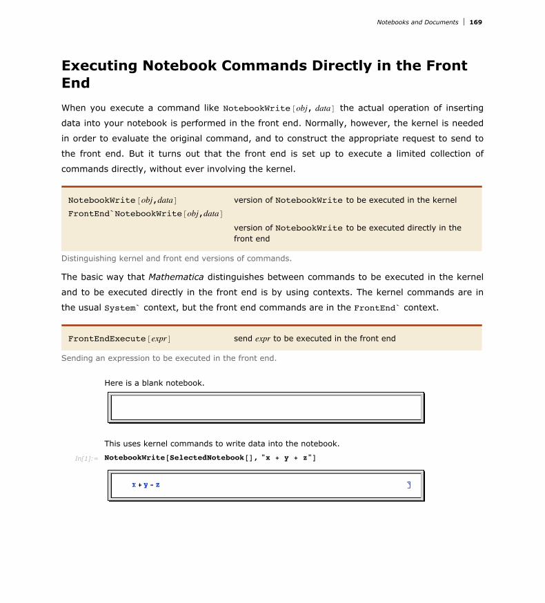
Executing Notebook Commands Directly in the Front End

When you execute a command like NotebookWrite@obj, dataD the actual operation of inserting

data into your notebook is performed in the front end. Normally, however, the kernel is needed

in order to evaluate the original command, and to construct the appropriate request to send to

the front end. But it turns out that the front end is set up to execute a limited collection of

commands directly, without ever involving the kernel.

NotebookWrite@obj,dataD version of NotebookWrite to be executed in the kernel

FrontEnd`NotebookWrite@obj,dataD

version of NotebookWrite to be executed directly in the front end

Distinguishing kernel and front end versions of commands.

The basic way that Mathematica distinguishes between commands to be executed in the kernel

and to be executed directly in the front end is by using contexts. The kernel commands are in

the usual System` context, but the front end commands are in the FrontEnd` context.

FrontEndExecute@exprD send expr to be executed in the front end

Sending an expression to be executed in the front end.

Here is a blank notebook.

This uses kernel commands to write data into the notebook.

In[1]:= NotebookWrite@SelectedNotebook@D, "x + y + z"D


In the kernel, these commands do absolutely nothing.

In[2]:= FrontEnd`NotebookWrite@FrontEnd`SelectedNotebook@D, "a + b + c + d"D

If they are sent to the front end, however, they cause data to be written into the notebook.

In[3]:= FrontEndExecute@%D

If you write sophisticated programs for manipulating notebooks, then you will have no choice

but to execute these programs primarily in the kernel. But for the kinds of operations typically

performed by simple buttons, you may find that it is possible to execute all the commands you

need directly in the front end~without the kernel even needing to be running.

The Structure of Cells

Cell@contents,"style"D a cell in a particular style

Cell@contents,"style1","style2",…D a cell with multiple styles

Cell@contents,"style",optionsD a cell with additional options set

Expressions corresponding to cells.

Here is a notebook containing a text cell and a Mathematica input cell.

Here are the expressions corresponding to these cells.

Here is a notebook containing a text cell with Mathematica input inside.


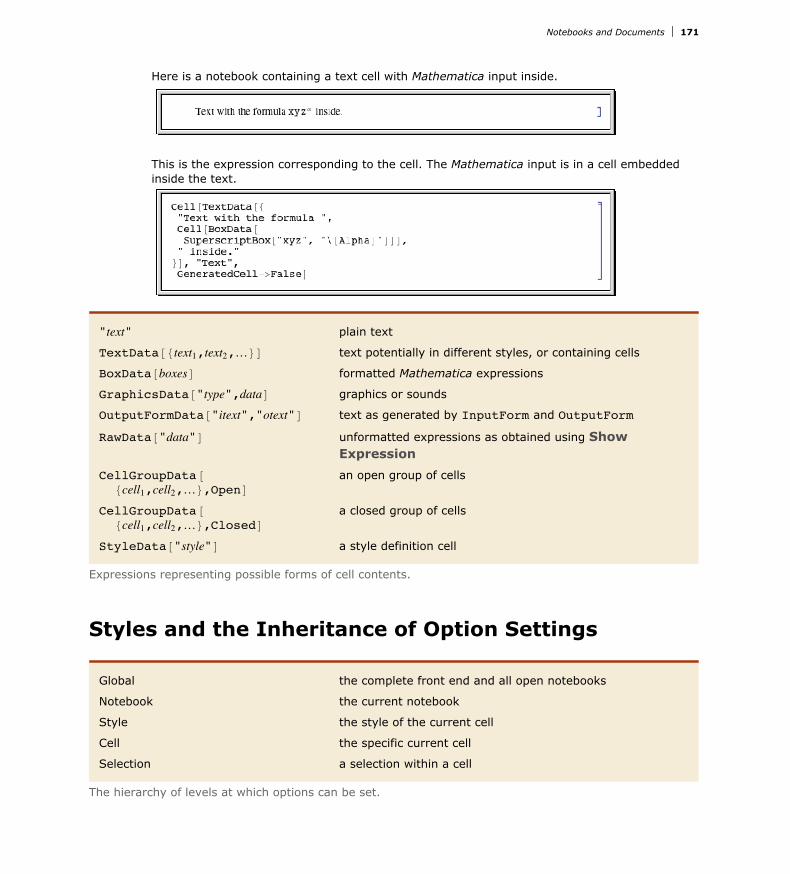
Here is a notebook containing a text cell with Mathematica input inside.

This is the expression corresponding to the cell. The Mathematica input is in a cell embedded inside the text.

"text" plain text

TextData@8text1,text2,…<D text potentially in different styles, or containing cells

BoxData@boxesD formatted Mathematica expressions

GraphicsData@"type",dataD graphics or sounds

OutputFormData@"itext","otext"D text as generated by InputForm and OutputForm

RawData@"data"D unformatted expressions as obtained using Show Expression

CellGroupData@8cell1,cell2,…<,OpenD

an open group of cells

CellGroupData@8cell1,cell2,…<,ClosedD

a closed group of cells

StyleData@"style"D a style definition cell

Expressions representing possible forms of cell contents.

Styles and the Inheritance of Option Settings

Global the complete front end and all open notebooks

Notebook the current notebook

Style the style of the current cell

Cell the specific current cell

Selection a selection within a cell

The hierarchy of levels at which options can be set.

Here is a notebook containing three cells.


Here is a notebook containing three cells.

This is what happens when the setting CellFrame -> True is made specifically for the third cell.

This is what happens when the setting CellFrame -> True is made globally for the whole notebook.

This is what happens when the setting is made for the "Section" style.

In the standard notebook front end, you can check and set options at any level by using the

Option Inspector menu item. If you do not set an option at a particular level, then its value

will always be inherited from the level above. Thus, for example, if a particular cell does not set

the CellFrame option, then the value used will be inherited from its setting for the style of the

cell or for the whole notebook that contains the cell.


In the standard notebook front end, you can check and set options at any level by using the

Option Inspector menu item. If you do not set an option at a particular level, then its value

will always be inherited from the level above. Thus, for example, if a particular cell does not set

the CellFrame option, then the value used will be inherited from its setting for the style of the

cell or for the whole notebook that contains the cell.

As a result, if you set CellFrame -> True at the level of a whole notebook, then all the cells in

the notebook will have frames drawn around them~unless the style of a particular cell, or the

cell itself, explicitly overrides this setting.

† Choose the basic default styles for a notebook

† Choose the styles for screen and printing style environments

† Edit specific styles for the notebook

Ways to set up styles in a notebook.

Depending on what you intend to use your Mathematica notebook for, you may want to choose

different basic default styles for the notebook. In the standard notebook front end, you can do

this by selecting a different stylesheet in the Stylesheet menu or by using the Edit

Stylesheet menu item.

"StandardReport" styles for everyday work and for reports

"NaturalColor" styles for colorful presentation of everyday work

"Outline" styles for outlining ideas

"Notepad" styles for working with plain text documents

Some typical choices of basic default styles.

With each choice of basic default styles, the styles that are provided will change. Thus, for

example, the Notepad stylesheet provides a limited number of styles since it is designed to

work with plain text documents.


Here is a notebook that uses NaturalColor default styles.

option default valueScreenStyleEnvironment "Working" the style environment to use for display on

the screenPrintingStyleEnvironment "Printout" the style environment to use for printed

output

Options for specifying style environments.

Within a particular set of basic default styles, Mathematica allows for two different style environ-

ments: one for display on the screen, and another for output to a printer. The existence of

separate screen and printing style environments allows you to set up styles which are sepa-

rately optimized both for low-resolution display on a screen, and high-resolution printing.

"Working" onscreen working environment

"Presentation" onscreen environment for presentations

"Condensed" onscreen environment for maximum display density

"Slideshow" onscreen environment for displaying slides

"Printout" paper printout environment

Some typical settings for style environments.

The way that Mathematica actually sets up the definitions for styles is by using style definition

cells. These cells can either be given in separate stylesheet notebooks, or can be included in the

options of a specific notebook. In either case, you can access style definitions by using the Edit

Stylesheet menu item in the standard notebook front end.


The way that Mathematica actually sets up the definitions for styles is by using style definition

cells. These cells can either be given in separate stylesheet notebooks, or can be included in the

options of a specific notebook. In either case, you can access style definitions by using the Edit

Stylesheet menu item in the standard notebook front end.

Options for Cells

Mathematica provides a large number of options for cells. All of these options can be accessed

through the Option Inspector menu item in the front end. They can be set either directly at

the level of individual cells or at a higher level, to be inherited by individual cells.

option typical default value

CellDingbat None a dingbat to use to emphasize the cell

CellFrame False whether to draw a frame around the cell

Background None the background color for the cell

ShowCellBracket True whether to display the cell bracket

Magnification 1. the magnification at which to display the cell

CellOpen True whether to display the contents of the cell

Some basic cell display options.

This creates a cell in "Section" style with default settings for all options.

In[1]:= CellPrint@Cell@"A Heading", "Section"DD


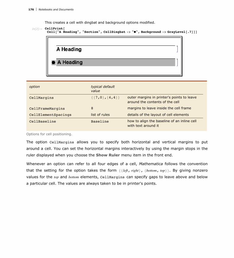
This creates a cell with dingbat and background options modified.

In[2]:= CellPrint@Cell@"A Heading", "Section", CellDingbat -> "Ê", Background -> [email protected]


CellMargins 887,0<,84,4<< outer margins in printer's points to leave around the contents of the cell

CellFrameMargins 8 margins to leave inside the cell frame

CellElementSpacings list of rules details of the layout of cell elements

CellBaseline Baseline how to align the baseline of an inline cell with text around it

Options for cell positioning.

The option CellMargins allows you to specify both horizontal and vertical margins to put

around a cell. You can set the horizontal margins interactively by using the margin stops in the

ruler displayed when you choose the Show Ruler menu item in the front end.

Whenever an option can refer to all four edges of a cell, Mathematica follows the convention

that the setting for the option takes the form 88left, right<, 8bottom, top<<. By giving nonzero

values for the top and bottom elements, CellMargins can specify gaps to leave above and below

a particular cell. The values are always taken to be in printer's points.


This leaves 50 points of space on the left of the cell, and 20 points above and below.

In[3]:= CellPrint@Cell@"First text", "Text", CellMargins -> 8850, 0<, 820, 20<<DD

Almost every aspect of Mathematica notebooks can be controlled by some option or another.

More detailed aspects are typically handled by "aggregate options" such as

CellElementSpacings. The settings for these options are lists of Mathematica rules, which

effectively give values for a sequence of suboptions. The names of these suboptions are usually

strings rather than symbols.

This shows the settings for all the suboptions associated with CellElementSpacings.

In[4]:= Options@SelectedNotebook@D, CellElementSpacingsD

Out[4]= 8CellElementSpacings Ø 8CellMinHeight Ø 12., ClosedCellHeight Ø 19.,ClosedGroupTopMargin Ø 4., GroupIconTopMargin Ø 3., GroupIconBottomMargin Ø 12.<<

Mathematica allows you to embed cells inside pieces of text. The option CellBaseline deter-

mines how such "inline cells" will be aligned vertically with respect to the text around them. In

direct analogy with the option BaselinePosition for a Grid, the option CellBaseline speci-

fies what aspect of the cell should be considered its baseline.

Here is a cell containing an inline formula. The baseline of the formula is aligned with the baseline of the text around it.

Here is a cell in which the bottom of the formula is aligned with the baseline of the text around it.

This alignment is specified using the CellBaseline -> Bottom setting.


This alignment is specified using the CellBaseline -> Bottom setting.


CellLabel "" a label for a cell

ShowCellLabel True whether to show the label for a cell

CellLabelAutoDelete True whether to delete the label if the cell is modified

CellTags 8< tags for a cell

ShowCellTags False whether to show tags for a cell

ConversionRules 8< rules for external conversions

Options for ancillary data associated with cells.

In addition to the actual contents of a cell, it is often useful to associate various kinds of ancil-

lary data with cells.

In a standard Mathematica session, cells containing successive lines of kernel input and output

are given labels of the form In@nD := and Out@nD =. The option ShowCellLabel determines

whether such labels should be displayed. CellLabelAutoDelete determines whether the label

on a cell should be removed if the contents of the cell are modified. Doing this ensures that

In@nD := and Out@nD = labels are only associated with unmodified pieces of kernel input and

output.

Cell tags are typically used to associate keywords or other attributes with cells, that can be

searched for using functions like NotebookFind. Destinations for hyperlinks in Mathematica

notebooks are usually implemented using cell tags.

The option ConversionRules allows you to give a list containing entries such as "TeX" -> data

which specify how the contents of a cell should be converted to external formats. This is particu-

larly relevant if you want to keep a copy of the original form of a cell that has been converted in

Mathematica notebook format from some external format.



Deletable True whether to allow a cell to be deleted interactively with the front end

Copyable True whether to allow a cell to be copied

Selectable True whether to allow the contents of a cell to be selected

Editable True whether to allow the contents of a cell to be edited

Deployed False whether the user interface in the cell is active

Options for controlling interactive operations on cells.

The options Deletable, Copyable, Selectable and Editable allow you to control what interac-

tive operations should be allowed on cells. By setting these options to False at the notebook

level, you can protect all the cells in a notebook.

Deployed allows you to treat the contents of a cell as if they were a user interface. In a user

interface, labels are typically not selectable and controls such as buttons can be used, but not

modified. Deployed can also be set on specific elements inside a cell so that, for example, the

output of Manipulate is always deployed even if the cell it is in has the Deployed option set to

False.


Evaluator "Local" the name of the kernel to use for evaluations

Evaluatable False whether to allow the contents of a cell to be evaluated

CellAutoOverwrite False whether to overwrite previous output when new output is generated

GeneratedCell False whether this cell was generated from the kernel

InitializationCell False whether this cell should automatically be evaluated when the notebook is opened

Options for evaluation.

Mathematica makes it possible to specify a different evaluator for each cell in a notebook. But

most often, the Evaluator option is set only at the notebook or global level, typically using the

Kernel Configuration Options menu item in the front end.


Mathematica makes it possible to specify a different evaluator for each cell in a notebook. But

most often, the Evaluator option is set only at the notebook or global level, typically using the

Kernel Configuration Options menu item in the front end.

The option CellAutoOverwrite is typically set to True for styles that represent Mathematica

output. Doing this means that when you reevaluate a particular piece of input, Mathematica will

automatically delete the output that was previously generated from that input, and will over-

write it with new output.

The option GeneratedCell is set whenever a cell is generated by an external request to the

front end rather than by an interactive operation within the front end. Thus, for example, any

cell obtained as an output or side effect from a kernel evaluation will have

GeneratedCell -> True. Cells generated by low-level functions designed to manipulate note-

books directly, such as NotebookWrite and NotebookApply, do not have the GeneratedCell

option set.


PageBreakAbove Automatic whether to put a page break just above a particular cell

PageBreakWithin Automatic whether to allow a page break within a particular cell

PageBreakBelow Automatic whether to put a page break just below a particular cell

GroupPageBreakWithin Automatic whether to allow a page break within a particular group of cells

Options for controlling page breaks when cells are printed.

When you display a notebook on the screen, you can scroll continuously through it. But if you

print the notebook out, you have to decide where page breaks will occur. A setting of

Automatic for a page break option tells Mathematica to make a page break if necessary; True

specifies that a page break should always be made, while False specifies that it should never

be.

Page breaks set using the PageBreakAbove and PageBreakBelow options also determine the

breaks between slides in a slide show. When creating a slide show, you will typically use a cell

with a special named style to determine where each slide begins. This named style will have

one of the page-breaking options set on it.

Additional functionality related to this tutorial has been introduced in subsequent versions of Mathematica. For the latest information, see Text Styling.


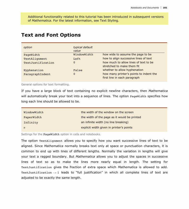
Additional functionality related to this tutorial has been introduced in subsequent versions of Mathematica. For the latest information, see Text Styling.

Text and Font Options


PageWidth WindowWidth how wide to assume the page to beTextAlignment Left how to align successive lines of textTextJustification 0 how much to allow lines of text to be

stretched to make them fitHyphenation False whether to allow hyphenationParagraphIndent 0 how many printer’s points to indent the

first line in each paragraph

General options for text formatting.

If you have a large block of text containing no explicit newline characters, then Mathematica

will automatically break your text into a sequence of lines. The option PageWidth specifies how

long each line should be allowed to be.

WindowWidth the width of the window on the screen

PaperWidth the width of the page as it would be printed

Infinity an infinite width (no line breaking)

n explicit width given in printer’s points

Settings for the PageWidth option in cells and notebooks.

The option TextAlignment allows you to specify how you want successive lines of text to be

aligned. Since Mathematica normally breaks text only at space or punctuation characters, it is

common to end up with lines of different lengths. Normally the variation in lengths will give

your text a ragged boundary. But Mathematica allows you to adjust the spaces in successive

lines of text so as to make the lines more nearly equal in length. The setting for

TextJustification gives the fraction of extra space which Mathematica is allowed to add.

TextJustification -> 1 leads to “full justification” in which all complete lines of text are

adjusted to be exactly the same length.


Left aligned on the left

Right aligned on the right

Center centered

x aligned at a position x running from -1 to +1 across the page

Settings for the TextAlignment option.

Here is text with TextAlignment -> Left and TextJustification -> 0.

With TextAlignment -> Center the text is centered.

TextJustification -> 1 adjusts word spacing so that both the left and right edges line up.

TextJustification -> 0.5 reduces the degree of raggedness, but does not force the left and right edges to be precisely lined up.


With Hyphenation -> True the text is hyphenated.

When you enter a block of text in a Mathematica notebook, Mathematica will treat any explicit

newline characters that you type as paragraph breaks. The option ParagraphIndent allows you

to specify how much you want to indent the first line in each paragraph. By giving a negative

setting for ParagraphIndent, you can make the first line stick out to the left relative to subse-

quent lines.

LineSpacing->9c,0= leave space so that the total height of each line is c times the height of its contents

LineSpacing->90,n= make the total height of each line exactly n printer’s points

LineSpacing->9c,n= make the total height c times the height of the contents plus n printer’s points

ParagraphSpacing->9c,0= leave an extra space of c times the height of the font before the beginning of each paragraph

ParagraphSpacing->90,n= leave an extra space of exactly n printer’s points before the beginning of each paragraph

ParagraphSpacing->9c,n= leave an extra space of c times the height of the font plus n printer’s points

Options for spacing between lines of text.

Here is some text with the default setting LineSpacing -> 81, 1<, which inserts just 1 printer’s point of extra space between successive lines.


With LineSpacing -> 81, 5< the text is “looser”.

LineSpacing -> 82, 0< makes the text double-spaced.

With LineSpacing -> 81, -2< the text is tight.


FontFamily "Courier" the family of font to useFontSubstitutions 8< a list of substitutions to try for font family

namesFontSize 12 the maximum height of characters in

printer’s pointsFontWeight "Bold" the weight of characters to useFontSlant "Plain" the slant of characters to useFontTracking "Plain" the horizontal compression or expansion of

charactersFontColor GrayLevel@0D the color of charactersBackground GrayLevel@1D the color of the background for each

character

Options for fonts.


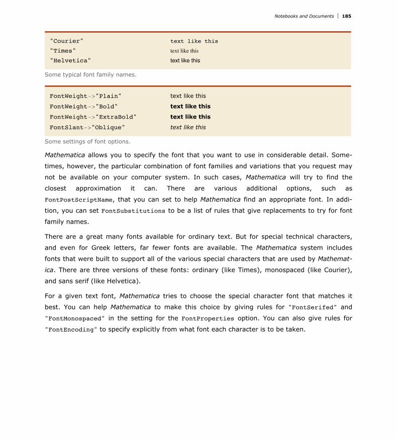
"Courier" text like this

"Times" text like this

"Helvetica" text like this

Some typical font family names.

FontWeight->"Plain" text like this

FontWeight->"Bold" text like this

FontWeight->"ExtraBold" text like this

FontSlant->"Oblique" text like this

Some settings of font options.

Mathematica allows you to specify the font that you want to use in considerable detail. Some-

times, however, the particular combination of font families and variations that you request may

not be available on your computer system. In such cases, Mathematica will try to find the

closest approximation it can. There are various additional options, such as

FontPostScriptName, that you can set to help Mathematica find an appropriate font. In addi-

tion, you can set FontSubstitutions to be a list of rules that give replacements to try for font

family names.

There are a great many fonts available for ordinary text. But for special technical characters,

and even for Greek letters, far fewer fonts are available. The Mathematica system includes

fonts that were built to support all of the various special characters that are used by Mathemat-

ica. There are three versions of these fonts: ordinary (like Times), monospaced (like Courier),

and sans serif (like Helvetica).

For a given text font, Mathematica tries to choose the special character font that matches it

best. You can help Mathematica to make this choice by giving rules for "FontSerifed" and

"FontMonospaced" in the setting for the FontProperties option. You can also give rules for

"FontEncoding" to specify explicitly from what font each character is to be taken.


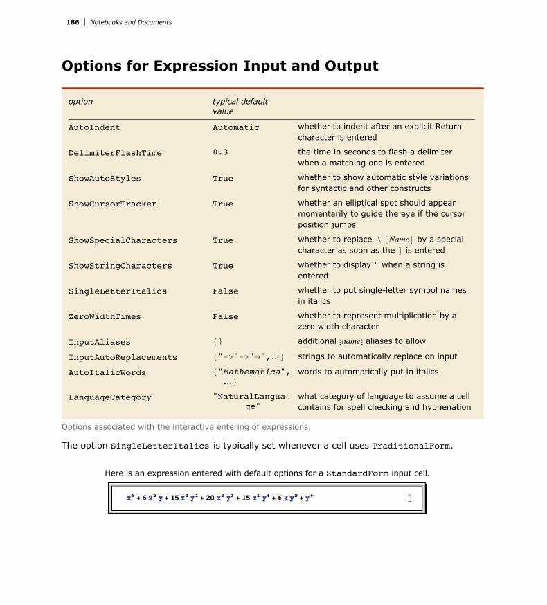
Options for Expression Input and Output


AutoIndent Automatic whether to indent after an explicit Return character is entered

DelimiterFlashTime 0.3 the time in seconds to flash a delimiter when a matching one is entered

ShowAutoStyles True whether to show automatic style variations for syntactic and other constructs

ShowCursorTracker True whether an elliptical spot should appear momentarily to guide the eye if the cursor position jumps

ShowSpecialCharacters True whether to replace î @NameD by a special character as soon as the D is entered

ShowStringCharacters True whether to display " when a string is entered

SingleLetterItalics False whether to put single-letter symbol names in italics

ZeroWidthTimes False whether to represent multiplication by a zero width character

InputAliases 8< additional ÇnameÇ aliases to allow

InputAutoReplacements 8"->"->"Ø",…< strings to automatically replace on input

AutoItalicWords 8"Mathematica",…<

words to automatically put in italics

LanguageCategory "NaturalLanguaÖge"

what category of language to assume a cell contains for spell checking and hyphenation

Options associated with the interactive entering of expressions.

The option SingleLetterItalics is typically set whenever a cell uses TraditionalForm.

Here is an expression entered with default options for a StandardForm input cell.


Here is the same expression entered in a cell with SingleLetterItalics -> True and ZeroWidthTimes -> True.

Built into Mathematica are a large number of aliases for common special characters.

InputAliases allows you to add your own aliases for further special characters or for any other

kind of Mathematica input. A rule of the form "name" -> expr specifies that ÇnameÇ should immedi-

ately be replaced on input by expr.

Aliases are delimited by explicit Esc characters. The option InputAutoReplacements allows you

to specify that certain kinds of input sequences should be immediately replaced even when they

have no explicit delimiters. By default, for example, -> is immediately replaced by Ø. You can

give a rule of the form "seq" -> "rhs" to specify that whenever seq appears as a token in your

input, it should immediately be replaced by rhs.

"NaturalLanguage" human natural language such as English

"Mathematica" Mathematica input

"Formula" mathematical formula

None do no spell checking or hyphenation

Settings for LanguageCategory to control spell checking and hyphenation.

The option LanguageCategory allows you to tell Mathematica what type of contents it should

assume cells have. This determines how spelling and structure should be checked, and how

hyphenation should be done.


StructuredSelection False whether to allow only complete subexpres -sions to be selected

DragAndDrop False whether to allow drag-and-drop editing

Options associated with interactive manipulation of expressions.

Mathematica normally allows you to select any part of an expression that you see on the

screen. Occasionally, however, you may find it useful to get Mathematica to allow only selec-

tions which correspond to complete subexpressions. You can do this by setting the option

StructuredSelection -> True.

Here is an expression with a piece selected.


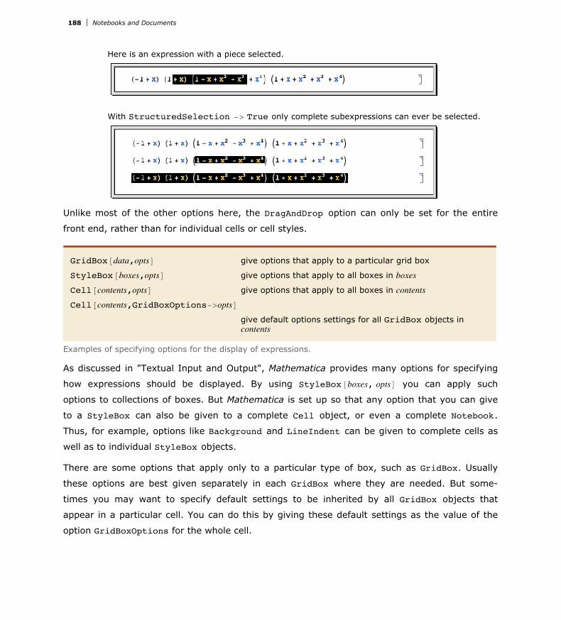
Here is an expression with a piece selected.

With StructuredSelection -> True only complete subexpressions can ever be selected.

Unlike most of the other options here, the DragAndDrop option can only be set for the entire

front end, rather than for individual cells or cell styles.

GridBox@data,optsD give options that apply to a particular grid box

StyleBox@boxes,optsD give options that apply to all boxes in boxes

Cell@contents,optsD give options that apply to all boxes in contents

Cell@contents,GridBoxOptions->optsD

give default options settings for all GridBox objects in contents

Examples of specifying options for the display of expressions.

As discussed in "Textual Input and Output", Mathematica provides many options for specifying

how expressions should be displayed. By using StyleBox@boxes, optsD you can apply such

options to collections of boxes. But Mathematica is set up so that any option that you can give

to a StyleBox can also be given to a complete Cell object, or even a complete Notebook.

Thus, for example, options like Background and LineIndent can be given to complete cells as

well as to individual StyleBox objects.

There are some options that apply only to a particular type of box, such as GridBox. Usually

these options are best given separately in each GridBox where they are needed. But some-

times you may want to specify default settings to be inherited by all GridBox objects that

appear in a particular cell. You can do this by giving these default settings as the value of the

option GridBoxOptions for the whole cell.

For most box types named XXXBox, Mathematica provides a cell option XXXBoxOptions that

allows you to specify the default options settings for that type of box. Box types which take

options can also have their options set in a stylesheet by defining the XXX style. The stylesheets

which come with Mathematica define many such styles.


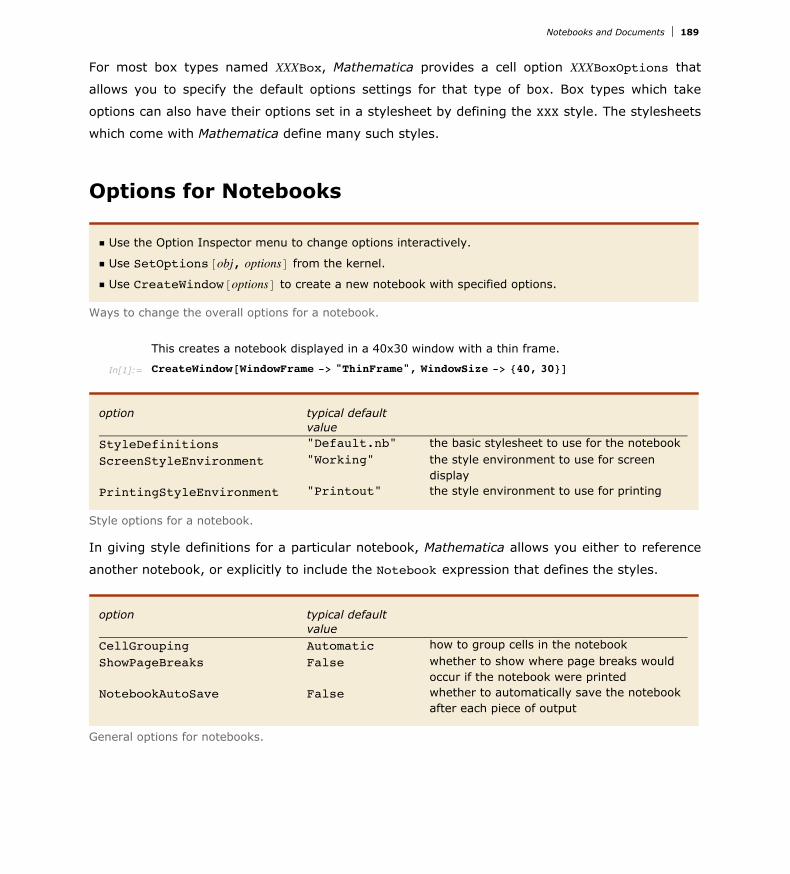
For most box types named XXXBox, Mathematica provides a cell option XXXBoxOptions that

allows you to specify the default options settings for that type of box. Box types which take

options can also have their options set in a stylesheet by defining the XXX style. The stylesheets

which come with Mathematica define many such styles.

Options for Notebooks

† Use the Option Inspector menu to change options interactively.

† Use SetOptions@obj, optionsD from the kernel.

† Use CreateWindow@optionsD to create a new notebook with specified options.

Ways to change the overall options for a notebook.

This creates a notebook displayed in a 40x30 window with a thin frame.

In[1]:= CreateWindow@WindowFrame -> "ThinFrame", WindowSize -> 840, 30<D


StyleDefinitions "Default.nb" the basic stylesheet to use for the notebookScreenStyleEnvironment "Working" the style environment to use for screen

displayPrintingStyleEnvironment "Printout" the style environment to use for printing

Style options for a notebook.

In giving style definitions for a particular notebook, Mathematica allows you either to reference

another notebook, or explicitly to include the Notebook expression that defines the styles.


CellGrouping Automatic how to group cells in the notebookShowPageBreaks False whether to show where page breaks would

occur if the notebook were printedNotebookAutoSave False whether to automatically save the notebook

after each piece of output

General options for notebooks.


With CellGrouping -> Automatic, cells are automatically grouped based on their style.

With CellGrouping -> Manual, you have to group cells by hand.


DefaultNewCellStyle "Input" the default style for new cells created in the notebook

DefaultDuplicateCellStyle "Input" the default style for cells created by auto -matic duplication of existing cells

Options specifying default styles for cells created in a notebook.

Mathematica allows you to take any cell option and set it at the notebook level, thereby specify-

ing a global default for that option throughout the notebook.


Editable True whether to allow cells in the notebook to be edited

Selectable True whether to allow cells to be selectedDeletable True whether to allow cells to be deletedShowSelection True whether to show the current selection

highlightedBackground GrayLevel@1D what background color to use for the

notebookMagnification 1 at what magnification to display the

notebookPageWidth WindowWidth how wide to allow the contents of cells to be

A few cell options that are often set at the notebook level.

Here is a notebook with the Background option set at the notebook level.


Here is a notebook with the Background option set at the notebook level.


Visible True whether the window should be visible on the screen

WindowSize 9Automatic,Automatic=

the width and height of the window in printer’s points

WindowMargins Automatic the margins to leave around the window when it is displayed on the screen

WindowFrame "Normal" the type of frame to draw around the window

WindowElements 8"StatusArea",…<

elements to include in the window

WindowTitle Automatic what title should be displayed for the window

WindowMovable True whether to allow the window to be moved around on the screen

WindowFloating False whether the window should always float on top of other windows

WindowClickSelect True whether the window should become selected if you click in it

DockedCells 8< a list of cells specifying the content of a docked area at the top of the window

Characteristics of the notebook window.

WindowSize allows you to specify how large you want a window to be; WindowMargins allows

you to specify where you want the window to be placed on your screen. The setting

WindowMargins -> 88left, right<, 8bottom, top<< gives the margins in pixels to leave around your

window on the screen. Often only two of the margins will be set explicitly; the others will be

Automatic, indicating that these margins will be determined from the particular size of screen

that you use.

WindowClickSelect is the principal option that determines whether a window acts like a

palette. Palettes are generally windows with content that acts upon other windows, rather than

windows which need to be selected for their own ends. Palettes also generally have a collection

of other option settings such as WindowFloating -> True and WindowFrame -> "Palette".

DockedCells allows you to specify any content that you want to stay at the top of a window

and never scroll offscreen. A typical use of the DockedCells option is to define a custom tool-

bar. Many default stylesheets have the DockedCells option defined in certain environments to

create toolbars for purposes such as presenting slideshows and editing package files.


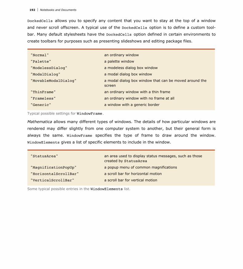
DockedCells allows you to specify any content that you want to stay at the top of a window

and never scroll offscreen. A typical use of the DockedCells option is to define a custom tool-

bar. Many default stylesheets have the DockedCells option defined in certain environments to

create toolbars for purposes such as presenting slideshows and editing package files.

"Normal" an ordinary window

"Palette" a palette window

"ModelessDialog" a modeless dialog box window

"ModalDialog" a modal dialog box window

"MovableModalDialog" a modal dialog box window that can be moved around the screen

"ThinFrame" an ordinary window with a thin frame

"Frameless" an ordinary window with no frame at all

"Generic" a window with a generic border

Typical possible settings for WindowFrame .

Mathematica allows many different types of windows. The details of how particular windows are

rendered may differ slightly from one computer system to another, but their general form is

always the same. WindowFrame specifies the type of frame to draw around the window.

WindowElements gives a list of specific elements to include in the window.

"StatusArea" an area used to display status messages, such as those created by StatusArea

"MagnificationPopUp" a popup menu of common magnifications

"HorizontalScrollBar" a scroll bar for horizontal motion

"VerticalScrollBar" a scroll bar for vertical motion

Some typical possible entries in the WindowElements list.


Here is a window with a status area and horizontal scroll bar, but no magnification popup or vertical scroll bar.

Global Options for the Front End

In the standard notebook front end, Mathematica allows you to set a large number of global

options. The values of all these options are by default saved in a “preferences file”, and are

automatically reused when you run Mathematica again. These options include all the settings

which can be made using the Preferences dialog.

style definitions default style definitions to use for new notebooks

file locations directories for finding notebooks and system files

data export options how to export data in various formats

character encoding options how to encode special characters

language options what language to use for text

message options how to handle messages generated by Mathematica

dialog settings choices made in dialog boxes

system configuration private options for specific computer systems

Some typical categories of global options for the front end.

You can access global front end options from the kernel by using Options@$FrontEnd, nameD.

But more often, you will want to access these options interactively using the Option Inspector in

the front end.


Mathematical and Other Notation

Mathematical Notation in Notebooks

If you use a text-based interface to Mathematica, then the input you give must consist only of

characters that you can type directly on your computer keyboard. But if you use a notebook

interface then other kinds of input become possible.

There are palettes provided which operate like extensions of your keyboard, and which have

buttons that you can click to enter particular forms. You can access standard palettes using the

Palettes menu.

Clicking the p button in this palette will enter a Pi into your notebook.


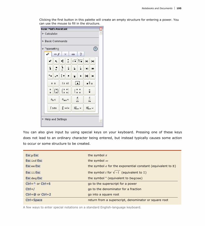
Clicking the first button in this palette will create an empty structure for entering a power. You can use the mouse to fill in the structure.

You can also give input by using special keys on your keyboard. Pressing one of these keys

does not lead to an ordinary character being entered, but instead typically causes some action

to occur or some structure to be created.

Esc pEsc the symbol p

Esc infEsc the symbol ¶

Esc eeEsc the symbol ‰ for the exponential constant (equivalent to E)

Esc iiEsc the symbol Â for -1 (equivalent to I)

Esc degEsc the symbol ° (equivalent to Degree)

Ctrl+^ or Ctrl+6 go to the superscript for a power

Ctrl+/ go to the denominator for a fraction

Ctrl+@ or Ctrl+2 go into a square root

Ctrl+Space return from a superscript, denominator or square root

A few ways to enter special notations on a standard English-language keyboard.

Here is a computation entered using ordinary characters on a keyboard.


Here is a computation entered using ordinary characters on a keyboard.

In[1]:= N@Pi^2 ê 6D

Out[1]= 1.64493

Here is the same computation entered using a palette or special keys.

In[2]:= NBp2

6F

Out[2]= 1.64493

Here is an actual sequence of keys that can be used to enter the input.

In[3]:= N[ Esc pEsc Ctrl+^ 2 Ctrl+Space Ctrl+/ 6 Ctrl+Space ]Out[3]= 1.64493

In a traditional computer language such as C, Fortran, Java or Perl, the input you give must

always consist of a string of ordinary characters that can be typed directly on a keyboard. But

the Mathematica language also allows you to give input that contains special characters, super-

scripts, built-up fractions, and so on.

The language incorporates many features of traditional mathematical notation. But you should

realize that the goal of the language is to provide a precise and consistent way to specify compu -

tations. And as a result, it does not follow all of the somewhat haphazard details of traditional

mathematical notation.

Nevertheless, as discussed in "Forms of Input and Output", it is always possible to get Mathemat-

ica to produce output that imitates every aspect of traditional mathematical notation. And it is

also possible for Mathematica to import text that uses such notation, and to some extent to

translate it into its own more precise language.

Mathematical Notation in Notebooks

If you use the notebook front end for Mathematica, then you can enter some of the operations

discussed here in special ways.


⁄i=iminimax f Sum@ f,8i,imin,imax<D sum

¤i=iminimax f Product@ f,8i,imin,imax<D product

Ÿ f „ x Integrate@ f,xD indefinite integral

Ÿxminxmax f „ x Integrate@ f,8x,xmin,xmax<D definite integral

∂x f D@ f,xD partial derivative

∂x,y f D@ f,x,yD multivariate partial derivative

Special and ordinary ways to enter mathematical operations in notebooks.

This one of the standard palettes for entering mathematical operations. When you click a button in the palette, the form shown in the button is inserted into your notebook, with the black square replaced by whatever you had selected in the notebook.


Esc sumEsc summation sign ⁄

Esc prodEsc product sign ¤

Esc intEsc integral sign Ÿ

Esc ddEsc special differential „ for use in integrals

Esc pdEsc partial derivative ∂

Ctrl+_ or Ctrl+- move to the subscript position or lower limit of an integral

Ctrl+^ or Ctrl+6 move to the superscript position or upper limit of an integral

Ctrl++ or Ctrl+= move to the underscript position or lower limit of a sum or product

Ctrl+& or Ctrl+7 move to the overscript position or upper limit of a sum or product

Ctrl+% or Ctrl+5 switch between upper and lower positions

Ctrl+Space return from upper or lower positions

Ways to enter special notations on a standard English-language keyboard.

You can enter an integral like this. Be sure to use the special differential „ entered as Esc ddEsc, not just an ordinary d.

In[1]:= ‡ xn „x

Out[1]= x1+n

1 + n

Here is the actual key sequence you type to get the input.

In[2]:= Esc intEsc x Ctrl+^ n Ctrl+Space Esc ddEsc x

Out[2]= x1+n

1 + n

When entering a sum, product or integral that has limits, you can create the first limit using the

standard control sequences for subscripts, superscripts, underscripts, or overscripts. However,

you must use Ctrl+% to create the second limit.

You can enter a sum like this.

In[3]:= ‚x=0

n

x

Out[3]=1

2n H1 + nL




In[4]:= Esc sumEsc Ctrl+= x=0 Ctrl+% n Ctrl+Space x

Out[4]=1

2n H1 + nL

Special Characters

Built into Mathematica are a large number of special characters intended for use in mathemati-

cal and other notation. "Listing of Named Characters" gives a complete listing.

Each special character is assigned a full name such as \[Infinity]. More common special

characters are also assigned aliases, such as Esc infEsc. You can set up additional aliases

using the InputAliases notebook option discussed in "Options for Expression Input and Out-

put".

For special characters that are supported in standard dialects of TeX, Mathematica also allows

you to use aliases based on TeX names. Thus, for example, you can enter \[Infinity] using

the alias Esc \infty Esc. Mathematica also supports aliases such as Esc¶Esc based on names

used in SGML and HTML.

Standard system software on many computer systems also supports special key combinations

for entering certain special characters. On a Macintosh, for example, Option+5 will produce ¶ in

most fonts. With the notebook front end Mathematica automatically allows you to use special

key combinations when these are available, and with a text-based interface you can get Mathe-

matica to accept such key combinations if you set an appropriate value for

$CharacterEncoding.

† Use a full name such as \[Infinity]

† Use an alias such as Esc infEsc

† Use a TeX alias such as Esc \infty Esc

† Use an SGML or HTML alias such as Esc¶Esc

† Click a button in a palette

† Use a special key combination supported by your computer system

Ways to enter special characters.

In a Mathematica notebook, you can use special characters just like you use standard keyboard

characters. You can include special characters both in ordinary text and in input that you intend

to give to Mathematica.


In a Mathematica notebook, you can use special characters just like you use standard keyboard

characters. You can include special characters both in ordinary text and in input that you intend

to give to Mathematica.

Some special characters are set up to have an immediate meaning to Mathematica. Thus, for

example, p is taken to be the symbol Pi. Similarly, ¥ is taken to be the operator >=, while ‹ is

equivalent to the function Union.

p and ¥ have immediate meanings in Mathematica.

In[1]:= p ¥ 3

Out[1]= True

‹ or î[Union] is immediately interpreted as the Union function.

In[2]:= 8a, b, c< ‹ 8c, d, e<

Out[2]= 8a, b, c, d, e<

ü or î[SquareUnion] has no immediate meaning to Mathematica.

In[3]:= 8a, b, c< ü 8c, d, e<

Out[3]= 8a, b, c< ü 8c, d, e<

Among ordinary characters such as E and i, some have an immediate meaning to Mathematica,

but most do not. And the same is true of special characters.

Thus, for example, while p and ¶ have an immediate meaning to Mathematica, l and do not.

This allows you to set up your own definitions for l and .

l has no immediate meaning in Mathematica.

In[4]:= l@2D + l@3D

Out[4]= l@2D + l@3D

This defines a meaning for l.

In[5]:= l@x_D := x2 - 1

Now Mathematica evaluates l just as it would any other function.

In[6]:= l@2D + l@3D

Out[6]= 2 2 + 3

Characters such as l and are treated by Mathematica as letters~just like ordinary keyboard

letters like a or b.


Characters such as l and are treated by Mathematica as letters~just like ordinary keyboard

letters like a or b.

But characters such as ⊕ and ü are treated by Mathematica as operators. And although these

particular characters are not assigned any built-in meaning by Mathematica, they are neverthe-

less required to follow a definite syntax.

ü is an infix operator.

In[7]:= 8a, b, c< ü 8c, d, e<

Out[7]= 8a, b, c< ü 8c, d, e<

The definition assigns a meaning to the ü operator.

In[8]:= x_ ü y_ := Join@x, yD

Now ü can be evaluated by Mathematica.

In[9]:= 8a, b, c< ü 8c, d, e<

Out[9]= 8a, b, c, c, d, e<

The details of how input you give to Mathematica is interpreted depends on whether you are

using StandardForm or TraditionalForm, and on what additional information you supply in

InterpretationBox and similar constructs.

But unless you explicitly override its built-in rules by giving your own definitions for

MakeExpression, Mathematica will always assign the same basic syntactic properties to any

particular special character.

These properties not only affect the interpretation of the special characters in Mathematica

input, but also determine the structure of expressions built with these special characters. They

also affect various aspects of formatting; operators, for example, have extra space left around

them, while letters do not.

Letters a, E, p, X, , etc.

Letter-like forms ¶, «, , £, etc.

Operators ⊕, ∂, º, F, etc.

Types of special characters.

In using special characters, it is important to make sure that you have the correct character for

a particular purpose. There are quite a few examples of characters that look similar, yet are in

fact quite different.


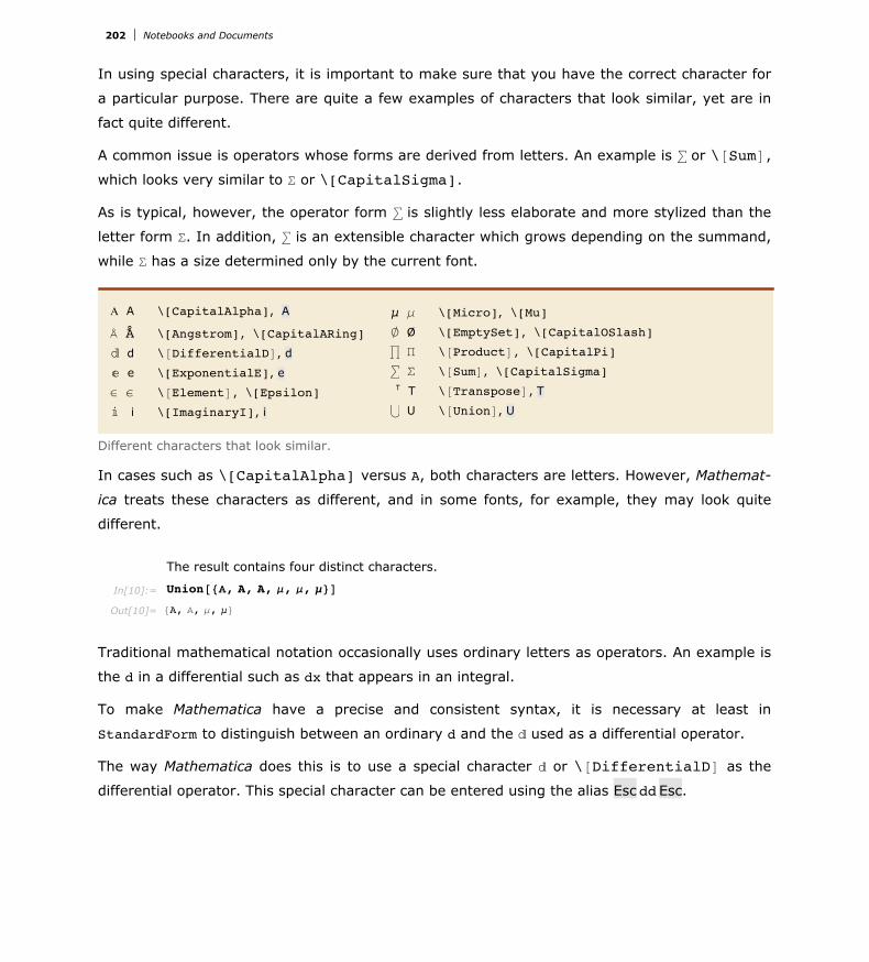
In using special characters, it is important to make sure that you have the correct character for

a particular purpose. There are quite a few examples of characters that look similar, yet are in

fact quite different.

A common issue is operators whose forms are derived from letters. An example is ⁄ or \@SumD,

which looks very similar to S or \[CapitalSigma].

As is typical, however, the operator form ⁄ is slightly less elaborate and more stylized than the

letter form S. In addition, ⁄ is an extensible character which grows depending on the summand,

while S has a size determined only by the current font.

A A \[CapitalAlpha], A

fi Å \[Angstrom], \[CapitalARing]

„ d \@DifferentialDD, d

‰ e \[ExponentialE], e

œ e \@ElementD , \[Epsilon]

Â i \[ImaginaryI], i

µ m \[Micro], \[Mu]

« Ø \[EmptySet], \[CapitalOSlash]

¤ P \@ProductD , \[CapitalPi]

⁄ S \@SumD, \[CapitalSigma]

T \@TransposeD, T

‹ U \@UnionD, U

Different characters that look similar.

In cases such as \[CapitalAlpha] versus A, both characters are letters. However, Mathemat-

ica treats these characters as different, and in some fonts, for example, they may look quite

different.

The result contains four distinct characters.

In[10]:= Union@8A, A, A, m, m, µ<D

Out[10]= 8A, A, m, µ<

Traditional mathematical notation occasionally uses ordinary letters as operators. An example is

the d in a differential such as dx that appears in an integral.

To make Mathematica have a precise and consistent syntax, it is necessary at least in

StandardForm to distinguish between an ordinary d and the „ used as a differential operator.

The way Mathematica does this is to use a special character „ or \@DifferentialDD as the

differential operator. This special character can be entered using the alias Esc ddEsc.


Mathematica uses a special character for the differential operator, so there is no conflict with an ordinary d.

In[11]:= ‡ xd „x

Out[11]=x1+d

1 + d

When letters and letter-like forms appear in Mathematica input, they are typically treated as

names of symbols. But when operators appear, functions must be constructed that correspond

to these operators. In almost all cases, what Mathematica does is to create a function whose

name is the full name of the special character that appears as the operator.

Mathematica constructs a CirclePlus function to correspond to the operator ⊕, whose full name is î[CirclePlus].

In[12]:= a ⊕ b ⊕ c êê FullForm

Out[12]//FullForm= CirclePlus@a, b, cD

This constructs an And function, which happens to have built-in evaluation rules in Mathematica.

In[13]:= a Ï b Ï c êê FullForm

Out[13]//FullForm= And@a, b, cD

Following the correspondence between operator names and function names, special characters

such as ‹ that represent built-in Mathematica functions have names that correspond to those

functions. Thus, for example, ¸ is named \@DivideD to correspond to the built-in Mathematica

function Divide, and fl is named \@ImpliesD to correspond to the built-in function Implies.

In general, however, special characters in Mathematica are given names that are as generic as

possible, so as not to prejudice different uses. Most often, characters are thus named mainly

according to their appearance. The character ⊕ is therefore named \@CirclePlusD, rather

than, say \@DirectSumD, and º is named \@TildeTildeD rather than, say,

\@ApproximatelyEqualD.


µ ä \@TimesD, \@CrossD

fl Ô \@AndD, \@WedgeD

fi Ó \@OrD, \@VeeD

Ø Ø \@RuleD, \@RightArrowD

fl fl \@ImpliesD , \@DoubleRightArrowD

= \@LongEqualD, =

\@PiecewiseD,

* * \@StarD, *

î \ \@BackslashD, \

ÿ . \@CenterDotD, .

Ô ^ \@WedgeD, ^

˝ | \@VerticalBarD, |

» | \@VerticalSeparatorD, |

X < \@LeftAngleBracketD , <

Different operator characters that look similar.

There are sometimes characters that look similar but which are used to represent different

operators. An example is \@TimesD and \@CrossD. \@TimesD corresponds to the ordinary

Times function for multiplication; \@CrossD corresponds to the Cross function for vector cross

products. The ä for \@CrossD is drawn slightly smaller than µ for \@TimesD, corresponding to

usual careful usage in mathematical typography.

The \@TimesD operator represents ordinary multiplication.

In[14]:= 85, 6, 7< µ 82, 3, 1<

Out[14]= 810, 18, 7<

The \@CrossD operator represents vector cross products.

In[15]:= 85, 6, 7< ä 82, 3, 1<

Out[15]= 8-15, 9, 3<

The two operators display in a similar way~with \@TimesD slightly larger than \@CrossD.

In[16]:= 8a µ b, a ä b<

Out[16]= 8a b, aäb<

In the example of \@AndD and \@WedgeD, the \@AndD operator~which happens to be drawn

slightly larger~corresponds to the built-in Mathematica function And, while the \@WedgeD

operator has a generic name based on the appearance of the character and has no built-in

meaning.


You can mix î[Wedge] and î[And] operators. Each has a definite precedence.

In[17]:= a Ô b Ï c Ô d êê FullForm

Out[17]//FullForm= And@Wedge@a, bD, Wedge@c, dDD

Some of the special characters commonly used as operators in mathematical notation look

similar to ordinary keyboard characters. Thus, for example, Ô or î[Wedge] looks similar to the ^

character on a standard keyboard.

Mathematica interprets a raw ^ as a power. But it interprets Ô as a generic Wedge function. In

cases such as this where there is a special character that looks similar to an ordinary keyboard

character, the convention is to use the ordinary keyboard character as the alias for the special

character. Thus, for example, Esc Êsc is the alias for \@WedgeD.

The raw ^ is interpreted as a power, but the Esc Êsc is a generic wedge operator.

In[18]:= x ^ y, x Esc Êsc y

Out[18]= 9xy, xÔy=

A related convention is that when a special character is used to represent an operator that can

be typed using ordinary keyboard characters, those characters are used in the alias for the

special character. Thus, for example, Esc ->Esc is the alias for Ø or \@RuleD, while Esc &&Esc

is the alias for fl or \@AndD.

Esc ->Esc is the alias for \@RuleD, and Esc &&Esc for \@AndD.

In[19]:= x Esc ->Esc y, x Esc &&Esc y // FullFormOut[19]//FullForm= List@Rule@x, yD, And@x, yDD

The most extreme case of characters that look alike but work differently occurs with vertical

bars.

form character name alias interpretationx y Alternatives@x,yDx y \@VerticalSeparatorD Esc Esc VerticalSeparator@x,yDx˝y \@VerticalBarD Esc â Esc VerticalBar@x,yD†x§ \@LeftBracketingBarD Esc l Esc BracketingBar@xD

\@RightBracketingBarD Esc r Esc

Different types of vertical bars.


Notice that the alias for \@VerticalBarD is Esc â|Esc, while the alias for the somewhat more

common \@VerticalSeparatorD is Esc |Esc. Mathematica often gives similar-looking charac-

ters similar aliases; it is a general convention that the aliases for the less commonly used

characters are distinguished by having spaces at the beginning.

Esc nnnEsc built-in alias for a common character

Esc â nnn Esc built-in alias for similar but less common character

Esc .nnnEsc alias globally defined in a Mathematica session

Esc ,nnnEsc alias defined in a specific notebook

Conventions for special character aliases.

The notebook front end for Mathematica often allows you to set up your own aliases for special

characters. If you want to, you can overwrite the built-in aliases. But the convention is to use

aliases that begin with a dot or comma.

Note that whatever aliases you may use to enter special characters, the full names of the

characters will always be used when the characters are stored in files.

Names of Symbols and Mathematical Objects

Mathematica by default interprets any sequence of letters or letter-like forms as the name of a

symbol.

All these are treated by Mathematica as symbols.

In[1]:= 8x, Sa, R¶, , ¡, —ABC, ‡X, m…n<

Out[1]= 8x, Sa, R¶, , ¡, —ABC, ‡X, m…n<

form character name alias interpretationp \[Pi] Esc pEsc, Esc piEsc equivalent to Pi¶ \[Infinity] Esc infEsc equivalent to Infinity‰ \[ExponentialE] Esc eeEsc equivalent to EÂ \[ImaginaryI] Esc iiEsc equivalent to I¸ \[ImaginaryJ] Esc jjEsc equivalent to I

Symbols with built-in meanings whose names do not start with capital English letters.


Essentially all symbols with built-in meanings in Mathematica have names that start with capital

English letters. Among the exceptions are ‰ and Â, which correspond to E and I respectively.

Forms such as ‰ are used for both input and output in StandardForm.

In[2]:= 8‰^H2 p ÂL, ‰^p<

Out[2]= 91, ‰p=

In OutputForm ‰ is output as E.

In[3]:= OutputForm@%D

Out[3]//OutputForm= Pi1, E

In written material, it is standard to use very short names~often single letters~for most of the

mathematical objects that one considers. But in Mathematica, it is usually better to use longer

and more explicit names.

In written material you can always explain that a particular single-letter name means one thing

in one place and another in another place. But in Mathematica, unless you use different con-

texts, a global symbol with a particular name will always be assumed to mean the same thing.

As a result, it is typically better to use longer names, which are more likely to be unique, and

which describe more explicitly what they mean.

For variables to which no value will be assigned, or for local symbols, it is nevertheless conve-

nient and appropriate to use short, often single-letter, names.

It is sensible to give the global function LagrangianL a long and explicit name. The local variables can be given short names.

In[4]:= LagrangianL@f_, m_D = HÑfL2 + m2 f2

Out[4]= m2 f2 + HÑfL2


form input interpretationxn x Ctrl+_ n Ctrl+Space Subscript@x,nDx+ x Ctrl+_ + Ctrl+Space SubPlus@xDx- x Ctrl+_ - Ctrl+Space SubMinus@xDx* x Ctrl+_ * Ctrl+Space SubStar@xDx+ x Ctrl+^ + Ctrl+Space SuperPlus@xDx- x Ctrl+^ - Ctrl+Space SuperMinus@xDx* x Ctrl+^ * Ctrl+Space SuperStar@xDx† x Ctrl+^ Esc dgEsc Ctrl+Space SuperDagger@xDx x Ctrl+& _ Ctrl+Space OverBar@xDx” x Ctrl+& Esc vecEsc Ctrl+Space OverVector@xDxè x Ctrl+& ~ Ctrl+Space OverTilde@xDx` x Ctrl+& ^ Ctrl+Space OverHat@xDx° x Ctrl+& . Ctrl+Space OverDot@xDx x Ctrl++ _ Ctrl+Space UnderBar@xDx StyleAx,BoldE x

Creating objects with annotated names.

Note that with a notebook front end, you can change the style of text using menu items.


SingleLetterItalics False whether to use italics for single-letter symbol names

MultiLetterItalics False whether to use italics for multi-letter symbol names

SingleLetterStyle None the style name or directives to use for single-letter symbol names

MultiLetterStyle None the style name or directives to use for multi-letter symbol names

Options for cells in a notebook.

It is conventional in traditional mathematical notation that names consisting of single ordinary

English letters are normally shown in italics, while other names are not. If you use

TraditionalForm, then Mathematica will by default follow this convention. You can explicitly

specify whether you want the convention followed by setting the SingleLetterItalics option

for particular cells or cell styles. You can further specify styles for names using single English

letters or multiple English letters by specifying values for the options SingleLetterStyle and

MultiLetterStyle.


Letters and Letter-like Forms

Greek Letters

form full name aliasesa \[Alpha] ÇaÇ, ÇalphaÇ

b \[Beta] ÇbÇ, ÇbetaÇ

g \[Gamma] ÇgÇ, ÇgammaÇ

d \[Delta] ÇdÇ, ÇdeltaÇ

e \[Epsilon] ÇeÇ, ÇepsilonÇ

ε \[CurlyEpsilon] ÇceÇ, ÇcepsilonÇ

z \[Zeta] ÇzÇ, ÇzetaÇ

h \[Eta] ÇhÇ, ÇetÇ, ÇetaÇ

q \[Theta] ÇqÇ, ÇthÇ, ÇthetaÇ

J \[CurlyTheta] ÇcqÇ, ÇcthÇ, ÇcthetaÇ

i \[Iota] ÇiÇ, ÇiotaÇ

k \[Kappa] ÇkÇ, ÇkappaÇ

ø \[CurlyKappa] ÇckÇ, ÇckappaÇ

l \[Lambda] ÇlÇ, ÇlambdaÇ

m \[Mu] ÇmÇ, ÇmuÇ

n \[Nu] ÇnÇ, ÇnuÇ

x \[Xi] ÇxÇ, ÇxiÇ

o \[Omicron] ÇomÇ, ÇomicronÇ

p \[Pi] ÇpÇ, ÇpiÇ

v \[CurlyPi] ÇcpÇ, ÇcpiÇ

r \[Rho] ÇrÇ, ÇrhoÇ

ϱ \[CurlyRho] ÇcrÇ, ÇcrhoÇ

s \[Sigma] ÇsÇ, ÇsigmaÇ

V \[FinalSigma] ÇfsÇ

t \[Tau] ÇtÇ, ÇtauÇ

u \[Upsilon] ÇuÇ, ÇupsilonÇ

form full name aliasesA \[CapitalAlpha] ÇAÇ, ÇAlphaÇ

B \[CapitalBeta] ÇBÇ, ÇBetaÇ

G \[CapitalGamma] ÇGÇ, ÇGammaÇ

D \[CapitalDelta] ÇDÇ, ÇDeltaÇ

E \[CapitalEpsilon] ÇEÇ, ÇEpsilonÇ

Z \[CapitalZeta] ÇZÇ, ÇZetaÇ

H \[CapitalEta] ÇHÇ, ÇEtÇ, ÇEtaÇ

Q \[CapitalTheta] ÇQÇ, ÇThÇ, ÇThetaÇ

I \[CapitalIota] ÇIÇ, ÇIotaÇ

K \[CapitalKappa] ÇKÇ, ÇKappaÇ

L \[CapitalLambda] ÇLÇ, ÇLambdaÇ

M \[CapitalMu] ÇMÇ, ÇMuÇ

N \[CapitalNu] ÇNÇ, ÇNuÇ

X \[CapitalXi] ÇXÇ, ÇXiÇ

O \[CapitalOmicron] ÇOmÇ, ÇOmicronÇ

P \[CapitalPi] ÇPÇ, ÇPiÇ

R \[CapitalRho] ÇRÇ, ÇRhoÇ

S \[CapitalSigma] ÇSÇ, ÇSigmaÇ

T \[CapitalTau] ÇTÇ, ÇTauÇ

U \[CapitalUpsilon] ÇUÇ, ÇUpsilonÇ

¢ \[CurlyCapitalUpsilon] ÇcUÇ, ÇcUpsilonÇ


form full name aliasesf \[Phi] ÇfÇ, ÇphÇ, ÇphiÇ

j \[CurlyPhi] ÇjÇ, ÇcphÇ, ÇcphiÇ

c \[Chi] ÇcÇ, ÇchÇ, ÇchiÇ

y \[Psi] ÇyÇ, ÇpsÇ, ÇpsiÇ

w \[Omega] ÇoÇ, ÇwÇ, ÇomegaÇ

ϝ \[Digamma] ÇdiÇ, ÇdigammaÇ

ϟ \[Koppa] ÇkoÇ, ÇkoppaÇ

ϛ \[Stigma] ÇstiÇ, ÇstigmaÇ

ª \[Sampi] ÇsaÇ, ÇsampiÇ

form full name aliases¢ \[CurlyCapitalUpsilon] ÇcUÇ, ÇcUpsilonÇ

F \[CapitalPhi] ÇFÇ, ÇPhÇ, ÇPhiÇ

C \[CapitalChi] ÇCÇ, ÇChÇ, ÇChiÇ

Y \[CapitalPsi] ÇYÇ, ÇPsÇ, ÇPsiÇ

W \[CapitalOmega] ÇOÇ, ÇWÇ, ÇOmegaÇ

Ϝ \[CapitalDigamma] ÇDiÇ, ÇDigammaÇ

¥ \[CapitalKoppa] ÇKoÇ, ÇKoppaÇ

Ϛ \[CapitalStigma] ÇStiÇ, ÇStigmaÇ

µ \[CapitalSampi] ÇSaÇ, ÇSampiÇ

The complete collection of Greek letters in Mathematica.

You can use Greek letters as the names of symbols. The only Greek letter with a built-in mean-

ing in StandardForm is p, which Mathematica takes to stand for the symbol Pi.

Note that even though p on its own is assigned a built-in meaning, combinations such as p2 or

xp have no built-in meanings.

The Greek letters S and P look very much like the operators for sum and product. But as dis-

cussed above, these operators are different characters, entered as î[Sum] and î[Product] respec -

tively.

Similarly, e is different from the œ operator î[Element], and m is different from µ or î[Micro].

Some capital Greek letters such as î[CapitalAlpha] look essentially the same as capital English

letters. Mathematica however treats them as different characters, and in TraditionalForm it

uses î[CapitalBeta], for example, to denote the built-in function Beta.

Following common convention, lower-case Greek letters are rendered slightly slanted in the

standard fonts provided with Mathematica, while capital Greek letters are unslanted. On Greek

systems, however, Mathematica will render all Greek letters unslanted so that standard Greek

fonts can be used.

Almost all Greek letters that do not look similar to English letters are widely used in science and

mathematics. The capital xi X is rare, though it is used to denote the cascade hyperon particles,

the grand canonical partition function and regular language complexity. The capital upsilon U is

also rare, though it is used to denote b b particles, as well as the vernal equinox.

Curly Greek letters are often assumed to have different meanings from their ordinary counter-

parts. Indeed, in pure mathematics a single formula can sometimes contain both curly and

ordinary forms of a particular letter. The curly pi v is rare, except in astronomy.


Curly Greek letters are often assumed to have different meanings from their ordinary counter-

parts. Indeed, in pure mathematics a single formula can sometimes contain both curly and

ordinary forms of a particular letter. The curly pi v is rare, except in astronomy.

The final sigma V is used for sigmas that appear at the ends of words in written Greek; it is not

commonly used in technical notation.

The digamma ϝ, koppa ϟ, stigma ϛ and sampi ª are archaic Greek letters. These letters provide

a convenient extension to the usual set of Greek letters. They are sometimes needed in making

correspondences with English letters. The digamma corresponds to an English w, and koppa to

an English q. Digamma is occasionally used to denote the digamma function PolyGamma@xD.

Variants of English Letters

form full name alias \[ScriptL] ÇsclÇ

\[ScriptCapitalE] ÇscEÇ

\[ScriptCapitalH] ÇscHÇ

\[ScriptCapitalL] ÇscLÇ

ℭ \[GothicCapitalC] ÇgoCÇ

ℌ \[GothicCapitalH] ÇgoHÇ

¬ \[GothicCapitalI] ÇgoIÇ

ℜ \[GothicCapitalR] ÇgoRÇ

form full name alias \[DoubleStruckCapitalC] ÇdsCÇ

\[DoubleStruckCapitalR] ÇdsRÇ

\[DoubleStruckCapitalQ] ÇdsQÇ

\[DoubleStruckCapitalZ] ÇdsZÇ

\[DoubleStruckCapitalN] ÇdsNÇ

“ \[DotlessI]‘ \[DotlessJ]ƒ \[WeierstrassP] ÇwpÇ

Some commonly used variants of English letters.

By using menu items in the notebook front end, you can make changes in the font and style of

ordinary text. However, such changes are usually discarded whenever you send input to the

Mathematica kernel.

Script, gothic and double-struck characters are, however, treated as fundamentally different

from their ordinary forms. This means that even though a C that is italic or a different size will

be considered equivalent to an ordinary C when fed to the kernel, a double-struck will not.

Different styles and sizes of C are treated as the same by the kernel. But gothic and double-struck characters are treated as different.

In[9]:= C + C +C + ℭ +

Out[9]= 3 C + ℭ +

In standard mathematical notation, capital script and gothic letters are sometimes used inter-

changeably. The double-struck letters, sometimes called blackboard or openface letters, are

conventionally used to denote specific sets. Thus, for example, conventionally denotes the set

of complex numbers, and the set of integers.


In standard mathematical notation, capital script and gothic letters are sometimes used inter-

changeably. The double-struck letters, sometimes called blackboard or openface letters, are

conventionally used to denote specific sets. Thus, for example, conventionally denotes the set

of complex numbers, and the set of integers.

Dotless i and j are not usually taken to be different in meaning from ordinary i and j; they are

simply used when overscripts are being placed on the ordinary characters.

î[WeierstrassP] is a notation specifically used for the Weierstrass P function WeierstrassP.

full names aliases\[ScriptA] | \[ScriptZ] ÇscaÇ | ÇsczÇ lowercase script letters\[ScriptCapitalA] | \[ScriptCapitalZ]

ÇscAÇ | ÇscZÇ uppercase script letters\[GothicA] | \[GothicZ] ÇgoaÇ | ÇgozÇ lowercase gothic letters\[GothicCapitalA] | \[GothicCapitalZ]

ÇgoAÇ | ÇgoZÇ uppercase gothic letters\[DoubleStruckA] | \[DoubleStruckZ]

ÇdsaÇ | ÇdszÇ lowercase double-struck letters

\[DoubleStruckCapitalA] | \[DoubleStruckCapitalZ]ÇdsAÇ | ÇdsZÇ uppercase double-struck

letters\[FormalA] | \[FormalZ]

Ç$aÇ | Ç$zÇ lowercase formal letters\[FormalCapitalA] | \[FormalCapitalZ]

Ç$AÇ | Ç$ZÇ uppercase formal letters

Complete alphabets of variant English letters.

Formal Symbols

Symbols represented by formal letters, or formal symbols, appear in the output of certain

functions. They are indicated by gray dots above and below the English letter.

DifferentialRoot automatically chooses the names for the function arguments.

In[83]:= root = DifferentialRootReduce@CosD

Out[83]= DifferentialRootAFunctionA9y.., x

.

.=, 9y..Ax

.

.E + y..££Ax..E ã 0, y

.

.@0D ã 1, y..£@0D ã 0=EE


Formal symbols are Protected, so they cannot be accidentally assigned a value.

Trying to modify a formal symbol fails.

In[2]:= y.. = 0

Set::wrsym: Symbol y.. is Protected. à

Out[2]= 0

In[3]:= y..

Out[3]= y..

This means that expressions depending on formal symbols will not be accidentally modified.

In[4]:= root@@1, 2DD

Out[4]= 9y..Ax..E + y

.

.££Ax..E ã 0, y

.

.@0D ã 1, y..£@0D ã 0=

Specific values for formal symbols can be substituted using replacement rules.

Verify that the defining equations hold for cosine.

In[5]:= root@@1, 2DD ê. y.. Ø Cos

Out[5]= 8True, True, True<

Formal symbols can be temporarily modified inside of a Block because Block clears all defini-

tions associated with a symbol, including Attributes. Table works essentially like Block, thus

also allowing temporary changes.

Assign a temporary value to y..:

In[6]:= BlockA9y.. = Cos=, root@@1, 2DDE

Out[6]= 8True, True, True<

In most situations modifying formal symbols is not necessary. Since in DifferentialRoot

formal symbols are used as names for the formal parameters of a function, the function should

simply be evaluated for the actual values of arguments.

Evaluating the function substitutes x for x.. and y for y

.

..

In[7]:= root@@1DD@y, xD

Out[7]= 8y@xD + y££@xD ã 0, y@0D ã 1, y£@0D ã 0<


It is possible to define custom typesetting rules for formal symbols.

Use coloring to highlight formal symbols.

In[84]:= MakeBoxesAx.., _E := TagBoxA"x", x

.

. &, AutoDelete Ø True,BaseStyle Ø 8FontColor Ø [email protected], .4, .2D, ShowSyntaxStyles Ø False<E

MakeBoxesAy.., _E := TagBoxA"y", y

.

. &, AutoDelete Ø True,

BaseStyle Ø 8FontColor Ø [email protected], .4, .2D, ShowSyntaxStyles Ø False<E

In[86]:= root

Out[86]=

The formatting rules were attached to MakeBoxes. Restore the original formatting:

In[87]:= FormatValuesüMakeBoxes = 8<;

In[88]:= root

Out[88]= DifferentialRootAFunctionA9y.., x

.

.=, 9y..Ax

.

.E + y..££Ax..E ã 0, y

.

.@0D ã 1, y..£@0D ã 0=EE

Hebrew Letters

form full name alias¡ \[Aleph] ÇalÇ

º \[Bet]

form full nameℷ \[Gimel]æ \[Dalet]

Hebrew characters.

Hebrew characters are used in mathematics in the theory of transfinite sets; ¡0 is for example

used to denote the total number of integers.


Units and Letter-Like Mathematical Symbols

form full name aliasµ \[Micro] ÇmiÇ

\[Mho] ÇmhoÇ

fi \[Angstrom] ÇAngÇ

— \[HBar] ÇhbÇ

¢ \[Cent] ÇcentÇ

£ \[Sterling] \[Euro] ÇeuroÇ

¥ \[Yen]

form full name alias° \[Degree] ÇdegÇ

« \[EmptySet] ÇesÇ

¶ \[Infinity] ÇinfÇ

‰ \[ExponentialE] ÇeeÇ

Â \[ImaginaryI] ÇiiÇ

¸ \[ImaginaryJ] ÇjjÇ

˛ \[DoubledPi] ÇppÇ

˝ \[DoubledGamma] ÇggÇ

Units and letter-like mathematical symbols.

Mathematica treats ° or \[Degree] as the symbol Degree, so that, for example, 30 ° is equiva-

lent to 30 Degree.

Note that µ, fi and « are all distinct from the ordinary letters m (\[Mu]), Å

(\[CapitalARing]) and Ø (\[CapitalOSlash]).

Mathematica interprets ¶ as Infinity, ‰ as E, and both Â and ¸ as I. The characters ‰, Â and ¸

are provided as alternatives to the usual uppercase letters E and I.

˛ and ˝ are not by default assigned meanings in StandardForm. You can therefore use ˛ to

represent a pi that will not automatically be treated as Pi. In TraditionalForm ˝ is interpreted

as EulerGamma.

form full name alias∂ \@PartialDD ÇpdÇ

„ \@DifferentialDD ÇddÇ

ˇ \@CapitalDifferentialDD ÇDDÇ

“ \@DelD ÇdelÇ

\@DifferenceDeltaD ÇdiffdÇ

form full name alias

‚ \@SumD ÇsumÇ

‰ \@ProductD ÇprodÇ

\@TransposeD ÇtrÇ

\@HermitianConjugateD ÇhcÇ

\@DiscreteShiftD ÇshiftÇ

\@DiscreteRatioD ÇdratioÇ

Operators that look like letters.


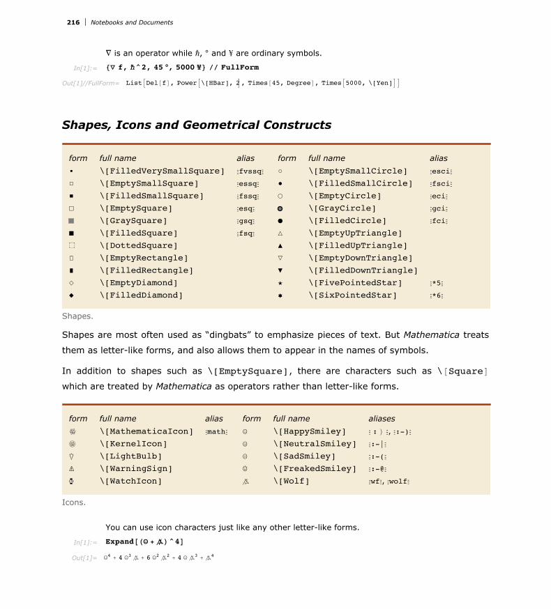
“ is an operator while —, ° and ¥ are ordinary symbols.

In[1]:= 8“ f, —^2, 45 °, 5000 ¥< êê FullForm

Out[1]//FullForm= ListADel@fD, PowerA\[HBar], 2E, Times@45, DegreeD, TimesA5000, \[Yen]EE

Shapes, Icons and Geometrical Constructs

form full name alias‰ \[FilledVerySmallSquare] ÇfvssqÇ

„ \[EmptySmallSquare] ÇessqÇ

† \[FilledSmallSquare] ÇfssqÇ

· \[EmptySquare] ÇesqÇ

\[GraySquare] ÇgsqÇ

‡ \[FilledSquare] ÇfsqÇ

Ó \[DottedSquare]Ò \[EmptyRectangle] \[FilledRectangle]Ì \[EmptyDiamond]Ï \[FilledDiamond]

form full name aliasÈ \[EmptySmallCircle] ÇesciÇ

Ë \[FilledSmallCircle] ÇfsciÇ

Á \[EmptyCircle] ÇeciÇ

\[GrayCircle] ÇgciÇ

Ê \[FilledCircle] ÇfciÇ

Û \[EmptyUpTriangle]Ú \[FilledUpTriangle]ı \[EmptyDownTriangle]Ù \[FilledDownTriangle]¯ \[FivePointedStar] Ç*5Ç

˜ \[SixPointedStar] Ç*6Ç

Shapes.

Shapes are most often used as “dingbats” to emphasize pieces of text. But Mathematica treats

them as letter-like forms, and also allows them to appear in the names of symbols.

In addition to shapes such as \[EmptySquare], there are characters such as \@SquareD

which are treated by Mathematica as operators rather than letter-like forms.

form full name aliasŸ \[MathematicaIcon] ÇmathÇ

⁄ \[KernelIcon]¤ \[LightBulb]‹ \[WarningSign]› \[WatchIcon]

form full name aliasesÃ \[HappySmiley] Ç : L Ç, Ç:-)Ç

Õ \[NeutralSmiley] Ç:-|Ç

Œ \[SadSmiley] Ç:-(Ç

œ \[FreakedSmiley] Ç:-@Ç

\[Wolf] ÇwfÇ, ÇwolfÇ

Icons.

You can use icon characters just like any other letter-like forms.

In[1]:= Expand@HÃ +L^4D

Out[1]= Ã4 + 4 Ã

3 + 6 Ã2 2 + 4 Ã 3 + 4


form full name— \[Angle]¨ \[RightAngle]∡ \[MeasuredAngle]

form full nameÆ \[SphericalAngle]Û \[EmptyUpTriangle]Ø \[Diameter]

Notation for geometrical constructs.

Since Mathematica treats characters like — as letter-like forms, constructs like —BC are treated in

Mathematica as single symbols.

Textual Elements

form full name alias| \[Dash] Ç-Ç

~ \[LongDash] Ç--Ç

• \[Bullet] ÇbuÇ

¶ \[Paragraph]§ \[Section]¿ \[DownQuestion] Çd?Ç

¡ \[DownExclamation] Çd!Ç

form full name alias£ \[Prime] Ç'Ç

″ \[DoublePrime] Ç''Ç

æ \[ReversePrime] Ç`Ç

ø \[ReverseDoublePrime] Ç``Ç

« \[LeftGuillemet] Çg<<Ç

» \[RightGuillemet] Çg>>Ç

… \[Ellipsis] Ç...Ç

Characters used for punctuation and annotation.

form full name© \[Copyright]® \[RegisteredTrademark]’ \[Trademark]Ÿ \[Flat]⁄ \[Natural]¤ \[Sharp]

form full name alias† \[Dagger] ÇdgÇ

‡ \[DoubleDagger] ÇddgÇ

® \[ClubSuit]© \[DiamondSuit]™ \[HeartSuit]´ \[SpadeSuit]

Other characters used in text.


form full name alias\[HorizontalLine] ÇhlineÇ

\[VerticalLine] ÇvlineÇ

… \[Ellipsis] Ç...Ç

\[CenterEllipsis]ª \[VerticalEllipsis]⋰ \[AscendingEllipsis] \[DescendingEllipsis]

form full name alias† \[UnderParenthesis] Çu(Ç

ê \[OverParenthesis] Ço(Ç

Ä \[UnderBracket] Çu[Ç

p \[OverBracket] Ço[Ç

ß \[UnderBrace] ÇuÇ

ó \[OverBrace] ÇoÇ

Characters used in building sequences and arrays.

The under and over braces grow to enclose the whole expression.

In[1]:= Underoverscript@Expand@H1 + xL^4D, ß, óD

Out[1]= 1 + 4 x + 6 x2 + 4 x3 + x4

Extended Latin Letters

Mathematica supports all the characters commonly used in Western European languages based

on Latin scripts.

form full name aliasà \[AGrave] Ça`Ç

á \[AAcute] Ça'Ç

â \[AHat] Ça^Ç

ã \[ATilde] Ça~Ç

ä \[ADoubleDot] Ça"Ç

å \[ARing] ÇaoÇ

ā \[ABar] Ça-Ç

ă \[ACup] ÇauÇ

æ \[AE] ÇaeÇ

ć \[CAcute] Çc'Ç

ç \[CCedilla] Çc,Ç

č \[CHacek] ÇcvÇ

è \[EGrave] Çe`Ç

é \[EAcute] Çe'Ç

ē \[EBar] Çe-Ç

ê \[EHat] Çe^Ç

ë \[EDoubleDot] Çe"Ç

ĕ \[ECup] ÇeuÇ

ì \[IGrave] Çi`Ç

í \[IAcute] Çi'Ç

î \[IHat] Çi^Ç

ï \[IDoubleDot] Çi"Ç

ĭ \[ICup] ÇiuÇ

ð \[Eth] Çd-Ç

ł \[LSlash] Çl/Ç

ñ \[NTilde] Çn~Ç

ò \[OGrave] Ço`Ç

ó \[OAcute] Ço'Ç

ô \[OHat] Ço^Ç

õ \[OTilde] Ço~Ç

ö \[ODoubleDot] Ço"Ç

ő \[ODoubleAcute] Ço''Ç

ø \[OSlash] Ço/Ç

œ \[OE] ÇoeÇ

š \[SHacek] ÇsvÇ

ù \[UGrave] Çu`Ç

ú \[UAcute] Çu'Ç

û \[UHat] Çu^Ç

ü \[UDoubleDot] Çu"Ç

ű \[UDoubleAcute] Çu''Ç

ý \[YAcute] Çy'Ç

þ \[Thorn] ÇthnÇ

ß \[SZ] ÇszÇ, ÇssÇ

form full name aliasÀ \[CapitalAGrave] ÇA`Ç

Á \[CapitalAAcute] ÇA'Ç

Â \[CapitalAHat] ÇA^Ç

Ã \[CapitalATilde] ÇA~Ç

Ä \[CapitalADoubleDot] ÇA"Ç

Å \[CapitalARing] ÇAoÇ

Ā \[CapitalABar] ÇA-Ç

Ă \[CapitalACup] ÇAuÇ

Æ \[CapitalAE] ÇAEÇ

Ć \[CapitalCAcute] ÇC'Ç

Ç \[CapitalCCedilla] ÇC,Ç

Č \[CapitalCHacek] ÇCvÇ

È \[CapitalEGrave] ÇE`Ç

É \[CapitalEAcute] ÇE'Ç

Ē \[CapitalEBar] ÇE-Ç

Ê \[CapitalEHat] ÇE^Ç

Ë \[CapitalEDoubleDot] ÇE"Ç

Ĕ \[CapitalECup] ÇEuÇ

Ì \[CapitalIGrave] ÇI`Ç

Í \[CapitalIAcute] ÇI'Ç

Î \[CapitalIHat] ÇI^Ç

Ï \[CapitalIDoubleDot] ÇI"Ç

Ĭ \[CapitalICup] ÇIuÇ

Ð \[CapitalEth] ÇD-Ç

Ł \[CapitalLSlash] ÇL/Ç

Ñ \[CapitalNTilde] ÇN~Ç

Ò \[CapitalOGrave] ÇO`Ç

Ó \[CapitalOAcute] ÇO'Ç

Ô \[CapitalOHat] ÇO^Ç

Õ \[CapitalOTilde] ÇO~Ç

Ö \[CapitalODoubleDot] ÇO"Ç

Ő \[CapitalODoubleAcute] ÇO''Ç

Ø \[CapitalOSlash] ÇO/Ç

Œ \[CapitalOE] ÇOEÇ

Š \[CapitalSHacek] ÇSvÇ

Ù \[CapitalUGrave] ÇU`Ç

Ú \[CapitalUAcute] ÇU'Ç

Û \[CapitalUHat] ÇU^Ç

Ü \[CapitalUDoubleDot] ÇU"Ç

Ű \[CapitalUDoubleAcute] ÇU''Ç

Ý \[CapitalYAcute] ÇY'Ç

Þ \[CapitalThorn] ÇThnÇ


form full name aliasà \[AGrave] Ça`Ç

á \[AAcute] Ça'Ç

â \[AHat] Ça^Ç

ã \[ATilde] Ça~Ç

ä \[ADoubleDot] Ça"Ç

å \[ARing] ÇaoÇ

ā \[ABar] Ça-Ç

ă \[ACup] ÇauÇ

æ \[AE] ÇaeÇ

ć \[CAcute] Çc'Ç

ç \[CCedilla] Çc,Ç

č \[CHacek] ÇcvÇ

è \[EGrave] Çe`Ç

é \[EAcute] Çe'Ç

ē \[EBar] Çe-Ç

ê \[EHat] Çe^Ç

ĕ \[ECup] ÇeuÇ

ì \[IGrave] Çi`Ç

í \[IAcute] Çi'Ç

î \[IHat] Çi^Ç

ï \[IDoubleDot] Çi"Ç

ĭ \[ICup] ÇiuÇ

ð \[Eth] Çd-Ç

ł \[LSlash] Çl/Ç

ñ \[NTilde] Çn~Ç

ò \[OGrave] Ço`Ç

ó \[OAcute] Ço'Ç

ô \[OHat] Ço^Ç

õ \[OTilde] Ço~Ç

ö \[ODoubleDot] Ço"Ç

ő \[ODoubleAcute] Ço''Ç

ø \[OSlash] Ço/Ç

œ \[OE] ÇoeÇ

š \[SHacek] ÇsvÇ

ù \[UGrave] Çu`Ç

ú \[UAcute] Çu'Ç

û \[UHat] Çu^Ç

ü \[UDoubleDot] Çu"Ç

ű \[UDoubleAcute] Çu''Ç

ý \[YAcute] Çy'Ç

þ \[Thorn] ÇthnÇ

ß \[SZ] ÇszÇ, ÇssÇ

form full name aliasÀ \[CapitalAGrave] ÇA`Ç

Á \[CapitalAAcute] ÇA'Ç

Â \[CapitalAHat] ÇA^Ç

Ã \[CapitalATilde] ÇA~Ç

Ä \[CapitalADoubleDot] ÇA"Ç

Å \[CapitalARing] ÇAoÇ

Ā \[CapitalABar] ÇA-Ç

Ă \[CapitalACup] ÇAuÇ

Æ \[CapitalAE] ÇAEÇ

Ć \[CapitalCAcute] ÇC'Ç

Ç \[CapitalCCedilla] ÇC,Ç

Č \[CapitalCHacek] ÇCvÇ

È \[CapitalEGrave] ÇE`Ç

É \[CapitalEAcute] ÇE'Ç

Ē \[CapitalEBar] ÇE-Ç

Ê \[CapitalEHat] ÇE^Ç

Ĕ \[CapitalECup] ÇEuÇ

Ì \[CapitalIGrave] ÇI`Ç

Í \[CapitalIAcute] ÇI'Ç

Î \[CapitalIHat] ÇI^Ç

Ï \[CapitalIDoubleDot] ÇI"Ç

Ĭ \[CapitalICup] ÇIuÇ

Ð \[CapitalEth] ÇD-Ç

Ł \[CapitalLSlash] ÇL/Ç

Ñ \[CapitalNTilde] ÇN~Ç

Ò \[CapitalOGrave] ÇO`Ç

Ó \[CapitalOAcute] ÇO'Ç

Ô \[CapitalOHat] ÇO^Ç

Õ \[CapitalOTilde] ÇO~Ç

Ö \[CapitalODoubleDot] ÇO"Ç

Ő \[CapitalODoubleAcute] ÇO''Ç

Ø \[CapitalOSlash] ÇO/Ç

Œ \[CapitalOE] ÇOEÇ

Š \[CapitalSHacek] ÇSvÇ

Ù \[CapitalUGrave] ÇU`Ç

Ú \[CapitalUAcute] ÇU'Ç

Û \[CapitalUHat] ÇU^Ç

Ü \[CapitalUDoubleDot] ÇU"Ç

Ű \[CapitalUDoubleAcute] ÇU''Ç

Ý \[CapitalYAcute] ÇY'Ç

Þ \[CapitalThorn] ÇThnÇ

Variants of English letters.

Most of the characters shown are formed by adding diacritical marks to ordinary English letters.

Exceptions include \[SZ] ß, used in German, and \[Thorn] þ and \[Eth] ð, used primarily in

Old English.

You can make additional characters by explicitly adding diacritical marks yourself.

char Ctrl+& mark Ctrl+Space add a mark above a character

char Ctrl++ mark Ctrl+Space add a mark below a character

Adding marks above and below characters.


form alias full name' (keyboard character) \@RawQuoteD acute accent£ Ç' Ç \[Prime] acute accent` (keyboard character) \[RawBackquote] grave accentæ Ç`Ç \[ReversePrime] grave accent. . (keyboard characters) umlaut or diaeresis^ (keyboard character) \@RawWedgeD circumflex or hatÈ ÇesciÇ \[EmptySmallCirclÖ

e]ring

. (keyboard character) \@RawDotD dot~ (keyboard character) \@RawTildeD tilde_ (keyboard character) \[RawUnderscore] bar or macron« ÇhcÇ \[Hacek] hacek or checkÒ ÇbvÇ \[Breve] breveÚ ÇdbvÇ \[DownBreve] tie accent″ Ç'' Ç \[DoublePrime] long umlautfi ÇcdÇ \[Cedilla] cedilla

Diacritical marks to add to characters.

Operators

Basic Mathematical Operators

form full name aliasµ \@TimesD Ç*Ç

¸ \@DivideD ÇdivÇ

- \@SqrtD ÇsqrtÇ

form full name aliasä \@CrossD ÇcrossÇ

± \@PlusMinusD Ç+-Ç

° \@MinusPlusD Ç-+Ç

Some operators used in basic arithmetic and algebra.

Note that the ä for î[Cross] is distinguished by being drawn slightly smaller than the µ for î

[Times].


xµy Times@x,yD multiplicationx¸y Divide@x,yD division,x Sqrt@xD square rootxäy Cross@x,yD vector cross product±x PlusMinus@xD (no built-in meaning)x±y PlusMinus@x,yD (no built-in meaning)°x MinusPlus@xD (no built-in meaning)x°y MinusPlus@x,yD (no built-in meaning)

Interpretation of some operators in basic arithmetic and algebra.

Operators in Calculus and Algebra

form full name alias“ \@DelD ÇdelÇ

∂ \@PartialDD ÇpdÇ

„ \@DifferentialDD ÇddÇ

‚ \@SumD ÇsumÇ

‰ \@ProductD ÇprodÇ


Ÿ \@IntegralD ÇintÇ

ò \@ContourIntegralD ÇcintÇ

ô \@DoubleContourIntegralD

ö \@CounterClockwiseContourIntegralD ÇcccintÇ

õ \@ClockwiseContourIntegralD ÇccintÇ

Operators used in calculus.

form full name aliases \@ConjugateD ÇcoÇ, ÇconjÇ

\@TransposeD ÇtrÇ

form full name aliasæ \@ConjugateTransposeD ÇctÇ

\@HermitianConjugateD ÇhcÇ

Operators for complex numbers and matrices.


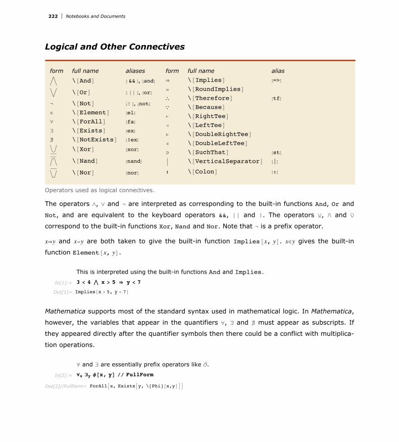
Logical and Other Connectives

form full name aliases

Ì \@AndD Ç && Ç, ÇandÇ

Î \@OrD Ç »» Ç, ÇorÇ

Ÿ \@NotD Ç! Ç, ÇnotÇ

œ \@ElementD ÇelÇ

" \@ForAllD ÇfaÇ

$ \@ExistsD ÇexÇ

± \@NotExistsD Ç!exÇ

\@XorD ÇxorÇ

\@NandD ÇnandÇ

\@NorD ÇnorÇ

form full name aliasfl \@ImpliesD Ç=>Ç

V \@RoundImpliesD\ \@ThereforeD ÇtfÇ

ã \@BecauseD¢ \@RightTeeD§ \@LeftTeeD£ \@DoubleRightTeeD• \@DoubleLeftTeeD' \@SuchThatD ÇstÇ

\@VerticalSeparatorD Ç|Ç

: \@ColonD Ç:Ç

Operators used as logical connectives.

The operators fl, fi and Ÿ are interpreted as corresponding to the built-in functions And, Or and

Not, and are equivalent to the keyboard operators &&, »» and !. The operators , and

correspond to the built-in functions Xor, Nand and Nor. Note that Ÿ is a prefix operator.

xfly and xVy are both taken to give the built-in function Implies@x, yD. xœy gives the built-in

function Element@x, yD.

This is interpreted using the built-in functions And and Implies.

In[1]:= 3 < 4 Ï x > 5 fl y < 7

Out[1]= Implies@x > 5, y < 7D

Mathematica supports most of the standard syntax used in mathematical logic. In Mathematica,

however, the variables that appear in the quantifiers ", $ and ± must appear as subscripts. If

they appeared directly after the quantifier symbols then there could be a conflict with multiplica-

tion operations.

" and $ are essentially prefix operators like ∂.

In[2]:= "x $y f@x, yD êê FullForm

Out[2]//FullForm= ForAllAx, ExistsAy, \[Phi]@x,yDEE

Operators Used to Represent Actions


Operators Used to Represent Actions

form full name aliasÎ \@SmallCircleD ÇscÇ

⊕ \@CirclePlusD Çc+Ç

û \@CircleMinusD Çc-Ç

⊗ \@CircleTimesD Çc*Ç

ü \@CircleDotD Çc.Ç

ù \@DiamondD ÇdiaÇ

ÿ \@CenterDotD Ç.Ç

* \@StarD ÇstarÇ

™ \@VerticalTildeDï \@BackslashD Ç\Ç

form full name aliasÔ \@WedgeD Ç^Ç

Ó \@VeeD ÇvÇ

Ê \@UnionD ÇunÇ

\@UnionPlusD

Ë \@IntersectionD ÇinterÇ

Æ \@SquareIntersectionD

Ø \@SquareUnionD

ˇ \@CoproductD ÇcoprodÇ

[ \@CapD\ \@CupDÑ \@SquareD ÇsqÇ

Operators typically used to represent actions. All the operators except î[Square] are infix.

Following Mathematica’s usual convention, all the operators in the table are interpreted to give

functions whose names are exactly the names of the characters that appear in the operators.

The operators are interpreted as functions with corresponding names.

In[3]:= x ⊕ y [ z êê FullForm

Out[3]//FullForm= CirclePlus@x, Cap@y, zDD

All the operators in the table above, except for Ñ, are infix, so that they must appear in

between their operands.


Bracketing Operators

form full name aliase \@LeftFloorD ÇlfÇ

u \@RightFloorD ÇrfÇ

a \@LeftCeilingD ÇlcÇ

q \@RightCeilingD ÇrcÇ

Q \@LeftDoubleBracketD Ç[[Ç

U \@RightDoubleBracketD Ç]]Ç

form full name aliasY \@LeftAngleBracketD Ç<Ç

] \@RightAngleBracketD Ç>Ç

° \@LeftBracketingBarD Çl|Ç

• \@RightBracketingBarD Çr|Ç

± \@LeftDoubleBracketingBarD Çl||Ç

µ \@RightDoubleBracketingBarD Çr||Ç

Characters used as bracketing operators.

dxt Floor@xD

`xp Ceiling@xD

mPi, j,…T Part@m,i, j,…D

Xx,y,…\ AngleBracket@x,y,…D

†x,y,…§ BracketingBar@x,y,…D

°x,y,…¥ DoubleBracketingBar@x,y,…D

Interpretations of bracketing operators.

Operators Used to Represent Relations

form full name aliasã \@EqualD Ç==Ç

\@LongEqualD Çl=Ç

ª \@CongruentD Ç===Ç

~ \@TildeD Ç~Ç

º \@TildeTildeD Ç~~Ç

> \@TildeEqualD Ç~=Ç

@ \@TildeFullEqualD Ç~==Ç

? \@EqualTildeD Ç=~Ç

P \@HumpEqualD Çh=Ç

Q \@HumpDownHumpD^ \@CupCapDU \@DotEqualD

form full name alias≠ \@NotEqualD Ç!=Ç

T \@NotCongruentD Ç!===Ç

L \@NotTildeD Ç!~Ç

M \@NotTildeTildeD Ç!~~Ç

N \@NotTildeEqualD Ç!~=Ç

= \@NotTildeFullEqualD Ç!~==Ç

O \@NotEqualTildeD Ç!=~Ç

R \@NotHumpEqualD Ç!h=Ç

S \@NotHumpDownHumpD_ \@NotCupCapD∝ \@ProportionalD ÇpropÇ

õ \@ProportionD

Operators usually used to represent similarity or equivalence.

The special character ã (or î[Equal]) is an alternative input form for ==. ≠ is used both for input and output.


The special character ã (or î[Equal]) is an alternative input form for ==. ≠ is used both for input and output.

In[4]:= 8a == b, a ã b, a != b, a ≠ b<

Out[4]= 8a ã b, a ã b, a ≠ b, a ≠ b<

form full name alias¥ \@GreaterEqualD Ç>=Ç

§ \@LessEqualD Ç<=Ç

r \@GreaterSlantEqualD Ç>/Ç

b \@LessSlantEqualD Ç</Ç

s \@GreaterFullEqualDc \@LessFullEqualDt \@GreaterTildeD Ç>~Ç

d \@LessTildeD Ç<~Ç

p \@GreaterGreaterD` \@LessLessDq \@NestedGreaterGreaterDa \@NestedLessLessDò \@GreaterLessDà \@LessGreaterDö \@GreaterEqualLessDä \@LessEqualGreaterD

form full name aliasx \@NotGreaterEqualD Ç!>=Ç

h \@NotLessEqualD Ç!<=Ç

y \@NotGreaterSlantEqualD Ç!>/Ç

i \@NotLessSlantEqualD Ç!</Ç

z \@NotGreaterFullEqualDj \@NotLessFullEqualD \@NotGreaterTildeD Ç! >~Ç

k \@NotLessTildeD Ç! <~Ç

v \@NotGreaterGreaterDf \@NotLessLessDw \@NotNestedGreaterGreaterDg \@NotNestedLessLessDô \@NotGreaterLessDâ \@NotLessGreaterDu \@NotGreaterD Ç!>Ç

e \@NotLessD Ç!<Ç

Operators usually used for ordering by magnitude.

form full name aliasÕ \@SubsetD ÇsubÇ

⊃ \@SupersetD ÇsupÇ

Œ \@SubsetEqualD Çsub=Ç

û \@SupersetEqualD Çsup=Ç

œ \@ElementD ÇelÇ

ú \@ReverseElementD ÇmemÇ

form full name aliasÃ \@NotSubsetD Ç!subÇ

é \@NotSupersetD Ç!supÇ

ç \@NotSubsetEqualD Ç!sub=Ç

è \@NotSupersetEqualD Ç!sup=Ç

– \@NotElementD Ç!elÇ

ù \@NotReverseElementD Ç!memÇ

Operators used for relations in sets.


form full nameê \@SucceedsDÄ \@PrecedesDë \@SucceedsEqualDÅ \@PrecedesEqualDí \@SucceedsSlantEqualDÇ \@PrecedesSlantEqualDì \@SucceedsTildeDÉ \@PrecedesTildeD@ \@RightTriangleD0 \@LeftTriangleDA \@RightTriangleEqualD1 \@LeftTriangleEqualDB \@RightTriangleBarD2 \@LeftTriangleBarD| \@SquareSupersetDl \@SquareSubsetD \@SquareSupersetEqualDm \@SquareSubsetEqualD

form full nameî \@NotSucceedsDÑ \@NotPrecedesDï \@NotSucceedsEqualDá \@NotPrecedesTildeDñ \@NotSucceedsSlantEqualDÜ \@NotPrecedesSlantEqualDó \@NotSucceedsTildeDÖ \@NotPrecedesEqualDC \@NotRightTriangleD3 \@NotLeftTriangleDD \@NotRightTriangleEqualD4 \@NotLeftTriangleEqualDE \@NotRightTriangleBarD5 \@NotLeftTriangleBarD~ \@NotSquareSupersetDn \@NotSquareSubsetDå \@NotSquareSupersetEqualDo \@NotSquareSubsetEqualD

Operators usually used for other kinds of orderings.

form full name alias˝ \@VerticalBarD Çâ|Ç

˛ \@DoubleVerticalBarD Çâ||Ç

form full name aliasI \@NotVerticalBarD Ç!|Ç

J \@NotDoubleVerticalBarD Ç!||Ç

Relational operators based on vertical bars.

Operators Based on Arrows and Vectors

Operators based on arrows are often used in pure mathematics and elsewhere to represent

various kinds of transformations or changes.

Ø is equivalent to ->.

In[5]:= x + y ê. x Ø 3

Out[5]= 3 + y


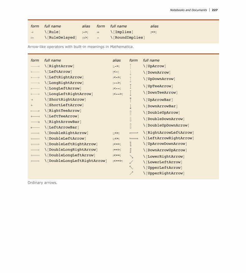
form full name aliasØ \@RuleD Ç->Ç

ß \@RuleDelayedD Ç:>Ç

form full name aliasfl \@ImpliesD Ç=>Ç

V \@RoundImpliesD

Arrow-like operators with built-in meanings in Mathematica.

form full name alias\@RightArrowD Çâ->Ç

\@LeftArrowD Ç<-Ç

\@LeftRightArrowD Ç<->Ç

\@LongRightArrowD Ç-->Ç

\@LongLeftArrowD Ç<--Ç

\@LongLeftRightArrowD Ç<-->Ç

z \@ShortRightArrowDy \@ShortLeftArrowD

\@RightTeeArrowD\@LeftTeeArrowD\@RightArrowBarD\@LeftArrowBarD\@DoubleRightArrowD Çâ=>Ç

\@DoubleLeftArrowD Çâ<=Ç

\@DoubleLeftRightArrowD Ç<=>Ç

\@DoubleLongRightArrowD Ç==>Ç

\@DoubleLongLeftArrowD Ç<==Ç

\@DoubleLongLeftRightArrowD Ç<==>Ç

form full name\@UpArrowD

\@DownArrowD

\@UpDownArrowD

\@UpTeeArrowD

\@DownTeeArrowD

\@UpArrowBarD

\@DownArrowBarD

\@DoubleUpArrowD

\@DoubleDownArrowD

\@DoubleUpDownArrowD

\@RightArrowLeftArrowD\@LeftArrowRightArrowD\@UpArrowDownArrowD

\@DownArrowUpArrowD

é \@LowerRightArrowDã \@LowerLeftArrowDå \@UpperLeftArrowDç \@UpperRightArrowD

Ordinary arrows.


form full name alias\@RightVectorD ÇvecÇ

\@LeftVectorD\@LeftRightVectorD\@DownRightVectorD\@DownLeftVectorD\@DownLeftRightVectorD\@RightTeeVectorD\@LeftTeeVectorD\@DownRightTeeVectorD\@DownLeftTeeVectorD\@RightVectorBarD\@LeftVectorBarD\@DownRightVectorBarD\@DownLeftVectorBarD\@EquilibriumD ÇequiÇ

\@ReverseEquilibriumD

form full name\@LeftUpVectorD

\@LeftDownVectorD

\@LeftUpDownVectorD

\@RightUpVectorD

\@RightDownVectorD

\@RightUpDownVectorD

\@LeftUpTeeVectorD

\@LeftDownTeeVectorD

\@RightUpTeeVectorD

\@RightDownTeeVectorD

\@LeftUpVectorBarD

\@LeftDownVectorBarD

\@RightUpVectorBarD

\@RightDownVectorBarD

\@UpEquilibriumD

\@ReverseUpEquilibriumD

Vectors and related arrows.

All the arrow and vector-like operators in Mathematica are infix.

In[6]:= x F y z

Out[6]= x F y z

form full name alias¢ \@RightTeeD ÇrTÇ

§ \@LeftTeeD ÇlTÇ

¶ \@UpTeeD ÇuTÇ

ß \@DownTeeD ÇdTÇ

form full name£ \@DoubleRightTeeD• \@DoubleLeftTeeD

Tees.


Structural Elements and Keyboard Characters

full name alias

\@InvisibleCommaD Esc ,Esc

\@InvisibleApplicationD Esc @Esc

\[InvisibleSpace] Esc isEsc

\@ImplicitPlusD Esc +Esc

full name alias

\[AlignmentMarker] Esc amEsc

\[NoBreak] Esc nbEsc

\[Null] Esc nullEsc

Invisible characters.

In the input there is an invisible comma between the 1 and 2.

In[1]:= m12

Out[1]= m1,2

Here there is an invisible space between the x and y, interpreted as multiplication.

In[2]:= FullForm@xyD

Out[2]//FullForm= Times@x, yD

\[Null] does not display, but can take modifications such as superscripts.

In[3]:= f@x, ^aD

Out[3]= fAx, aE

The \[AlignmentMarker] does not display, but shows how to line up the elements of the column.

In[4]:= Grid@88"b + c + d"<, 8"a + b + c"<<, Alignment -> ""D êê DisplayForm

Out[4]//DisplayForm=b + c + d

a + b + c

The \@ImplicitPlusD operator is used as a hidden plus sign in mixed fractions.

In[5]:= 12

3

Out[5]=5

3


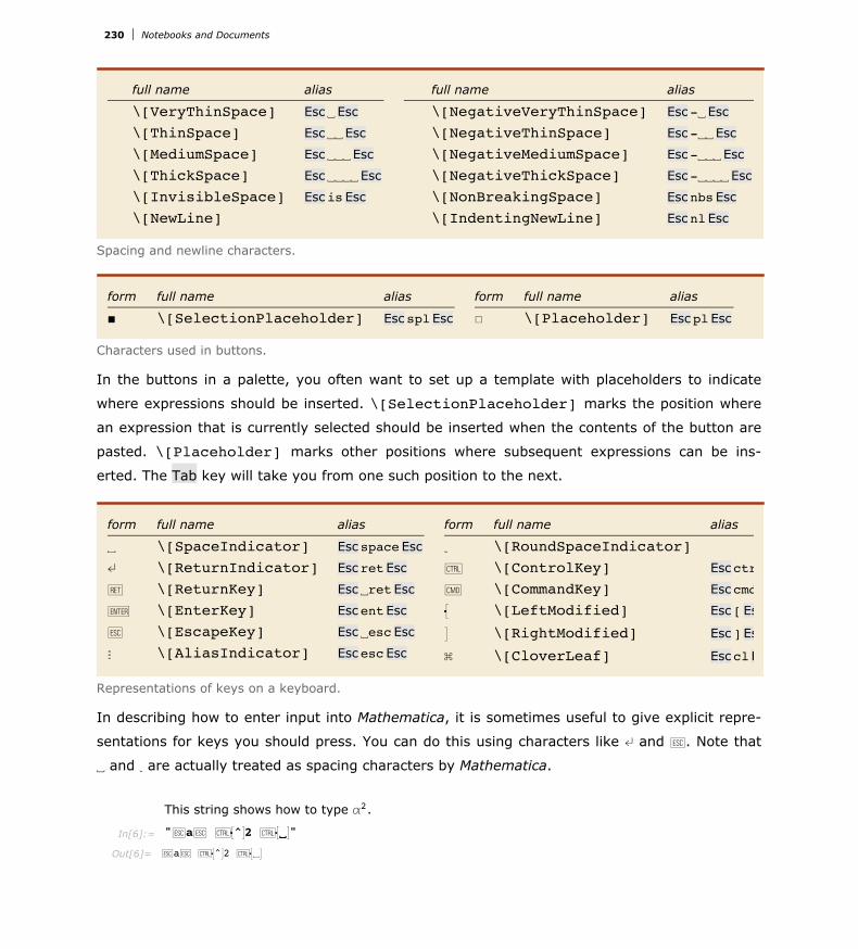
full name alias

\[VeryThinSpace] Esc âEsc

\[ThinSpace] Esc ââEsc

\[MediumSpace] Esc âââEsc

\[ThickSpace] Esc ââââEsc

\[InvisibleSpace] Esc isEsc

\[NewLine]

full name alias

\[NegativeVeryThinSpace] Esc -âEsc

\[NegativeThinSpace] Esc -ââEsc

\[NegativeMediumSpace] Esc -âââEsc

\[NegativeThickSpace] Esc -ââââEsc

\[NonBreakingSpace] Esc nbsEsc

\[IndentingNewLine] Esc nlEsc

Spacing and newline characters.


É \[SelectionPlaceholder] Esc splEsc


Ñ \[Placeholder] Esc plEsc

Characters used in buttons.

In the buttons in a palette, you often want to set up a template with placeholders to indicate

where expressions should be inserted. \[SelectionPlaceholder] marks the position where

an expression that is currently selected should be inserted when the contents of the button are

pasted. \[Placeholder] marks other positions where subsequent expressions can be ins-

erted. The Tab key will take you from one such position to the next.


â \[SpaceIndicator] Esc spaceEsc

¿ \[ReturnIndicator] Esc retEsc

Á \[ReturnKey] Esc âretEsc

Û \[EnterKey] Esc entEsc

Â \[EscapeKey] Esc âescEsc

Ç \[AliasIndicator] Esc escEsc


Ô \[RoundSpaceIndicator]‚ \[ControlKey] Esc ctrlEsc

· \[CommandKey] Esc cmdEsc

Î \[LeftModified] Esc [Esc

Ï \[RightModified] Esc ]Esc

Ì \[CloverLeaf] Esc clEsc

Representations of keys on a keyboard.

In describing how to enter input into Mathematica, it is sometimes useful to give explicit repre-

sentations for keys you should press. You can do this using characters like ¿ and Â. Note that

â and Ô are actually treated as spacing characters by Mathematica.

This string shows how to type a2.

In[6]:= "ÂaÂ ‚Î^Ï2 ‚ÎâÏ"

Out[6]= ÂaÂ ‚Î^Ï2 ‚ÎâÏ


form full name

Ö \[Continuation]á \@LeftSkeletonDà \[RightGuillemet]

form full name

Ü \[SkeletonIndicator]› \[ErrorIndicator]

Characters generated in Mathematica output.

Mathematica uses a \[Continuation] character to indicate that the number continues onto the next line.

In[7]:= 80!

Out[7]= 71569457046263802294811533723186532165584657342365752577109445058227039255480148842Ö668944867280814080000000000000000000

form full name

\[RawTab]\[NewLine]\[RawReturn]\[RawSpace]

! \@RawExclamationD" î @RawDoubleQuoteD

Ò \@RawNumberSignD$ \[RawDollar]% \@RawPercentD& \@RawAmpersandD' \@RawQuoteDI \@RawLeftParenthesisD

M \@RawRightParenthesisD

* \@RawStarD+ \@RawPlusD, \@RawCommaD- \@RawDashD. \@RawDotD

form full name

ë \@RawSlashD

: \@RawColonD; \@RawSemicolonD< \@RawLessD= \@RawEqualD> \@RawGreaterD? \@RawQuestionDü \@RawAtDA \@RawLeftBracketD

\ \@RawBackslashDE \@RawRightBracketD

^ \@RawWedgeD_ \[RawUnderscore]

` \[RawBackquote]9 \@RawLeftBraceD

\@RawVerticalBarD

= \@RawRightBraceD

~ \@RawTildeD

Raw keyboard characters.

The fonts that are distributed with Mathematica contain their own renderings of many ordinary

keyboard characters. The reason for this is that standard system fonts often do not contain

appropriate renderings. For example, ^ and ~ are often drawn small and above the centerline,

while for clarity in Mathematica they must be drawn larger and centered on the centerline.


Mathematica Tutorial: Notebooks And Documents - Wolfram Research

Documents

Transcript of Mathematica Tutorial: Notebooks And Documents - Wolfram Research