Time Series Outlier Analysis: Evidence for Management and Environmental Influences on Sockeye Salmon Catches

in Alaska and Northern British Columbia

Edward V. Farley, Jr., and James M. Murphy

Reprinted from the Alaska Fishery Research Bulletin

Vol. 4 No. 1, Summer 1997

36 Articles

Alaska Fishery Research Bulletin 4(1):36–53. 1997.

Time Series Outlier Analysis: Evidence for Management and Environmental Influences on Sockeye Salmon Catches

in Alaska and Northern British Columbia

Edward V. Farley, Jr., and James M. Murphy

ABSTRACT: Autoregressive, moving average models were fit and outliers were identified for commercial catches of 9 major sockeye salmon Oncorhynchus nerka stocks in Alaska and northern British Columbia. Distinct patterns in the sample autocorrelation and partial autocorrelation functions indicated stock-specific dynamics. Three types of outliers were considered: level-shift, temporary-change, and additive outliers. Most additive outliers were unex­plainable and may represent multiplicative survival at several different life history stages. Additive outliers that could be explained resulted from changes in fishing effort. Temporary-change outliers commonly reflected cold winter temperatures in western Alaska during the early 1970s. Four of nine river systems in our analysis had level-shift outliers, and only one of these had a positive shift in the late 1970s. The level-shift outliers, which indicate a long-term shift in catch levels, appeared to be the result of changes in escapement policy rather than an abrupt change in the production dynamics of the North Pacific.

INTRODUCTION

Sockeye salmon Oncorhynchus nerka catches in Alaska have fluctuated greatly over the last 60 years. Although there can be large year-to-year variation in catch levels, an obvious increasing trend is apparent in the commercial catch (Figure 1). Sockeye salmon catches reached their lowest levels between the mid 1940s and mid 1970s but recovered to record highs in the 1990s. This dramatic shift in salmon catches throughout Alaska has sparked renewed interest in ex­plaining and modeling the possible underlying mecha­nisms responsible for salmon catch trends.

The most recent analyses of Alaska salmon catch have used time series models. Hare and Francis (1995) used univariate models and intervention analyses for sockeye salmon of western and central Alaska and pink salmon O. gorbuscha in southeastern Alaska. Quinn and Marshall (1989) used univariate and multivariate time series analyses to model catch of pink and chum O. keta salmon in southeastern Alaska. Each study indi­cated an underlying environmental mechanism as the possible cause for dynamic trends in salmon produc­tion.

The focus of previous time series analyses has been on aggregate catch, either by species and region within Alaska (southeastern, central, and western) or total Alaska catch by species. Although aggregate salmon catches contain similar trends during the same peri­ods (Hare and Francis 1995), temporal patterns of catches, disaggregated by separate river systems or management units, may differ. Marshall and Quinn (1987) found patterns or trends in aggregate south­eastern Alaska salmon catch data that were difficult to interpret; they recommended analysis on disaggregated salmon catches.

Much of the difficulty in interpreting patterns in the aggregate catch is due to the inability to adequately separate variable effects of environment and manage­ment. The geographic scale of environmental influ­ences on salmon production can range from the entire North Pacific to local climate in freshwater rearing areas.

Direct management effects on salmon production are most easily interpreted for individual stocks or river systems, the functional unit often used in management. By maintaining a resolution in the catch data that most closely matches the resolution of management actions,

Authors: EDWARD V. FARLEY, JR., and JAMES M. MURPHY are currently under contract with TAG-Data Flow/Alaska, Inc., for the Ocean Carrying Capacity Program at Auke Bay Laboratory, Alaska Fisheries Science Center, National Marine Fisheries Service, 11305 Glacier Highway, Juneau, AK 99801. Acknowledgments: Jerome Pella, Steve Ignell, and Michelle Masuda — reviewed the manuscript. Ben Van Alen, Chris Hicks, and Beverly Cross — provided catch data. Project Sponsorship: National Marine Fisheries Service, Ocean Carrying Capacity Project provided monetary support under contract GS10K96ECD001.

36

37 Sockeye Salmon Time Series Outlier Analysis • Farley and Murphy

0.0

10.0

20.0

30.0

40.0

50.0

60.0

70.0

Cat

ch (

mill

ions

)

1928 1933 1938 1943 1948 1953 1958 1963 1968 1973 1978 1983 1988 1993

Year

Figure 1. Total Alaska sockeye salmon commercial catch, 1928–1996.

we can more effectively segregate the relative influ­ence of management and environment. In this paper, we examine sockeye salmon catch time series for 9 individual river systems from western, central, and southeastern Alaska and northern British Columbia by analyzing the relationship of data series outliers in terms of management strategies and environmental influences.

METHODS

Our approach to analyzing the catch time series was separated into 3 parts. First, we identified the appro­priate univariate model for each river system based on autocorrelation patterns (Box and Jenkins 1976). Then we simultaneously estimated the model parameters and detected the presence of outliers in each data series through an iterative procedure developed by Chen and Liu (1993). Last, we discussed each outlier in terms of management strategy and environmental influences.

Data

We modeled commercial catches of 9 sockeye salmon stocks aggregated into 3 regions: southeastern Alaska including British Columbia (BC), western Alaska, and central Alaska. Catch data for the 9 stocks were from the Skeena River (BC) and the Situk River in south­eastern Alaska; the Ugashik, Naknek/Kvichak, and Egegik Rivers in western Alaska (Bristol Bay); and the Alitak, Karluk, Chignik, and Copper Rivers in cen­tral Alaska (Table 1; Figure 2). Catch data were not available for the Egegik River in 1942, 1943, and 1945; for the Ugashik River in 1935; and for the Situk River in 1928, 1929, 1932, 1936, 1937, and 1960. Catch data

for the missing years were estimated by the average of the previous 5 annual catches. Catches were log-trans­formed (Figure 3) to stabilize variance in the catch; catches tended to have a skewed distribution and vari­ance increased as the mean increased.

Univariate Time Series Analysis

Univariate autoregressive integrated moving aver­age (ARIMA) modeling techniques (Box and Jenkins 1976) were used to reveal patterns and relationships in the sockeye salmon catch data. A 3-phase approach for identifying and fitting ARIMA models was used: (1) model identification, (2) estimation of model pa­rameters, and (3) diagnostics and model criticism. Autoregressive (AR) and moving average (MA) mod­els were fit to the data. In AR processes, the present value of a time series depends on preceding values plus a random shock. A pth order AR process, designated ARIMA p, , or AR p , is defined by0 0 ( )( )

Zt = ¢ Z + ¢ t− + + ¢ p t p Z + a , or1 t−1 2 Z 2 . − t

2 . p)(1− ¢ B− ¢ B − − ¢ B Z = a , (1)1 2 p t t

where ¢ j is the j th AR, Zt = (zt –f), f is the series mean, at is the Gaussian white-noise error term at time t , and B is the backward-shift operator where

pB Z( )t = Zt p . In MA processes, random events pro­-

duce an immediate effect that dissipates after short periods. The qth order MA model, designated as ARIMA( )0 0, , q or MA( )q , is defined by

Z = a − B a −1 − − B a −.t t 1 t q t q , or

t 22 . q ) t (2)Z = −(1 B1B−B B − − BqB a ,

where Bq is the q th MA parameter.

38 Articles

Table 1. References used to build the sockeye salmon catch data series for each river system.

River Years and Data Sources

Skeena 1928–1954a 1955–1967b 1968–1972c 1973–1984d 1985–1996e

Situk 1930–1949f 1951–1959g 1960–1996h

Copper 1928–1991i 1992–1994j 1995–1996k

Alitak 1928–1996l

Chignik 1928–1966m 1967–1987n 1988–1994o 1995–1996k

Karluk 1928–1996l

Ugashik 1928–1955p 1956–1995q 1996r

Naknek/Kvichak 1928–1955p 1956–1995q 1996r

Egegik 1928–1955p 1956–1995q 1996r

a Shepard and Withler (1958) b DFF (1970)c INPFC (1970 and through 1975)d DE (1974 and through 1979); DFO (1980 and through 1985)e Data for 1985–1996 c/o John Morris, Department of Fisheries and Oceans, Nanaimo, British Columbia f USDIFWS (1930 and through 1949)g Simpson (1960)h Data for 1960–1996 c/o Ben Van Alen, Alaska Department of Fish and Game, Juneau i Rigby et al. (1991)j Geiger and Savikko (1993); Geiger and Simpson (1994, 1995)k Buls (1996); Shapiro (1997)l Data for 1928–1996 c/o Chris Hicks, Alaska Department of Fish and Game, Kodiak m Dahlberg (1968) n Barrett (1989) o Savikko (1989); Savikko and Page (1990); Geiger and Savikko (1991, 1992, 1993); Geiger and Simpson (1994, 1995) p INPFC (1979) q Data for 1956–1995 c/o Beverly Cross, Alaska Department of Fish and Game, Anchorage r Alaska Department of Fish and Game web page — http://www.state.ak.us/adfg/cfmd/geninfo/finfish/salmon/salmhome.htm

Both AR and MA models required stationary time series, i.e., no trend in variance or mean values. Trends in mean values were removed by taking successive dif­ferences of the data, to create a new series z′ t , where z′ = t Zt − Zt−1. The number of differences required for a stationary series to evolve was denoted by d. Non-stationary variance was remedied by applying a loga­rithmic transformation (Vandaele 1983; Quinn 1985). Differencing operations and AR and MA models can be combined into a single model known as the autore­gressive, integrated, MA model, or ARIMA( )p d q ., ,The equation for the ARIMA( )p d q model is defined, ,by

2 p d(1− ¢1B− ¢2B −.− ¢ pB )( )1− B Zt =

C + − B B−B B −.− B B(1 2 q )a . (3)1 2 q t

The term C is related to the mean of the process when the original process is stationary, i.e., C= f�(1-¢ -.-¢ ) .1 p

Three functions were used in identifying time se­ries models: sample autocorrelation function (SACF), sample partial autocorrelation function (SPACF), and extended sample autocorrelation function (ESACF). The SACF measures the correlation between Zt and Zt k , where k is the time lag, whereas the SPACF quan­+ tifies the correlation between Zt and Zt k after their+mutual linear dependency on the intervening variables Z , Z . Z ) has been removed (Wei 1990). ( , ,t+ t+2 + − 11 t k

AR models are characterized by an exponential or os­cillatory decay of the SACF and one or more spikes at various lags in the SPACF. The opposite is true for MA models: decaying SPACF and spiked SACF. If the SACF decays very slowly and the SPACF cuts off after lag 1, the series is possibly nonstationary and requires a differencing operation (Wei 1990).

Mixed ARIMA models were identified using the ESACF (Tsay and Tiao 1984). The ESACF table is drawn with X for significant values and O for values that are within 2 standard errors of zero. Tentative models are identified by drawing a triangle whose

39 Sockeye Salmon Time Series Outlier Analysis • Farley and Murphy

25.00

20.00

15.00

10.00

5.00

0.00

Naknek/Kvichak

1928 1938 1948 1958 1968 1978 1988

Ugashik

8.00

6.00

4.00

2.00

0.00

1928 1938 1948 1958 1968 1978 1988

Karluk

1.20 1.00 0.80 0.60 0.40 0.20 0.00

1928 1938 1948 1958 1968 1978 1988

Copper

2.50 2.00 1.50 1.00 0.50 0.00

1928 1938 1948 1958 1968 1978 1988

Skeena

Egegik

25.00

20.00

15.00

10.00

5.00

0.00

1928 1938 1948 1958 1968 1978 1988

Chignik

3.00 2.50 2.00 1.50 1.00 0.50 0.00

1928 1938 1948 1958 1968 1978 1988

Alitak

2.50

2.00

1.50

1.00

0.50

0.00

1928 1938 1948 1958 1968 1978 1988

Situk

0.30

0.20

0.10

0.00

1928 1938 1948 1958 1968 1978 1988

Cat

ch (m

illio

ns)

0.00

1.00

2.00

3.00

4.00

1928 1938 1948 1958 1968 1978 1988

Year

Figure 2. Sockeye salmon commercial catch for 9 major sockeye salmon-producing rivers in Alaska and British Columbia, 1928–1996.

40 Articles

17.5

16.5

15.5

14.5

13.5

12.5

Naknek/Kvichak

1928 1938 1948 1958 1968 1978 1988

Ugashik

15.5

13.5

11.5

9.5

7.5

1928 1938 1948 1958 1968 1978 1988

Karluk

14.0 13.0 12.0 11.0 10.0 9.0 8.0

1928 1938 1948 1958 1968 1978 1988

Copper

15.0 14.0 13.0 12.0 11.0 10.0

9.0

Log

(Cat

ch)

1928 1938 1948 1958 1968 1978 1988

Skeena

15.5

Egegik

17.0

16.0

15.0

14.0

13.0

12.0

1928 1938 1948 1958 1968 1978 1988

Chignik

15.0

14.0

13.0

12.0

11.0

10.0

1928 1938 1948 1958 1968 1978 1988

Alitak

16.5

14.5

12.5

10.5

8.5

1928 1938 1948 1958 1968 1978 1988

Situk

13.5 12.5 11.5 10.5

9.5 8.5

1928 1938 1948 1958 1968 1978 1988

14.5

13.5

12.5

11.5

1928 1938 1948 1958 1968 1978 1988

Year

Figure 3. Sockeye salmon logarithm of commercial catch for 9 major sockeye salmon-producing rivers in Alaska and British Columbia, 1928–1996.

Additive Outlier

Temporary Change Outlier

Level Shift Outlier

41 Sockeye Salmon Time Series Outlier Analysis • Farley and Murphy

vertex is in the position p q so that all O values in 1( , 0 )0 the table are for the ( )i j coordinates in the triangular 0.9 ,

0.8 Additive Outlier

Temporary-Change Outlier

Level-Shift Outlier

region, where i p k= and j q k, k , , ,…0 + ≥ 0 + = 0 1 20.7

Examples of ESACF use are found in Tsay and Tiao (1984), Quinn and Marshall (1989), Wei (1990), and Farley (1996). E

ffect

0.6

0.5

0.4

Model parameters were estimated using the maxi­mum likelihood method. The significance of the model parameters was determined by constructing a test sta­tistic defined by t , the estimate minus the hypothesized value divided by the estimated standard deviation of the estimate.

This statistic was compared to the critical value of the t distribution for the 5% level with ( )n p− de­grees of freedom. In general, the hypothesis, ¢p or Bq = 0 , was rejected when the t value was >1.7 (n≤ 70) . Diagnostic checks were performed to assess model adequacy by checking whether the model as­sumptions were satisfied. The basic assumption is that the {at } values were uncorrelated random shocks with a zero mean and constant variance (Wei 1990). The sample ACF and PACF of the {at } values were used to determine if the residuals showed any patterns and that autocorrelation at all lags were statistically insig­nificant (within 2 standard deviations at the 5% level). The presence of large autocorrelations in the SACF of the residuals indicated the model was inadequate.

Outlier Detection

Three types of outliers were considered, including ad­ditive outliers (AO), level shifts (LS), and temporary changes (TC; Chen and Liu 1993; Figure 4). An AO is a pulse that affects the time series at one period only. An LS is an event that permanently affects the subse­quent level of a series. A TC is an event that decays exponentially according to a prespecified dampening factor.

The AO, LS, and TC occurring at time t T can=be represented as

( )TAO: Y Z t = + wA t t P ( )TLS: Y Z = + w St t L t

1 ( )TTC: Y Z = + w P , (4)t t c t1− 8B Twhere Pt

( ) is referred to as a pulse function repre­sented in a binary fashion, assuming the value 1 when

Tt T= and 0 otherwise, and St ( ) is referred to as a step

function represented in a binary fashion, assuming the value 0 before t T and the value 1 thereafter. The =values for w w, , and w represent the deviation fromA L c,

0.3

0.2

0.1

0

1 2 3 4 5 6 7 8 9 10 11 12 13 14

Time

Figure 4. Plot illustrating the effect of an additive outlier, temporary-change outlier with 8 = 0.7, and level-shift outlier on later periods.

the prior value of ZT , and the 8 parameter is the damp­ening factor, which can be specified by the analyst but is given a default value of 0.7 (Chen and Liu 1993).

After an ARIMA model was identified, model pa­rameters and outliers within the time series were jointly estimated by an iterative procedure (Chen and Liu 1993). Outliers were detected by calculating 3 test sta­tistics, 1 for each type of outlier. The largest test sta­tistic (in absolute value) for each outlier type was re­tained and compared with a prespecified critical value. Chen and Liu (1993) suggest a critical value of 3.0 for data series with lengths between 100 and 200; for data series <100, they suggest a critical value between 2.5 and 2.9. However, they point out that spurious outli­ers, or the presence of a large number of outliers, may appear when the critical value is too low, and they em­phasize the need to validate the outliers through re­sidual plots. We selected the lowest critical value that did not produce spurious outliers and resulted in an adequate model fit. Adequacy of the model fit was evaluated by both the residual pattern and the stan­dard errors of the model parameters.

RESULTS

Univariate Models

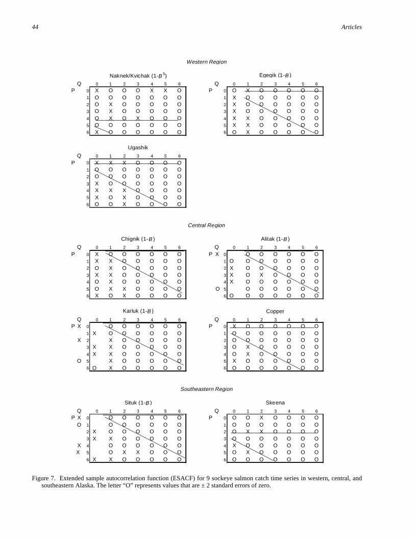
For Naknek/Kvichak (western Alaska), autocorrela­tion at lags 1 and 5 in the SACF and lags 1, 2, 4, and 6 in the SPACF were significant (Figure 5). The com­plexity of the autocorrelation function indicated a pos­sible need to difference the data. Differencing the data by 5 produced a less complex autocorrelation func­tion and suggested a possible ARIMA(5,5,0) (Fig­ure 6). The ESACF for differenced data (Figure 7) also suggested a possible ARIMA(5,5,0) model for the

42 Articles

Naknek/ 1.0 0.5

Kvichak 0.0 -0.5 -1.0

Egegik 1.0 0.5 0.0

-0.5 -1.0

Ugashik 1.0 0.5 0.0

-0.5 -1.0

Chignik 1.0 0.5 0.0

-0.5 -1.0

1.0 Alitak 0.5

0.0 -0.5 -1.0

1.0 Karluk 0.5

0.0 -0.5 -1.0

1.0 Copper 0.5

0.0 -0.5 -1.0

1.0 Situk 0.5

0.0 -0.5 -1.0

1.0 Skeena 0.5

0.0 -0.5 -1.0

SACF SPACF

Western Region

1.0 0.5 0.0

-0.5 -1.0

1.0 0.5 0.0

-0.5 -1.0

1.0 0.5 0.0

-0.5 -1.0

Central Region

1.0 0.5 0.0

-0.5 -1.0

1.0 0.5 0.0

-0.5 -1.0

1.0 0.5 0.0

-0.5 -1.0

1.0 0.5 0.0

-0.5 -1.0

Southeastern Region

1.0 0.5 0.0

-0.5 -1.0

1.0 0.5 0.0

-0.5 -1.0

1 2 3 4 5 6 7 8 9 10 1 2 3 4 5 6 7 8 9 10

Lag

Figure 5. Sample autocorrelation function (SACF) and sample partial autocorrelation function (SPACF) for 9 sockeye salmon catch time series in western, central, and southeastern Alaska. Horizontal dashed lines represent ± 2 standard errors of the sample lag autocorrelation estimates.

43 Sockeye Salmon Time Series Outlier Analysis • Farley and Murphy

Naknek/Kvichak sockeye salmon catch series. The sen for the Naknek/Kvichak sockeye salmon catch (Ta­ARIMA(5,5,0) model fit to the data series resulted in ble 2). statistically insignificant AR terms for lags 2, 3, and For Egegik (western Alaska), the SACF decayed 4. Analysis of the residuals indicated serial correla- slowly, indicating the series needed to be differenced tion had been adequately accounted for by the model. (Figure 5). Differencing the series by 1 produced an Therefore, the ARIMA(5,5,0) ¢2 4 0 SACF that cut off after lag 4 and an SPACF that con­− = model was cho-

SACF SPACF

Western Region

1.0 1.0 Naknek/

0.5 0.5 Kvichak 0.0 0.0

-0.5 -0.5

-1.0 -1.0

1.0 1.0 Egegik

0.5 0.5

0.0 0.0

-0.5 -0.5

-1.0 -1.0

Central Region

1.0 1.0 Chignik

0.5 0.5

0.0 0.0

-0.5 -0.5

-1.0 -1.0

0.5 0.5 Alitak

0.0 0.0

-0.5 -0.5

-1.0 -1.0

1.0 1.0 Karluk

0.5 0.5

0.0 0.0

-0.5 -0.5

-1.0 -1.0

Southeastern Region

1 2 3 4 5 6 7 8 9 10 1 2 3 4 5 6 7 8 9 10

Lag

-1.0

-0.5

0.0

0.5

1.0

-1.0

-0.5

0.0

0.5

1.0 Situk

Figure 6. Sample autocorrelation function (SACF) and sample partial autocorrelation function (SPACF) of the differentiated sockeye salmon catch time series in western, central, and southeastern Alaska. Horizontal dashed lines represent ± 2 standard errors of the sample lag autocorrelation estimates.

44 Articles

Western Region

Naknek/Kvichak (1-B 5) Egegik (1-B )

Q 0 1 2 3 4 5 6 Q 0 1 2 3 4 5 6

P 0 X O O O X X O P 0 O X O O O O O 1 1O O O O O O O X O O O O O O 2 O X O O O O O X O O O O O O 3

2

O X O O O O O 3 X O O O O O O 4 O X O X O O O X X O O O O O 5

4

O O O O O O O X X O O O O O 6

5

6X O O O O O O O X O O O O O

Ugashik

Q 0 1 2 3 4 5 6

P 0 X X X O O O O 1 O O O O O O O 2 O O O O O O O 3 X O O O O O O 4 X X X O O O O 5 X O X O O O O 6 O O X O O O O

Central Region

Chignik (1-B ) Alitak (1-B )

Q 0 1 2 3 4 5 6 Q 0 1 2 3 4 5 6

P 0 X O O O O O O P 0 X O O O O O O 1 X X O O O O O O O O O O O O 2

1

2O X O O O O O X O O O O O O 3 X X O O O O O X O X O O O O 4

3

O X O O O O O X O O O O O O 5

4

O X X O O O O 5 O O O O O O O 6 X O X O O O O O O O O O O O6

Karluk (1-B ) Copper

Q 0 1 2 3 4 5 6 Q 0 1 2 3 4 5 6

P 0 X O O O O O O P 0 X O O O O O O 1 1X O O O O O O O O O O O O O 2 X X O O O O O O O O O O O O 3

2

X X O O O O O O X O O O O O 4

3

X X O O O O O 4 O X O O O O O 5 O X O O O O O X O O O O O O 6

5

6O X O O O O O O O O O O O O

Southeastern Region

Situk (1-B ) Skeena

Q 0 1 2 3 4 5 6 Q 0 1 2 3 4 5 6

P 0 X O O O O O O P 0 O O X O O O O 1 O O O O O O O O O O O O O O 2

1

X O O O O O O 2 O X X O O O O 3 3X X O O O O O O O O O O O O 4 X O O O O O O 4 X O O O O O O 5 X O X X O O O O X O O O O O 6

5

X X O O O O O O O O O O O O6

Figure 7. Extended sample autocorrelation function (ESACF) for 9 sockeye salmon catch time series in western, central, and southeastern Alaska. The letter “O” represents values that are ± 2 standard errors of zero.

45 Sockeye Salmon Time Series Outlier Analysis • Farley and Murphy

Table 2. Parameter and adjusted parameter estimates, T values in parentheses, and residual standard errors (RSE) for both univariate time series models (ARIMA) and models that include outliers.

River ARIMA Model

Univariate Parameter Estimates RSE

Outlier Parameter Estimates RSE

Naknek/ Kvichak

(5,5,0) ¢2,4=0 ¢1 = ¢5 =

0.48 (4.8) –0.37 (-3.7)

0.780 ¢1 = ¢5 =

0.50 (5.5) –0.44 (-4.8)

0.724

Egegik (5,1,1) ¢1–4=0

B1

= ¢

5 =

0.53 (4.9) 0.34 (2.9)

0.592 B1

= ¢

5 =

0.52 (4.7) 0.43 (3.7)

0.525

Ugashik (1,0,0) ¢1

= C =

0.74 (8.7) 13.28 (27.2)

1.056 ¢1

= C =

0.31 (2.5) 13.15 (125.8)

0.591

Chignik (0,1,1) B1 = 0.80 (10.4) 0.714

Alitak (0,1,1) B1

= 0.41 (3.7) 0.668 B1

= 0.35 (3.0) 0.442

Karluk (0,1,1) B1

= 0.72 (8.4) 0.923 B1

= 0.78 (9.1) 0.474

Copper (1,0,0) ¢1 = C =

0.43 (3.8) 13.30 (92.4)

0.679 ¢1 = C =

0.25 (1.9) 13.30 (226.5)

0.364

Situk (0,1,1) B1

= 0.39 (3.5) 0.471 B1

= 0.49 (4.6) 0.413

Skeena (3,0,0) ¢2 = 0

¢1

= ¢

3 =

C =

0.26 (2.3) 0.36 (3.2) 13.48 (70.7)

0.585 ¢

3 =

C = 0.36 (2.9) 13.56 (134.7)

0.524

tained significant autocorrelation at lags 1 and 5, sug­gesting a possible ARIMA(5,1,0). The ESACF of the differenced series suggested a possible ARIMA(1,1,1) for the series (Figure 7). The ARIMA(1,1,1) model fit to the data series produced a statistically insignificant AR term for lag 1. The residual analysis of the ARIMA (0,1,1) model contained significant correlation at lag 5. The ARIMA(5,1,1) model fit to the data produced statistically insignificant AR terms for lags 1 through 4. The residual analysis of the ARIMA(5,1,1) ¢1 4 0− = model indicated serial correlation had been adequately accounted for by the model. Therefore, the ARIMA (5,1,1) ¢1 4 0− = was chosen for this series (Table 2).

For Ugashik (western Alaska), the SACF and SPACF indicated a possible ARIMA(1,0,0) model for the series (Figure 5). The ESACF also suggested a possible ARIMA(1,0,0) model for the sockeye salmon catch series (Figure 7). The ARIMA(1,0,0) model fit to the data series produced a statistically significant AR term for lag 1. Analysis of the residuals indicated that serial correlation for the series was adequately ac­counted for by the model. Therefore, the ARIMA(1,0,0) model was chosen for this series (Table 2).

For Chignik (central Alaska), the SACF decayed slowly, indicating the series should be differenced

(Figure 5). Differencing the series by 1 produced an SPACF that decayed exponentially and an SACF that contained statistically significant correlation at lag 1 (Figure 6), suggesting a possible ARIMA(0,1,1). The ESACF of the differenced series also indicated a pos­sible ARIMA(0,1,1) model (Figure 7). The ARIMA (0,1,1) model fit to the data series produced a signifi­cant MA term for lag 1. Analysis of the residuals for the ARIMA(0,1,1) model indicated that serial corre­lation was adequately accounted for by the model. Therefore, the ARIMA(0,1,1) model was chosen for this series (Table 2).

For Alitak (central Alaska), the SACF decayed slowly, indicating the series should be differenced (Fig­ure 5). Differencing the series by 1 produced an SPACF that decayed exponentially and an SACF that contained significant correlation at lag 1 (Figure 6), suggesting a possible ARIMA(0,1,1). The ESACF for the differ­enced series also indicated a possible ARIMA(0,1,1) model (Figure 7). The ARIMA(0,1,1) produced an adequate model, and analysis of the residuals indicated no other serial correlation. Therefore, the ARIMA (0,1,1) model was chosen for this series (Table 2).

For Karluk (central Alaska), the SACF decayed slowly, indicating the series should be differenced

46 Articles

(Figure 5). The SACF and SPACF of the differenced 1− B( ) series indicated a possible ARIMA(0,1,1)

model for the series (Figure 6). The ESACF of the dif­ferenced series also suggested a possible ARIMA (0,1,1) model for the series (Figure 7). The ARIMA (0,1,1) produced an adequate model, and analysis of the residuals indicated no other serial correlation for the model. Therefore, the ARIMA(0,1,1) model was cho­sen for the Karluk sockeye salmon catch (Table 2).

For Copper (central Alaska), the SACF and SPACF patterns were slightly different from the 3 other river systems in central Alaska. The SACF did not slowly decay but cut off after lag 1, and the SPACF also con­tained significant correlation at lag 1 (Figure 5). The ESACF indicated an ARIMA(1,0,0) model for the se­ries (Figure 7). The ARIMA(1,0,0) model fit to the data series produced a significant AR term for lag 1. The residual analysis indicated no other serial corre­lation for the model. Therefore, the ARIMA(1,0,0) model was chosen for this series (Table 2).

For Situk (southeastern Alaska), the SACF de­cayed slowly, indicating the series should be differ­enced (Figure 5). The SACF and SPACF of the dif­ferenced series ( )1− B indicated a possible ARIMA (0,1,1) (Figure 6). The ESACF of the differenced se- 20.0

ries also suggested a possible ARIMA(0,1,1) model 15.0

(Figure 7). The ARIMA(0,1,1) model fit to the data series produced a significant MA term for lag 1. 10.0

Analysis of the residuals indicated the serial correla­ 5.0

tion had been adequately accounted for by the model. 0.0

Therefore, an ARIMA(0,1,1) was chosen for Situk (Table 2).

For Skeena (southeastern Alaska), the SACF and 25.0

SPACF contained significant lags 1 and 3 (Figure 5), and the ESACF indicated a possible ARIMA(3,0,0) model (Figure 7). Fitting an ARIMA(3,0,0) model to the Skeena sockeye salmon catch series produced an insignificant AR term for lag 2. Removing the AR C

atch

(m

illio

ns)

20.0

15.0

10.0

5.0

term for lag 2 and analyzing the residuals from the fitted ARIMA(3,0,0) ¢2 0 model indicated the serial

0.0

=correlation had been adequately accounted for by the model. Therefore, an ARIMA(3,0,0) ¢2 0 was chosen 7.0

6.0for Skeena (Table 2). =

5.0

4.0

Outlier Analysis 3.0

2.0

For Naknek/Kvichak (western Alaska), the iterative 1.0

outlier search produced a positive additive outlier for 0.0

Ugashik

LS AO

TC TC AOAO

Naknek/Kvichak AO

Egegik

AOAO

1983 (Table 3). The addition of the outlier to the time series model reduced the residual standard error by 7% over the univariate model (Table 2). The additive outlier in 1983 (Figure 8) did not correspond to any major shift in catch. However, the large catch in 1983

occurred for an off-cycle year and stands out as an outlier in the residual series because the ARIMA model, which accounts for the 5-year cycle, could not explain it.

For Egegik (western Alaska), 2 outliers were de­tected and jointly estimated with the model param­eters. A positive additive outlier was identified for 1961 and a negative additive outlier was identified for 1974 (Figure 8; Table 3). The addition of the outliers to the time series model reduced the residual standard error by 11% over the univariate model (Table 2).

For Ugashik (western Alaska), more than 10 out­liers were identified using the critical value of 2.6, and some appeared to be spurious. A critical value of 2.7 reduced the number of outliers and gave more credence to the results. The outliers identified include negative additive outliers for 1940, 1941, and 1978; negative temporary changes in 1972 and 1974; and a positive level shift in 1979 (Figure 8; Table 3). The inclusion of outliers greatly improved the fit of the time series

25.0

1928 1933 1938 1943 1948 1953 1958 1963 1968 1973 1978 1983 1988 1993

Year

Figure 8. Western Alaska sockeye salmon catch, 1928–1996; level shift (LS), temporary change (TC), and additive out­liers (AO) are identified for each river system.

47 Sockeye Salmon Time Series Outlier Analysis • Farley and Murphy

Table 3. Dates, parameter estimates, T values {date (estimate; T value)}, and critical values for the level shift (LS), temporary change (TC), and additive outliers (AO) identified for each sockeye salmon catch time series.

River Critical Value LS

Outliers TC AO

Naknek/ Kvichak

[2.6] 1983 (1.86; 3.3)

Egegik [2.6] 1961 (1.36; 3.3) 1974 (-1.35; -3.2)

Ugashik [2.7] 1979 (1.74; 8.8) 1972 (–3.05; –5.6) 1974 (–3.48; –6.3)

1940 (-2.74; -4.7) 1941 (-2.15; -3.6) 1978 (-2.63; -4.6)

Alitak [2.6] 1957 (–1.36; –3.3) 1967 (–1.68; –4.1) 1972 (–1.85; –4.4) 1992 (–1.19; –2.9)

1973 (-1.79; -4.8) 1975 (-1.57; -4.3)

Karluk [2.6] 1951 (–1.22; -4.1) 1971 (–1.40; –3.5) 1990 (1.67; 3.9)

1947 (–1.52; –3.3) 1955 (–1.95; –4.3) 1973 (–1.29; –2.8) 1989 (–4.24; –9.2)

Copper [2.9] 1982 (0.58; 4.8) 1935 (–1.87; –5.3) 1948 (–1.05; –3.0) 1979 (–1.78; –4.9) 1980 (–3.38; –9.3)

Situk [2.6] 1987 (1.74; 4.8)

Skeena [2.6] 1955 (–1.97; –4.9)

model and reduced the residual standard error by 44% (Table 2).

For Chignik (central Alaska), no outliers were de­tected.

For Alitak (central Alaska), negative additive out­liers were found for 1973 and 1975, as well as nega­tive temporary changes for 1957, 1967, 1972, and 1992 (Figure 9; Table 3). The inclusion of outliers in the time series model reduced the residual standard error by 34% over the univariate time series model (Table 2).

For Karluk (central Alaska), negative additive out­liers were found for 1947, 1955, 1973, and 1989; both negative and positive temporary changes were found for 1971 and 1990, respectively; and a negative level shift was found for 1951 (Figure 9; Table 3). The drop in catch for 1989 can be attributed to loss of fishing due to the Exxon Valdez oil spill. Inclusion of the out­liers in the time series model reduced the residual stan­

dard error by 48% over the univariate time series model (Table 2).

For Copper (central Alaska), analysis of the re­siduals from the outlier analysis with a critical value of 2.6 suggested an inadequate ARIMA model for the series. After estimating several different ARIMA models and analyzing residuals, an appropriate model could not be found. Increasing the critical value to 2.9 stabilized the model and produced satisfactory param­eter estimates and residuals. Negative additive outli­ers were found for 1935, 1948, 1979, and 1980, and a positive level shift was identified for 1982 (Figure 9; Table 3). The inclusion of outliers to the time series model greatly improved the residual standard error, reducing the residual standard error to 46% of the univariate time series model (Table 2).

For Situk (southeastern Alaska), a positive level shift was identified for 1987 (Figure 10; Table 3). The residual standard error for the time series model was

2.5

48 Articles

Chignik

0.0

0.5

1.0

1.5

2.0

2.5

3.0

Alitak

0.0

0.5

1.0

1.5

2.0

2.5

AOTCTC AOTC

TC

Karluk

0.0

0.2

0.4

0.6

0.8

1.0

1.2

LS

AO

AO

AO AO

TC

TC

Cat

ch (

mill

ions

)

0.0

0.1

0.1

0.2

0.2

0.3

0.3

AO

LS

Situk

Cat

ch (

mill

ions

)

0.0

0.5

1.0

1.5

2.0

2.5

3.0

3.5

TC

Skeena

1928 1933 1938 1943 1948 1953 1958 1963 1968 1973 1978 1983 1988 1993

Year

Figure 10. Southeastern Alaska sockeye salmon catch, 1928– 1996; level shift (LS), temporary change (TC), and additive outliers (AO) are identified for each river system.

DISCUSSION

0.0

0.5

1.0

1.5

2.0

1928 1933 1938 1943 1948 1953 1958 1963 1968 1973 1978 1983 1988 1993

Year

LS

AO

AO

AO AO

Copper

Alaska Salmon Production

Figure 9. Central Alaska sockeye salmon catch, 1928–1996; level shift (LS), temporary change (TC), and additive out­liers (AO) are identified for each river system.

reduced by 12% when the outliers were included in the time series model (Table 2).

For Skeena (southeastern Alaska), the outlier iden­tification process with a critical value of 2.6 suggested a different model from the previous ARIMA(3,0,0)

model. The AR term for lag 1 became insignifi­¢2 0= cant after the outliers in the model were estimated. The outlier search for the ARIMA(3,0,0) ¢1 2 0 model , =identified a negative temporary-change outlier for 1955 (Figure 10; Table 3). The residual standard error was reduced by 10% when the outlier was included in the time series model (Table 2).

Over the past 60 years, sockeye salmon catches have fluctuated widely from a low of roughly 4.5 million in 1973 to >64 million in 1993 (Figure 1). Changes in both management policy and environmental conditions have been hypothesized as contributing factors in these fluctuations.

Management policies affecting catch levels include variable escapement strategies (Eggers et al. 1984), high seas interceptions (Eggers et al. 1984; Rogers 1984; Pella et al. 1993), improved access to spawning grounds (Van Cleve and Bevan 1973), lake fertility (Stockner 1987), and direct manipulation of spawn­ing ground habitat (Sprout and Kadowaki 1987; West and Mason 1987). Environmental influences on catch range in scale from changes in regional climatic con­ditions, such as winter air temperatures (Mathisen and Poe 1981; Eggers et al. 1984; Rogers 1984), to ocean basin-scale shifts in the North Pacific environment (Mysak 1986; Francis and Hare 1994; Beamish and Bouillon 1995; Hare and Francis 1995).

Basin-scale climatological conditions in the Gulf of Alaska are related to the intensity of the Aleutian Low Pressure System: greater intensity corresponds with increased precipitation (Cayan and Petersen 1989), wind stress and Eckman transport (Thompson

49 Sockeye Salmon Time Series Outlier Analysis • Farley and Murphy

1981; Trenberth 1991), and vertical mixing (Thomp­son 1981; Lau 1988; Rogers and Raphael 1992), all of which may provide linkages between basin-scale cli­mate and salmon production. Evidence for linkages between salmon production and the intensity of the Aleutian Low can be seen in their parallel decrease in the late 1940s and increase in the late 1970s (Beam­ish and Bouillon 1995).

Hare and Francis (1995) hypothesized the sock­eye salmon catch in western and central Alaska was impacted by a large-scale climate change reflected in North Pacific atmospheric-oceanic regime shifts dur­ing 1946–1947 and 1976–1977. They used interven­tion analysis to determine if significant level shifts were present in Alaska sockeye salmon catches. Neg­ative level shifts in western and central Alaska sock­eye salmon occurred during 1949 and 1950, and pos­itive level shifts occurred during 1979 and 1980. Hare and Francis (1995) concluded level shifts found in sockeye salmon catches imply an abrupt change or “snap” in the biological production dynamics of the North Pacific.

The impact of large-scale climate shifts in the marine environment has important implications for fisheries management. Increased escapements or arti­ficial enhancement can be successful in increasing catch levels during favorable regime shifts; however, attempts to rebuild stocks through increased escape­ments or artificial enhancement are unlikely to be suc­cessful during periods of low ocean productivity. To effectively evaluate management policies regarding escapement and artificial enhancement, it is impor­tant to recognize changes in productivity regimes in the oceanic environment (Beamish et al. 1997). For example, forecasts produced for sockeye salmon re­turns to Bristol Bay omit data prior to 1978 because models based on most recent data more accurately reflect current trends in sockeye salmon production (Cross et al. 1993).

Analyses comparing large-scale climate shifts to sockeye salmon production have been based prima­rily on aggregate catch levels. However, stock-specific production dynamics play an important role in deter­mining catch levels. This can be seen in the substan­tially different catch patterns of sockeye salmon stocks (Figure 2). Harvest and escapement strategies vary from system to system (Eggers and Rogers 1987), which also emphasize the need to examine catch data at the individual management unit or stock level. Still, the large range of factors that influence catch levels will confound the interpretation of catch trends, even at the individual stock level. Changes in management practices are much more readily identified, but their

influence on catch levels can often be confounded with the changing environment (Eggers et al. 1984).

ARIMA Models

The nonstationary nature of most river systems re­quired differencing by 1 or 5 years. The Chignik, Alitak, Karluk, and Situk Rivers were differenced by 1 year, which simplified the ARIMA process and re­sulted in MA models. Differencing the data by 1 year produced a mixed ARIMA model for the Egegik Riv­er. For Naknek/Kvichak Rivers, differencing the data by 5 produced less complex patterns in the SACF and SPACF and simplified the modeling process. Only 3 rivers, Ugashik, Copper, and Skeena, did not require a differencing operator to produce a stationary time se­ries.

Time series models for Naknek/Kvichak, Egegik, Ugashik, Copper, and Skeena Rivers contained AR terms. AR terms form the basis for incorporating se­rial correlation or “memory” present in the time series data. Time series models that contain a significant AR term for lag 1 may represent environmental effects, where good years are followed by good years and bad years are followed by bad years (T. J. Quinn II, Uni­versity of Alaska Fairbanks, personal communication). Models that contained significant AR terms for lag 5 (Table 2) may represent the effect of parent escape­ment on catch. The significant AR term for the 5-year lag in the Naknek/Kvichak system is probably due to the obvious 5-year cycle found in the Kvichak stock. The cyclic pattern of the Kvichak stock is sustained by its predominate 5-year age of return and escape­ment goals that are set to follow the cycle, i.e., lower escapements in off-peak years and higher escapements in peak years (Mathisen and Poe 1981; Eggers and Rogers 1987).

Outliers Analysis

Unusual observations or outliers often provide insight into the processes governing catch levels not available to analyses that only consider mean values or trends. However, particular attention needs to be given to the methodology used to identify outliers. Unlike meth­ods used to compute the mean or trend, methods or approaches to defining and identifying outliers can be quite variable. The variable approaches to identifying outliers will inevitably lead to variable interpretations of the data. We used an iterative procedure recently developed by Chen and Liu (1993) to estimate the mag­nitude, significance, timing, and type of outliers oc­curring within each of the catch time series. Our outlier

50 Articles

analysis is quite different from intervention analysis (Hare and Francis 1995), where the magnitude and sig­nificance of an outlier is estimated but requires the timing and type of outlier be known a priori. We found almost twice as many temporary changes and 4 times as many additive outliers as level shifts in our catch time series. The relative infrequency of level-shift out­liers suggests that analyses that only consider level-shift outliers may be susceptible to misclassification of the outlier type (Chen and Lui 1993).

Level-Shift Outliers

The positive level shifts found in our analysis all oc­curred during and after the late 1970s, which corre­sponded with the period of increased intensity of the Aleutian Low. Positive level shifts found in Ugashik, Copper, and Situk occurred during 1979, 1982, and 1987, a period of 8 years. This was not consistent with the hypothesis that salmon production has undergone a rapid increase to new production levels in response to the physical regime shift in 1976–1977 (Hare and Francis 1995) and suggests that other factors may be contributing to the timing and presence of positive level shifts.

The timing and presence of the positive level shifts found in our analysis may reflect the influence of man­agement decisions on catch. In 1987, sockeye salmon escapement goals were reduced from 80,000–100,000 to 45,000–55,000 in the Situk (B. Van Alen, Alaska Department of Fish and Game, personal communica­tion). Because the average Situk River sockeye salmon catch prior to 1987 was approximately 45,000 fish, this new goal produced substantially higher catches in subsequent years. Escapement levels for river systems in Bristol Bay, other than the Kvichak, increased in the early 1970s, and the Japanese high seas intercep­tion rate of Bristol Bay sockeye salmon was markedly reduced for returns in 1978 and later (Eggers et al. 1984). Therefore, increased escapement levels and re­duced interception rates also may have contributed to the 1979 positive level shift in the Ugashik. Enhance­ment efforts beginning in 1978 by the Gulkana Hatch­ery may have contributed to the 1982 level shift in Copper River sockeye salmon.

Inevitably, management and environmental influ­ences on catch levels are confounded (Pella 1979). Eggers et al. (1984) concluded that the combined ef­fects of both favorable climate, decreased high seas interception, and increased escapement led to increased catch levels for non-Kvichak stocks in Bristol Bay after 1978. The 1982 positive level shift in the Copper River may be the result of favorable climatic condi­tions after 1979; however, low escapements between

1974 and 1976 may have delayed this system’s full response to favorable conditions.

Only 4 of the 9 river systems in our analysis had level-shift outliers, and only 1 river system (Ugashik) had a positive level shift during the late 1970s. The lack of level-shift outliers during the late 1940s and late 1970s does not necessarily preclude the existence of linkages between the Gulf of Alaska climate and fish production. However, it does suggest the linkages that are present may gradually affect fish production over a period of years rather than in a form of a level-shift outlier, where the full magnitude of the effect is realized within 1 year. Level-shift outliers, when they were found in our analysis, appeared to be most com­monly the result of changes in escapement policy.

Temporary-Change Outliers

In western and central Alaska, cold winter tempera­tures may be an important factor in producing unusu­ally poor survival. Four of the eight temporary-change outliers in western Alaska occurred during the early 1970s (1971–1974), which coincides with a period of cold winter temperatures in western Alaska (Mathisen and Poe 1981; Eggers et al. 1984). The only temporary-change outlier found in southeastern Alaska stocks occurred during 1955 in the Skeena River. This outlier was most likely due to a rock slide on the Babine Riv­er, which severely reduced escapements into Babine Lake in 1951 and 1952 (Sprout and Kadowaki 1987). The absence of negative temporary-change outliers in southeastern Alaska during the early 1970s may be due to warmer winter temperatures in southeastern Alaska.

The one positive temporary-change outlier in 1990 may be due to increased escapement goals into the Karluk River in 1985 (C. Hicks, Alaska Department of Fish and Game, Kodiak, personal communication). Because the predominant age of return is 5 for Karluk, this increased escapement would have its largest af­fect on the 1990 returns. It is unclear why the increased escapement resulted in a temporary change and not a level shift. However, our ability to distinguish between temporary-change and level-shift outliers is limited at the end of a time series, and therefore the significance of the outlier type should be interpreted with caution.

Additive Outliers

Many of the additive outliers were unexplainable and may simply represent the multiplicative effect of good or poor survival at several different life history stages. Most of the additive outliers that were explainable were related to changes in fishing effort, not survival. Fish­

51 Sockeye Salmon Time Series Outlier Analysis • Farley and Murphy

ers went on strike during the 1935 fishing season on the Copper River, and the sockeye salmon fishery was closed in 1980 because of a poor anticipated run. These events presumably explain the negative additive out­liers in 1935 and 1980. Due to the Exxon Valdez oil spill, the 1989 fishing season for Karluk sockeye sal­mon was closed, which most likely produced the nega­tive additive outlier in 1989. The negative additive outlier in 1974 for Egegik is possibly due to the cold winter in Bristol Bay during 1971. Similar to the pat­tern observed in Bristol Bay (Mathisen and Poe 1981; Eggers et al. 1984), the low catches and negative addi­tive outliers found in 1973 for Karluk and Alitak may be the result of an exceptionally cold winter in 1971.

CONCLUSIONS

1. Catch data analyzed at the stock level provides a more meaningful interpretation of catch patterns

because of differences in production dynamics be­tween salmon stocks and because effective man­agement requires decisions based on the individual stock level.

2. Most of the abrupt departures from our time se­ries models of sockeye salmon catch were classi­fied as temporary changes or additive outliers, both of which represent a short-lived shift in catch lev­els. Cold winter temperatures in western Alaska appeared to be the most common source of tem-porary-change outliers. The few additive outliers we could explain were related to decreased fish­ing effort.

3. Changes in escapement policy during favorable environmental conditions appeared to be the most common source of positive level-shift outliers, rather than an abrupt change in the production dynamics of the North Pacific in response to the 1970s regime shift.

LITERATURE CITED

Barrett, M. B. 1989. Chignik management area salmon catch and escapement statistics, 1987. Alaska Department of Fish and Game, Division of Commercial Fisheries, Technical Fishery Report 89-05, Juneau.

Beamish, R. J., and D. R. Bouillon. 1995. Marine fish produc­tion trends off the Pacific coast of Canada and the United States. Pages 565–591 in R. J. Beamish, editor. Climate change and northern fish populations. Canadian Special Publication of Fisheries and Aquatic Sciences 121, Ottawa.

Beamish, R. J., C-E. M. Neville, and A. J. Cass. 1997. Produc­tion of Fraser River sockeye salmon (Oncorhynchus nerka) in relation to decadal-scale changes in the climate and the ocean. Canadian Journal of Fisheries and Aquatic Sciences 54:543–554.

Box, G. E. P., and G. M. Jenkins. 1976. Time series analysis: forecasting and control, 2nd edition. Holden-Day, San Fran­cisco, California.

Buls, B. 1996. StatsPac 1996. Pacific Fishing, March 1996: 71–95.

Cayan, D. R., and D. H. Peterson. 1989. The influence of North Pacific atmospheric circulation on streamflow in the West. Geophysical Monographs 55:375–397.

Chen, C., and L. Liu. 1993. Joint estimation of model param­eters and outlier effects in time series. Journal of the Ameri­can Statistical Association 88:284–297.

Cross, B. A., B. L. Stratton, and L. K. Brannian. 1993. A syn­opsis and critique of forecasts of sockeye salmon returning to Bristol Bay, Alaska, in 1992. Department of Fish and Game, Division of Commercial Fisheries, Regional Infor­mation Report 2A93-01, Anchorage.

Dahlberg, M. L. 1968. Analysis of the dynamics of sockeye salmon returns to the Chignik Lakes, Alaska. Doctoral dis­sertation, University of Washington, Seattle.

DE (Department of the Environment). 1974 (and through 1979). Annual summary of British Columbia catch statistics 1973 (and through 1978). Vancouver, British Columbia.

DFF (Department of Fisheries and Forestry). 1970. Skeena River salmon management committee annual report, 1967. Vancouver, British Columbia.

DFO (Department of Fisheries and Oceans). 1980 (and through 1985). Annual summary of British Columbia catch statis­tics 1979 (and through 1984). Vancouver, British Colum­bia.

Eggers, D. M., C. P. Meacham,, and D. C. Huttunen. 1984. Population dynamics of Bristol Bay sockeye salmon, 1956– 1983. Pages 100–127 in W. G. Pearcy, editor. The influ­ence of ocean conditions on the production of salmonids in the North Pacific. Oregon State University Press, Cor­vallis.

Eggers, D. M., C. P. Meacham, and H. J. Yuen. 1983. Synopsis and critique of the available forecasts of sockeye salmon (Oncorhynchus nerka) returning to Bristol Bay in 1984. Alaska Department of Fish and Game, Division of Com­mercial Fisheries, Informational Leaflet 228, Juneau.

Eggers, D. M., and D. E. Rogers. 1987. The cycle of runs of sockeye salmon (Oncorhynchus nerka) to the Kvichak River, Bristol Bay, Alaska: cyclic dominance or depensatory fishing? Pages 343–366 in H. D. Smith, L. Margolis, and C. C. Wood, editors. Sockeye salmon (Oncorhynchus nerka) population biology and future management. Canadian Spe­cial Publication of Fisheries and Aquatic Sciences 96, Ot­tawa.

Farley, E. V., Jr. 1996. Time series analysis forecasts for sock­eye salmon (Oncorhynchus nerka) in the Egegik, Naknek, and Kvichak Rivers of Bristol Bay, Alaska. Master’s the­sis, University of Alaska Fairbanks.

52 Articles

Francis, R. C., and S. R. Hare. 1994. Decadal-scale regime shifts in the large marine ecosystems of the northeast Pa­cific: a case for historical science. Fisheries Oceanography 3:279–291.

Geiger, H. J., and H. Savikko. 1991. 1991 preliminary fore­casts and projections for Alaska salmon fisheries and sum­mary of the 1990 season. Alaska Department of Fish and Game, Division of Commercial Fisheries, Regional Infor­mation Report 5J91-01, Juneau.

Geiger, H. J., and H. Savikko. 1992. Preliminary forecasts and projections for 1992 Alaska salmon fisheries and review of the 1991 season. Alaska Department of Fish and Game, Division of Commercial Fisheries, Regional Information Report 5J92-04, Juneau.

Geiger, H. J., and H. Savikko. 1993. Preliminary run forecasts and harvest projections for 1993 Alaska salmon fisheries and review of the 1992 season. Alaska Department of Fish and Game, Commercial Fisheries Management and Devel­opment Division, Regional Information Report 5J93-04, Juneau.

Geiger, H. J., and E. Simpson. 1994. Preliminary run forecasts and harvest projections for 1993 Alaska salmon fisheries and review of the 1993 season. Alaska Department of Fish and Game, Commercial Fisheries Management and Devel­opment Division, Regional Information Report 5J94-08, Juneau.

Geiger, H. J., and E. Simpson. 1995. Preliminary run forecasts and harvest projections for 1995 Alaska salmon fisheries and review of the 1994 season. Alaska Department of Fish and Game, Commercial Fisheries Management and Devel­opment Division, Regional Information Report 5J95-01, Juneau.

Hare, S. R., and R. C. Francis. 1995. Climate change and salmon production in the northeast Pacific Ocean. Pages 357–372 in R. J. Beamish, editor. Climate change and northern fish populations. Canadian Special Publication of Fisheries and Aquatic Sciences 121, Ottawa.

INPFC (International North Pacific Fisheries Commission). 1970 (and through 1975). Statistical yearbook 1968 (and through 1974). Vancouver, British Columbia.

INPFC (International North Pacific Fisheries Commission). 1979. Historical catch statistics for salmon of the North Pacific Ocean. Bulletin 39. Vancouver, British Columbia.

Lau, N. C. 1988. Variability of the observed midlatitude storm tracks in relation to low frequency changes in the circula­tion pattern. Journal of Atmospheric Sciences 45:2718– 2743.

Marshall, R. P., and T. J. Quinn II. 1987. Univariate time series analysis of commercial catches of pink, chum, coho, and sockeye salmon in Alaska fisheries. University of Alaska, Juneau Center for Fisheries and Ocean Sciences, Report UAJ SFS-8718:140.

Mathisen, O. A., and P. H. Poe. 1981. Sockeye salmon cycles in the Kvichak River, Bristol Bay, Alaska. International Association for Theoretical and Applied Limnology 21: 1207–1213.

Mysak, L. A. 1986. El Niño, interannual variability and fisher­ies in the northeast Pacific Ocean. Canadian Journal of Fish­eries and Aquatic Sciences 43:464–497.

Pella, J. J. 1979. Climate trends and fisheries. Pages 35–46 in H. Clepper, editor. Predator-prey systems in fisheries

management. International Symposium on Predator-Prey Systems in Fish Communities and their Role in Fisheries Management, July 24–27, 1978, Atlanta, Georgia.

Pella, J., R. Rumbaugh, L. Simon, and M. Dahlberg. 1993. Incidental and illegal catches of salmonids in North Pa­cific driftnet fisheries. International North Pacific Fisher­ies Commission Bulletin 52(III):325–358.

Quinn II, T. J. 1985. Catch-per-unit-effort: a statistical model for Pacific halibut. Canadian Journal of Fisheries and Aquatic Sciences 42:1423–1429.

Quinn II, T. J., and R. P. Marshall. 1989. Time series analysis: quantifying variability and correlation in Southeast Alaska salmon catches and environmental data. Canadian Special Publication of Fisheries and Aquatic Sciences 108:67–80.

Rigby, P., J. McConnaughey, and H. Savikko. 1991. Alaska commercial salmon catches, 1878–1991. Alaska Depart­ment of Fish and Game, Division of Commercial Fisher­ies, Regional Information Report 5J91-16, Juneau.

Rogers, D. E. 1984. Trends in abundance of northeastern Pa­cific stocks of salmon. Pages 100–127 in W. G. Pearcy, editor. The influence of ocean conditions on the produc­tion of salmonids in the North Pacific. Oregon State Uni­versity Sea Grant College Program ORESU-W-83-001, Corvallis.

Rogers, J. C., and M. N. Raphael. 1992. Meridional eddy sen­sible heat fluxes in the extremes of the Pacific/North Ameri­can teleconnection pattern. Journal of Climatology 5:127– 139.

Savikko, H. 1989. 1988 preliminary Alaska commercial fish­eries harvests and values. Alaska Department of Fish and Game, Division of Commercial Fisheries, Regional Infor­mation Report 5J89-03, Juneau.

Savikko, H., and T. Page. 1990. 1989 preliminary Alaska com­mercial fisheries harvests and values. Alaska Department of Fish and Game, Division of Commercial Fisheries, Re­gional Information Report 5J90-07, Juneau.

Shapiro, S. 1997. StatsPac 1997. Pacific Fishing, March 1997: 43–68.

Shepard, M. P., and F. C. Withler. 1958. Spawning stock size and resultant production for Skeena sockeye. Journal of the Fisheries Research Board of Canada 15:1007–1025.

Simpson, R. R. 1960. Alaska commercial salmon catch statis­tics 1951–1959. United States Department of the Interior, Fish and Wildlife Service, Bureau of Commercial Fisher­ies. Fish and Wildlife Service Statistical Digest 50, Wash­ington, D.C.

Sprout, P. E., and R. K. Kadowaki. 1987. Managing the Skeena River sockeye salmon (Oncorhynchus nerka) fishery — the process and the problems. Pages 385–395 in H. D. Smith, L. Margolis, and C. C. Wood, editors. Sockeye salmon (Oncorhynchus nerka) population biology and future man­agement. Canadian Special Publication of Fisheries and Aquatic Sciences 96, Ottawa.

Stockner, J. G. 1987. Lake fertilization: the enrichment cycle and lake sockeye salmon (Oncorhynchus nerka) prod­uction. Pages 198–215 in H. D. Smith, L. Margolis, and C. C. Wood, editors. Sockeye salmon (Oncorhynchus nerka) population biology and future management. Canadian Spe­cial Publication of Fisheries and Aquatic Sciences 96, Ot­tawa.

53 Sockeye Salmon Time Series Outlier Analysis • Farley and Murphy

Thompson, R. E. 1981. Oceanography of the British Colum­bia coast. Canadian Special Publication of Fisheries and Aquatic Sciences 56, Ottawa.

Trenberth, K. E. 1991. Recent climate changes in the Northern Hemisphere. Pages 377–390 in M. Schlesinger, editor. Greenhouse-gas-induced climate change: a critical appraisal of simulations and observations. Department of Energy Workshop, Elsevier, New York.

Tsay, R. S., and G. C. Tiao. 1984. Consistent estimates of autoregressive parameters and extended sample autocor­relation function for stationary and non-stationary ARIMA models. Journal of the American Statistical Association 19:84–96.

USDIFWS (United States Department of Interior Fish and Wildlife Service). 1930 (and through 1949). Yakutat Dis­trict annual report.

Van Cleve, R., and D. E. Bevan. 1973. Evaluation of causes for the decline of the Karluk sockeye salmon runs and recom­mendations for rehabilitation. Fisheries Bulletin 71:627– 649.

Vandaele, W. 1983. Applied time series analysis and Box-Jenkins models. Academic Press, Orlando, Florida.

Wei, W. W. S. 1990. Time series analysis: univariate and mul­tivariate methods. Addison-Wesley Publishing Company, Inc., Redwood City, California.

West, C. J., and J. C. Mason. 1987. Evaluation of sockeye salmon (Oncorhynchus nerka) production from the Babine Lake development project. Pages 176–190 in H. D. Smith, L. Margolis, and C. C. Wood, editors. Sockeye salmon (Oncorhynchus nerka) population biology and future man­agement. Canadian Special Publication of Fisheries and Aquatic Sciences 96, Ottawa.

Postnote 98 Jul 24 — Edward V. Farley, Jr. and James M. Murphy.

We recently discovered an error in the ARIMA model given for Naknek/Kvichak. The model should have been written in the form of a seasonal model ARIMA (p,d,q) · (P,D,Q)s, wherep, d, andq are defined in Farley and Murphy (1997), P, D, andQ are the orders of the seasonal components, ands is the seasonality (Wei 1990). Therefore, the ARIMA model for Naknek/Kvichak should have been written as (5,0,0)(0,1,0)

5 Φ2−4=0.

98 Oct 10 — editor’s note

A comment and response to this paper were published in Alaska Fishery Research Bulletin 5(1):67– 73. ( View the comment and response. )

Epilog Links: Info on Postnotes and Item Submission | Contact Editor | AFRB Home

The Alaska Department of Fish and Game administers all programs and activities free from discrimina­tion on the bases of race, religion, color, national origin, age, sex, marital status, pregnancy, parenthood, or disability. For information on alternative formats for this and other department publications, please contact the department ADA Coordinator at (voice) 907-465-4120, (TDD) 1-800-478-3648, or FAX 907-465-6078. Any person who believes she/he has been discriminated against should write to: ADF&G, P.O. Box 25526, Juneau, AK 99802-5526 or O.E.O., U.S. Department of the Interior, Washington, DC 20240.