Oscillatory Stability Assessment of Power Systems using ...
165
Oscillatory Stability Assessment of Power Systems using Computational Intelligence Vom Fachbereich Ingenieurwissenschaften der Universität Duisburg-Essen zur Erlangung des akademischen Grades eines Doktors der Ingenieurwissenschaften genehmigte Dissertation von Simon P. Teeuwsen aus Krefeld Referent: Univ. Prof. Dr.-Ing. habil. István Erlich Korreferent: Prof. Dr. Mohamed A. El-Sharkawi Tag der mündlichen Prüfung: 23. März 2005
Transcript of Oscillatory Stability Assessment of Power Systems using ...

Oscillatory Stability Assessment of Power Systems using
Computational Intelligence
Vom Fachbereich Ingenieurwissenschaften der Universität Duisburg-Essen
zur Erlangung des akademischen Grades eines
Doktors der Ingenieurwissenschaften
genehmigte Dissertation
von
Simon P. Teeuwsen
aus Krefeld
Referent: Univ. Prof. Dr.-Ing. habil. István Erlich Korreferent: Prof. Dr. Mohamed A. El-Sharkawi
Tag der mündlichen Prüfung: 23. März 2005


Acknowledgment First of all, I would like to express my sincere gratitude and appreciation to
my supervisor Univ. Professor Dr.-Ing. habil. István Erlich. He gave me the opportunity to perform unique research in a highly
interesting area and he contributed essentially to this PhD thesis by many encouraging discussions. Moreover, I appreciate his strong support of the research exchange with the University of Washington, which allowed me during occasional stays in Seattle to meet my co-supervisor in person for discussion.
I am also very grateful to my co-supervisor, Professor Dr. Mohamed A. El-Sharkawi from the University of Washington, for reading the first draft of my thesis and all his constructive comments, ideas, and suggestions to improve the value of my thesis. I am very thankful for his patience, the encouragement, and the invitations to Seattle. Each time was a pleasure to join his CIA-Lab Group and to work in such an inspiring research environment.
My thanks also go to the other members of my examination board, Professor Dr.-Ing. J. Herbertz, Professor Dr.-Ing. H. Brakelmann, and Professor Dr.-Ing. A. Czylwik for their valuable comments and suggestions.
Furthermore, I would like to thank all members of the institute for contributing to an inspiring and pleasant atmosphere. Special thanks goes to my colleague and good friend Dr. Cai for various discussions and excellent cooperation.
I am also thankful to the tutors of the English Department Writing Center at the University of Washington for reading my manuscript.
Last but not least, my gratitude goes to my family and good friends. They have accompanied me during my doctorate study and contributed by their support and encouragement.
Duisburg, April 2005


Contents
Contents
Chapter 1 Introduction ...................................................................................1
1.1 Motivation....................................................................................................... 2
1.2 Objectives........................................................................................................ 4
1.3 Outline............................................................................................................. 6
Chapter 2 Oscillatory Stability Assessment..................................................7
2.1 Classification of Power System Stability........................................................ 8 2.1.1 Rotor Angle Stability ............................................................................... 8 2.1.2 Voltage Stability .................................................................................... 11 2.1.3 Frequency Stability ................................................................................ 12
2.2 Oscillatory Stability ...................................................................................... 14 2.2.1 The State-Space Representation............................................................. 14 2.2.2 Linearization .......................................................................................... 14 2.2.3 Eigenvalues and System Stability .......................................................... 16 2.2.4 Eigenvectors and Participation Factors.................................................. 17 2.2.5 Free Motion of a Dynamic System ........................................................ 18
2.3 Assessment Methods for OSA ...................................................................... 19 2.3.1 Classification of System States .............................................................. 21 2.3.2 Estimation of Power System Minimum Damping ................................. 23 2.3.3 Direct Eigenvalue Prediction ................................................................. 24 2.3.4 Eigenvalue Region Classification .......................................................... 26 2.3.5 Eigenvalue Region Prediction................................................................ 28
2.3.5.1 Distance Computation..................................................................... 29 2.3.5.2 Sampling Point Activation.............................................................. 31 2.3.5.3 Scaling............................................................................................. 31 2.3.5.4 Eigenvalue Mapping ....................................................................... 33 2.3.5.5 Accuracy of Prediction ................................................................... 35
2.4 Conclusion..................................................................................................... 36
Chapter 3 Feature Selection .........................................................................37
3.1 Selection Approaches.................................................................................... 39 3.1.1 Engineering Pre-Selection...................................................................... 40 3.1.2 Normalization......................................................................................... 42
3.2 Selection Approach I..................................................................................... 43 3.2.1 Reduction by PCA ................................................................................. 44 3.2.2 Clustering by k-Means ........................................................................... 46
i

Contents
3.2.3 Final Feature Selection ...........................................................................47 3.3 Selection Approach II ....................................................................................48
3.3.1 Decision Trees ........................................................................................49 3.3.2 Tree Growing..........................................................................................49
3.3.2.1 Growing a Classification Tree.........................................................50 3.3.2.2 Growing a Regression Tree .............................................................51
3.3.3 Tree Pruning ...........................................................................................52 3.3.4 Final Feature Selection ...........................................................................53
3.4 Comparison of Approach I and II..................................................................54 3.4.1 Comparison by DT Method....................................................................54 3.4.2 Comparison Results................................................................................55
3.5 Selection Approach III...................................................................................56 3.5.1 Genetic Algorithm ..................................................................................57 3.5.2 Results ....................................................................................................59
3.6 Conclusion .....................................................................................................61
Chapter 4 Computational Intelligence Methods ........................................63
4.1 Neural Networks............................................................................................64 4.1.1 Multilayer Feed-Forward NNs ...............................................................66 4.1.2 Probabilistic Neural Networks................................................................67 4.1.3 Classification of System States...............................................................68
4.1.3.1 Classification by PNN .....................................................................69 4.1.3.2 Classification by Multilayer Feed-Forward NN..............................70
4.1.4 Eigenvalue Region Classification...........................................................72 4.1.5 Eigenvalue Region Prediction ................................................................73
4.2 Neuro-Fuzzy Networks..................................................................................76 4.2.1 ANFIS.....................................................................................................77 4.2.2 Estimation of Power System Minimum Damping..................................79 4.2.3 ANFIS Results........................................................................................81
4.3 Decision Trees ...............................................................................................83 4.3.1 2-Class Classification of System States..................................................83 4.3.2 Multi-Class Classification of System States...........................................84 4.3.3 Estimation of Power System Minimum Damping..................................86 4.3.4 Eigenvalue Region Prediction ................................................................88
4.3.4.1 Full Decision Tree ...........................................................................88 4.3.4.2 Pruned Decision Tree ......................................................................90
4.4 Conclusion .....................................................................................................92
Chapter 5 Robustness ...................................................................................93
5.1 Outlier Detection and Identification ..............................................................95 5.1.1 Measurement Range ...............................................................................95 5.1.2 Principal Components Residuals ............................................................96
ii

Contents
5.1.2.1 Finding a Single Outlier.................................................................. 99 5.1.2.2 Finding Multiple Outliers ............................................................... 99
5.1.3 Similarity Analysis............................................................................... 100 5.1.4 Time Series Analysis ........................................................................... 104
5.2 Outlier Restoration ...................................................................................... 108 5.2.1 NN Auto Encoder................................................................................. 108 5.2.2 Restoration Algorithm.......................................................................... 109
5.3 Conclusion................................................................................................... 113
Chapter 6 Counter Measures .....................................................................115
6.1 Counter Measure Computation ................................................................... 117 6.1.1 Feature Classification........................................................................... 117 6.1.2 Control Variables ................................................................................. 118 6.1.3 Power System Damping Maximization ............................................... 118
6.2 Realization in the Power System................................................................. 122
6.3 Conclusion................................................................................................... 126
Chapter 7 Conclusion..................................................................................127
Appendix ......................................................................................................131
A.1 The 16-Machine Dynamic Test System...................................................... 131
A.2 PST16 One-Line Diagram........................................................................... 132
A.3 System Topology ........................................................................................ 133
A.4 Distribution of Generators........................................................................... 133
A.5 Load and Generation ................................................................................... 133
A.6 Operating Conditions .................................................................................. 134
A.7 Pattern Generation for CI Training ............................................................. 134
References ....................................................................................................137
List of Symbols.............................................................................................145
List of Abbreviations...................................................................................149
Resume..........................................................................................................151
Published Papers .........................................................................................153
iii

List of Figures
List of Figures
Figure 1.1 System Identification of Large Interconnected Power Systems............. 4
Figure 1.2 Implementation of different CI Methods in OSA .................................. 5
Figure 2.1 Eigenvalues for different Operating Conditions; ................................. 21
Figure 2.2 Computed Eigenvalues (marked by x) of the European Power System UCTE/CENTREL under various Load Flow Conditions........ 24
Figure 2.3 Eigenvalues for different Operating Conditions and 12 overlapping Regions for Eigenvalue Region Classification ................ 26
Figure 2.4 Eigenvalues for different Operating Conditions and Sampling Point Locations in the Observation Area ............................................. 29
Figure 2.5 Definition of the Maximum Distance d .......................................... 30 max
Figure 2.6 Activation Surface constructed by Sampling Point Interpolation and Boundary Level ............................................................................. 33
Figure 2.7 Complex Eigenvalue Plain with Predicted Eigenvalue Regions.......... 34
Figure 2.8 Accuracy Definition of the Predicted Eigenvalue Region ................... 35
Figure 3.1 Basic Concept of the Feature Selection Procedure .............................. 39
Figure 3.2 Variability of Feature Selection in the PST 16-Machine Test System depending on the Number of used Principal Components ...... 45
Figure 3.3 Block Diagram of the Feature Selection Process based on GA ........... 56
Figure 3.4 GA Optimization Error versus Generations ......................................... 59
Figure 4.1 Single Neuron Structure ....................................................................... 64
Figure 4.2 Dependency of the PNN Classification Error ...................................... 69
Figure 4.3 Dependency of the PNN Region Classification Error.......................... 72
Figure 4.4 ANFIS Structure with 2 Inputs, 1 Output, and 2 Membership Functions for each Input....................................................................... 79
Figure 4.5 Distribution of Patterns over 12 Classes .............................................. 84
Figure 4.6 Learning Error for Regression Tree with 50 Inputs ............................. 87
Figure 4.7 Testing Error for Regression Tree with 50 Inputs................................ 87
Figure 4.8 Region Prediction Errors after Decision Tree pruning......................... 90
Figure 4.9 Region Prediction Errors after Decision Tree pruning......................... 91
Figure 5.1 Detection of Bad Data on a Real Power Feature.................................. 98
iv

List of Figures
Figure 5.2 Detection of Bad Data on a Voltage Feature ........................................98
Figure 5.3 Similarity Analysis for 50 Original Data Inputs (Top Figures) and for Bad Data on a Transmission Line (Bottom Figures) ....................102
Figure 5.4 Similarity Analysis for 10 Original Data Inputs (Top Figures) and for Bad Data on a Bus Voltage (Bottom Figures) ..............................103
Figure 5.5 Basic Scheme for non-linear, multidimensional Feature Forecasting using NN with n Input Features and k History Values ...104
Figure 5.6 Sum of Generated Real and Reactive Power per Area in Winter and Summer Operating Conditions over 6 Days ................................105
Figure 5.7 Multidimensional Feature Forecasting by NN over 6 Days for the Real Power on a Transmission Line ...................................................106
Figure 5.8 Multidimensional Feature Forecasting by NN over 6 Days ...............107
Figure 5.9 NN Auto Encoder ...............................................................................108
Figure 5.10 Non-linear sequential quadratic Optimization Procedure for Feature Restoration using NN Auto Encoder .....................................110
Figure 5.11 Progress of Feature Restoration for 8 Voltage Features.....................111
Figure 6.1 Non-linear sequential quadratic Optimization Procedure for Power System Damping Maximization ..............................................120
Figure 6.2 Dominant Eigenvalue and Predicted Eigenvalue Region for insufficiently damped Load Flow Scenario........................................121
Figure 6.3 Computed Eigenvalues according to the proposed Counter Measures (OPF Control Variables: Transformers and Generator Voltages) and Original Dominant Eigenvalue....................................123
Figure 6.4 Computed Eigenvalues according to the proposed Counter Measures (OPF Control Variables: Transformers, Generator Voltages, and Generated Real Power at two Generators) and Original Dominant Eigenvalue ...........................................................124
Figure 6.5 Computed Eigenvalues according to the proposed Counter Measures (OPF Control Variables: Transformers, Generator Voltages, and Generated Real Power) ................................................125
v

List of Tables
List of Tables
Table 2.1 Examples for Scaling Approaches ....................................................... 32
Table 3.1 Features from the PST 16-Machine Test System................................. 41
Table 3.2 Error Comparison of Feature Selection Approaches I (PCA and k-Means) and Approach II (DT).............................................................. 55
Table 3.3 Final Results of the GA Search after Evaluation by DT and Eigenvalue Region Prediction.............................................................. 60
Table 4.1 Classification Results by PNN for different Input Dimensions and Parameter spread = 0.05....................................................................... 70
Table 4.2 Classification Results by Multilayer Feed-Forward NN for different Input Dimensions................................................................... 71
Table 4.3 Eigenvalue Region Prediction Errors by NN Training for different Input Dimensions ................................................................................. 74
Table 4.4 Mean and STD for regξ∆ in %............................................................. 75
Table 4.5 Mean and STD for in Hz............................................................. 75 regf∆
Table 4.6 STD of Differences between predicted and computed Damping Coefficients for ANFIS Training under different Input Dimensions........................................................................................... 82
Table 4.7 Classification Results by Decision Tree growing for 2 Classes and different Input Dimensions................................................................... 83
Table 4.8 Classification Results by Decision Tree growing for 12 Classes and different Input Dimensions, n > 2 ................................................. 85
Table 4.9 STD of Differences between predicted and computed Damping Coefficients for Regression Tree growing under different Input Dimensions........................................................................................... 86
Table 4.10 Eigenvalue Region Prediction Errors by Decision Tree growing for different Input Dimensions............................................................. 88
Table 4.11 Mean and STD for regξ∆ in %............................................................. 89
Table 4.12 Mean and STD for in Hz............................................................. 89 regf∆
Table 5.1 Restoration Results for two given Examples ..................................... 110
Table 5.2 Comparison of 8 Original and Restored Voltage Features in kV from a total Set of 50 Inputs (DT-50) ................................................ 112
Table 6.1 Feature Classification according to their Characteristics................... 117
vi

Chapter 1
Introduction
The European interconnected electric power system, also known as UCTE/CENTREL, consists of the Western European Union for the Coordination of Transmission of Electricity (UCTE) and the central European power system (CENTREL). The UCTE system includes most of the Western European states such as Spain, France and Germany. The CENTREL system includes presently the central European countries Poland, Hungary, Czech Republic and Slovak Republic. Further extensions to the Balkan and to the former states of the Soviet Union are under investigation [1] – [3]. However, since October 2004, the networks of most Balkan states are already synchronously connected to the UCTE.
The European power system has grown very fast in a short period of time
due to recent East expansions. This extensive interconnection alters the stable operating region of the system, and the power network experiences inter-area oscillations associated with the swinging of many machines in one part of the system against machines in other parts. These inter-area oscillations are slow damped oscillations with quite low frequencies. In the European system, the stability is largely a problem of insufficient damping. The problem is termed small-signal stability or oscillatory stability, respectively. Inter-area oscillations in large-scale power systems are becoming more common nowadays, and especially in the European interconnected power system UCTE/CENTREL, they have been observed many times [4] – [6].
1

Chapter 1 Introduction
1.1 Motivation
The deregulation of electricity markets in Europe impacted negatively on the stability of the system due to the increasing number of long distance power transmissions. Since 1998, the German electricity market is fully liberalized and the power system utilities are under competition pressure. For example, the German network is becoming more stressed due to the transmission of wind power. The installed capacity of wind generators in Germany is about 16 GW from a total generation capacity of about 100 GW. New wind farms with several hundred MW power will be connected directly to the high voltage grid, for which, however, the power system is not designed. Considerable shifts in the load flow are expected when the German government closes down nuclear power plants in the coming years.
In fact, the interconnections in the European power system are designed to maintain power supply in the system in case of power plant outages and not for extended power trade over long distances in a liberalized electric power market [2]. The system is operated by several independent transmission utilities, joint by a large meshed high voltage grid. Because of the increasing long distance transmissions, the system steers closer to its stability limits. Thus, the operators need real-time computational tools for enhancing system stability. Of main interest in the European power system is the Oscillatory Stability Assessment (OSA). The use of on-line tools is even more complicated because Transmission System Operators (TSO) exchange only a restricted subset of the needed information to make accurate decisions. Each TSO controls a particular part of the power system, but the exchange of data between different parts is limited to a small number because of the competition between the utilities. However, the classical small-signal stability computation requires the entire system model and is time-consuming for large power systems.
2

Section 1.1 Motivation
In case, the complete system model is available, it is recommended to perform the OSA analytically based on known system data and operation settings. In literature, one can find many analytical approaches improving system stability; some examples are given in [7] – [10]. Since the power system stability is highly dependent on the settings of Power System Stabilizers (PSS) and Flexible AC Transmission Systems (FACTS), such electric equipment can also be used to improve the system damping. Examples for approaches based on PSS and FACTS are given in [11] and [12].
In fact, utilities act very conservative and therefore they will not change any PSS settings, when these settings ensured reliable operation in the past. In the UCTE system, oscillatory stability problems usually occur only for a short period of time depending on the actual power flow scenario, which may vary considerably due to continuously changing power flows and operating conditions. It is not possible to design a PSS covering all typical operating conditions of the UCTE system. Therefore, it is not efficient to install new controllers or change the settings of the existing ones. Moreover, the complete system model of large scaled and interconnected power systems such as the European UCTE power system will not be available in the near future for detailed on-line dynamic studies on the entire power system.
Therefore, this study suggests using robust Computational Intelligence (CI)
for a fast on-line OSA, based only on a small set of data. When implemented as real-time stability assessment tool, it has to be designed as a robust tool that is not influenced by the time of the day, the season, the topology, and missing or bad data inputs.
When CI methods are implemented, they always need feature extraction or feature selection. Some examples for stability assessment based on CI is given in [13] – [16].
3

Chapter 1 Introduction
1.2 Objectives
Dynamic power systems can be represented by linear state-space models, provided that the complete system information is available. This includes the entire transmission system data, generator and controller data, the loads, and the power system topology. Then, the OSA is performed by eigenvalue computation based on the linearized power system model.
If power system data are not completely available, such as in a deregulated
electricity market, system identification techniques may be applied to obtain a model based on a smaller number of inputs. Hereby, the definition of system identification is to build an accurate and simplified mathematical model of a complex dynamic system based on measured data [17].
However, this leads to the conclusion that OSA of large interconnected
power systems using only a small number of input features is basically a system identification process as shown in Figure 1.1.
Power SystemComplete Model
AlternativeSystem Model
-Input ErrorOutput
Output
Figure 1.1 System Identification of Large Interconnected Power Systems
4

Section 1.2 Objectives
Steps used in system identification:
1. Detailed study of the system to be identified 2. Definition of the purpose for which the model is used 3. Finding appropriate input features, which describe the system accurate 4. Modeling the system so that it matches well with the real system 5. Model validation
Instead of the complete power system model, CI is used to learn the power system behavior and provide acceptable results in much faster time, see Figure 1.2.
Estimation ofOscillatory Stability
Neural Networks
Decision Trees
ComputationalIntelligence
Fuzzy Logic
Expert Systems
Large Power System
Figure 1.2 Implementation of different CI Methods in OSA
The CI methods used in this study are Neural Networks (NN), Decision
Trees (DT), and Adaptive Neuro-Fuzzy Inference Systems (ANFIS). However, CI can also be used off-line for fast stability studies instead of time-consuming eigenvalue computations. In power system planning there may not always be a detailed system model available, which is necessary for analytical and computational OSA. In the contrary, CI gives fast results and benefits from its accurate interpolation ability without detailed knowledge of all system parameters.
5

Chapter 1 Introduction
1.3 Outline
Chapter 2 of this study discusses the issues of oscillatory stability of large interconnected power systems and OSA. Newly developed assessment methods are introduced and it is shown how stability may be assessed using CI.
Chapter 3 deals with the inputs, which are necessary for CI based OSA.
Hereby, the selection of the best set of inputs is of main interest. The chapter presents and compares different techniques for feature selection.
Chapter 4 suggests different CI methods, which can be used for OSA.
These techniques are namely Neural Networks (NN), Neuro-Fuzzy (NF) Methods, and Decision Tree (DT) methods.
Because the presented CI methods depend highly on the presented input
data, the robustness must be ensured. Otherwise, any CI method tends to fail and stability assessment is impossible. Therefore, Chapter 5 shows developed methods for ensuring and improving the robustness of the proposed techniques.
However, once OSA identifies an instable scenario in the power system, the
TSO has to take actions to improve the system stability. Chapter 6 shows a method, which can compute countermeasures after identified instability and may help the TSO making the proper decision.
Finally, Chapter 7 discusses the methods and results from this study and
gives a conclusion on the topic of CI based OSA.
6

Chapter 2
Oscillatory Stability Assessment
Power system stability is a vital issue in operating interconnected power systems and has been acknowledged since the 1920s [18]. Since the first electric generator has been put into operation, electric power became indispensable. Since then, the power consumption has been increasing steadily and the power systems become larger and more complex. Moreover, the sudden loss of electric power often leads to extreme situations in daily life as observed during the recent major blackouts in the USA on August 14, 2003 and in Italy on September 28, 2003. These major blackouts illustrate the necessity of assessing the stability of large power systems.
This chapter discusses the stability phenomena in general and oscillatory
stability in particular. Newly developed assessment methods are proposed and discussed.
7

Chapter 2 Oscillatory Stability Assessment
8
2.1 Classification of Power System Stability
Power system stability is similar to the stability of any dynamic system with same fundamental mathematical relationships. Hereby, the definition of stability is the ability of the power system, to reach a state of equilibrium after being subjected to a disturbance [18]. When subjected to a disturbance, the stability of the system depends on the initial condition of the system and the nature of the disturbance.
Disturbances have a wide range of small and large magnitudes. Small
disturbances in the form of load changes occur continually. System failures such as trip of a transmission line and faults are considered large disturbances.
Large power systems include many stability phenomena that are commonly
classified as
• Rotor Angle Stability
• Voltage Stability
• Frequency Stability One or even a combination of the above-mentioned phenomena may occur
when the power system is subjected to small or large disturbances. The time ranges of those phenomena can be of short term (seconds/minutes) or long term (several minutes).
2.1.1 Rotor Angle Stability
Rotor angle stability refers to the ability of synchronous machines of an interconnected power system to remain at steady state operating conditions after being subjected to a disturbance. The stability depends on the ability of

Section 2.1 Classification of Power System Stability
each synchronous machine in the power system to maintain the equilibrium between mechanical torque (generator input) and electromagnetic torque (generator output). The change eT∆ in electromagnetic torque of a
synchronous machine following a perturbation can be split into two components.
DSDSe TTKKT +=∆⋅+∆⋅=∆ ωδ (2.1)
The component δ∆⋅SK is called synchronizing torque and determines
the torque change in phase with the rotor angle perturbation ST
δ∆ . The component ω∆⋅DK is called damping torque and determines the torque
change in phase with the speed deviation DT
ω∆ . and are called
synchronizing torque coefficient and damping torque coefficient, respectively. SK DK
Rotor angle stability depends on both components of torque for all
synchronous machines in the power system. Lack of synchronizing torque results in aperiodic or non-oscillatory instability and lack of damping torque results in oscillatory instability. The characteristics of these instability phenomena are complex and highly non-linear.
Commonly, rotor angle stability is characterized in terms of two
subcategories
• Small-Disturbance Rotor Angle Stability (Small-Signal Stability)
• Large-Disturbance Rotor Angle Stability (Transient Stability) Small-disturbance rotor angle stability is concerned with the ability of the
power system to maintain a steady state operating point when subjected to small disturbances, e.g. small changes in load. The changes are hereby considered as sufficiently small to allow system linearization for purpose of
9

Chapter 2 Oscillatory Stability Assessment
10
stability analysis. Although instability may result from both lack of synchronizing torque (increase in rotor angle – aperiodic instability) and lack of damping torque (rotor angle oscillations of increasing or constant magnitude – oscillatory instability), small-disturbance rotor angle stability is usually associated with insufficient damping.
Small-disturbance rotor angle stability problems often affect local areas, but
can even affect a wide network area, too. Local stability problems, which are also called local plant mode oscillations, involve small parts of the power system and are associated with rotor angle oscillations of a single machine against the rest of the system. Local problems are mostly affected by the strength of the transmission system at the plant, the generated power, and the excitation control system. Local modes resulting from poorly tuned exciters, speed governors, High-Voltage DC (HVDC) converters, and Static Var Compensators (SVC) are also called control modes. Modes associated with the turbine-generators shaft system rotational components are called torsional modes, and also are caused by interaction with the excitation control, speed governors, HVDC controls, and series-capacitor-compensated transmission lines. Global stability problems affect the entire power system and are caused by rotor angle oscillations between groups of generators in different areas of the power system. Such oscillations between different areas are called inter-area oscillations and have major impact on the stability of the complete power system. The occurrence of inter-area oscillations depends on various reasons such as weak ties between interconnected areas, voltage level, transmitted power, and load [1] – [5]. The time frame of interest may vary from seconds to several minutes.
Large-disturbance rotor angle stability (Transient Stability) is associated
with the ability of the power system or a single machine to maintain synchronism when subjected to a large disturbance in the power system, e.g. a

Section 2.1 Classification of Power System Stability
fault on a transmission line, a short circuit, or a generator trip. Instability usually results from insufficient synchronizing torque (first swing instability) associated with a single mode. In large power systems, transient instability can also be caused by a superposition of local and inter-area modes beyond the first swing. The time range of transient stability is usually within 3 to 5 seconds.
2.1.2 Voltage Stability
Voltage stability refers to the stability of power systems to maintain steady voltages at all buses after being subjected to a disturbance and depends on the active and reactive power balance between load and generation in the power system. The driving forces for voltage instability are usually the reactive loads. Instability may occur when a disturbance increases the reactive power demand beyond the reactive power capacity of the generation.
A typical cause for voltage instability is unbalanced reactive power in the
system resulting in extended reactive power transmissions over long distances. As a consequence, bus voltages on transmission lines will drop. Voltages, which fall below a certain level necessary for safe operation, may lead to cascading of outages (undervoltage protective devices) and instability occurs in the form of a progressive fall of some bus voltages. This is also commonly called voltage collapse. In this context, voltage instability may also be associated with transformer tap-changer controls. The time range is in minutes or tens of minutes.
Voltage instability may also occur at rectifier and inverter stations of
HVDC links connected to a weak AC transmission system. Since the real and reactive power at the AC/DC junction are determined by the controls, the HVDC link control strategies have a significant influence on voltage stability issues. Hereby, the time range is typically below 1 second.
11

Chapter 2 Oscillatory Stability Assessment
12
For more detailed analysis, the phenomena of voltage stability can be classified similarly to the rotor angle stability into large disturbance and small disturbance voltage stability. Large disturbance voltage stability refers to the power system ability maintaining steady voltages following large system disturbances such as loss of generation or system faults. Small disturbance voltage stability refers to the power system ability maintaining steady voltages when subjected to small perturbations, e.g. small changes in load. Depending on the time range of interest, voltage stability phenomena can also be classified into short-term and long-term stability phenomena. Hereby, short-term phenomena usually occur within few seconds and long-term phenomena within several minutes.
2.1.3 Frequency Stability
Frequency stability refers to the ability of power systems to maintain steady frequency following a severe system upset. A typical cause for frequency instability is the loss of generation, which results in an unbalance between the generation and load. After loss of generation, the system frequency drops and the primary control instantaneously activates the spinning reserve of the remaining units to supply the load demand in order to rise the frequency. The primary control is effective during the first 30 seconds after the loss of generation. Due to the proportional character of the primary control, the original frequency cannot be obtained by using the primary control only and there always will be a frequency offset. After 30 seconds, the secondary control will restore the frequency to the initial value. This process may take several minutes. Instability may be caused by tripping of generation and/or load leading to sustained frequency drift. Extended drift beyond a certain limit may lead to further loss of load or generation following protective device actions.

Section 2.1 Classification of Power System Stability
In large interconnected power systems, this type of instability is most commonly associated with conditions followed by splitting the power system into islands. If each island reaches a state of operation equilibrium between its generation and load, the island is stable. In isolated island systems, frequency stability is mostly an issue of any disturbance causing a significantly loss of generation or load. Similarly to voltage stability, frequency stability may be both a short-term and a long-term phenomenon.
13

Chapter 2 Oscillatory Stability Assessment
14
2.2 Oscillatory Stability
Oscillatory stability is defined as the ability of a power system to maintain a steady state operating point when the power system is subjected to a disturbance, whereby the small-signal oscillatory stability is usually focused on small disturbances. Each interconnected power system is continually influenced by small disturbances. These disturbances result from system changes such as variations in load or generation. To analyze the system mathematically, these disturbances are considered small in magnitude. Thus, it is possible to solve the linearized system equations [19].
2.2.1 The State-Space Representation
The dynamic behavior of a system can be described by a set of n first order non-linear ordinary differential equations:
(2.2) u)(x,fx =&
(2.3) u)(x,gy =
where
x: State vector with n state variables x u: Vector of inputs to the system y: Vector of outputs
2.2.2 Linearization
To investigate the small-signal stability at one operating point, Equation 2.2 needs to be linearized. Assume is the initial state vector at the current
operating point and u is the corresponding input vector. Because the 0x
0

Section 2.2 Oscillatory Stability
perturbation is considered small, the non-linear functions f can be expressed in terms of Taylor’s series expression. By using only the first order terms, the approximation for the i-th state variable leads to the following equations
with r as the number of inputs ix
i
i
ufxf
∂∂∂∂
1
1
i
uf
∂∂
1
ug
∂
∂
B ∆⋅
D ∆⋅
iii xxx &&& ∆+= 0 (2.4)
r
r
i
nn
iii
uufu
xxfxfx
∆⋅∂∂
++∆⋅+
∆⋅∂∂
++∆⋅+=
K
K&
1
1)( 00 u,x
With , the derived linearized state vector )(0 00 u,xii fx =& ix&∆ is
rr
in
n
iii u
ufux
xfx
xfx ∆⋅
∂∂
++∆⋅+∆⋅∂∂
++∆⋅∂∂
=∆ KK& 111
(2.5)
Similarly, the linearization for the system outputs y using Equation 2.3 leads to
rr
jjn
n
jjj u
ug
uxxg
xxg
y ∆⋅∂
∂++∆⋅+∆⋅
∂
∂++∆⋅
∂
∂=∆ KK 1
11
1 (2.6)
Then, the linearized system can be written in the following form:
uxAx ∆∆ +⋅=& (2.7)
uxCy ∆∆ +⋅= (2.8)
A: State matrix (system matrix) B: Control matrix C: Output matrix D: Feed-forward matrix
15

Chapter 2 Oscillatory Stability Assessment
16
From the stability viewpoint, the state matrix A is most important. This matrix includes the derivations of the n non-linear ordinary differential equations of the system with respect to the n state variables x:
∂∂
∂∂
∂∂
∂∂
=
n
nn
n
xf
xf
xf
xf
L
MOM
L
1
1
1
1
A (2.9)
2.2.3 Eigenvalues and System Stability
The eigenvalues λ of the state matrix A can be computed by solving the characteristic equation of A with a vector : Φ
ΦΦA ⋅=⋅ λ (2.10)
0=⋅− ΦI)(A λ
0det =− I)(A λ (2.11)
This leads to the complex eigenvalues λ of A in the form
ωσλ j±= (2.12)
The real part σ represents the damping of the corresponding mode and the imaginary part represents the frequency f of the oscillation given by
π
ω2
=f (2.13)
The damping ratio ξ of this frequency is given by
22 ωσ
σξ+
−= (2.14)

Section 2.2 Oscillatory Stability
The stability prediction in this study is based on Lyapunov’s first method. According to this method, the oscillatory stability of a linear system is given by the roots of the characteristic Equation 2.11. For this prediction, the
eigenvalues λ of A from Equation 2.12 can be used:
• When the eigenvalues have negative real parts, the original system is asymptotically stable
• When at least one of the eigenvalues has a positive real part, the original system is unstable
2.2.4 Eigenvectors and Participation Factors
After the computation of the eigenvalues λ of the state matrix A, the right and the left eigenvectors can be computed by the following equations:
iiii
iiii
ΨAΨΨΦΦAΦ⋅=⋅⋅=⋅
λλ
:reigenvectoleft:reigenvectoright
(2.15)
The equations above show that the eigenvectors will result in scalar multiples of themselves when multiplied by the system matrix. In mechanical systems, eigenvectors typically correspond to natural modes of vibration and therefore they are of significant importance for dynamic system stability studies.
The participation factors are given by the equation:
kk
iikkiki a
p∂∂
=⋅=λΨΦ (2.16)
The participation factor is a measure of the relative participation of the k-th state variable in the i-th mode, and vice versa. In general, participation factors are indicative of the relative participations of the respective states in the corresponding modes.
17

Chapter 2 Oscillatory Stability Assessment
18
2.2.5 Free Motion of a Dynamic System
The free motion with zero input is given by
∆xAx∆ ⋅=& (2.17)
According to [19], the time response of the i-th state variable can be written as
(2.18) ∑=
⋅⋅⋅=n
i
ti
iect1
)( λiΦ∆x
However, the term above gives an expression for the free time response of the system in terms of the eigenvalues. The free response is given by a linear combination of n dynamic modes corresponding to the n eigenvalues of the state matrix. Hereby, the scalar product )0(∆xΨ i ⋅=ic represents the
magnitude of the excitation of the i-th mode resulting from the initial conditions. A transformation to eliminate the cross coupling between the state variables leads to a new state variable z:
zΦ∆x ⋅= (2.19)
with the model matrix Φ composed column by column of the right eigenvectors. When the variables are the original state variables
representing the dynamic performance of the system, the state variables are
transformed such that each variable is associated with only one mode. Thus, the transformed variables z are directly related to the modes. The right eigenvector gives the mode shape, which is the relative activity of the
state variables when a particular mode is excited. The magnitudes of the elements of give the extents of the activities of the n state variables in the
i-th mode, and the angles of the elements give phase displacements of the state variables with regard to the mode.
ix
iz
iΦ
iΦ

Section 2.3 Assessment Methods for OSA
2.3 Assessment Methods for OSA
Subsection 2.2.3 shows that the stability analysis of dynamic systems is based on the system eigenvalues. When the focus is on the oscillatory stability of power systems, there is no need to track all system eigenvalues, but only a small number of so-called dominant eigenvalues. In this study, dominant eigenvalues are mostly associated with inter-area oscillations, which are characterized by poor damping below 4% and frequencies below 1 Hz. The eigenvalue positions in the complex plain depend highly on load flow and operating point in the power system. A changing power flow will result in eigenvalue shifting. Since the underlying relationships are highly complex and non-linear, it is not applicable to draw conclusions from e.g. the power flow directions or the voltage level only [5] and [20]. In a continuously changing liberalized power market, there are more advanced methods needed for OSA.
When the complete system model is available, it is recommended to
perform the OSA analytically by system linearization and eigenvalue computation. But this is usually not applicable for on-line OSA since the system modeling requires detailed knowledge about the complete dynamic system data and operation settings. The computations are time-consuming and require expert knowledge. Therefore, the use of robust CI methods is highly recommended for fast on-line OSA. Since CI methods are based only on a small set of data they do not require the complete system model and the CI outputs are directly related to the stability problem. CI methods are learned on training patterns and show good performance in interpolation.
Apparently, the coordinates of eigenvalues can be calculated with CI
directly. This method is applicable with the restrictions that the locus of different eigenvalues may not overlap each other and the number of
19

Chapter 2 Oscillatory Stability Assessment
20
eigenvalues must always remain constant. These follow from the fact that eigenvalues are assigned directly to CI outputs. Another approach discussed in the following considers fixed rectangular regions, which – depending on the existence of eigenvalues inside – are identified and classified, respectively. A more generalized method considers the activations of sampling points without any fixed partitioning of the complex plain into regions. Generally, the advantage of each method using classification or activation values is that eigenvalues do not need to be separable. Therefore the number of eigenvalues can vary and overlapping does not lead to problems.
In the next subsections, the following OSA methods based on CI are
discussed in detail:
• Classification of System States
• Estimation of Power System Minimum Damping
• Direct Eigenvalue Prediction
• Eigenvalue Region Classification
• Eigenvalue Region Prediction

Section 2.3 Assessment Methods for OSA
2.3.1 Classification of System States
The simplest step in OSA is the classification of a load flow scenario into sufficiently damped or insufficiently damped situations. According to [5], the minimum acceptable level of damping is not clearly known, but a damping ratio less than 3% must be accepted with caution. Further, a damping ratio for all modes of at least 5% is considered as adequate system damping. In this study, the decision boundary for sufficient and insufficient damping is at 4%. To generate training data for the proposed CI methods, different load flow conditions under 5 operating points are considered in the PST 16-Machine Test System resulting in a set of 5,360 patterns (Appendix A.6 and A.7). The dominant eigenvalues for all cases are shown in Figure 2.1.
10% 6% 4% 2% 0%
Winter
Spring
Summer
Winter S1
Winter S2
Figure 2.1 Eigenvalues for different Operating Conditions; Classification Border at 4% Damping
21

Chapter 2 Oscillatory Stability Assessment
22
The slant lines in the figure are for constant damping at 0% to 10%. As seen in the figure, most of the cases are for well-damped conditions, but in some cases the eigenvalues shift to the low damped region and can cause system instability.
When a load flow scenario includes no eigenvalues with corresponding damping coefficients below 4%, the load flow is considered as sufficiently damped. When at least one of the modes is damped below 4%, the load flow is considered insufficiently damped.
When the classification of the system state is implemented together with other OSA methods, the classification may be used in a first assessment step to detect insufficiently damped situations. However, the only information is that these situations are insufficiently damped. For further investigation, another OSA method may be used.

Section 2.3 Assessment Methods for OSA
2.3.2 Estimation of Power System Minimum Damping
The classification of the power system state is based on the computation of
the damping coefficients ξ. For a given scenario, the damping coefficients corresponding to the n dominant eigenvalues are computed and the minimum-damping coefficient is given by
nii ≤≤= 1)min(min ξξ (2.20)
In classification, minξ is compared to the classification border and the
situation is determined as sufficiently damped or insufficiently damped. However, instead of separating the scenarios into sufficiently and insufficiently damped cases, a CI method can be applied to estimate directly the value of minξ .
The advantage is that there exists no crisp classification border, whose
discontinuity automatically leads to errors for load flow scenarios near the border. In addition, the exact minimum-damping value can be used as a stability index that provides the TSO with much more information about the distance to blackouts.
23

Chapter 2 Oscillatory Stability Assessment
24
2.3.3 Direct Eigenvalue Prediction
Instead of classification and damping estimation, the positions of the dominant eigenvalues within the complex plain can be predicted. An OSA application for direct eigenvalue prediction was introduced first in [21] – [23]. In this work, a NN is used to predict the eigenvalue positions. Hereby, the NN outputs are directly assigned to the coordinates of two dominant eigenvalues.
The computed eigenvalues of the European interconnected power system UCTE/CENTREL under various load flow situations are shown in Figure 2.2.
3% 2% 1% 0%
10%
Figure 2.2 Computed Eigenvalues (marked by x) of the European Power System UCTE/CENTREL under various Load Flow Conditions and NN Prediction Results (circled)
The figure shows two dominant eigenvalues with damping at and below
3%. A third eigenvalue with damping above 10% becomes dominant only for

Section 2.3 Assessment Methods for OSA
certain load flow conditions. The computed eigenvalues are marked with x, the eigenvalues predicted by the NN are circled.
However, when the CI method is directly assigned to the coordinates of
dominant eigenvalues, these dominant eigenvalues must remain dominant under all possible load flow conditions. The number of dominant eigenvalues is not necessarily constant for all load flow scenarios, but a direct assignment of the CI method to the coordinates requires a constant number of coordinates. Moreover, it is required that the locus of the dominant eigenvalues may not overlap. For CI training, the eigenvalues need to be computed analytically to generate training data. In analytical eigenvalue computation, the order of computed eigenvalues may vary. Therefore, it is not possible to track the coordinates of particular eigenvalues but only as a complete vector of all computed eigenvalues.
The direct eigenvalue prediction leads to highly accurate results as shown
in Figure 2.2, but it is only applicable under some constraints, e.g. in small power systems with few dominant eigenvalues without overlapping. CI methods applied to large power systems must be designed for a variable number of dominant eigenvalues.
25

Chapter 2 Oscillatory Stability Assessment
26
2.3.4 Eigenvalue Region Classification
The eigenvalue region classification method is an expansion of the previously introduced 2-class classification to a multi-class classification with more than two classes. First, the area within the complex plain, where dominant eigenvalues typically occur, is defined as observation area. Then, the observation area is split into smaller regions. The borders of these regions are determined by certain values for the damping and the frequency. For each region in the observation area, classification is performed independently. The classification is hereby based on the existence of eigenvalues inside these regions. Thus, a more detailed picture of the power system is achieved.
Winter
Spring
Summer
Winter S1
Winter S2
Figure 2.3 Eigenvalues for different Operating Conditions and 12 overlapping Regions for Eigenvalue Region Classification

Section 2.3 Assessment Methods for OSA
The dominant eigenvalues from the PST 16-Machine Test System under 5 operating conditions and the observation area, divided into 12 regions, is shown in Figure 2.3. The regions overlap slightly to avoid high false dismissal errors at the classification borders. When the number of regions is increased, the accuracy of the eigenvalue region classification method is higher because smaller regions lead to more exact information about the location of eigenvalues. But a high number of regions cause high misclassification errors at the boundaries.
27

Chapter 2 Oscillatory Stability Assessment
28
2.3.5 Eigenvalue Region Prediction
All methods described above show some disadvantages. The direct eigenvalue prediction as introduced in Subsection 2.3.3 is highly accurate, but it lacks the dependency of a fixed number of eigenvalues to predict since it is directly related to the eigenvalue coordinates. Large power systems experience more then one or two dominant eigenvalues and the number of dominant eigenvalues may vary for different load flow situations. Moreover, eigenvalues always show overlapping. Every classification method lacks at its crisp classification boundaries, where usually high number of misclassifications occur. However, the eigenvalue region prediction method is the logical consequence of the combination of the direct eigenvalue prediction and the eigenvalue region classification. Eigenvalue region prediction shows none of the mentioned lacks and benefits from both techniques. The method is independent of the number of dominant eigenvalues and the predicted regions are in contrast to the region classification not fixed and predefined. Predicted regions are flexible in their size and shape and given by the prediction tool.
For eigenvalue region prediction, the observation area is defined within the complex eigenvalue plain similarly to the region classification method. Then, the entire observation area is sampled in direction of the real axis and the imaginary axis. The distances between sampling points and dominant eigenvalues are computed and the sampling points are activated depending on these distances. The closer an eigenvalue to a sampling point, the higher the corresponding activation. Once this is computed for the entire set of patterns, a CI method, e.g. NN, is trained using these activations. After properly training the CI method, it can be used in real-time to compute the sampling point activations. Then, the activations are transformed into predicted regions where the eigenvalues are obviously located. These predicted regions are characterized by activations higher than a given limit.

Section 2.3 Assessment Methods for OSA
4% 3% 2% 1% 0% -1%
Winter
Spring
Summer
Winter S1
Winter S2
Figure 2.4 Eigenvalues for different Operating Conditions and Sampling Point Locations in the Observation Area
The dominant eigenvalues from the PST 16-Machine Test System under 5
operating conditions and the sampled observation area is shown in Figure 2.4. The sampling points are marked by circles.
2.3.5.1 Distance Computation
The width of one σ sampling step is called ∆σ, the width of one f sampling
step is called ∆f. After the observation area is sampled, the sampling points are activated according to the positions of the eigenvalues. Thus, the distance between the eigenvalues and the sampling points is used to compute the activation for the sampling points. The eigenvalues are defined by their real part evσ and their frequency . The sampling points are defined by their evf
29

Chapter 2 Oscillatory Stability Assessment
30
location ( sσ , ). Then, the distance d between a given eigenvalue and a
given sampling point is computed as follows: sf
22
−+
−=
f
evsevs
kff
kd
σ
σσ (2.21)
Because σ and f use different units and cannot be compared directly, they
are scaled. Hence, σ and f are divided by the constants k for the real part and
for the frequency, respectively. The maximum possible distance between
an eigenvalue and the closest sampling point occurs when the eigenvalue is located exactly in the geometrical center of 4 neighboring sampling points. This is shown in Figure 2.5.
σ
fk
σ∆
f∆maxd
Sampling Point
Sampling Point
Sampling Point
Sampling Point
Figure 2.5 Definition of the Maximum Distance maxd According to Figure 2.5 and Equation 2.21, the maximum distance can be
computed as
22
max22
+
=
∆∆
fk
f
kdσ
σ
(2.22)

Section 2.3 Assessment Methods for OSA
2.3.5.2 Sampling Point Activation
Based on this maximum distance, the activation value a for a sampling point is defined as a linear function depending on the distance d between a sampling point and an eigenvalue:
>
≤≤⋅−=
max
maxmax
20
205.01
dd
ddd
da (2.23)
The activation a is computed for one given sampling point and all eigenvalues resulting from one pattern. The final activation value act for the given sampling point is the summation of all activations a
(2.24) ∑=
=n
iaact
1
where n is the number of considered eigenvalues. The maximum distance, Equation 2.22, and the activation function, Equation 2.23, lead to the minimum activation for a sampling point when at least one eigenvalue is nearby, which means closer than : maxd
max5.0 ddact ≤∀≥ (2.25)
2.3.5.3 Scaling
The success of the prediction depends strongly on the choice of the scaling parameters. These parameters impact both the training process of the CI method and the accuracy of the predicted region. However, there are different approaches possible for scaling. From Equation 2.21, the distances between
neighboring sampling points in σ and f direction are
σ
σσk
d ∆=∆ )0,( (2.26)
31

Chapter 2 Oscillatory Stability Assessment
32
fkffd ∆
=∆ ),0( (2.27)
The sampling step widths ∆σ and ∆f are constant. Assume is constant
for comparison purposes. Hence, there are 3 different approaches for choosing
and . Since the eigenvalues move mostly parallel to the real part axis,
the distance
maxd
σk fk
)0,( σ∆d between two neighboring sampling points along the real
part axis can be equal, smaller, or greater than the maximum distance .
Table 2.1 shows examples for the 3 different scaling approaches described above.
maxd
# σk fk maxd )0,( σ∆d ),0( fd ∆
S1 2.1σ∆
6.1f∆ 1.00 1.200 1.600
S2 σ∆ 3f∆ 1.00 1.000 1.732
S3 624.0σ∆
9.1f∆ 1.00 0.624 1.900
Table 2.1 Examples for Scaling Approaches
Note, that the choice of scaling approach S2 leads to a distance of 1
between neighboring sampling points in σ direction. If an eigenvalue is located exactly on the position of a sampling point, its neighboring sampling points are still activated according to Equation 2.23 and Equation 2.25 because the distance of 1 leads to an activation of 0.5. Thus, at least 2 sampling points are activated. For scaling approach S1, the 2 sampling points are only activated at one time, when the eigenvalue is in the middle of them and both are affected. Otherwise, only 1 sampling point is activated. Finally, using scaling approach S3, at least 3 sampling points are activated because of the short distance between the sampling points.

Section 2.3 Assessment Methods for OSA
When CI methods are trained with the sampling point activations, scaling approach S3 leads to the lowest errors compared to approach S1 and S2. The reason is that CI methods cannot be used as high precision tools. Approach S1 produces the highest errors, but it leads to the highest accuracy. The reason is the large distance between the sampling points along the real part axis. Therefore, approach S2 is chosen for the following computations.
2.3.5.4 Eigenvalue Mapping
Eigenvalue mapping is the procedure of transforming sampling point activations back to eigenvalue positions. The activation values given from the sampling points are used to setup an activation surface, which is used to construct a region in which the eigenvalue is located. The activation surface is shown in Figure 2.6. It is constructed by linear interpolation between all rows and columns of sampling points.
ActivationSurface
BoundaryLevel
Figure 2.6 Activation Surface constructed by Sampling Point Interpolation and Boundary Level
33

Chapter 2 Oscillatory Stability Assessment
34
From Equation 2.25, the minimum activation value is 0.5 when at least one eigenvalue is nearby. Therefore, the surface at the constant level of 0.5 is called boundary level. However, the intersection of the activation surface and the boundary level leads to a region, which is called predicted eigenvalue region. To illustrate the eigenvalue mapping, an example is given in Figure 2.6. The figure shows the interpolated sampling points for one certain load flow scenario. When the activation surface is set up, the predicted eigenvalue regions can be constructed easily by the intersection of the activation surface and the boundary level. Figure 2.7 shows the view from above onto the boundary level. Thus, the predicted eigenvalue region in the complex eigenvalue plain, plotted in red color, can be determined. In this case, the real eigenvalue locations, marked with black dots, are inside the predicted eigenvalue regions.
4% 3% 2% 1% 0% -1%
Eigenvalue
Sampling Point
Predicted Region
Figure 2.7 Complex Eigenvalue Plain with Predicted Eigenvalue Regions and Eigenvalue Locations

Section 2.3 Assessment Methods for OSA
2.3.5.5 Accuracy of Prediction
For comparison purposes, the accuracy of the prediction has to be compared. The larger the predicted region, the higher the inaccuracy. Since the eigenvalue position is somewhere within the predicted eigenvalue region, its borders regarding the damping coefficient and the frequency are computed to assess the maximum possible inaccuracy. Therefore, the difference regξ∆
between the minimum and the maximum damping coefficients for the predicted eigenvalue region is computed. Similarly, the difference for
the frequency is computed. This is shown in Figure 2.8.
regf∆
minmax regregreg ξξξ −=∆ (2.28)
minmax regregreg fff −=∆ (2.29)
maxregf
maxregξ minregξPredicted
EigenvalueRegion
Lines ofConstantDamping
minregf
Figure 2.8 Accuracy Definition of the Predicted Eigenvalue Region
35

Chapter 2 Oscillatory Stability Assessment
36
2.4 Conclusion
This chapter presented new methods for OSA based on classification, damping estimation, direct eigenvalue prediction, and eigenvalue region prediction. When classification and damping estimation methods allow an overview over the general state of the system, the proposed direct eigenvalue prediction results in the locations of dominant eigenvalues. However, the direct eigenvalue prediction method is accurate, but it is only applicable under some constraints, such as a constant number of dominant eigenvalues and eigenvalue locus without overlapping. The eigenvalue region classification is independent of the number of dominant eigenvalues, but this classification may show high misclassification errors on the classification boundaries.
In contrast to these methods, the eigenvalue region prediction method is
flexible in terms of network conditions and can handle a variable number of dominant eigenvalues with high accuracy. In other words, the dominant eigenvalues are located within the predicted eigenvalue regions, which are given by eigenvalue mapping.

Chapter 3
Feature Selection
Large power systems include many input information about the system state. This includes load flow information such as voltages, real and reactive power transmission line flows, voltage angles, generated powers, and demands. The information may also include topological data such as transformer settings, switch positions, and system topology. For large interconnected power systems, the complete state information is too large for any effective CI method [24]. Therefore, the data must be reduced to a smaller number of information, which can be used for CI input. When used with too many inputs, CI methods will lead to long processing times and may not provide reliable results [25]. According to the CI literature, the input variables are characterized as “attributes” or “features”. In general, the reduced set of features must represent the entire system, since a loss of information in the reduced set results in loss of both performance and accuracy in the CI methods. In large interconnected power systems, it is difficult to develop exact relationships between features and targeted oscillatory stability. This is because the system is highly non-linear and complex. For this reason, feature reduction cannot be performed by engineering judgment or physical knowledge only, but it must be implemented according to the statistical property of the various features and the dependency among them.
37

Chapter 3 Feature Selection
In literature, there are many different approaches for data reduction in power system security and stability applications, the most common areas are the feature extraction and the feature selection techniques [26] – [29]. The typical selection and extraction methods, which can be studied in detail in [24] and [30], are
• Similarity (Correlation, Canonical Correlation)
• Discriminant Analysis (Fisher Distance, Nearest Neighbor, Maximum-Likelihood)
• Sequential Ranking Methods
• Entropy (Probability, Mutual Information)
• Decision Tree growing
• Clustering
• Principal Component Analysis In fact, although there are many different approaches, all of them are based
on either distance or density computation.
38

Section 3.1 Selection Approaches
3.1 Selection Approaches
This study compares 3 different approaches for feature reduction and selection, respectively. Approach I applies the Principal Component Analysis (PCA), followed by a selection based on clusters created by the k-Means cluster algorithm. Approach II is based on Decision Tree (DT) criteria for the separability of large data sets and Approach III implements a Genetic Algorithm (GA) for selection based on DT criteria. The complete feature selection procedure is shown in Figure 3.1.
Before one of the approaches is applied, the initial feature set is pre-
selected by engineering judgment, and the data are normalized.
Full Set ofState Information
EngineeringPre-Selection
Reductionand
Selection
Data NotAvailable
SelectedFeatures
RedundantInformation
Figure 3.1 Basic Concept of the Feature Selection Procedure
39

Chapter 3 Feature Selection
3.1.1 Engineering Pre-Selection
The key idea is a so-called pre-selection in the beginning based on engineering judgment. It is necessary to collect as many data from the power system as possible, which are assumed to be of physical interest for OSA. The focus is hereby on those features, which are both measurable in the real power system and available from the power utilities. Besides the typical power system features such as real and reactive power or voltages, the rotating generator energy is used as a feature as well. The power flow through transformer is not taken into account in this study since the complete transmission line data are computed and the transformer power is redundant information.
However, the used features in this study are generator related features,
which are the generated real and reactive power of individual machines and their summation per area. The rotating generator energy is defined as the installed MVA of running blocks multiplied by the inertia constant. Since the number of running blocks is adjusted during the computation depending on the generated power, this feature provides information about the rotating mass in the system. The rotating generator energy is computed for both individual machines and all machines in the same area. Moreover, the real and reactive power on all transmission lines in the system and the voltages as well as the voltage angles on all bus nodes are used as features because they contain important information about the load flow in the system. The used features are listed in Table 3.1.
40

Section 3.1 Selection Approaches
# Feature Description Symbol Number
1 Sum Generation per Area P, Q 6
2 Individual Generator Power P, Q 32
3 Rotating Generator Energy E 16
4 Sum Rotating Generator Energy per Area E 3
5 Real Power on Transmission Lines P 53
6 Reactive Power on Transmission Lines Q 53
7 Real Power exchanged between Areas P 3
8 Reactive Power exchanged between Areas Q 3
9 Bus Voltages V 66
10 Bus Voltage Angles ϕ 66
Table 3.1 Features from the PST 16-Machine Test System
This study uses the PST 16-Machine Test System for stability analysis
(Appendix A.1). The system consists of 3 areas with 16 generators. The total number of features listed in Table 3.1 is 301. Considering the fact, that the voltages at the 16 generator bus nodes (PV) and the voltage angle at the slack bus are constant, there are 284 features remaining. Furthermore, the 110 kV voltage level is only represented in one part of the power system (Area C) and therefore 32 features related to the 110 kV voltage level are also excluded from the feature selection process. Thus, the remaining number of features for the selection is 252. This number is then reduced down to a small set of features, which can be managed well by any CI technique. The exact number of selected features may not be determined at this moment and is discussed in the following sections.
41

Chapter 3 Feature Selection
3.1.2 Normalization
Before data are processed by some numerical methods, they must be normalized. Normalization is a transformation of each feature in the data set. Data can be transformed either to the range [0, 1] or [–1, 1], or normalized to obtain a zero mean and unit variance, which is the most applicable way according to literature. However, the standardized z-score is computed by the deviation feature vector from its mean normalized by its standard deviation. The z-score, called , is computed for every feature vector including p
patterns and given by
jz jx
x
jjj σ
xxz
−= (3.1)
with the standard deviation of feature vector jx
2
1
)(1
1 ∑=
−⋅−
=p
iix xx
pσ (3.2)
and the mean of feature vector jx
∑=
⋅=p
iix
px
1
1 (3.3)
42

Section 3.2 Selection Approach I
3.2 Selection Approach I
In the first step, the data are reduced in dimension by the PCA, which is characterized by a high reduction rate and a minimal loss of information. The PCA technique is fast and can be applied to large data sets [31]. However, a simple projection onto the lower dimensional space transforms the original features into new ones without physical meaning. Because feature selection techniques do not have this disadvantage, the PCA is not used for transformation but for dimensional reduction only, followed by a feature selection method. The PCA projections onto the lower dimensional space determine which features are projected onto which principal axes. This information can be used for selection since similar features are projected onto the same principal axes. Therefore, not the features but the projections are clustered in the lower dimensional space using the k-Means cluster algorithm. The dimensionality reduction before clustering is necessary when processing large amounts of data because the k-Means cluster algorithm leads to best results for small and medium size data sets.
43

Chapter 3 Feature Selection
3.2.1 Reduction by PCA
Let be a normalized feature matrix of dimension F np × , where n is the
number of the original feature vectors and p is the number of patterns. The empirical covariance matrix C of the normalized is computed by F
FFC ⋅⋅−
= T
11
p (3.4)
Let T be a matrix of the eigenvectors of C, and the diagonal variance
matrix is given by
nn ×2Σ
(3.5) TCTΣ ⋅⋅= T2
2Σ includes the variances . Notice that the eigenvalues 2xσ kλ of the
empirical covariance matrix C are equal to the elements of the variance
matrix . The standard deviation 2Σ kσ is also the singular value of : F
(3.6) )1(2 nkkk ≤≤= λσ
The n eigenvalues of C can be determined and sorted in descending order nλλλ ≥≥≥ K21 . While T is an n-dimensional matrix whose columns are
the eigenvectors of C, is a qT qn× matrix including q eigenvectors of C
corresponding to the q largest eigenvalues of C. The value of q determines the size of the new dimension of the features and is smaller than n. It also determines the retained variability of the features, which is the ratio between the first q eigenvalues and the sum of all n eigenvalues [31].
∑
∑
=
== n
ii
q
ii
1
1
λ
λυ (3.7)
44

Section 3.2 Selection Approach I
From the basic equation of the PC transformation
(3.8) TFF ⋅=)PC(
follows
(3.9) T)PC(qq TFF ⋅≈
where contains the selected PC feature vectors. According to Equation
3.9, can be interpreted as loadings matrix, and as not normalized
factor matrix. Now, the idea is to use the columns of instead of the high
dimensional original feature vectors for clustering.
)PC(F
qT )PC(F
TqT
F
The value for q is chosen depending on the required variability. Figure 3.2
shows the variability versus the number of features for the features introduced in Subsection 3.1.1.
Figure 3.2 Variability of Feature Selection in the PST 16-Machine Test
System depending on the Number of used Principal Components
45

Chapter 3 Feature Selection
3.2.2 Clustering by k-Means
The n columns of are vectors, which represent the projection of the i-th
feature of onto the lower q-dimensional space. Therefore, the used k-
Means cluster algorithm [32] shows with T a better performance and
accuracy as applied to the original features directly. This is why both techniques, PCA and clustering, are used in combination. Nevertheless, it is even possible to skip the PCA computation altogether, which means, that the original features are clustered directly from the beginning. This way is preferable for features with only few patterns.
TqT
FTq
Once the columns of T are computed, the k-Means algorithm clusters
them into k groups, whereby k is independent of q. Because of the similarity between the features within a cluster, one can be selected and the others can be treated as redundant information. The feature in one cluster, which is closest to the center of this cluster, can be chosen. Thus, a group of k features will be maintained. Hereby, the center c of a cluster including m vectors a is
defined as
Tq
i
∑=
⋅=m
iim 1
1 ac (3.10)
and the distance d between the center and the vector is computed by ia
acca −=),(d (3.11)
The size of the remaining feature set, and therefore the value of k, is derived from Figure 3.2. The remained variability provides information about the size to which the full set can be reduced without any noticeable loss of information. In this study, based on the PST 16-Machine Test System, 50 features represent already the full feature set, and a number of 10 features still
46

Section 3.2 Selection Approach I
represent about 95%. For comparison purposes, this study is based on different feature sets to investigate the impact of varying feature numbers.
For applicable OSA, the number of features to be selected also depends strongly on the power system size. On one hand, the redundancy must be reduced to a minimum for successful CI application. On the other hand, the redundancy must not be eliminated completely in case of missing data. If there is still some redundancy in the information, it is possible to restore missing data from the remaining correct input data. This is shown in Chapter 5.
3.2.3 Final Feature Selection
The process of data clustering must be followed by a final selection to obtain the input features for the OSA methods. The k-Means cluster algorithm provides a feature ranking based on the distance between the cluster center and the features within the cluster. When used automatically, the algorithm selects the feature from one cluster, which is closed to the center of the cluster. This way of selection is based on the mathematical relationship only and does not include some physical or engineering intention. To include engineering knowledge in the selection process, the features inside a cluster are treated as physical measurements from the power system and judged by criteria such as technical measurability, availability from the utilities, and expected usefulness for CI based OSA. For example, the transmitted real power between two network areas might be much more useful as input feature than a voltage angle on a bus. The voltage on a bus might be more applicable than the generated real power on a particular generator because the voltage is both measurable and shared.
47

Chapter 3 Feature Selection
3.3 Selection Approach II
The previous section introduced a cluster algorithm for the selection of CI input features. However, the process of clustering lacks that it is not concerned with the CI target. The clustering algorithm leads to a result depending on the natural structure of the presented input data. However, this result is not impacted by the power system stability assessment problem. In other words, a certain feature showing no correlation to other features may be selected in a single cluster, but this feature is therefore not necessarily important for OSA.
In order to improve the result, another way of feature selection is introduced in this section. It is based on DTs and the key idea is to grow a DT with the full input data set. The tree is grown by an algorithm, which determines the tree nodes of highest data separability and places them on the top of the tree. In other words, the top nodes of the tree give the most important information about how to separate the data set and therefore they can be used as input features. The DT is grown with the entire data set as input and features corresponding to the k nodes from the top are selected as input features [24]. The tree output is assigned to the minimum-damping coefficient as introduced in Subsection 2.3.2.
48

Section 3.3 Selection Approach II
3.3.1 Decision Trees
DT techniques belong to CI methods and became highly popular in the age of modern computers. They are based on a sequence of questions that can be answered by either yes or no. Each question asks whether a predictor satisfies a given condition, whereby the condition can be both continuous and discrete. Depending on the answer to each question, one can either proceed to another question or arrive at a response value. DTs can be used for non-linear regression (Regression Tree) when using continuous variables, or they can be used for classification (Classification Tree) when using discrete classes. When used for feature selection, the DT is grown as a regression tree [33].
Without prior knowledge of the nonlinearity, the regression tree is capable
of approximating any non-linear relationship using a set of linear models. Although regression trees are interpretable representations of a non-linear input-output relationship, the discontinuity at the decision boundaries is unnatural and brings undesired effects to the overall regression and generalization of the problem [34].
3.3.2 Tree Growing
To construct a tree, the data is divided into two sets. One set is used to learn the tree and the other set is used to test it afterwards. For tree growing, there are different algorithms available depending on the kind of tree desired. Regardless of the algorithm, the first task is to find the root node for the tree. The root node is the first node splitting the entire data set into two parts. Therefore, the root must do the best job in separating the data. The initial split at the root creates two new nodes, called branch nodes. The algorithm searches at both branch nodes again for the best split to separate the sub sets, and following this recursive procedure, the algorithm continues to split all branch nodes by exhaustive search until either a branch node contains only
49

Chapter 3 Feature Selection
patterns of one kind, or the diversity cannot be increased by splitting the node. The nodes, where the tree is not further split, are labeled as leaf nodes. When the entire tree is split until only leaf nodes remain, the final tree is obtained [33], [35], and [36].
3.3.2.1 Growing a Classification Tree
In classification, the algorithm splits the patterns in such a way, that each branch node t performs best in splitting the data into separate classes. An error measure is defined to quantify the performance at node t. It is also
referred to as impurity function
)(tE
φ describing the impurity of the data or
classes under a given node. If all patterns belong to the same class, the impurity attains a minimum value at zero. If the patterns are equally distributed over all possible classes, the impurity function will reach a maximum value.
When is the percentage or probability of cases in node t that belong to
class j in the J-class problem, the error or impurity measure of node t is
computed by the impurity function
jp
)(tE
φ in node t by
),,,()( 21 JppptE Kφ= (3.12)
with and 011
=∑=
J
jjp 1≤≤ jp (3.13)
and the impurity measure for the complete tree is computed by the summation of all branch node impurities.
However, the impurity function φ can be computed in different ways, the
best known functions for classification are the Entropy Function Equation 3.14 and the Gini Diversity Index Equation 3.15. The Entropy Function is also known as Maximum Deviance Reduction. Both functions are always positive
50

Section 3.3 Selection Approach II
unless all patterns belong to the same class. In this case, the functions obtain zero impurity. They obtain their maximum value when the patterns are equally distributed over all possible classes.
(3.14) ∑=
⋅−=J
jjj pp
1)ln(φ
(3.15) ∑=
−=J
jjp
1
21φ
3.3.2.2 Growing a Regression Tree
When growing a regression tree, a local model is employed to fit the tree at node t to the data set at node t. In analogy to most regression methods, the error measure is implemented by the least square approach [37]. The mean squared error or residual at node t is computed by
(∑=
−⋅=tN
iiti
t
dyN
tE1
2),(min1)( θxθ
) (3.16)
where is the input vector. The corresponding output (target) is and
is the number of patterns at node t. The local model at node t is given by , whereby is a vector with modifiable regression parameters. If
ix
)
iy tN
,( θxtd θ
θ=
(td
),( θxd is a constant function independent of the input vector , the local
model at node t is computed by the mean value of the target , which
is
i
iy
x
),θx
∑=
⋅=tN
ii
tt y
Ny
1
1 (3.17)
since any subset of y will minimize Equation 3.16 for the mean of y as local model, and thus
51

Chapter 3 Feature Selection
(∑=
−⋅=tN
iti
t
yyN
tE1
21)( ) (3.18)
If is a linear model with linear parameters , a least squares method
is applied to identify the minimizing parameters
),( θxd θ
y [33] and [34].
According to the chosen model, the tree is split in order to maximize the
error decrease for the complete tree. The process of learning is fast and applied once in the beginning. When the tree is grown, it can be used to predict an output depending on the presented inputs. It has been observed, that large decision trees usually do not retain their accuracy over the whole space of instances and therefore tree pruning is highly recommended [38].
3.3.3 Tree Pruning
Pruning is the process of reducing a tree by turning some branch nodes into leaf nodes, and removing the leaf nodes under the original branch. Since less reliable branches are removed, the pruned DT often gives better results over the whole instance space even though it will have a higher error over the training set. To prune a tree, the training set can be split into the growing set (for learning the tree) and the pruning set (for tree pruning). Different pruning approaches use the testing data for pruning. However, pruning is necessary to improve the tree capability and reduce the error cost. Moreover, large trees become specific on the used growing data and some lower branches might be affected by outliers.
Pruning is basically an estimation problem. The best tree size is estimated
based on the error cost. When only training data are used to prune a tree, the estimation is called internal estimation. Accuracy is computed by counting the misclassifications at all tree nodes. Then, the tree is pruned by computing the estimates following the bottom-up approach (post-pruning). The
52

Section 3.3 Selection Approach II
resubstitution estimate of the error variance for this tree and a sequence of simpler trees are computed. Because this estimation probably under-estimates the true error variance, the cross-validation estimation is computed next. The cross-validation estimate provides an estimate of the pruning level needed to achieve the best tree size. Finally, the best tree is the one that has a residual variance that is no more than one standard error above the minimum values along the cross-validation line [33].
3.3.4 Final Feature Selection
For the selection purposes, the DT is grown with the entire data set as input. There is no need for a testing set because the focus is on the branch splitting criteria and not on the tree accuracy. The DT is pruned to a level, where only the desired number of features remains. Hereby, the repeated selection of the same feature is prevented. However, the features corresponding to the k nodes from the top, which do not contain any feature more than once, are selected as input features. Similarly to Subsection 3.2.2, feature sets of different size are selected.
53

Chapter 3 Feature Selection
3.4 Comparison of Approach I and II
Different selection methods lead to different results and thus there is a need to compare and evaluate the results to find the best choice of input features. Since the selected features are used for OSA, an OSA method applied to the selected features provides most information about the usefulness of the selection. NN based methods cannot be used because the NN training is influenced by random processes such as the initial condition and the training itself. In two different runs with exactly the same NN structure and training data, the result is never exactly the same. Therefore, the errors cannot be used to compare and evaluate the selected features. In contrast to NN based methods, the DT based methods always lead to the same result, providing the growing data and the algorithm parameters are identical. Growing a DT is not influenced by any random process and thus it is the best choice to evaluate the input selection.
3.4.1 Comparison by DT Method
The OSA based on DTs is introduced and discussed in detail in Chapter 4. However, the method is highly applicable to compare the results of the feature selection to find the best set of CI input features. In this section the main focus is not on the OSA but on the best performance when different feature sets are compared. Thus, the DT method is used in the form of a set of unpruned regression trees to estimate the activations of the sampling points as introduced in Subsection 2.3.5. The DT inputs are assigned to the normalized selected features and the output is assigned to the activation level. Then, the eigenvalue region prediction is performed and the prediction errors are computed.
54

Section 3.4 Comparison of Approach I and II
3.4.2 Comparison Results
The errors are computed as the sum of false dismissals and false alarms. They are computed for both training and testing and then compared for different input feature sets. The error comparison for Approach I (PCA and k-Means) and Approach II (DT) are listed in Table 3.2. The best selection results are used in this study to show the impact of the number of inputs on the OSA results and therefore they are marked by a colored background.
Approach I Approach II Inputs
Training Testing Training Testing
5 1.65 % 4.14 % 2.38 % 12.43 %
6 1.52 % 3.55 % 2.08 % 9.76 %
7 1.49 % 2.96 % 1.69 % 6.80 %
8 1.36 % 4.44 % 1.95 % 5.33 %
9 1.32 % 5.33 % 1.82 % 6.80 %
10 1.46 % 5.03 % 1.79 % 6.21 %
20 1.29 % 5.03 % 1.59 % 5.92 %
30 1.52 % 5.92 % 1.36 % 5.62 %
40 1.49 % 7.10 % 1.39 % 4.73 %
50 1.72 % 6.51 % 1.32 % 3.85 %
Table 3.2 Error Comparison of Feature Selection Approaches I (PCA and k-Means) and Approach II (DT)
55

Chapter 3 Feature Selection
3.5 Selection Approach III
The previous section shows that the DT method allows a fast and precise way to determine the quality of the feature selection Approaches I and II. However, when the selection quality can be evaluated, it is possible to implement a Genetic Algorithm (GA) to search for the best feature selection. The objective function evaluates the fitness by the DT method. The GA is a global search technique based on the evolutionary process from nature. It is highly applicable in the cases of discrete selection or mixed integer programming. The GA is an optimization algorithm which searches an input space while minimizing an objective function under given constraints [39] and [40]. The key idea of a DT based GA is shown in Figure 3.3.
Genetic Algorithm
Populationof Individuals
SelectedInputs
Activation Activation
Activation
Activation Activation
Selection
Error
Growing andEvaluation of sDecision Trees
Figure 3.3 Block Diagram of the Feature Selection Process based on GA
56

Section 3.5 Selection Approach III
3.5.1 Genetic Algorithm
The GA involves a population of individuals, which include coded information. Individuals, which perform poorly on the given problem, are discarded while more successful ones produce variants of themselves. Based on the Darwinian analogy of “survival of the fittest”, the population will improve over time and reach one optimal solution to the problem. However, the solution found may be a local optimum and is not necessary a global optimum. In this study, the individuals are of binary type containing zeros and ones. Each individual has one bit for each feature from the total feature set described in Subsection 3.1.1. This is a size of 252 bits. Any bit showing a one means that the corresponding feature is selected.
The entire population consists of many individuals starting at different
initial selections. The fitness for those individuals is computed by an objective function based on DTs. Hereby, the objective function grows one DT for each of the s sampling points such as described in Subsection 3.4.1. The DTs are grown with training data and the error evaluated with testing data. When z is the DT target and y the DT output, the Sum Squared Error (SSE) is computed over all p patterns of the testing data set. Then the SSE is accumulated over all s DTs. Thus the error is computed according to Equation 3.19
(3.19) ∑∑= =
−=s
j
p
iijij yzE
1 1
2)(
The GA evaluates in each generation (iteration step) the fitness (error) for all individuals. The individuals showing the best selection and therefore the smallest error are chosen as parents for the next generation.
57

Chapter 3 Feature Selection
The next generation is created based on the fitness of the individuals and a reproduction and crossover process to find the best parents, which will generate the best offspring. The reproduction involves a random process with a particular probability for being chosen as parent. Crossover is performed on the result and mutation applied randomly to allow discontinuities in the search algorithm, which may lead to significant improvement.
When compared to Approach I and II, the advantage of this approach is that
it does not need a predefined number of features. Both clustering and DT selection require a predefined number of features to be selected. However, the GA will not only find the best combination but also the number of features leading to the best results.
58

Section 3.5 Selection Approach III
3.5.2 Results
In the beginning, 50 binary individuals are created including the initial selections. Hereby, the first consideration is to start with selections, which contain between 5 and 40 selected features to provide optimal starting conditions. This follows from Figure 3.2 showing that the required number of features is roughly between 5 and 40. The objective function evaluation is relatively time-consuming; one iteration step with 50 individuals takes about 40 to 50 minutes. Therefore, the GA is applied over 120 generations. The error defined in Equation 3.19 versus the generations is shown in Figure 3.4.
Figure 3.4 GA Optimization Error versus Generations
Depending on the number of generations, there is a different solution found
by the GA including a selection showing a high performance. Table 3.3 shows
59

Chapter 3 Feature Selection
the final results at different generational steps of the GA when evaluated by DTs and eigenvalue region prediction similar to Subsection 3.4.2. The errors are computed as the sum of false dismissals and false alarms. Each solution is hereby the best of its generation. The comparison with Table 3.2 shows that the best selection is performed by GA search.
Generation Inputs Training Testing
0 6 – 21 / /
15 12 0.89 % 2.96 %
30 13 0.96 % 2.66 %
45 16 0.99 % 2.37 %
60 18 0.99 % 2.66 %
75 19 0.99 % 2.66 %
90 19 0.99 % 2.66 %
105 20 0.99 % 2.66 %
120 20 0.93 % 2.66 %
Table 3.3 Final Results of the GA Search after Evaluation by DT and Eigenvalue Region Prediction
One aspect of the GA method is the evaluation time for the objective
function, which limits the capability of the GA in terms of computation time.
60

Section 3.6 Conclusion
3.6 Conclusion
The previous sections introduced different methods for feature selection based on techniques such as PCA, clustering, DT construction, and GA. Two key questions are
• How many features need to be selected?
• Which is the best selection method? The answer to the first question can be derived from Figure 3.2 showing the
retained variability of the Principal Components versus the number of Principal Components. The figure shows that about 30 – 40 PCs already contain almost the complete information of the initial data set.
Concluding from Table 3.2, Approach I leads to the best results with 7 selected features. In the contrary, Approach II shows its best results when the largest number of 50 features is selected. Both approaches vary significantly in their results since Approach I involves a final selection by the user where Approach II is completely automated based on the DT rules only.
However, the selection by Approach III using the GA involves major
advantages when compared to the other selection approaches. When PCA and clustering considers only the input data structure, the GA selection results directly from the input-output relationship. DT selection has connection to outputs as well, but it is only connected to the minimum-damping coefficient and not to the complete activation of all sampling points as with the GA, which has the advantage of direct search and evaluation. It requires an extremely long selection time, but the final selection shows best results when evaluated by the DT method. Moreover, the final GA selection provides information about the optimal size of the feature set. Table 3.3 shows the lowest error for a set of 16 selected features.
61

Chapter 3 Feature Selection
In the following chapters, different CI methods are fed with different
selections depending on the number of inputs required. Therefore, the selections are labeled according to the approach technique followed by the number of selected features.
1. Approach I by PCA and k-Means KM 2. Approach II by Decision Tree DT 3. Approach III by Genetic Algorithm GA
For example, the selection of 16 features by Approach III is labeled GA-16
and the selection of 30 features by Approach I is labeled KM-30.
62

Chapter 4
Computational Intelligence
Methods
This chapter introduces and implements some CI methods for Oscillatory Stability Assessment. The inputs are the selected and normalized features, which are discussed in Chapter 3. The outputs are assigned to the oscillatory stability problem and its assessment, which is described in Chapter 2.
The chosen CI methods are different types of NNs such as multilayer feed-
forward NNs and radial basis NNs, DTs in the form of regression trees and classification trees, and ANFIS.
NNs are chosen for OSA since they are powerful and adaptive tools in
many applications [41] – [43]. The ANFIS, which is a combination of Fuzzy Logic and NN, is also highly applicable and benefits from both techniques [34] and [44]. The DT methods are of interest since they are based on simple rules, which can be understood easily by the user [33] and [36].
63

Chapter 4 Computational Intelligence Methods
64
4.1 Neural Networks
Basically, a NN consists of connected neurons. These neurons can be considered as nodes, which get input signals from other neurons and pass the information to selected neurons [45] and [46]. The connections between the neurons are weighted by factors. A factor of 1 passes the entire information, a factor of 0 passes no information, and a factor of –1 passes the negative of the signal. Usually, a neuron adds the incoming input information (weighted
output from other neurons) and passes the sum net through an activation function f. The neuron output is the output of the activation function of
this neuron. Figure 4.1 illustrates the single neuron structure for 3 inputs coming from 3 different neurons. The corresponding neuron output is called out and computed by Equation 4.1.
ix
)(netf
Σ )(netfnet
out
1x
2x
3x
Figure 4.1 Single Neuron Structure
(4.1)
= ∑i
ixfout
A single neuron, as shown in Figure 4.1, is not powerful enough to learn
complex relationships. But the connection of a group of neurons to a so-called layer can increase the capability of a network extremely. Further, each neuron can get a bias. This is an additional input, which does not come from another

Section 4.1 Neural Networks
neuron. It is an input that allows a non-zero value for net even when all the inputs are zero. The bias is needed in the network to generalize the
solution. The neuron output including a bias b is analogous to Equation 4.1 given by
ix
(4.2)
+= ∑ bxfout
ii
Activation functions, as mentioned above, process the summated neuron input before passing it to the output. The basic advantage is to model non-linear processes by using non-linear activation functions. A sigmoidal hidden layer feeding a linear output layer can represent most processes [47].
Any function can be used as an activation function, but commonly
used functions are those, which can be derived at any value of x. The reason is to implement the backpropagation algorithm for NN training, where the first order derivation of the activation function is needed. A sigmoidal activation function, also called logsig, is given in Equation 4.3. Another often-implemented activation function is the hyperbolic tangent function in Equation 4.4
)(xf
xexf −+
=1
1)( (4.3)
)tanh()( xxf = (4.4)
Most activation functions give outputs within the intervals [0, 1] or [–1, 1]. These functions are usually used in combination with patterns, which also are normalized within this range. The advantage of normalization is the same input range for each of the inputs, whereby the entire input range for every
65

Chapter 4 Computational Intelligence Methods
66
input neuron is used. Thus, the NN can develop its maximal capability with normalized data patterns.
The best NN architecture depends on the problem to be solved. For a
simple problem, one layer might be enough. If the problem becomes more difficult, e.g. in the case of a non-linear relationship between inputs and outputs, the network needs to be expanded. The more neurons in a hidden layer, the more weights can store the information [48].
For a classification problem, a layered perceptron or a radial basis NN
might be reasonable. The multilayer feed-forward network is the common network type used for approximation of non-linear relationships between input and output.
4.1.1 Multilayer Feed-Forward NNs
The multilayer feed-forward network consists of at least three layers: an input layer, a hidden layer, and an output layer. The term feed-forward means that there is no feedback from one neuron layer to the previous neuron layer. The information is passed only in one way: forward. This network structure is commonly used for all kinds of approximation. With the backpropagation algorithm implemented as a training algorithm, it can be very powerful and lead to accurate results regarding pattern approximation of non-linear relationships between input and output. A disadvantage of the feed-forward network is that it cannot perform temporal computation. However, this is not required in this study.
Once the network architecture is fixed, it needs to be trained. Training is the
process of presenting data (patterns) to the network. The goal of training is that the network stores the relationship between input and output in its weights. During training, a pattern is presented to the NN. The NN passes the

Section 4.1 Neural Networks
input information to the outputs, according to the weights and activation functions in this network. The NN output, which corresponds to the given input pattern, is compared to the corresponding target for this input. The difference between the NN output and the target leads to an error, which is used to update the weights. The weights are updated in a way to minimize the error of each pattern. This is repeated until the error is small enough for the used application. A single update of the weights in a network is called iteration step or epoch.
There are two basic styles of training. One mode is called incremental or
on-line training and the other is called batch training. Incremental training updates the weights in the entire network each time after presenting an input pattern to the network. The batch mode style updates the weights only once after presenting all patterns to the network. The most commonly applied training algorithm is called backpropagation algorithm and can be studied in detail in [45], [46], and [48].
After training, the network is tested. Testing is the presentation of new
patterns to the network that has not been used in training. The results of the testing show whether the NN is able to give reasonable answers to new patterns. If the testing is successful, the NN is able to compute outputs to given inputs similar to the trained patterns.
4.1.2 Probabilistic Neural Networks
The Probabilistic Neural Network (PNN) belongs to the group of radial basis networks and often used for classification. The network consists of two layers, the first one is called radial basis layer and the second one is a competitive layer. The task of the first layer is to compute the distances between the presented input vectors and their weight vectors. Then, the first layer produces vectors, whose elements indicate how close the presented
67

Chapter 4 Computational Intelligence Methods
68
input vectors are to the weight vectors. The second layer sums these contributions for each class of inputs and creates vectors of probabilities. For each of the vectors, the element showing the highest probability wins the competition and the presented input vector is assigned to the corresponding class. The PNN design is mostly influenced by the sensitivity of the radial
basis function of type . As the presented vector x decreases, the
output y of the radial basis function increases. When the distance d between a given input vector and the weight vector is weighted by a sensitivity parameter spread, the radial basis function is written in the form
)exp( 2xy −=
⋅−= 2
2
2lnexp)(spread
ddf (4.5)
The reason for the use of spread is that all input vectors showing a distance to the weight vector smaller than the parameter spread lead to a function output larger than 0.5. This determines the width of an area in the input space to which each radial basis function responds. A large value for spread results in overlapping regions in the input space and therefore to higher classification errors. A small value will show a good classification on the training data, but a low performance in generalization. Since the radial basis functions act as detectors for different input vectors, the weight vectors are computed accordingly and there is no need to train the network. The PNN design is therefore straightforward and is does not depend on a training process [47].
4.1.3 Classification of System States
In this study, the decision boundary for sufficient and insufficient damping is set at 4%. When a pattern includes no eigenvalues with corresponding damping coefficients below 4%, the load flow of this pattern is considered to have sufficient damping. When at least one of the modes is damped below 4%, the load flow is considered insufficiently damped. From a total number of 5,360 patterns, about 1,468 patterns show sufficient damping and 3,892

Section 4.1 Neural Networks
patterns show insufficient damping. There are many tools for classification and this section compares the PNN and the multilayer feed-forward NN. Both NNs are implemented with the same set of normalized patterns and the same patterns for training and testing.
4.1.3.1 Classification by PNN
Figure 4.2 shows the dependency of the classification results on the PNN parameter spread. When spread is large, the training errors are large. When spread is small, the training errors are small, but the testing errors are large. A medium spread of 0.05 shows both small training and testing errors.
0.0%
0.5%
1.0%
1.5%
2.0%
2.5%
3.0%
5 10 15 20 25 30 35 40 45 5Number of Inputs
Erro
r
0
Training, spread 0.05Training, spread 0.10Training, spread 0.20Testing, spread 0.05Testing, spread 0.10Testing, spread 0.20
Figure 4.2 Dependency of the PNN Classification Error on the Parameter
spread
69

Chapter 4 Computational Intelligence Methods
70
Inputs Selection Training Testing
5 KM-05 0.60 % 1.12 %
10 KM-10 0.44 % 1.31 %
16 GA-16 0.31 % 0.93 %
20 KM-20 0.15 % 1.49 %
30 DT-30 0.04 % 1.31 %
40 DT-40 0.04 % 1.31 %
50 DT-50 0.00 % 1.31 %
Table 4.1 Classification Results by PNN for different Input Dimensions
and Parameter spread = 0.05 However, when a PNN is used, the patterns are classified with small errors
below 1.5%. Moreover, most of the error patterns belong to eigenvalues with a damping coefficient close to 4%. Since this is the classification border, most errors occur near 4%. When neglecting these patterns, which are still sufficiently damped, the classification error for the remaining patterns will be much less than 1.5%.
4.1.3.2 Classification by Multilayer Feed-Forward NN
The classification can also be performed by a common feed-forward multilayer NN with one hidden layer. The inputs are selected features from the power system and the output is one single value. For sufficient damping, the target is 0 and for insufficient damping, the target is 1. The classification decision is made at 0.5 and errors result mostly from those patterns, which include eigenvalues closed to the damping boundary of 4%.
The activation functions for hidden layer and output layer are either of logistic or hyperbolic tangent type, depending on which combination achieves the best results for a given number of inputs. Therefore, the NN output can obtain continuous values although trained with binary target values. If

Section 4.1 Neural Networks
desired, the NN can be used to classify the patterns into 3 classes. When the output is close to 0 and therefore below a certain limit, the probability for a sufficiently damped situation is high. When the output is close to 1, the probability for an insufficiently damped situation is very high. When the output is somewhere between the two limits, the classification is unidentifiable. These patterns have a weak-damped mode around 4% and can be classified by other OSA methods. The results of the classification using 2 classes are shown in Table 4.2 for varying number of inputs. When used with 3 classes, the classification error is further minimized, but the number of unidentifiable patterns will increase.
Inputs Selection Training Testing
5 KM-05 0.87 % 0.93 %
10 KM-10 0.68 % 0.93 %
16 GA-16 0.87 % 0.93 %
20 KM-20 0.62 % 0.93 %
30 DT-30 0.58 % 0.56 %
40 DT-40 0.60 % 0.56 %
50 DT-50 0.52 % 0.75 %
Table 4.2 Classification Results by Multilayer Feed-Forward NN for different Input Dimensions
The classification errors from the multilayer feed-forward NN in Table 4.2
show no strong dependency on the number of used inputs. The reason is the flexible structure of the NN in terms of hidden layers, number of neurons and type of activation functions. However, the largest error occurs for 5 inputs. The training and testing errors differ only slightly. When compared to the classification by PNN, the multilayer feed-forward NN shows noticeably smaller errors for testing, but higher errors for training.
71

Chapter 4 Computational Intelligence Methods
72
4.1.4 Eigenvalue Region Classification
The small classification errors shown above allow an extension of the classification technique. Instead of the classification between sufficiently and insufficiently damped patterns, the observation area can be divided into small regions, and the existence of dominant eigenvalues inside these regions is identified. The observation area in the complex plain is split into 12 regions corresponding to a damping range from –2.5% to 5.5%, and a frequency range from 0.22 Hz to 0.84 Hz. In each of these regions, a separate PNN for classification is used. The regions overlap slightly to reduce the false dismissals at the classification borders. The overall errors depend highly on the number of used regions and the tolerance for overlapping. When the overlapped region is increased, the false dismissals are reduced because the overlapping guarantees that at least one of the regions detects the eigenvalue, but the false alarms increases. However, there can be found an optimum overlapping size, but false alarms cannot be avoided because the lack of crisp borders.
0.0%
1.0%
2.0%
3.0%
4.0%
5.0%
6.0%
7.0%
5 10 15 20 25 30 35 40 45Number of Inputs
Erro
r
50
Training, spread 0.10Training, spread 0.12Training, spread 0.15Testing, spread 0.10Testing, spread 0.12Testing, spread 0.15
Figure 4.3 Dependency of the PNN Region Classification Error on the
Parameter spread

Section 4.1 Neural Networks
When the number of regions is increased, the accuracy of the regions is higher because the regions are smaller, but the errors will increase as well. Therefore, a high number of regions is not recommended. Figure 4.3 shows the region classification error when the observation area is divided into 12 regions. The total errors, as shown in the figure, are the sum of the false dismissals and the false alarms.
4.1.5 Eigenvalue Region Prediction
In this study, the damping range is chosen between 4% and –2%. Thus, the
observation area is sampled along the real axis (σ) in the range of a damping coefficient between 4% and –2%. This is done 5 times for 5 different
frequencies f. The width of one σ sampling step is ∆σ, the width of one f
sampling step is ∆f. These step widths are constant for the entire sampling process:
10216.0 −=∆ sσ Hz15.0=∆f
However, the sampling results in a set of 47 sampling points. Each row of sampling points uses its own NN. Hence, 5 independent NNs are used. Notice that the samples are distributed equally over the entire area. This is done because NNs are not high precision tools and cannot be accurate in narrow zones. The NNs used are feed-forward multilayer NNs with two hidden layers. The sampling point activations are computed for all patterns. The data are then normalized and shuffled randomly before the 5 NNs are trained independently. Once the NNs are trained properly, the NN results are transformed from activation level into eigenvalue locations and regions, respectively, as proposed in Subsection 2.3.5. This transformation is done using the sampling point activations. For all patterns, the activation values given from the sampling points are used to setup an activation surface, which is used to construct a region in which the eigenvalue is located.
73

Chapter 4 Computational Intelligence Methods
74
For error evaluation, the predicted regions are compared with the positions of the eigenvalues. If an eigenvalue is located inside a region, the prediction is correct. If an eigenvalue is located outside the corresponding region or no region is constructed for this eigenvalue, the error is false dismissal. If a region is constructed, but no corresponding eigenvalue exists within the observation area, the error is false alarm. The errors shown in Table 4.3 are the sum of the false dismissal errors and the false alarms. When the number of inputs is 20 or above, the errors are below 4%, but for fewer inputs, the errors increase considerably. Note that the errors depend highly on the NN architecture, the parameter settings, and the training process.
Inputs Selection Training Testing
5 KM-05 11.28 % 10.95 %
10 KM-10 5.96 % 7.10 %
16 GA-16 6.95 % 7.40 %
20 KM-20 3.87 % 3.55 %
30 DT-30 3.41 % 2.66 %
40 DT-40 3.01 % 3.25 %
50 DT-50 3.34 % 2.96 %
Table 4.3 Eigenvalue Region Prediction Errors by NN Training for
different Input Dimensions As a comparison, the accuracy of the predictions is compared. The mean
and the standard deviation of the damping difference regξ∆ are computed for
all correct predicted patterns, where the eigenvalues are inside their predicted regions. The mean and the standard deviation are shown in Table 4.4. The
mean and the standard deviation of the frequency difference are
computed similarly and listed in Table 4.5.
regf∆

Section 4.1 Neural Networks
The differences regξ∆ and regf∆ are defined in Equation 2.28 and Equation
2.29, respectively.
Training Testing Inputs
Mean STD Mean STD
5 1.181 0.823 1.149 0.786
10 1.176 0.804 1.131 0.758
16 1.188 0.790 1.164 0.764
20 1.182 0.783 1.164 0.759
30 1.197 0.796 1.177 0.758
40 1.185 0.786 1.148 0.768
50 1.196 0.806 1.170 0.759
Table 4.4 Mean and STD for regξ∆ in %
Training Testing Inputs
Mean STD Mean STD
5 0.098 0.055 0.096 0.053
10 0.105 0.054 0.100 0.053
16 0.105 0.054 0.102 0.051
20 0.108 0.055 0.106 0.051
30 0.111 0.052 0.109 0.049
40 0.109 0.053 0.103 0.051
50 0.110 0.054 0.108 0.052
Table 4.5 Mean and STD for regf∆ in Hz
75

Chapter 4 Computational Intelligence Methods
76
4.2 Neuro-Fuzzy Networks
Neuro-Fuzzy (NF) methods are a combination of NN and Fuzzy Logic Systems. Since it combines the learning and adapting abilities from NNs with the fuzzy interpretation of Fuzzy Logic systems, NF methods can be very powerful in certain applications. Fuzzy Logic Systems needs rules to be defined first, but one might have no knowledge about them. Therefore, automated parameter tuning by a NN structure inside the Fuzzy System replace the a priori knowledge about the power system. A typical Fuzzy Inference System (FIS) maps a given input to an output on the base of fuzzy rules and membership functions, which are often chosen arbitrarily. The disadvantage of the FIS is the possible lack of knowledge about some rules. Every FIS consists of the following components:
• Fuzzyfication by defined Membership Functions
• Fuzzy Inference Mechanism
• Defuzzyfication Fuzzyfication is the process of converting crisp statements into fuzzy
statements. This is done by the use of Membership Functions (MF), which determine how much does a certain variable belong to a predefined class. This implies the possibility of partial degree of membership. Commonly, MF are described by simple geometric functions such as triangular or trapezoidal functions. More smooth MF use Gaussians [49] and [50].
Next, the fuzzyfied premises are evaluated by rules, which include the knowledge of the FIS, and lead to some conclusion. The rules are predefined and depend both on the nature of the application and experience of the designer. The challenge is to find the rules, which describe best the behavior of the given system. Typical fuzzy inference mechanisms are developed by Mamdani and Tsukamoto [51] in the form of

Section 4.2 Neuro-Fuzzy Networks
If Ax = AND xi11 iA22 = THEN iBy = (4.6)
Since the output does not depend directly on the input, Takagi and Sugeno proposed their fuzzy inference mechanism as
If Ax = AND xi11 iA22 = THEN ),( 21 xxfy ii = (4.7)
whereby the output is a function depending on the inputs. In case of a constant function f, the system is called as 0-th order system (Sugeno System). When f is a linear function, the system is of first order (Takagi-Sugeno System) [52]. When applying those systems using constants or linear functions, it is possible to use optimization techniques to find best parameters to fit data instead of attempting to do it heuristically.
Finally, the applied rules lead to consequents, which are transformed back into crisp consequents. This is called defuzzyfication. In literature, there are many different approaches for defuzzyfication.
4.2.1 ANFIS
When there is no predetermined model structure describing the system, the FIS can be expanded to a Neuro-Fuzzy system. In this study, a Takagi-Sugeno FIS is adapted to the ANFIS as it is more effective for system identification. A Takagi-Sugeno FIS structure can be generated by one of the following methods:
• ANFIS (Adaptive NN based Fuzzy Inference System)
• genfis2 (Cluster based generation of FIS)
• RENO (Regularized Numerical Optimization)
whereby the ANFIS structure is most applicable [53]. The ANFIS defines a Takagi-Sugeno FIS through a NN approach by defining 5 layers [53]:
77

Chapter 4 Computational Intelligence Methods
78
• Layer 1: Fuzzyfication of the input values using MFs (Membership Degrees)
• Layer 2: Aggregation of membership degrees by an appropriate t-norm method
• Layer 3: Evaluation of the basis functions by normalizing the aggregated membership degrees
• Layer 4: Weighting of basis functions with linear (Takagi-Sugeno System) or constant (Sugeno System) consequent functions.
• Layer 5: Evaluation of function output values from Layer 4 In this study, a multilayer feed-forward NN is used to adjust the
membership function parameters according to the input-output characteristic of the training patterns. The parameters are updated during training and without the need for detailed a priori knowledge. The NN is trained by the back propagation algorithm.
However, ANFIS can be seen as a generalization of CART (Classification
and Regression Tree) [33] since it creates a fuzzy decision tree to classify the data into linear regression models to minimize the sum squared errors. But different from decision tree methods, ANFIS is a continuous model [34].
A typical ANFIS structure for two inputs, each with two membership
functions, is shown in Figure 4.4. The 5 layers of the ANFIS are connected by weights. The first layer is called the input layer; it receives the input data, which are mapped into membership functions. These membership functions determine the membership of a given input to the corresponding class. The second layer of neurons represents associations between input and output, which are called fuzzy rules. In the third layer, the outputs are normalized and passed to the fourth layer. Based on these pre-determined rules, the output

Section 4.2 Neuro-Fuzzy Networks
data are mapped in the fourth layer to output membership functions. The outputs are added in the fifth layer and result finally in a single valued output.
Π
Π
Π
Π
A1
A2
B1
B2
Σ
x1
y
Output MFInput MF Rules
N
N
N
N
Norm
x2
x1 x2 Figure 4.4 ANFIS Structure with 2 Inputs, 1 Output, and 2 Membership
Functions for each Input The ANFIS has the constraint that it only supports Sugeno-type systems of
first or 0-th order. The system can only be designed as a single output system and the system must be of unity weight for each rule [44].
4.2.2 Estimation of Power System Minimum Damping
For damping estimation, the ANFIS output is associated with the minimum-damping coefficient for the presented load flow scenario. The input information, which is presented to the ANFIS, is measured information from the power system. In analogy to previous chapters, the inputs are measured power system features selected by the selection methods proposed in Chapter 3.
79

Chapter 4 Computational Intelligence Methods
80
The problem and the computation time depend mostly on the number of rules, which depends exponentially on the number of the membership functions and inputs. Commonly, FIS structures have fixed membership functions, but in the case of large scaled problems with more than four or five inputs, the number of rules can be extensively large and the training time can substantially increase. Alternatively, a subtractive cluster algorithm reducing the dimension of parameters can generate the FIS structure. This is recommended for the given problem of at least five input features.
Subtractive clustering is an algorithm for estimating the number of clusters
and the cluster centers in a set of data. When applied to the data, it will generate the FIS structure with the minimum number of rules required to distinguish the fuzzy qualities associated with each of the clusters. The number of clusters is determined by a given radius, which indicates the range of influence of a cluster when the data space is considered as unit hypercube. Specifying a small cluster radius will usually yield many small clusters in the data and will result in many rules. On the contrary, a large radius will yield a few larger clusters in the data set and therefore will result in fewer rules.
The parameters associated with the membership functions can change
through the training process. The computation of these parameters (or their adjustment) is facilitated by a gradient vector, which provides a measure of how well the fuzzy inference system is modeling the input/output relationships. Once the gradient vector is obtained, any of several optimization routines could be applied in order to adjust the parameters so as to reduce an error measure (usually defined by the sum of the squared difference between actual and desired outputs).
Once the system has been modeled, a part of the input/output data sets
(testing data set) on which the ANFIS was not trained, are presented to the

Section 4.2 Neuro-Fuzzy Networks
trained ANFIS model, to see how well the ANFIS model predicts the corresponding output values. One can also use another type of data set for model validation in ANFIS. This data set is called checking data set and it is used to control the potential of the model of fitting the data. When checking data are presented to ANFIS as well as training data, the ANFIS model is selected to have parameters associated with the minimum checking data model error. In this study, 70% of the data set was used for training, 20% for checking, and 10% for testing.
The reason for using a checking data set for model validation is that after a
certain point in the training process, the model begins to over fit the training data. In principle, the model error for the checking data set tends to decrease as the training takes place up to the point that over fitting begins. This is when the model error for the checking data suddenly increases.
In this study, the ANFIS was trained with a small number of features, 5 –
10 inputs, from the power system. When trained with a high number of inputs, the system became drastically large in dimension and the training process required both a large amount of time and memory.
4.2.3 ANFIS Results
For evaluation of the trained ANFIS structure, the mean error and the standard deviation of the differences between ANFIS outputs and targets are computed. When done for various ANFIS structures, the best parameter settings can be determined.
The prediction error is defined as the difference between the damping percentage of the ANFIS output and the real damping value. The mean of the errors is nearly zero and therefore only the standard deviations are listed in Table 4.6 for training and testing under varying input numbers.
81

Chapter 4 Computational Intelligence Methods
82
Inputs Selection ANFIS 1:
No Clustering ANFIS 2:
Subtractive Clustering
Training Testing Training Testing
5 KM-05 0.28 % 0.30 % 0.20 % 0.32 %
6 KM-06 0.23 % 0.28 % 0.17 % 0.17 %
7 KM-07 0.21 % 0.24 % 0.16 % 0.17 %
8 KM-08 0.18 % 0.22 % 0.14 % 0.16 %
9 KM-09 / / 0.18 % 0.18 %
10 KM-10 / / 0.17 % 0.17 %
Table 4.6 STD of Differences between predicted and computed Damping Coefficients for ANFIS Training under different Input Dimensions
Each ANFIS is trained for 10 iterations. ANFIS 1 is generated using 2
Gaussian membership functions for each input. ANFIS 2 is based on clustering with a cluster center’s range of influence of 0.08 – 0.14 normalized, which shows the best results. ANFIS 1 is not trained with more than 8 inputs because of the complexity and long training times for a high number of inputs.
When an ANFIS is trained with a large number of inputs, which is above four or five, the time necessary to obtain accurate results is extremely long. The number of inputs and the number of membership functions determine the number of fuzzy rules and therefore the training time. Subtractive clustering is a very effective method of reducing the number of rules. Hereby, not only the training time is reduced but also the results obtained are better. The output is accurate enough for on-line OSA, but it gives only sparse information about the power system state. The ANFIS can only be used with one output value that is associated with the minimum system damping. The ANFIS cannot provide any information about the frequency or the number of critical inter-area modes.

Section 4.3 Decision Trees
4.3 Decision Trees
The DT method is already introduced in Chapter 3 in detail when applied for feature selection. At this point, the DT method is used for OSA in the form of classification and regression trees.
4.3.1 2-Class Classification of System States
The DT method is applied to classify the data into sufficiently damped and insufficiently damped cases. After learning the tree, it is tested with a different data set. About 90% of the data are used for growing and 10% for testing. If the tree output and the system state match each other, the classification is correct. Otherwise, the classification is false. The percentage of misclassifications for learning and testing is shown in Table 4.7 for varying number of inputs.
Inputs Selection Learning Testing
5 KM-05 0.25 % 0.93 %
10 KM-10 0.31 % 0.93 %
16 GA-16 0.23 % 1.49 %
20 KM-20 0.17 % 0.93 %
30 DT-30 0.25 % 1.12 %
40 DT-40 0.21 % 0.93 %
50 DT-50 0.25 % 0.75 %
Table 4.7 Classification Results by Decision Tree growing for 2 Classes and different Input Dimensions
It is noticeable, that the classification errors in Table 4.7 show no strong
dependency on the number of inputs.
83

Chapter 4 Computational Intelligence Methods
84
4.3.2 Multi-Class Classification of System States
In the next step, the 2-class classifier is expanded to a multiple class classifier to increase the accuracy of the prediction. Hereby, the DT outputs are assigned to the damping ratios of the least damped eigenvalues. For all computed patterns, the minimum-damping coefficient is in the range between –3% and 8%. When the exact damping value is rounded to an integer, the patterns can be distributed into 12 different classes of 1% damping ratio width. The distribution of the patterns over these 12 classes is shown in Figure 4.5.
Figure 4.5 Distribution of Patterns over 12 Classes
After defining the classes, the DT is grown to assign each pattern to one of
these classes. The error distribution for learning and testing is computed and shown in Table 4.8 for varying input numbers. The errors are divided into different categories depending on the degree that the classifier fails. If the classifier fails, but gives a neighboring class, the prediction is still accurate

Section 4.3 Decision Trees
enough for OSA. But when a class far away from the real one is predicted, the result is useless.
Inputs Selection Error Distribution
Learning Error
Testing Error
± 1 Class 2.07 % 10.07 %
± 2 Classes 0.29 % 0.56 % 5 KM-05
± n Classes 0.08 % 0.56 %
± 1 Class 2.30 % 10.07 %
± 2 Classes 0.29 % 0.37 % 10 KM-10
± n Classes 0.08 % 0.00 %
± 1 Class 2.09 % 9.14 %
± 2 Classes 0.15 % 0.37 % 16 GA-16
± n Classes 0.15 % 0.75 %
± 1 Class 1.60 % 9.70 %
± 2 Classes 0.17 % 0.37 % 20 KM-20
± n Classes 0.06 % 0.56 %
± 1 Class 1.43 % 9.70 %
± 2 Classes 0.23 % 0.19 % 30 DT-30
± n Classes 0.10 % 0.00 %
± 1 Class 1.93 % 9.89 %
± 2 Classes 0.19 % 1.49 % 40 DT-40
± n Classes 0.23 % 0.19 %
± 1 Class 1.51 % 10.26 %
± 2 Classes 0.12 % 0.75 % 50 DT-50
± n Classes 0.12 % 0.00 %
Table 4.8 Classification Results by Decision Tree growing for 12 Classes and different Input Dimensions, n > 2
85

Chapter 4 Computational Intelligence Methods
86
As can be seen from the errors in the Table 4.8, most errors occur when the DT gives a neighboring class of the target class. Classes with more distance from the correct class show much lower errors. However, similar to the classification results by different CI methods, there is no obvious correlation between the number of inputs and the errors. They remain almost constant with a slight spread around their values. This leads to the conclusion that in the 12-class case and the 2-class case a small set of 5 inputs is sufficient for the classification tree method.
4.3.3 Estimation of Power System Minimum Damping
Finally, the tree is implemented as regression method. The error is defined as the difference between the predicted damping percentage of the tree output and the computed minimum-damping coefficient as given in Subsection 2.3.2. The mean of the errors is nearly zero and therefore only the standard deviations are listed in Table 4.9 for learning and testing under varying input numbers.
Inputs Selection Learning Testing
5 KM-05 0.11 % 0.20 %
10 KM-10 0.12 % 0.38 %
16 GA-16 0.10 % 0.25 %
20 KM-20 0.10 % 0.23 %
30 DT-30 0.09 % 0.22 %
40 DT-40 0.09 % 0.23 %
50 DT-50 0.09 % 0.23 %
Table 4.9 STD of Differences between predicted and computed Damping
Coefficients for Regression Tree growing under different Input Dimensions

Section 4.3 Decision Trees
The results show small standard deviations for the difference between decision tree outputs and real damping values. Figure 4.6 shows the errors versus the learning patterns for the full regression tree based on 50 inputs. It can be noticed that the error is low and only some single outliers affect the result. Figure 4.7 shows the errors versus the testing patterns for the same regression tree.
Figure 4.6 Learning Error for Regression Tree with 50 Inputs
Figure 4.7 Testing Error for Regression Tree with 50 Inputs
87

Chapter 4 Computational Intelligence Methods
88
4.3.4 Eigenvalue Region Prediction
The eigenvalue region prediction method, as introduced in Chapter 2, requires multiple CI outputs to predict multiple sampling points. When applied as NN, as shown in Subsection 4.1.5, the multilayer feed-forward NN offers multi outputs. However, when used with DTs, the required number of DTs can be grown independently. Each DT is grown with the same input selection and the output is assigned to only one of the sampling points in the observation area. This is also applicable for NNs, but it is not efficient to use a separate NN for each sampling point.
4.3.4.1 Full Decision Tree
The DTs are grown without pruning for different input selections. Afterwards, the eigenvalue region prediction is performed. The errors shown in Table 4.10 are the sum of the false dismissal errors and the false alarms. Any eigenvalue outside the predicted region is counted as error. In fact, some eigenvalues are outside the predicted region but still relatively close to it and therefore the predicted region can still be used for successful OSA. Thus, the errors are smaller for only those predicted regions, which are totally unrelated to the positions of the eigenvalues.
Inputs Selection Learning Testing
5 KM-05 1.65 % 4.14 %
10 KM-10 1.46 % 5.03 %
16 GA-16 0.99 % 2.37 %
20 KM-20 1.29 % 5.03 %
30 DT-30 1.36 % 5.62 %
40 DT-40 1.39 % 4.73 %
50 DT-50 1.32 % 3.85 %
Table 4.10 Eigenvalue Region Prediction Errors by Decision Tree growing for different Input Dimensions

Section 4.3 Decision Trees
Note that the selection by the GA shows the best results since the selection process by GA is optimized for DT-based eigenvalue region prediction. The
mean and the standard deviation of the damping difference regξ∆ and the
frequency difference ∆ are shown in Table 4.11 and Table 4.12. regf
Learning Testing Inputs
Mean STD Mean STD
5 1.197 0.820 1.168 0.798
10 1.190 0.819 1.127 0.768
16 1.197 0.813 1.159 0.797
20 1.196 0.808 1.133 0.782
30 1.196 0.813 1.160 0.817
40 1.193 0.813 1.161 0.787
50 1.200 0.814 1.167 0.776
Table 4.11 Mean and STD for regξ∆ in %
Learning Testing Inputs
Mean STD Mean STD
5 0.118 0.054 0.114 0.052
10 0.117 0.055 0.112 0.053
16 0.119 0.055 0.114 0.050
20 0.118 0.054 0.113 0.053
30 0.118 0.055 0.112 0.052
40 0.117 0.055 0.111 0.052
50 0.119 0.055 0.112 0.051
Table 4.12 Mean and STD for regf∆ in Hz
89

Chapter 4 Computational Intelligence Methods
90
4.3.4.2 Pruned Decision Tree
In this section, the DTs are pruned to make them more robust against bad data and outliers. The trees are pruned in steps starting from the full size tree with 0% pruning level down to a pruning level of 90%. Afterwards, eigenvalue region prediction is performed each time. However, the pruning leads to a loss of accuracy and therefore to higher errors for region prediction. The impact of the pruning level on the prediction errors can be seen in Figure 4.8 for 5 – 20 inputs and in Figure 4.9 for 30 – 50 inputs.
0%
2%
4%
6%
8%
10%
12%
14%
16%
0% 20% 40% 60% 80% 100%Pruning Level
Erro
r
Training (20 Inputs)Training (10 Inputs)Training (5 Inputs)Testing (20 Inputs)Testing (10 Inputs)Testing (5 Inputs)
Figure 4.8 Region Prediction Errors after Decision Tree pruning for 5 – 20
Inputs Both figures show that the DTs can be pruned down to about 50% of their
initial size without noticeable increase in the errors. When pruned more than 50%, the errors increase to a level that is not accurate enough for OSA.

Section 4.3 Decision Trees
0%
2%
4%
6%
8%
10%
12%
14%
16%
18%
0% 20% 40% 60% 80% 100%Pruning Level
Erro
r
Training (50 Inputs)Training (40 Inputs)Training (30 Inputs)Testing (50 Inputs)Testing (40 Inputs)Testing (30 Inputs)
Figure 4.9 Region Prediction Errors after Decision Tree pruning for
30 – 50 Inputs
91

Chapter 4 Computational Intelligence Methods
92
4.4 Conclusion
This chapter introduced some CI methods implemented for OSA. The errors shown depend not only on the quality of the prediction methods, but also on external factors such as data normalization and the distribution of the patterns used for training/learning and testing. The results may be influenced by the distribution. They also depend strongly on the selection and many parameters inside the CI techniques. In NN training, the number of neurons and the training time are important issues.
In general, the results of all introduced CI methods are accurate enough for
on-line OSA. Most effective is the DT method, since it is the fastest in terms of data learning and gives the lowest errors over different input selections. The reason for the high performance is that each DT predicts the activation for only one sampling point, but the NN predicts a complete row of sampling points. When each sampling point is assessed by an individual NN, the NN results improve. However, the method is not applicable to a large number of NNs due to the enormous time necessary for NN design and training.
The dependency of the number of inputs on the errors is much lower than
one might expect. Even a selection of 5 inputs leads in most cases to tolerable results. But in terms of robustness, which are discussed in the following chapter, it is highly recommended to keep the number of inputs above 5 in order to create redundancy in the data set.

Chapter 5
Robustness
This chapter introduces and applies some methods to verify the robustness of the OSA tools developed within this thesis. The proposed OSA tools are real-time methods for assessing the power system. Real-time stability assessment has to be designed as a robust tool that is not influenced by the time of the day, the season, the topology, and missing or bad data inputs.
By using the proposed CI based OSA tools, a fast prediction of the
eigenvalue regions or the minimum-damping coefficient is possible, providing that the tools are robust in terms of the network topology and loading conditions. In fact, when the operating point of a given power system changes, the corresponding eigenvalues may shift significantly. Changes in the network topology, the load situation, and the voltage level will affect the position of the eigenvalues and therefore the stability of the power system. Therefore, robustness can be enhanced by CI training with patterns including such cases. This is done using the operating conditions and load flow scenarios described in the appendix. In the studied power system, all scenarios have been considered by only one set of NNs or DTs, respectively. This means the designed OSA tool can be used over the entire year. However, this depends on the network and possible topological structures. Hence, if necessary, it is recommended to train separate NNs or DTs for different situations such as seasons or topology.
93

Chapter 5 Robustness
In Europe as in most large-scaled power systems, each TSO controls a particular part of the power system, but the exchange of data between different parts is limited to a small number because of the competition between utilities. Most of the CI input information is obtained from the control center and therefore from the state estimator, which ensures verified data. However, there is still a risk for bad data when the data are transferred from external control centers to the TSO running the OSA. Furthermore, there might be some special CI input features, which do not pass the state estimator, e.g. particular generator data. State estimation methods have been improved for a long time and they are able to correct bad data measurements [54] – [57]. In fact, they require the entire system topology because they are based on load flow equations. But usually, none of the TSOs has detailed knowledge of the latest power system topology for on-line OSA. For these reasons, alternative methods need to be applied for bad data detection and data restoration, which are not based on system topology or load flow equations.
94

Section 5.1 Outlier Detection and Identification
5.1 Outlier Detection and Identification
In literature, there are various techniques, methods, and approaches to deal with bad data, outliers, etc. They are based on either statistical data analysis [58] – [61], or on CI methods [62] and [63]. There are many techniques and not all of them are applicable to every given problem. Therefore, this section introduces a few of these techniques, which show good results when applied to the problem given in this study. These techniques are based on the principal component residuals method, similarity analysis, and NNs.
5.1.1 Measurement Range
The easiest method to find outliers is the comparison to the known limits of the data. However, limits for particular measurements might be known or can be found in the data set. In case of a high number of measurements, the limits in the data are representative for the measurement range of the features.
Any new pattern is compared first to the limits. If the limits are exceeded by a factor, the feature is considered outlier. The first look on the limits cannot replace an advanced technique, which investigates the patterns regarding possible outliers more in detail.
Notice that an outlier feature can be exactly within its known range and,
therefore, when it is treated as a single measurement it cannot be recognized as an outlier. Only when the entire pattern is investigated can the outlier be detected because the whole pattern will not fit the load flow equations of the power system. Therefore, the features of one pattern cannot be investigated one by one; only methods, which consider somehow the load flow equations, can be used to detect outlier patterns and outlier features, respectively.
95

Chapter 5 Robustness
5.1.2 Principal Components Residuals
The PCA as introduced in Subsection 3.2.1 is based on the normalized feature matrix F of dimension np × , where n is the number of the original
feature vectors and p is the number of patterns. The empirical covariance matrix is C (Equation 3.4). While T is an nn × matrix, whose columns are the eigenvectors of C, is a qT qn× matrix including q eigenvectors of C
corresponding to the q largest eigenvalues of C. Following the PCA, the projection onto the q new axes is computed by α
qTFα ⋅= (5.1)
and the projection onto the smallest principal component coordinates Y is computed by
rTFY ⋅= (5.2)
whereby is a rT rn matrix including the eigenvectors of T, which
correspond to the r smallest eigenvalues of the covariance matrix C. The
×
rp × matrix Y contains the principal component residuals, which are relevant
for studying the deviation of an observation from a fitted linear subspace of dimensionality [60] and [61]. In other words, when a pattern of the feature matrix F corresponds highly to the transformation, it is projected on the first few principal axes, and the projections onto the last few principal axes should be nearly zero. When a row of Y shows values far from zero, the pattern corresponding to this row does not match the principal axes and thus it can be treated as outlier.
The technique is implemented in the following way. First, the residuals for the complete matrix F are computed and the patterns showing the largest residuals are deleted. This is to remove outliers within the data matrix. Then,
96

Section 5.1 Outlier Detection and Identification
the residuals of the remaining matrix F are computed for comparison with
newly presented patterns. When a new input vector x is presented, the residuals y for this pattern are computed by
rem
rTxy ⋅= (5.3)
and then compared to the residuals Y of . It is worth mentioning, that any
new input vector x must be normalized exactly as is originally
normalized. The r residuals in y can be compared element by element, or a statistic is applied to compute a scalar value R, that can be compared. In the case of a residual vector y, applicable statistics are given by
remF
remF
(5.4) ∑=
=r
iiR
1
2y
or ∑= +−
=r
i irn
iR1
2
λy (5.5)
The statistics can also be applied to the matrix F and therefore will result
in a vector R. Let
rem
*R be the limit of R; assume it is 3 times the standard deviation of R above the mean. If the value of R for the new vector x exceeds
*R , the new pattern is flagged as a possible outlier. Two examples for outlier detection are given in Figure 5.1 and Figure 5.2. The first example is based on a summer load flow. Within a set of 50 inputs (DT-50), the real power on the transmission line between Area A and Area B (Feature #12 in DT-50) is assumed to contain bad data; the original value is 948 MW. The residuals are computed as given in Equation 5.5 and plotted in Figure 5.1. The figure shows an obvious increase in R for increasingly bad data on the feature. When
compared to *R , the feature is identified as outlier when the data is beyond ±10% of the original value.
97

Chapter 5 Robustness
0
5
10
15
20
25
30
800 850 900 950 1,000 1,050 1,100
Real Power on Line in MW
Res
idua
ls
Input Residual RMatrix Residual R*
Figure 5.1 Detection of Bad Data on a Real Power Feature
The second example is based on a winter load flow. Within a set of 10
inputs (KM-10), the voltage at a 400 kV bus in Area C (Feature #4 in KM-10) is assumed to contain bad data; the original value is 414.75 kV. The residuals are computed and plotted in Figure 5.2. When the voltage exceeds about ±0.8% of its original value, the input pattern is flagged as outlier.
7
9
11
13
15
17
19
408 410 412 414 416 418 420Voltage on Bus Node in kV
Res
idua
ls
Input Residual RMatrix Residual R*
Figure 5.2 Detection of Bad Data on a Voltage Feature
98

Section 5.1 Outlier Detection and Identification
Note that the minimum of R is not necessarily exactly at the original feature value, but very close to it.
When the residuals are compared element-wise and the residuals of the
vector x exceed the maximum residuals of , the pattern is an outlier. The
mean, standard deviation, and maximum are computed from the absolute values of the residuals of F .
remF
rem
This method is fast, highly reliable and very sensitive even to small outliers
in the input vector, but it also depends on the type of feature showing bad data, e.g. bad data on a voltage feature is much easier to flag as outlier than bad data on a power feature. However, when the pattern is detected as outlier, there is still no information indicating, which features are affected.
5.1.2.1 Finding a Single Outlier
When there are high residuals, e.g. in the case of 50 input features, the computation can be performed 50 times with sub matrices of 49 features. Each time, one of the 50 original features is omitted. If the residual of a feature is very low as compared with the residuals of the other features, the first feature is considered a single outlier.
5.1.2.2 Finding Multiple Outliers
In case of multiple outliers, the matrix can be divided into small sub matrices and the residuals of these sub matrices can be computed. If a sub matrix includes bad data, the residual is much higher than for matrices without bad data. However, this method works only for outliers with large errors, otherwise the outliers cannot be detected.
99

Chapter 5 Robustness
5.1.3 Similarity Analysis
In this section, another identification technique is introduced to find the features with bad data. The idea is to build a subgroup of patterns from the feature matrix, which are similar to a new one. Then, the new pattern is compared feature by feature to the subgroup patterns. Features, which show a high error, might contain bad data.
When a new pattern, the feature vector x, is presented to the detection
algorithm, a subset of the feature matrix F is built to compare it to x. The size of F is np× . Hereby, the distance between x and each pattern of F is
computed using the correlation coefficient. Then, the patterns are sorted in descending order and the g patterns with the largest correlation regarding x are selected to build a subset matrix S of size ng × . The number g is variable
and the impact of g on the success of the bad data identification is discussed
later in this subsection. In the following, the mean is and the standard
deviation iσ for the n features of S are computed. Then, the outlier factor iη
for feature i is given by
i
iii
sx
ση
−= (5.6)
This factor indicates the difference between any feature and the mean of S. In other words, the smaller the value of iη , the more similar is the feature to
the subset matrix S. The feature is considered an outlier if the value of iη is
high
1ki >η (5.7)
where k is a set limit. 1
100

Section 5.1 Outlier Detection and Identification
Most outliers can be detected when k = 2. But when the number of
patterns g in the subset matrix is changed, a different value for might be
appropriate because the mean and standard deviation of the subset matrix depend highly on the regarded cases. For this reason, the inlier factor
1
1k
xiη for
all patterns of S is computed by
i
iixi
ssσ
η−
= (5.8)
This factor shows the deviation within the group. Outlier patterns are those, which show a high deviation from the group. Therefore, a feature is an outlier, if the outlier factor is noticeably larger than the maximum inlier factor
1)max( 22 >⋅> kk xii ηη (5.9)
Because the inlier factors change when the group size g is changed, outliers still can be found in the presented pattern. The proposed method works very well when the presented pattern contains one or a few outliers resulting from small and medium errors. When the group size g is small, even very small errors can still be detected. The method lacks a search for similar patterns in the entire feature matrix. For presented patterns containing many outliers or very high errors, the algorithm cannot find the corresponding patterns in the matrix. In this case, the subset matrix includes less similar patterns regarding the presented one and thus the high deviation results in a high number of outliers, which are not necessarily identical with the real outliers.
The same two examples, as given in the previous subsection, are shown in
Figure 5.3 and Figure 5.4. The first example is based on a summer load flow. Within a set of 50 inputs (DT-50), the real power on the transmission line between Area A and Area B (Feature #12 in DT-50) is assumed to contain bad data at a value of 995 MW. The original value is 948 MW. The inlier and
101

Chapter 5 Robustness
outlier factors are computed for g = 5 similar patterns and compared for this pattern in Figure 5.3 with bad data (bottom figures) and for the original scenario without bad data (top figures).
Figure 5.3 Similarity Analysis for 50 Original Data Inputs (Top Figures)
and for Bad Data on a Transmission Line (Bottom Figures) The second example is based on a winter load flow. Within a set of 10
inputs (KM-10), the voltage at a 400 kV bus in Area C (Feature #4 in KM-10) is assumed to contain bad data at a value of 413 kV. The original feature value for the given scenario is 414.75 kV. The inlier and outlier factors are computed for g = 5 similar patterns and compared for this pattern in Figure 5.4 with bad data (bottom figures) and for the original scenario without bad data (top figures).
102

Section 5.1 Outlier Detection and Identification
Figure 5.4 Similarity Analysis for 10 Original Data Inputs (Top Figures)
and for Bad Data on a Bus Voltage (Bottom Figures)
103

Chapter 5 Robustness
5.1.4 Time Series Analysis
A newly developed method, which is able to find outlier features, uses feature forecasting to produce expected values based on measurements. This method is a non-linear, multidimensional feature forecasting using an NN. Hereby, a multilayer feed-forward NN is trained with the history data of all selected features. To keep the size of the network in a dimension where it can be trained easily, e.g. the last 3 – 6 history data, average values are applied as NN inputs. When t is the time in a discrete time curve, the weighted average value at time t is given by
)(21)(
21)(
1jtxjtxtx k
k
jj −⋅+−⋅= ∑
=
(5.10)
Hereby, k determines the number of past time steps used. The benefit of the weighted average is that much more history data influence the forecasting. Figure 5.5 shows the basic idea for n input features and k history data.
Neural
Network
)(
)1(
1
1
ktF
tF
−
−M
M
M
)(1 tF
)(2 tF
)(tFn
)(
)1(
2
2
ktF
tF
−
−M
)(
)1(
ktF
tF
n
n
−
−M
1FTime Series
2FTime Series
nFTime Series
Figure 5.5 Basic Scheme for non-linear, multidimensional Feature
Forecasting using NN with n Input Features and k History Values
104
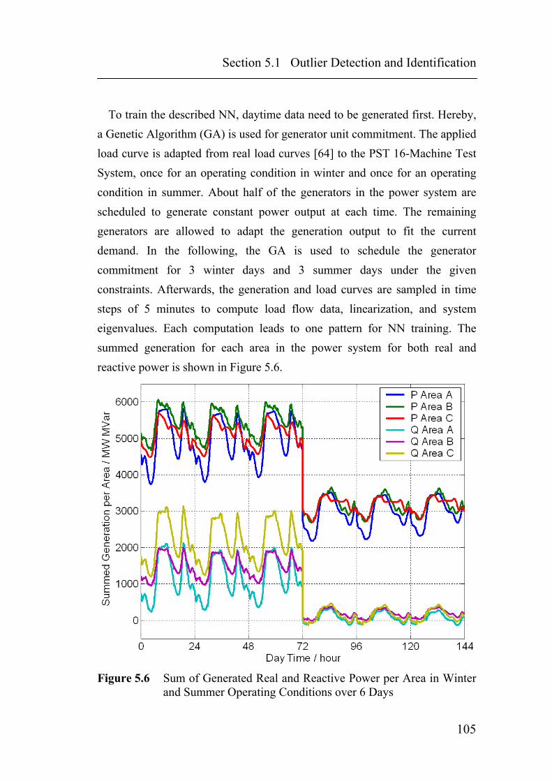
Section 5.1 Outlier Detection and Identification
To train the described NN, daytime data need to be generated first. Hereby, a Genetic Algorithm (GA) is used for generator unit commitment. The applied load curve is adapted from real load curves [64] to the PST 16-Machine Test System, once for an operating condition in winter and once for an operating condition in summer. About half of the generators in the power system are scheduled to generate constant power output at each time. The remaining generators are allowed to adapt the generation output to fit the current demand. In the following, the GA is used to schedule the generator commitment for 3 winter days and 3 summer days under the given constraints. Afterwards, the generation and load curves are sampled in time steps of 5 minutes to compute load flow data, linearization, and system eigenvalues. Each computation leads to one pattern for NN training. The summed generation for each area in the power system for both real and reactive power is shown in Figure 5.6.
Figure 5.6 Sum of Generated Real and Reactive Power per Area in Winter
and Summer Operating Conditions over 6 Days
105

Chapter 5 Robustness
The NN is trained with time series data from the database. When the NN is used on-line, the NN outputs are compared to the measured features and those showing differences beyond a certain limit are flagged as outliers. The advantage of this method results from its multidimensional characteristic. Both the history of all features (time series) and the load flow conditions are considered and thus the NN is able to predict the correct reference value to check the measurements. Figure 5.7 shows the NN results of feature forecasting for the real power on the transmission line between Area A and Area B (Feature #12 in DT-50), which is the same feature as in previous examples.
Figure 5.7 Multidimensional Feature Forecasting by NN over 6 Days for
the Real Power on a Transmission Line The figure shows the comparison between the NN target and output (top
figure) and the error as difference between the NN target and output (bottom
106

Section 5.1 Outlier Detection and Identification
figure). The NN training is carried out with a time series over 6 days. The NN inputs are 4 history data (each as a weighted average over 50 time steps back) for each input from selection DT-50, which results in a total input number of 200. Another example is given in Figure 5.8 showing the NN results for the voltage at a 400 kV bus in Area C (Feature #4 in KM-10), which is the same feature as in previous examples. The NN inputs are 4 history data (each as a weighted average over 50 time steps back) for each input from selection KM-10, which results in a total input number of 40.
Figure 5.8 Multidimensional Feature Forecasting by NN over 6 Days for a
Bus Voltage Both figures show highly accurate prediction results. Therefore, the NN
outputs can be compared to real-time measurements in order to detect bad data. However, when the features show a high deviation within very few time steps.
107

Chapter 5 Robustness
5.2 Outlier Restoration
The outlier restoration method is implemented as non-linear sequential quadratic optimization algorithm using a cost function based on an NN auto encoder. This special type of NN is trained to recognize the load flow scenarios included in the database. When used for outlier restoration, the optimization algorithm minimizes the NN auto encoder error for a given load flow scenario with bad or missing data.
5.2.1 NN Auto Encoder
The auto encoder network is a well-known type of NN and discussed in detail in [45]. This NN, shown in Figure 5.9, replicates the input vector at the output. In other words, the NN is trained to obtain identical input and output.
Figure 5.9 NN Auto Encoder
The error between input and output vector is low for any trained load flow
condition. When a new pattern contains bad data, the features of this pattern do not belong to a feasible load flow condition. Hence, the error is high when presented to the NN auto encoder. Therefore, abnormal differences between inputs and outputs of the auto encoder indicate patterns that are greatly
108

Section 5.2 Outlier Restoration
suspicious to containing bad data. The auto encoder is highly sensitive to outlier patterns. However, it is not possible to determine the feature from the new pattern, which contains the bad data. Since all features inside the NN are cross connected, a high auto encoder error of a given feature does not necessarily mean bad data. Therefore, the NN auto encoder can only be used, such as principal component residuals, to detect outlier patterns, but not outlier features.
5.2.2 Restoration Algorithm
Once a new input pattern is recognized as outlier pattern and the particular bad features are identified, the bad data have to be restored. This is possible using the same NN auto encoder network as described in the previous section. Hereby, the NN auto encoder is involved into an optimization loop where it describes the power-flow-conform relationship between the features. A sequential quadratic optimization, which is the most favorable algorithm for continuous problems, is utilized to adjust the elements of the feature vector. The algorithm restores the bad data elements by minimizing the error of the NN auto encoder.
Usually it can be assumed that most of the original measurements are correct and thus these variables can be kept constant. Hence, only some suspicious inputs need to be changed by the optimization. The restoration of bad features succeeds when the difference between the input and output vectors of the auto encoder is small. The optimization diagram is shown in Figure 5.10.
109

Chapter 5 Robustness
ConstantFeatures
VariableFeatures
Error
Target
-
Optimization
Figure 5.10 Non-linear sequential quadratic Optimization Procedure for
Feature Restoration using NN Auto Encoder The two examples given in the previous sections are used. The optimization
algorithm is applied to restore those features to their original values. In both examples, the optimization adjusts the feature determined as missing. The remaining inputs are kept constant to determine the operating point to be restored. Starting from 0 as the initial value, the optimization restores the original value within a few seconds and with high precision. Table 5.1 shows the comparison of the original feature values and the restoration results.
Example Selection Feature # Original Restored
1 DT-50 12 947.86 MW 952.56 MW
2 KM-10 4 414.75 kV 414.88 kV
Table 5.1 Restoration Results for two given Examples
110

Section 5.2 Outlier Restoration
To test the ability of the optimization algorithm to restore more than one missing input, 8 voltage features from a set of 50 inputs (DT-50) are determined as “missing”. Figure 5.11 shows the progress of restoration of selected voltages as a function of the number of function calls during the optimization process.
Figure 5.11 Progress of Feature Restoration for 8 Voltage Features
The total number of iterations is 33, which is much smaller than the total
number of calls since the optimization calls the cost function several times during each iteration step. The comparison between original and restored feature values is listed in Table 5.2. As can be seen, the restoration is very accurate.
111

Chapter 5 Robustness
Feature # Original Restored Difference
29 402.96 402.88 0.02 %
30 404.88 404.79 –0.02 %
31 227.92 227.95 0.01 %
32 383.04 382.65 –0.10 %
33 399.74 399.33 –0.10 %
34 228.92 228.02 –0.39 %
35 232.01 231.05 –0.42 %
36 414.97 414.52 –0.11 %
Table 5.2 Comparison of 8 Original and Restored Voltage Features in kV
from a total Set of 50 Inputs (DT-50) The examples shown above are representative of optimization based
restoration. Because the NN auto encoder is trained with various load flow scenarios, it always finds a solution that meets a feasible load flow condition, when the fixed variables are enough to represent this load flow situation. However, it requires that the input feature vector contains redundancy not only for a few variables, but for the whole vector. This issue can be considered in the feature selection process. When a small and large set of selected features both show low errors in OSA, the large set is preferred to be chosen since it contains definitely more redundancy than the small one. For a few missing features, the algorithm always finds the correct solution. In the investigated PST 16-Machine Test System, even for 50% missing data of 50 inputs, the algorithm is able to find a solution, which is still close enough to the real scenario to use for OSA.
112

Section 5.3 Conclusion
5.3 Conclusion
A robust OSA can be carried out based on properly designed and trained CI methods. The proposed methods for OSA allow considering different load flow conditions resulting from seasonal and topological changes. However, robust assessment requires reliable input data. This chapter discussed different methods for detection of erroneous features. The most powerful methods are the principal component residuals based method and the NN auto encoder. These methods recognize a pattern even in the case of small errors. The disadvantage is that both methods cannot detect the element in the feature vector, which is the outlier. However, the time series analysis by multidimensional feature forecasting is highly applicable because the feature prediction shows low errors and high accuracy. Comparing predicted and measured features, the elements including bad data can be identified easily. Once the outliers are detected, they can be restored by the NN auto encoder. Essential for the success of the OSA is an amount of sufficient redundancy in the selected features that allows bad data detection and restoration.
113

Chapter 5 Robustness
114

Chapter 6
Counter Measures
The previous chapters discussed the issues of oscillatory stability in large interconnected power systems, and solutions for on-line OSA using CI techniques. These techniques allow fast and accurate assessment of the current system state, and provide helpful information for the TSO who runs the power system. In the case of a critical situation, the TSO needs to know how to prevent the system from collapse and which action will lead to a better-damped power system. This information cannot be provided by OSA methods since they are designed for assessment only.
The research area of counter measures deals with the problem, which
operator action will have a stability improving impact on the power system. Of course, the system operator is trained to manage critical situations, but with the increasing complexity of the power systems, especially in Europe, the operator’s decision requires more and more technical tools.
In this chapter, a new method is proposed. It is composed of NNs and non-
linear optimization to estimate the best counter measures. The optimization algorithm maximizes the system damping, which is predicted in real-time by the OSA. Starting from a given insufficient damped initial condition in the power system, the optimization algorithm adjusts the feature vector in order to maximize the predicted system damping. A second NN is used to ensure the physical feasibility of the resulting power flow condition.
115

Chapter 6 Counter Measures
The optimization results in a new power flow feature vector, which corresponds to a situation with higher damping than the current one. The result provides the with TSO important information about stability-improving actions.
However, after the computation of counter measures, the technique is tested
in the PST 16-Machine Test System. The load flow in the power system is adjusted by a generalized OPF to the new power flow vector given by the counter measure computation. When the power system operates exactly at the operating point determined in the new power flow vector, the stability situation is expected to be improved. Therefore, the eigenvalues are computed for both the initial insufficient damped situation as well as for the new proposed operating condition after the TSO has run the suggested action. It can be shown that the system damping can be improved significantly depending on the degree of freedom of allowed actions in the power system.
116

Section 6.1 Counter Measure Computation
6.1 Counter Measure Computation
When the TSO runs the power system, there are a few items to be considered, which limit the possibilities of actions. The TSO controls the power system, but actions are limited to a set of a few control variables. Because of contractual constraints, the TSO may not be able change the generated power at particular power plants. By setting the transformer taps, the TSO can adjust the voltage level and control the power flow through transmission lines. Moreover, the generated reactive power can also be influenced.
6.1.1 Feature Classification
The features in the power system are described by 3 main characteristics, which are constant features, dependent features, and independent features. Constant features cannot be changed by the TSO such as generated power and loads, which are kept constant during the TSO’s actions. Dependent features also cannot be changed directly by the TSO, but they change depending on indirect TSO action in the power system. These features include real and reactive power flows on transmission lines, voltage angles, and bus voltages. Finally, the independent features such as transformer tap positions and generated reactive power can be changed by the TSO directly. The features classified are shown in Table 6.1.
Group 1 (Constant)
Group 2 (Independent)
Group 3 (Dependent)
Generated Real Power Generated Reactive Power Transmitted Power
Gen. Units in Operation Transformer Tap Positions Bus Voltages
Demand Voltage Angles
Table 6.1 Feature Classification according to their Characteristics
117

Chapter 6 Counter Measures
6.1.2 Control Variables
Control variables are those features in the power system that are directly controlled by the TSO. However, when the counter measure method is implemented, it is based on the feature vector selected for CI. But the feature vector contains only a few of those features, which are considered independent. Moreover, the feature vector does not include the transformer tap positions. For this reason, the control variables used in the counter measure computation are not only the independent features, but also the bus voltages. Bus voltages are controlled by transformer tap positions and therefore indirectly independent.
6.1.3 Power System Damping Maximization
The calculation of counter measures is implemented as non-linear sequential quadratic optimization algorithm using the proposed Neural Networks as cost and constraint function. The cost function performs classification and eigenvalue region prediction to determine the minimum-damping for the current system state. The minimum-damping coefficient is then maximized by the optimization algorithm under the constraint of a feasible load flow condition.
The cost function implements the NN described in Subsection 4.1.3.2. The
NN has 50 inputs based on DT-50. This NN is used for classification to give a first estimation of the operating condition. When the condition is insufficiently damped, the input is presented to the 5 NNs, shown in Subsection 4.1.5, to perform the eigenvalue region prediction. The cost function output is the minimum-damping of the predicted eigenvalue regions. It is not possible, to use the DT method in the form of a regression tree instead of the NN method. The DT method estimates directly the minimum-damping and seems therefore on first sight more applicable than the NN
118
Section 6.1 Counter Measure Computation
method. The reason is that the DT method is not a continuous model, but a non-linear sequential quadratic optimization requires a continuous cost function to be optimized. However, when using NN, the cost function output is continuous over the entire feature space.
The constraint function implements the NN auto encoder as introduced in
Subsection 5.2.1 to ensure a feasible load flow condition for the optimization result. Similarly to the feature restoration algorithm, the error as the difference between inputs and outputs of the NN auto encoder is used as indicator for the feasibility of the load flow. The smaller the error, the more likely is the load flow to a feasible situation.
During the entire optimization process, the features from Group 1 in Table
6.1 are kept constant. The control variables are the independent features from Group 2 and the bus voltages from Group 3. They are variable and therefore adjusted by the optimization algorithm in order to improve the predicted system damping. The dependent features from Group 3 except the bus voltages are adapted to a feasible load flow condition depending on the independent features using the NN auto encoder. The optimization block diagram is shown in Figure 6.1.
119

Chapter 6 Counter Measures
ConstantFeatures
VariableFeatures
Error
Target
-
OptimizationConstraint
Damping
Dependent Features
NN Auto Encoderfor Load Flow
Estimation
NN forDamping
Estimation
Figure 6.1 Non-linear sequential quadratic Optimization Procedure for
Power System Damping Maximization It is worth mentioning that the optimization results depend highly on the
chosen optimization parameters. There exists not only one unique solution, but also many possible load flow conditions, which are stable and possible to reach from the initial starting condition. Moreover, sequential quadratic algorithms may only give local solutions.
However, the result of the optimization is a vector containing the new
feature values for all dependent and independent features. Once the power system load flow is adjusted to the new operating point, the system damping increases to the optimized damping values.
An example is given in Figure 6.2 showing one dominant eigenvalue of the
PST 16-Machine Test System for a winter load flow scenario. The scenario is characterized by a real power transit of 524 MW from Area B to Area C. The figure also shows the predicted eigenvalue region constructed by NN based OSA. As can be seen in the figure, the situation is insufficiently damped. Therefore, the counter measures are computed for this situation as described
120

Section 6.1 Counter Measure Computation
in the previous section. Hereby, the 50 input features are classified into constant features, dependent features, and control variables. However, the used selection DT-50 includes 3 constant features, 39 dependent features, and 8 control variables. The 8 control variables are adjusted during the optimization process and the 39 dependent features are adjusted by the NN auto encoder in order to keep the load flow feasible.
4% 3% 2% 1% 0% -1%
Figure 6.2 Dominant Eigenvalue and Predicted Eigenvalue Region for insufficiently damped Load Flow Scenario
121

Chapter 6 Counter Measures
6.2 Realization in the Power System
In the next step, the counter measure computation results are transferred into the power system. While the counter measure optimization is based on the feature vector including only a small set of control variables, the TSO has much more control variables in the real power system that can be changed. Since there is no need to use only those control variables, which are included in the counter measure computation, the TSO may adjust all control variables in the power system. This includes all transformer tap positions and the generated reactive power at all generators.
For realization, this study uses a generalized OPF to reach the new
operating point in the power system. The realization results show the damping improvement and also provide the TSO with more system information in addition to the resulting feature vector from the counter measure computation.
Commonly, OPFs for load flow computations are based on a target function
to minimize the power system losses. However, in this case, a generalized OPF is developed for minimizing a target function defined as the difference between the desired features resulting from the counter measure computation and the actual load flow. When the new feature values are approached in the system, it will result in damping improvement. However, the generalized OPF can change not only those control variables, which are used for the counter measure computation, but all control variables available to the TSO.
It is assumed that the generated real power is subjected to be constant because of the unbundling between power transmission utilities and power generation utilities. Moreover, the power generation depends on demand and power generation contracts and the TSO is not allowed to change the contractual conditions unless the system is in the emergency state.
122

Section 6.2 Realization in the Power System
The example for counter measure estimation is based on the scenario given in Figure 6.2. The dominant eigenvalues for the scenario after the estimated counter measures are taken are shown in Figure 6.3. The initial location, before counter measures are computed, is plotted in the figure as well. Compared to the original scenario, the eigenvalue has shifted slightly and thus the system damping has improved, but marginally.
4% 3% 2% 1% 0% -1%
Figure 6.3 Computed Eigenvalues according to the proposed Counter Measures (OPF Control Variables: Transformers and Generator Voltages) and Original Dominant Eigenvalue
Because the improvement is not sufficient enough, the TSO may consider
more control actions to influence the power system. Since the inter-area oscillations are mainly caused by a large power transit between Area B and Area C, the generated real power (and thus the power exchange between these areas) should be considered as controlled variables by the OPF. Therefore, the
123

Chapter 6 Counter Measures
generated power of two selected generators are also included in the set of control variables. One generator is located in Area B and the other one in Area C. Both are close to the area-connecting tie line. The results are shown in Figure 6.4.
4% 3% 2% 1% 0% -1%
Figure 6.4 Computed Eigenvalues according to the proposed Counter Measures (OPF Control Variables: Transformers, Generator Voltages, and Generated Real Power at two Generators) and Original Dominant Eigenvalue
The figure shows much more improvement in terms of system damping
than the case in Figure 6.3. This result leads to the conclusion, that the changes of transformer tap ratios and reactive power are not sufficient in the given example to reach a well-damped system state. But when some selected real power sources are taken into account, the improvement can be enormous. To demonstrate the impact of real power transits on the system stability, the
124

Section 6.2 Realization in the Power System
real power outputs of all generators are control variables and therefore variable in the generalized OPF. However, the resulting load flow scenario shown in Figure 6.5 leads to the highest system damping when compared to the previous figures.
%
Figure 6.5 ComputMeasureVoltage
4% 3% 2% 1% 0% -1
ed Eigenvalues according to the proposed Counter s (OPF Control Variables: Transformers, Generator
s, and Generated Real Power)
125

Chapter 6 Counter Measures
6.3 Conclusion
This chapter introduced a new method for counter measure computation, which is directly based on the OSA tools proposed within this study. The features leading to improvement in system damping are calculated within an optimization. The power flow conditions are considered by an NN auto encoder and the expected system damping is assessed by the NN based OSA tool developed in Chapter 4. This method is fast and can be implemented as additional on-line tool for TSOs. The optimization result is a vector with new feature values providing the TSO with information about a better-damped system state. To reach the desired power flow, the TSO can take different control actions that are not considered in the previous feature calculation. This includes the change in the transformer tap positions. As a powerful tool, it is suggested to use a generalized OPF where the target function is defined as the difference between the desired features resulting from the counter measure computation and the actual load flow. This OPF can consider all control actions available to the TSO.
To achieve considerable damping improvement, it may be necessary to
change the real power flow between areas swinging against each other. In the test system used in this study, control variables concerning mainly voltages and reactive power resulted in marginal improvements. By allowing the real power generation in different areas to change, the generalized OPF was able to estimate a new power flow with noticeably better system damping.
126

Chapter 7
Conclusion
The European power system has grown very fast in a short period of time and it is expected to be extended even more in the near future. These extensive interconnections alter the stable operating region of the system, and the power network experiences inter-area oscillations. Moreover, the deregulation of electricity markets in Europe also impacted negatively on the stability of the power system.
When the complete power system model is available, it is recommended to
perform the OSA analytically by system linearization and eigenvalue computation. But this is usually not applicable for on-line OSA since the system modeling requires detailed knowledge about the complete dynamic system data and operation settings. The computations are time-consuming and require expert knowledge.
Therefore, the main focus of this PhD Dissertation was the development of
new tools based on CI applications such as NNs, NF, and DTs for fast on-line OSA. Since CI methods are based only on a small set of data they do not require the complete system model and the CI outputs are directly related to the stability problem. CI methods are learned on training patterns and show good performance in interpolation. Moreover, CI applications are fast and can therefore be used as on-line tools for TSOs. Because they need only a small set of system information, they are highly recommended in Europe’s competitive energy market.
127

Chapter 7 Conclusion
Before CI methods are trained, the training data must be generated first. Therefore, the dynamic PST 16-Machine Test System was developed. The test system is designed as a dynamic model of a large-scaled power system. It was used to run various load flow computations under different operating points to generate the necessary CI training data. The used OPF ensures the generation of feasible training data within typical operating limits of modern power systems. The computed eigenvalues are used as targets during the CI training and for error evaluation afterwards to verify the quality of the eigenvalue prediction by CI.
Once the complete power system data are generated in the test system, different CI methods are trained on the data for OSA. All applied techniques, NNs, DTs, and NF show accurate results. As shown in Chapter 4, the applied CI methods can be implemented in various approaches for proper OSA. The power system state can be classified, the minimum-damping can be estimated or eigenvalue coordinates can be predicted directly. The CI methods also can be designed to classify fixed geometric eigenvalue regions or predict variable eigenvalue regions.
However, all CI methods show a different training behavior. NN and NF methods are continuous models, but they require long training times. In the contrary, DTs are grown within seconds. But they can only be designed as single-output models. The lack is compensated, when multiple DTs are grown parallel as shown in Subsection 4.3.4 to predict eigenvalue regions.
Within this PhD Dissertation, different selection approaches for the CI
input features are introduced and discussed. They are based on both conventional computational methods such as PCA and k-Means clustering, and on CI methods such as DT and GA. Clustering is a common technique to find structural similarities in data. It is applied in this study together with the PCA, which is used to reduce the data to a small set that can be clustered easily. However, the process of clustering is not related to the eigenvalues and
128

the OSA methods, and therefore, it finds only similar inputs. The final selection is performed by engineering judgment in order to select not features in the cluster centers, but features, mostly related to the OSA problem. Another selection is proposed by the use of DTs because they are grown on both input and target data. Therefore, knowledge about the OSA problem is included in the tree structure. Branch nodes on the top part of the tree provide information, which features show the best performance in the data separability. Therefore, those features result in a proper selection of OSA inputs. However, a third approach considers a GA to select input features based on a cost function. This cost function involves a DT for OSA and the prediction error is a measure for the quality of the selected inputs.
Changes in the network topology, the load situation, the operating point,
and the influence of bad and missing data affect the quality and reliability of the proposed OSA methods. Therefore, the issues of robustness are discussed and methods for bad data detection and restoration are developed. On one side, statistical methods such as the principal component residuals and similarity analysis based on the correlation coefficient are applied. The principal component residuals show highly accurate results detecting bad data on a newly presented input pattern, but this method cannot detect the element containing the bad data. The similarity analysis can detect the element, but the detection success depends highly on the situation, e.g. the badness of the element and on the number of outliers. On the other side, a new proposed method including an NN is used to predict the current feature values based on the feature history data. The predicted and the measured values are compared and large differences indicate suspicious outliers. This method benefits from the information in the recorded history data, the multidimensional characteristic since all features are included in one NN, and it can identify multiple outliers easily.
129

Chapter 7 Conclusion
The outlier restoration method is implemented based on non-linear sequential quadratic optimization combined with a NN. The NN is trained to recognize the load flow scenarios included in the database. During the outlier restoration process, the optimization algorithm adjusts the values of the features containing bad data until the complete pattern matches a feasible load flow condition.
However, in the case of a critical situation, the TSO also would like to
know how to prevent the system from collapse and which action will lead to a better-damped power system. Therefore, a new tool for counter measure computation is proposed. This tool is based on the OSA methods developed within this PhD Dissertation and provides the TSO with information, which operator action will have a stability improving impact on the power system. The counter measures are computed by non-linear sequential quadratic optimization similar to the bad data restoration process. After the optimization, the results are verified in the power system operated at the new proposed operating point.
130

Appendix
Appendix
A.1 The 16-Machine Dynamic Test System The PST 16-Machine Test System used in this study is a newly developed
dynamic test system. The main focus of this system is on the power system dynamics and inter-area oscillations in the time range of a few seconds to minutes [65]. The PST 16-Machine Test System is modeled by using real data from new generators and controllers for different units. The power system operates with 3 different types of generators, such as hydro power generators, thermal driven generators, and nuclear driven generators. For hydro generators, the rated generator power is 220 MW per block. For thermal driven generators, the block size is 247 MW, and for nuclear driven generators about 259 MW. However, a power plant in the network is modeled by connecting a particular number of generator units to the electric transmission system. The generator models are 5th order and the exciter models are obtained from IEEE standard types [19]. Hereby, the hydro generators are controlled by a slightly modified version of the ST1A excitation system. The thermal driven generators use the DC1A exciter model, and the nuclear driven generators use the AC1A exciter model. The system consists of 3 strongly meshed areas. Each has 5 – 6 generators. Partly weak transmission lines connect these areas. The transmission lines are weak because of their distance of about 290 km. Thus, inter-area oscillations can occur, especially when power is transmitted over these area connections.
However, the system is designed for power exchange between these areas. The first area (Area A) contains mostly hydro power plants and is considered to be a power exporting area. Area B and area C are load demanding areas that import power from area A. The total generation of the system is about 16 GW and the different voltage level cover the 380 kV, 220 kV, and the 110 kV level.
131

132
14630
MV
A
630
MV
A
78
250
MV
A
1
2x24
7 M
VA
6
4
2
4x24
7 M
VA
AR
EA C
6x24
7 M
VA
1312
5x24
7 M
VA
6x24
7 M
VA
3
4
1
7
5
16
17
300
MV
A
DL
50 k
mD
L10
0 km
11
10
9
10
800
MV
A
7
5a
6
8
1511
4x24
7M
VA
31
4
6x25
9 M
VA
AR
EA B
2x63
0 M
VA
630
MV
A
4x25
9 M
VA
56
DL
290
km
5x25
9 M
VA
4x63
0 M
VA 9
4x24
7 M
VA
2
AR
EA A
23
18
19
250
MV
A
2x25
0 M
VA
380
kV22
0 kV
110
kV15
.75
kVD
L10
0 km
100
km
100
km
DL
290
km50
km
DL
80 k
m
50 k
m
50 k
m
DL
80 k
m DL
70 k
mD
L50
km D
L50
km
90 k
m 70 k
m
DL
70 k
m
DL
40 k
m
20 k
m
20 k
m20
km
80 k
m
30 k
m20
km
DL
290
km
DL
20 k
mD
L 40
km
DL
40km
40 k
m40 k
m 40 k
m
DL
50 k
m
50 k
m40 k
m
40 k
m
40 k
m
60 k
m100
km 40 k
m40
km
50 k
m100
km
50 k
m
DL
40 k
m
DL
70 k
m
DL
50 k
m
5x25
9 M
VA
250
MV
A
100
km
100
m
5x22
0M
VA
5x22
0M
VA
2x22
0M
VA
250
MV
A
DL
30 k
m
DL
30 k
m
~
~
~~
~~
~
5b
~
~~
~
~
~
~ ~
~
5x22
0M
VA
5x22
0M
VA
380
kV
380
kV
220
kV
220
kV
380
kV
110
kV
A.2 PST16 One-Line Diagram
Appendix

Appendix
A.3 System Topology
Buses Lines Transformers Generators
Area A 17 12 9 6
Area B 21 15 10 5
Area C 28 24 9 5
Total 66 51 28 16
A.4 Distribution of Generators
Number of Generators
Hydro Thermal Nuclear
Area A 5 1 0
Area B 0 1 4
Area C 0 5 0
A.5 Load and Generation
Load Generation
Area A 2,000 MW 4,840 MW
Area B 6,100 MW 5,641 MW
Area C 7,465 MW 5,450 MW
Total 15,565 MW 15,931 MW
133

Appendix
A.6 Operating Conditions Since the operating point in real power systems changes continually,
different operating conditions, which base on the initial system base case, need to be created. In this study, 5 different operating conditions are used. The first one is the base case, which is considered as a high load condition in winter. From this situation, a medium load case and a low load case are derived. To consider the possibility of a change in the network’s topology, two more high load conditions include switching action of lines with a high impact on the system stability. Hereby, one circuit of the area connecting double tie line from A to B is switched off in Winter S1 and one circuit of the area connecting double tie line from B to C is switched off in Winter S2. The double line between A and C is not used for switching action because the loss of one circuit results in total system instability.
# Name Description
1 Winter Base Case, Generation and Load at 100 %
2 Spring Generation and Load decreased to 80 %
3 Summer Generation and Load decreased to 60 %
4 Winter S1 One Circuit of A to B Tie Line switched off
5 Winter S2 One Circuit of B to C Tie Line switched off
A.7 Pattern Generation for CI Training To generate training data for the CI methods, different load flow scenarios
under varying operating conditions are considered. These scenarios are generated by real power transmission between 2 areas at a time. To archive this real power exchange, the total generation in one area is increased while the total power in the other area is decreased. When the total generation in one area is changed, the change is distributed equally among all the generators in
134

Appendix
this area. However, since power plants in the network are modeled by connecting a particular number of generator units to the network, the number can be adapted to the generator condition. Thus, if the generated power of a power plant falls below the minimum number of blocks necessary to generate the required output power, one unit is disconnected. The model also allows additional generating units to be connected when the demand increases. The different load flow scenarios result in generating 5,360 patterns.
135

Appendix
136
References
References [1] UCTE, Annual Report 2002, available:
http://www.ucte.org/publications/library/e_default_2002.asp [2] UCTE, Annual Report 2003, available:
http://www.ucte.org/publications/library/e_default_2003.asp [3] UCTE, System Adequacy Forecast 2004 - 2010 Report, available:
http://www.ucte.org/publications/library/e_default_2004.asp [4] U. Bachmann, I. Erlich and E. Grebe, “Analysis of interarea oscillations
in the European electric power system in synchronous parallel operation with the Central-European networks”, IEEE PowerTech, Budapest, 1999
[5] H. Breulmann, E. Grebe, et al., “Analysis and Damping of Inter-Area
Oscillations in the UCTE/CENTREL Power System”, CIGRE 38-113, Session 2000
[6] K. Küßner, I. Erlich, H.H. Wilfert, “Design of Inter-Area Oscillations
Damping Controllers using Global Measurements”, IEEE Porto Power Tech Conference, Portugal, September 2001
[7] C.A. Canizares, et al., “Linear Performance Indices to Predict
Oscillatory Stability Problems in Power Systems”, IEEE Trans. on Power Systems, vol. 19, no. 2, May 2004
[8] X.Y. Wen, V. Ajjapu, “Novel Computational Techniques for Power
System Oscillatory Stability Assessment”, Conference Proceedings IREP Symposium, Italy, August 2004
137

References
[9] L. Wang, C.Y. Chung, “Increasing Power Transfer Limits at Interfaces constrained by Small-Signal Stability”, PES Winter Meeting, IEEE vol. 2, pp. 1184-1187, January 2002
[10] N. Martins, S. Gomes Jr., et al., “Some Recent Developments in Small-
Signal Stability and Control”, PES Winter Meeting, IEEE vol. 2, pp. 1171-1177, January 2002
[11] M.J. Gibbhard, N. Martins, et al., “Recent Applications of Linear
Analysis Techniques”, IEEE Trans. on Power Systems, vol. 16, no. 1, February 2001
[12] L.J. Cai, I. Erlich, “Coordination between Transient and Damping
Controller for Series Facts Devices using Anfis Technology”, Conference Proceedings IFAC 2003, Seoul, Korea, September 2003
[13] M.A. El-Sharkawi, “Neural network and its ancillary techniques as
applied to power systems”, IEE Colloquium on Artificial Intelligence Applications in Power Systems, pp. 3/1 - 3/6, 1995
[14] Y. Mansour, E. Vaahedi, M.A. El-Sharkawi, “Large Scale Dynamic
Security Screening and Ranking using Neural Networks”, IEEE Trans. on Power Systems, vol. 12, no. 2, May 1997
[15] G.T. Heydt, C.C. Liu, et al., “Solutions for the Crisis in Electric Power
Supply”, IEEE Computer Applications in Power, July 2001 [16] C. Rehtanz, Autonomous Systems and Intelligent Agents in Power
System Control and Operation, Berlin, Springer, 2003 [17] O. Nelles, Nonlinear System Identification, Springer, Berlin, 2001
138

References
[18] P. Kundur, J. Paserba, et al., “Definition and Classification of Power System Stability”, IEEE Trans. on Power Systems, vol. 19, no. 3, pp. 1387-1401, August 2004
[19] P. Kundur, Power System Stability and Control, McGraw-Hill, New
York, 1994 [20] M. Kurth, E. Welfonder, “Oscillation Behaviour of the Enlarged
European Power System under Deregulated Energy Market Conditions”, IFAC 2003, Seoul, Korea, September 15-18, 2003
[21] S.P. Teeuwsen, Assessment of the Small Signal Stability of
Interconnected Electric Power Systems under Stressed Load Flow Conditions by the Use of Artificial Neural Networks, Diploma Thesis, unpublished, Gerhard-Mercator Universität, Duisburg, July 2001
[22] S.P. Teeuwsen, A. Fischer, I. Erlich, M.A. El-Sharkawi, “Assessment of
the Small Signal Stability of the European Interconnected Electric Power System Using Neural Networks”, Conference Proceedings LESCOPE 2001, Halifax, Canada, July 2001
[23] S.P. Teeuwsen, I. Erlich, M.A. El-Sharkawi, “Feature Reduction for
Neural Network based Small-Signal Stability Assessment”, Conference Proceedings PSCC 2002, Sevilla, Spain, June 2002
[24] L.A. Wehenkel, Automatic Learning Techniques in Power Systems,
Kluwer Academic Publishers, Boston, 1998 [25] M. Mendel, K.S. Fu, Adaptive, learning and pattern recognition
systems: theory and applications, New York, Academic Press, 1972
139

References
[26] M.B. Zayan, M.A. El-Sharkawi, N.R. Prasad, “Comparative Study of Feature Extraction Techniques for Neural Network Classifier”, International Conference on Intelligent Systems Applications to Power Systems, ISAP’96, pp. 400-404, 1996
[27] C.A. Jensen, M.A. El-Sharkawi, R.J. Marks II, “Power System Security
Assessment using Neural Networks: Feature Selection using Fisher Discrimination”, IEEE Trans. on Power Systems, vol. 16, no. 4, November 2001
[28] I.N. Kassabalidis, M.A. El-Sharkawi, et al., “Dynamic Security Border
Identification using Enhanced Particle Swarm Optimization”, IEEE Trans. on Power Systems, vol. 17, no. 3, August 2002
[29] L.S. Moulin, M.A. El-Sharkawi, R.J. Marks, A.P. Alves da Silva,
“Automatic Feature Extraction for Neural Network Based Power Systems Dynamic Security Evaluation”, ISAP 2001, no. 21, Budapest, Hungary, June 2001
[30] R.O. Duda, et al., Pattern Classification, New York, Wiley, 2001 [31] I.T. Jolliffe, Principal Component Analysis, Springer, New York, 1986 [32] Visual Numerics, IMSL Fortran 90 MP Library Help, Stat/Library,
Volume 2, Chapter 11, Cluster Analysis [33] Breiman, et al., Classification and Regression Trees, Wadsworth Int.,
Calif., 1984 [34] R. Jang, Neuro-Fuzzy and Soft Computing, Prentice Hall, NJ, 1997 [35] J.R. Quinlan, “Induction of Decision Trees,” Machine Learn., vol. 1, pp.
81-106, 1986
140

References
[36] J.R. Quinlan, C4.5 Programs for Machine Learning, Morgan Kaufmann Publishers, San Mateo, Calif., 1993
[37] C. Huang, J.R.G. Townshend, “A stepwise regression tree for nonlinear
approximation: applications to estimating subpixel land cover”, International Journal of Remote Sensing, vol. 24, no. 1, 75-90, 2003
[38] H. Kim, G.J. Koehler, “Theory and Practice of Decision Tree
Induction”, Omega, Vol. 23, No. 6, pp.637-652, 1995 [39] K.F. Man, K.S. Tang, S. Kwong, Genetic Algorithms, Springer, London,
1999 [40] L.J. Cai, Robust Coordinated Control of FACTS Devices in Large
Power Systems, Ph.D. Thesis, University of Duisburg-Essen, February 2004
[41] M.A. El-Sharkawi and S.J. Huang, “Ancillary technique for neural
network applications”, IEEE Int. Conf. Neural Networks, Orlando, FL, pp. 3724-3729, June 1994
[42] M.A. El-Sharkawi, “Neural Networks’ Power”, IEEE Potentials, vol.
15, no. 5, pp. 12-15, December 1996, January 1997 [43] Y. Mansour, E. Vaahedi, M.A. El-Sharkawi, “Dynamic security
contingency screening and ranking using neural networks”, IEEE Trans. on Neural Networks, vol. 8, no. 4, pp. 942-950, July 1997
[44] Fuzzy Logic Toolbox – For Use with Matlab, The Mathworks Inc., 1999 [45] R.D. Reed and R.J. Marks II, Neural Smithing, MIT Press, Cambridge,
Mass., 1999
141

References
[46] S.S. Haykin, Neural Networks: A Comprehensive Foundation, Prentice Hall, London, 1999
[47] Neural Network Toolbox – For Use with Matlab, The Mathworks Inc.,
2001 [48] C.M. Bishop, Neural Networks for Pattern Recognition, Clarendon
Press, Oxford, 1996 [49] R. Fullér, Introduction to Neuro-Fuzzy Systems, Pysica-Verlag,
Heidelberg, 2000 [50] E. Czogała, J. Leski, Fuzzy and Neuro-Fuzzy Intelligent Systems,
Physica-Verlag, Heidelberg, 2000 [51] H.-H. Bothe, Neuro-Fuzzy Methoden, Springer, Berlin, 1998 [52] T. Takagi, M. Sugeno, “Fuzzy identification of systems and its
applications to modeling and control,” IEEE Trans. Syst., Man, Cybern., vol. 15, pp. 116-132, 1985
[53] E. Lughofer, “Online Adaptation of Takagi-Sugeno Fuzzy Inference
Systems”, Technical Report FLLL-TR-0217, Fuzzy Logic Laboratorium, Linz-Hagenberg
[54] E. Handschin, E. Kliokys, “Transformer Tap Position Estimation and
Bad Data Detection using Dynamic Signal Modelling”, IEEE Trans. on Power Systems, vol. 10, no. 2, May 1995
[55] J.C.S. Souza, et al., “Data Debugging for Real-Time Power System
Monitoring based on Pattern Analysis”, IEEE Trans. on Power Systems, vol. 11, no. 3, August 1996
142

References
[56] J.C.S. Souza, et al., “Online Topology Determination and Bad Data Suppression in Power Systems Operation using Artificial Neural Networks”, IEEE Trans. on Power Systems, vol. 13, no. 3, August 1998
[57] H. Salehfar, R. Zhao, “A neural network preestimation filter for bad-data
detection and identification in power system state estimation”, Electric Power Systems Research, 34, pp. 127-134, 1995
[58] P. Rousseeuw, B. van Zomeren, “Unmasking multivariate outliers and
leverage points”, Journal of the American Statistical Association, vol. 85, pp. 633-639, 1990
[59] D. Rocke, D. Woodruff, “Identification of outliers in multivariate data”,
Journal of the American Statistical Association, vol. 91, pp. 1047-1061, 1996
[60] R. Gnanadesikan, Methods for Statistical Data Analysis of Multivariate
Observations, Wiley, New York, 1997 [61] D.M. Hawkins, Identification of Outliers, Chapman and Hall, London,
1980 [62] S.J. Huang, J.M. Lin, “Enhancement of Power System Data Debugging
using GSA-Based Data-Mining Technique”, IEEE Trans. on Power Systems, vol. 17, no. 4, November 2002
[63] S. Hawkins, H.X. He, G. Williams, R. Baxter, “Outlier Detection Using
Replicator Neural Networks”, Proceedings of the 4th International Conference on Data Warehousing and Knowledge Discovery, Lecture Notes in Computer Science, vol. 2454, Springer, 2002. Pages 170-180
[64] RTE France, Transmission System Operator, Load Curves available at
http://www.rte-france.com/jsp/an/courbes/courbes.jsp
143

References
[65] S.P. Teeuwsen, I. Erlich, M.A. El-Sharkawi, “Neural Network based Classification Method for Small-Signal Stability Assessment”, IEEE PowerTech, Bologna, Italy, June 23-26, 2003
144

List of Symbols
List of Symbols Latin Symbols A State matrix (system matrix)
kka Element of the k-th state in state matrix A
a Sampling point activation act Sum of sampling point activations B Control matrix C Output matrix C Empirical covariance matrix of F D Feed-forward matrix d Distance between eigenvalue and sampling point
maxd Maximum distance between eigenvalue and sampling point
),( θxtd Local DT regression model at node t
)(tE DT error measure at node t
F Complete feature matrix of dimension np ×
remF Remaining feature matrix after residual computation )PC(F Transformed feature matrix of dimension np × )PC(
qF Reduced transformed feature matrix of dimension qp ×
f Frequency of oscillation
evf Frequency of oscillation associated with eigenvalue λ
maxregf Frequency maximum of predicted eigenvalue region
minregf Frequency minimum of predicted eigenvalue region
sf Frequency of sampling point
g Number of patterns in the subset
145

List of Symbols
DK Damping torque coefficient of a synchronous machine
SK Synchronizing torque coefficient of a synchronous machine
k Number of selected features as CI input
fk Scaling factor for imaginary part distance
σk Scaling factor for real part distance
tN Number of patterns at node in DTs t
n Number of eigenvalues, total number of features Number of patterns p
kip Participation factor for the k-th state variable and the i-th mode
q Number of principal components used for feature reduction
R Vector with scalar residuals of the residual matrix Y
R Scalar residual of a newly presented input pattern *R Limit of R for comparison with R
r Number of residuals S Subset matrix for similarity analysis of dimension ng ×
s Number of sampling points in the observation area
is Elements of the subset matrix corresponding to feature i S
T Matrix including eigenvectors of C of dimension n n×
qT Reduced matrix of eigenvectors of C of dimension n q×
rT Reduced matrix of eigenvectors of C of dimension rn ×
DT Damping torque of a synchronous machine
ST Synchronizing torque of a synchronous machine
t Index for node numbers in DTs u Vector of inputs to the system
0u Initial vector of inputs to the system
x State vector with state variables n x
0x Initial state vector
Y Residual matrix of dimension rp ×
146

List of Symbols
y Vector of outputs
z Vector of transformed state variables
Greek Symbols α Transformed feature matrix after PCA of dimension qp ×
δ∆ Rotor angle perturbation of a synchronous machine f∆ Sampling step width for frequency
regf∆ Frequency accuracy of eigenvalue region prediction
regξ∆ Damping accuracy of eigenvalue region prediction
σ∆ Sampling step width for σ
eT∆ Change in electromagnetic torque of a synchronous machine
iη Outlier factor corresponding to feature i
xiη Inlier factor of subset matrix corresponding to feature i S
θ Vector with modifiable DT regression parameters λ Eigenvalue of system matrix A
iλ Eigenvalue of A associated with the i-th mode
kλ Eigenvalue of the empirical covariance matrix C
υ Retained variability of the PCA reduction ξ Damping coefficient associated with eigenvalue λ
minξ Minimum-damping coefficient for all eigenvalues
maxregξ Damping maximum of predicted eigenvalue region
minregξ Damping minimum of predicted eigenvalue region 2Σ Diagonal variance matrix of C including variances 2
xσ
σ Real part of eigenvalue λ
evσ Real part of eigenvalue λ
147

List of Symbols
kσ Singular value of the feature matrix F
sσ Real part of sampling point 2xσ Variances of the empirical covariance matrix C
iΦ Right eigenvector associated with the i-th eigenvalue
kiΦ Right eigenvector element
φ Impurity function for classification trees
iΨ Left eigenvector associated with the i-th eigenvalue
ikΨ Left eigenvector element
ω Imaginary part of eigenvalue λ
148

List of Abbreviations
List of Abbreviations ANFIS Adaptive Neural Network based Fuzzy Inference System CENTREL Central European Power System CI Computational Intelligence DT Decision Tree FACTS Flexible AC Transmission System FIS Fuzzy Inference System GA Genetic Algorithm HVDC High-Voltage DC KM k-Means Cluster Algorithm MF Membership Function NF Neuro Fuzzy NN Neural Network OPF Optimal Power Flow OSA Oscillatory Stability Assessment PCA Principal Component Analysis PNN Probabilistic Neural Network PSS Power System Stabilizer PST 16-Machine Dynamic Test System SCV Static Var Compensator STD Standard Deviation TSO Transmission System Operator UCTE Union for the Coordination of Transmission of Electricity
149

List of Abbreviations
150

Resume
Resume Personal Data: Name Simon Patrick Teeuwsen Date of Birth May 9th, 1976 Place of Birth Krefeld, Germany Nationality Dutch Studies: 2001 – 2005 Research Assistant Institute of Electrical Power Systems University of Duisburg-Essen, Duisburg 1997 – 2001 Graduate Student Institute of Electrical Power Systems Gerhard-Mercator University, Duisburg 2000 – 2001 Visiting Graduate Dept. of Electrical Power Engineering University of Washington, Seattle, USA 1995 – 1997 Undergraduate Student Dept. of Electrical Engineering Gerhard-Mercator University, Duisburg School: 1986 – 1995 Secondary School Bischöfliche Maria Montessori Gesamtschule, Krefeld 1982 – 1986 Primary School Bischöfliche Maria Montessori Grundschule, Krefeld
151

Resume
152

Published Papers
Published Papers
Papers on Meetings and Conferences [P1] S.P. Teeuwsen, A. Fischer, I. Erlich, M.A. El-Sharkawi, “Assessment
of the Small Signal Stability of the European Interconnected Electric Power System Using Neural Networks”, LESCOPE 2001, Halifax, Canada, July 11-13, 2001
[P2] S.P. Teeuwsen, “Feature Selection for Small-Signal Stability
Assessment”, Dresdner Kreis 2002, Werningerode, Germany, March 18-20, 2002, ISBN 3-929757-52-4
[P3] S.P. Teeuwsen, I. Erlich, M.A. El-Sharkawi, “Feature Reduction for
Neural Network based Small-Signal Stability Assessment”, PSCC 2002, Sevilla, Spain, June 24-28, 2002
[P4] I. Erlich, S.P. Teeuwsen, U. Bachmann, “Schätzung der statisch
oszillatorischen Stabilität von Verbundnetzen auf der Basis von ausgewählten Prozessinformationen”, 6. GMA/ETG-Fachtagung Netzregelung, München, Germany, May 21-22, 2003
[P5] S.P. Teeuwsen, I. Erlich, M.A. El-Sharkawi, “Neural Network based
Classification Method for Small-Signal Stability Assessment”, IEEE PowerTech, Bologna, Italy, June 23-26, 2003
[P6] S.P. Teeuwsen, I. Erlich, M.A. El-Sharkawi, “Small-Signal Stability
Assessment based on Advanced Neural Network Methods”, IEEE PES General Meeting, Toronto, Canada, July 13-17, 2003
153

Published Papers
[P7] S.P. Teeuwsen, I. Erlich, M.A. El-Sharkawi, “Advanced Method for
Small-Signal Stability Assessment based on Neural Networks”, ISAP 2003, Lemnos, Greece, August 31-September 3, 2003
[P8] S.P. Teeuwsen, I. Erlich, U. Bachmann, “Small-Signal Stability
Assessment of the European Power System based on Advanced Neural Network Method”, IFAC 2003, Seoul, Korea, September 15-18, 2003
[P9] S.P. Teeuwsen, I. Erlich, M.A. El-Sharkawi, “Robust Oscillatory
Stability Assessment for Large Interconnected Power Systems”, IEEE PES General Meeting, Denver, USA, June 6-10, 2004
[P10] S.P. Teeuwsen, I. Erlich, M.A. El-Sharkawi, “Decision Tree based
Oscillatory Stability Assessment for Large Interconnected Power Systems”, PSCE 2004, New York, USA, October 10-13, 2004
154

Published Papers
Papers considered for Submission [P11] S.P. Teeuwsen, I. Erlich, M.A. El-Sharkawi, “Fast Eigenvalue
Assessment for Large Interconnected Powers Systems“, Accepted Paper, IEEE PES General Meeting, San Francisco, USA, June 12-16, 2005
[P12] S.P. Teeuwsen, I. Erlich, M.A. El-Sharkawi, “Small-Signal Stability
Assessment for large Power Systems using Computational Intelligence“, Accepted Paper, IEEE PES General Meeting, San Francisco, USA, June 12-16, 2005
[P13] S.P. Teeuwsen, I. Erlich, M.A. El-Sharkawi, “Genetic Algorithm and
Decision Tree based Oscillatory Stability Assessment”, Accepted Paper, IEEE PowerTech, St. Petersburg, Russia, June 27-30, 2005
[P14] S.P. Teeuwsen, I. Erlich, M.A. El-Sharkawi, “Methods for Estimation
of Counter Measures to Improve Oscillatory Stability in Power Systems”, Submitted to PSCC 2005, Liege, Belgium, August 22-26, 2005
[P15] S.P. Teeuwsen, L.J. Cai, I. Erlich, “Dynamic Voltage Stability
Assessment and Control by Computational Intelligence”, Submitted to ISAP 2005, Washington DC, USA, November 6-10, 2005
155