Engineering manual No. 25

Updated: 03/2018

1

Slope stability assessment

Program: FEM

File: Demo_manual_25.gmk

The objective of this manual is to analyse the slope stability degree (factor of safety) using

the Finite Element Method.

Task specification

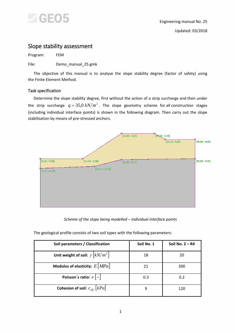
Determine the slope stability degree, first without the action of a strip surcharge and then under

the strip surcharge 20,35 mkNq . The slope geometry scheme for all construction stages

(including individual interface points) is shown in the following diagram. Then carry out the slope

stabilisation by means of pre-stressed anchors.

Scheme of the slope being modelled – individual interface points

The geological profile consists of two soil types with the following parameters:

Soil parameters / Classification Soil No. 1 Soil No. 2 – R4

Unit weight of soil: 3mkN 18 20

Modulus of elasticity: MPaE 21 300

Poisson´s ratio: 0.3 0.2

Cohesion of soil: kPaceff 9 120

2

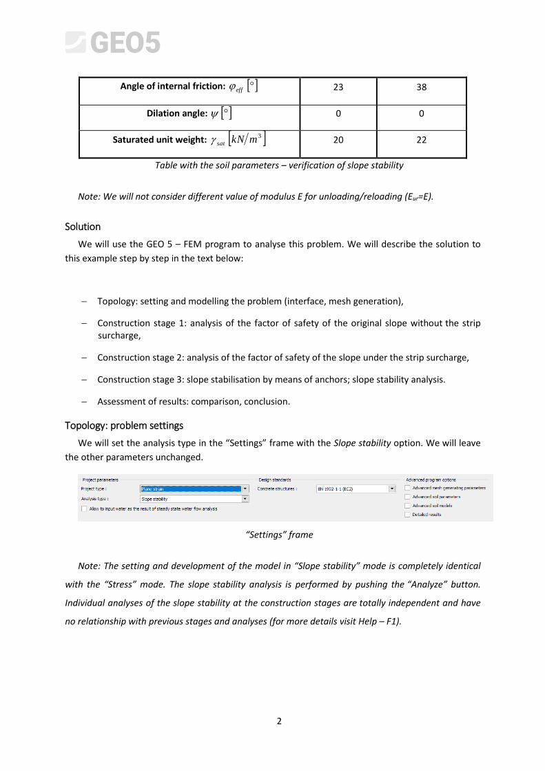
Angle of internal friction: eff 23 38

Dilation angle: 0 0

Saturated unit weight: 3mkNsat 20 22

Table with the soil parameters – verification of slope stability

Note: We will not consider different value of modulus E for unloading/reloading (Eur=E).

Solution

We will use the GEO 5 – FEM program to analyse this problem. We will describe the solution to

this example step by step in the text below:

Topology: setting and modelling the problem (interface, mesh generation),

Construction stage 1: analysis of the factor of safety of the original slope without the strip surcharge,

Construction stage 2: analysis of the factor of safety of the slope under the strip surcharge,

Construction stage 3: slope stabilisation by means of anchors; slope stability analysis.

Assessment of results: comparison, conclusion.

Topology: problem settings

We will set the analysis type in the “Settings” frame with the Slope stability option. We will leave

the other parameters unchanged.

“Settings” frame

Note: The setting and development of the model in “Slope stability” mode is completely identical

with the “Stress” mode. The slope stability analysis is performed by pushing the “Analyze” button.

Individual analyses of the slope stability at the construction stages are totally independent and have

no relationship with previous stages and analyses (for more details visit Help – F1).

3

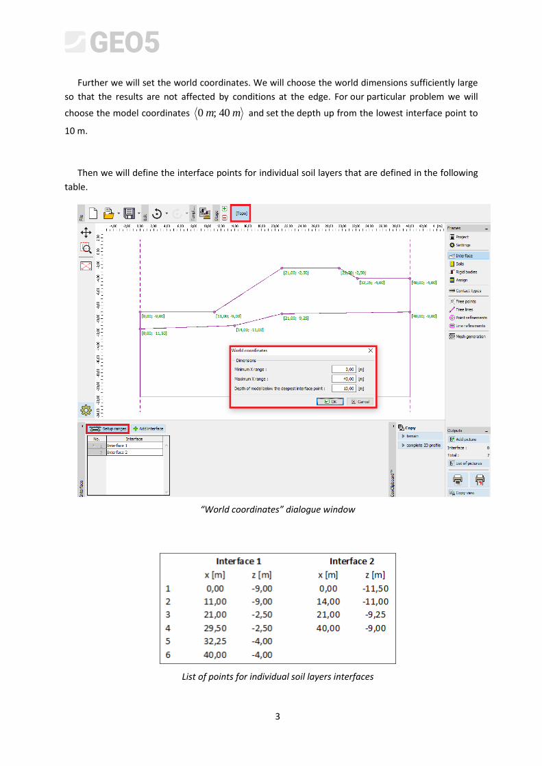
Further we will set the world coordinates. We will choose the world dimensions sufficiently large

so that the results are not affected by conditions at the edge. For our particular problem we will

choose the model coordinates mm 40;0 and set the depth up from the lowest interface point to

10 m.

Then we will define the interface points for individual soil layers that are defined in the following

table.

“World coordinates” dialogue window

List of points for individual soil layers interfaces

4

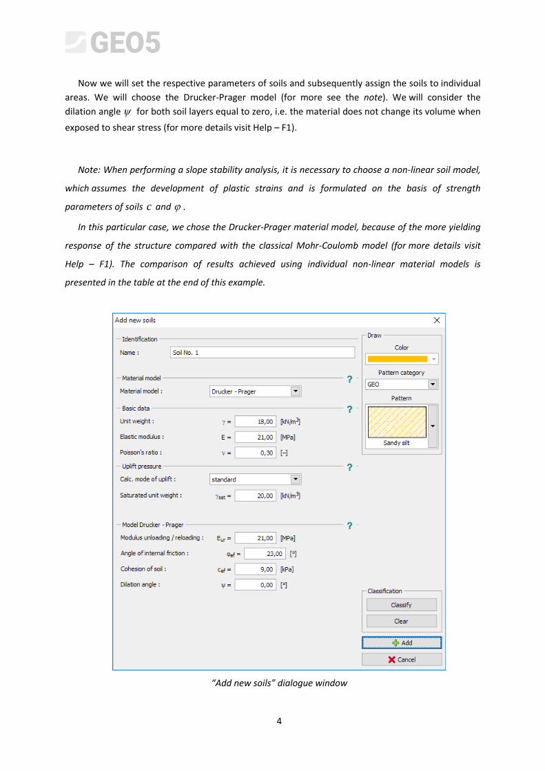
Now we will set the respective parameters of soils and subsequently assign the soils to individual

areas. We will choose the Drucker-Prager model (for more see the note). We will consider the

dilation angle for both soil layers equal to zero, i.e. the material does not change its volume when

exposed to shear stress (for more details visit Help – F1).

Note: When performing a slope stability analysis, it is necessary to choose a non-linear soil model,

which assumes the development of plastic strains and is formulated on the basis of strength

parameters of soils c and .

In this particular case, we chose the Drucker-Prager material model, because of the more yielding

response of the structure compared with the classical Mohr-Coulomb model (for more details visit

Help – F1). The comparison of results achieved using individual non-linear material models is

presented in the table at the end of this example.

“Add new soils” dialogue window

5

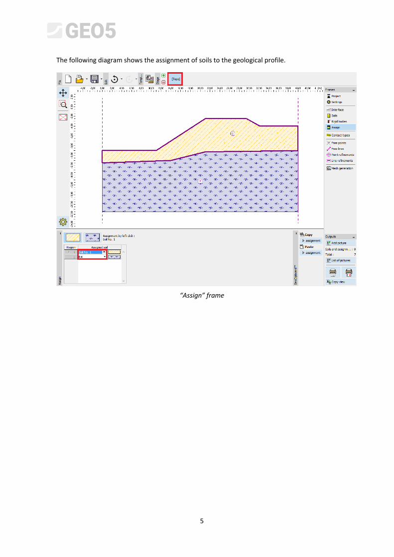
The following diagram shows the assignment of soils to the geological profile.

“Assign” frame

6

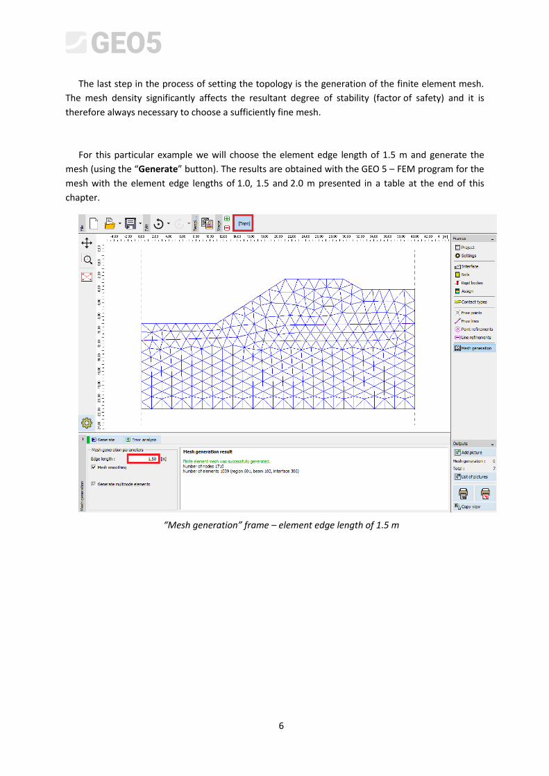
The last step in the process of setting the topology is the generation of the finite element mesh.

The mesh density significantly affects the resultant degree of stability (factor of safety) and it is

therefore always necessary to choose a sufficiently fine mesh.

For this particular example we will choose the element edge length of 1.5 m and generate the

mesh (using the “Generate” button). The results are obtained with the GEO 5 – FEM program for the

mesh with the element edge lengths of 1.0, 1.5 and 2.0 m presented in a table at the end of this

chapter.

“Mesh generation” frame – element edge length of 1.5 m

7

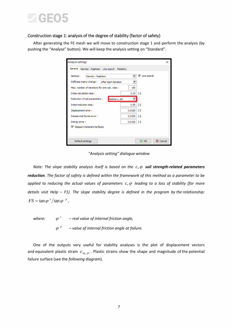
Construction stage 1: analysis of the degree of stability (factor of safety)

After generating the FE mesh we will move to construction stage 1 and perform the analysis (by

pushing the “Analyse” button). We will keep the analysis setting on “Standard”.

“Analysis setting” dialogue window

Note: The slope stability analysis itself is based on the ,c soil strength-related parameters

reduction. The factor of safety is defined within the framework of this method as a parameter to be

applied to reducing the actual values of parameters ,c leading to a loss of stability (for more

details visit Help – F1). The slope stability degree is defined in the program by the relationship:

psFS tantan ,

where: s – real value of internal friction angle,

p – value of internal friction angle at failure.

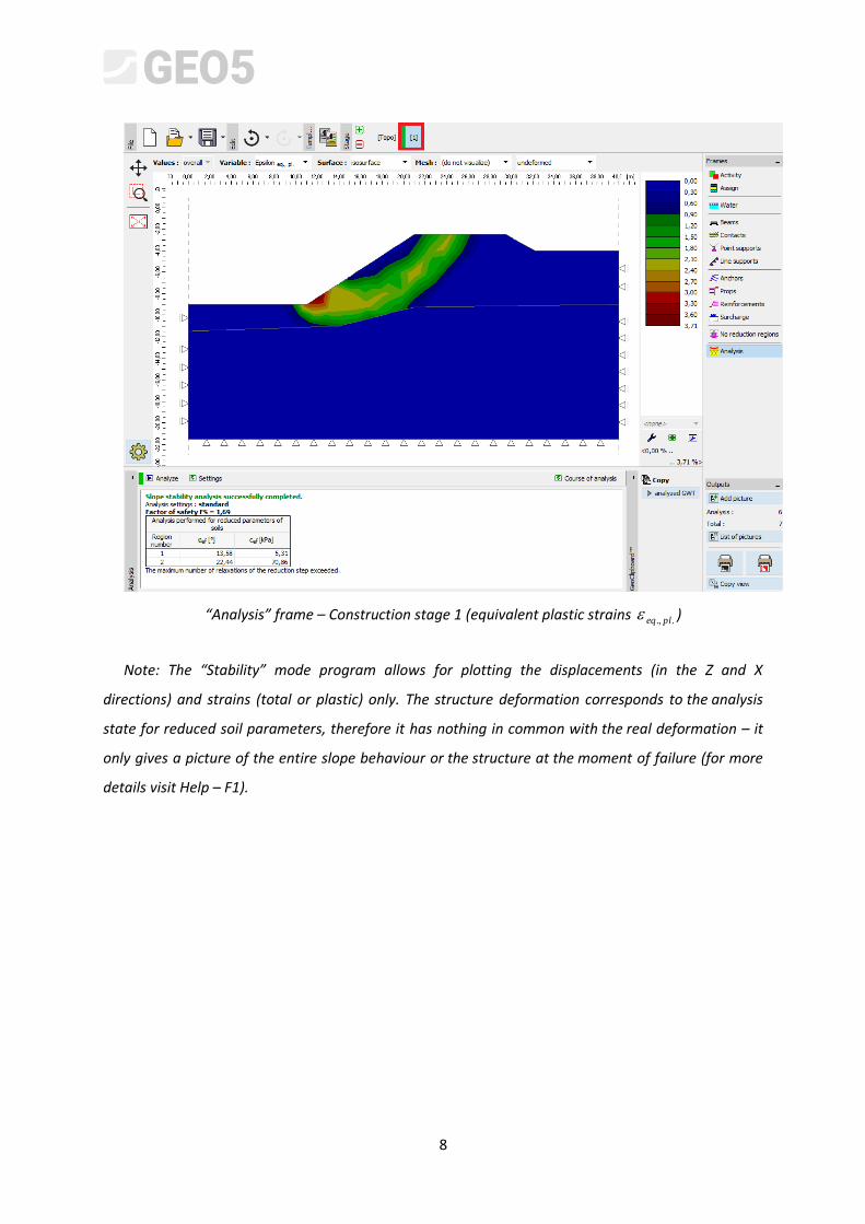
One of the outputs very useful for stability analyses is the plot of displacement vectors

and equivalent plastic strain .., pleq . Plastic strains show the shape and magnitude of the potential

failure surface (see the following diagram).

8

“Analysis” frame – Construction stage 1 (equivalent plastic strains .., pleq )

Note: The “Stability” mode program allows for plotting the displacements (in the Z and X

directions) and strains (total or plastic) only. The structure deformation corresponds to the analysis

state for reduced soil parameters, therefore it has nothing in common with the real deformation – it

only gives a picture of the entire slope behaviour or the structure at the moment of failure (for more

details visit Help – F1).

9

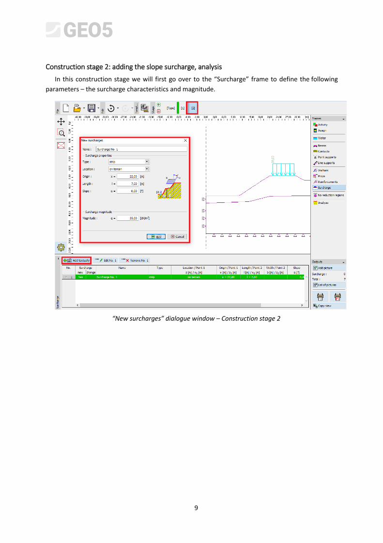
Construction stage 2: adding the slope surcharge, analysis

In this construction stage we will first go over to the “Surcharge” frame to define the following

parameters – the surcharge characteristics and magnitude.

“New surcharges” dialogue window – Construction stage 2

10

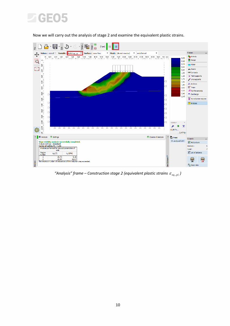
Now we will carry out the analysis of stage 2 and examine the equivalent plastic strains.

“Analysis” frame – Construction stage 2 (equivalent plastic strains .., pleq )

11

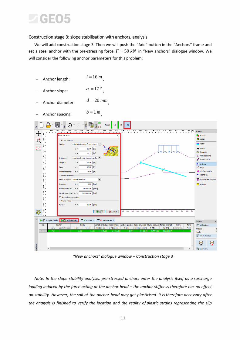
Construction stage 3: slope stabilisation with anchors, analysis

We will add construction stage 3. Then we will push the “Add” button in the “Anchors” frame and

set a steel anchor with the pre-stressing force kNF 50 in “New anchors” dialogue window. We

will consider the following anchor parameters for this problem:

Anchor length: ml 16 ,

Anchor slope: 17 ,

Anchor diameter: mmd 20 ,

Anchor spacing: mb 1 .

“New anchors” dialogue window – Construction stage 3

Note: In the slope stability analysis, pre-stressed anchors enter the analysis itself as a surcharge

loading induced by the force acting at the anchor head – the anchor stiffness therefore has no effect

on stability. However, the soil at the anchor head may get plasticised. It is therefore necessary after

the analysis is finished to verify the location and the reality of plastic strains representing the slip

12

surface. In the case of the soil under the anchor head getting plasticised, it is necessary to edit the

model (for more details visit Help – F1).

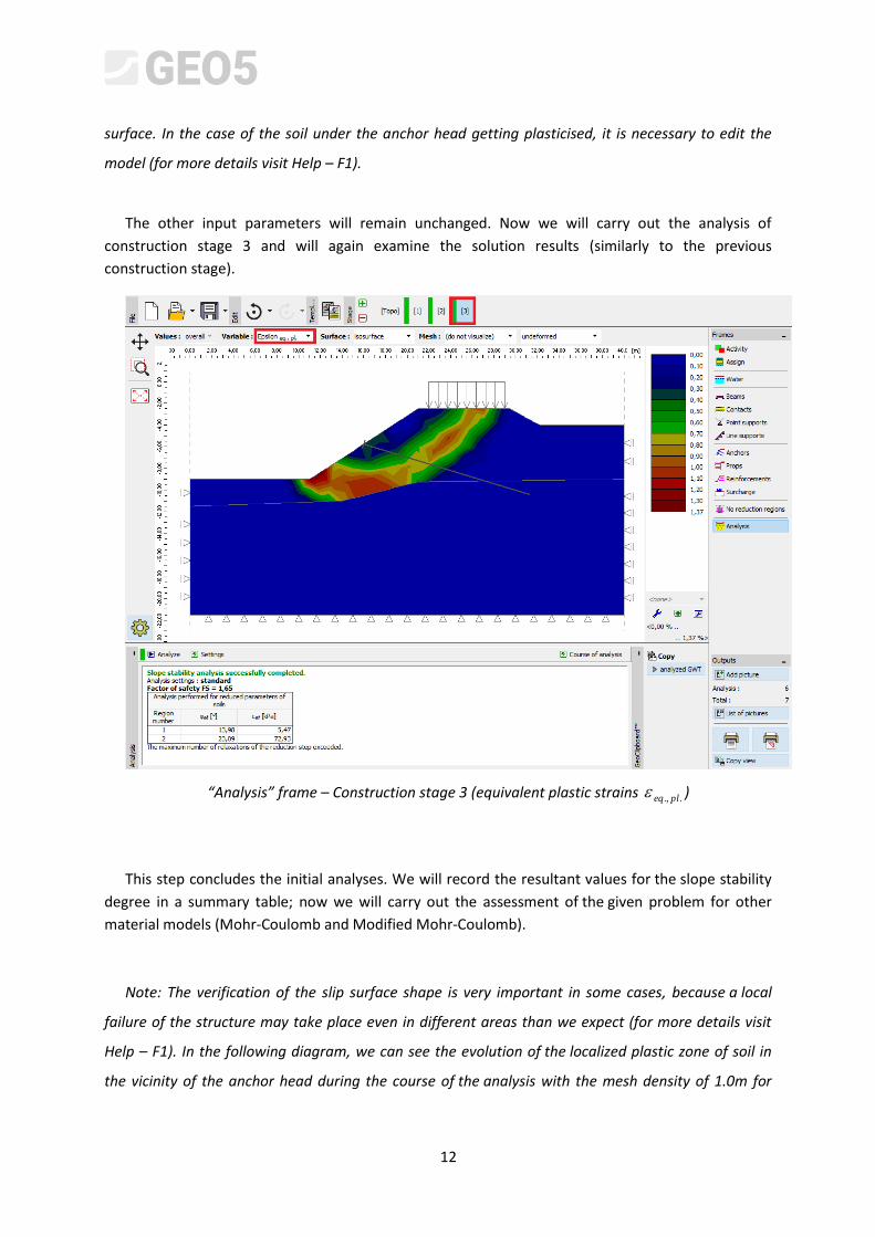
The other input parameters will remain unchanged. Now we will carry out the analysis of

construction stage 3 and will again examine the solution results (similarly to the previous

construction stage).

“Analysis” frame – Construction stage 3 (equivalent plastic strains .., pleq )

This step concludes the initial analyses. We will record the resultant values for the slope stability

degree in a summary table; now we will carry out the assessment of the given problem for other

material models (Mohr-Coulomb and Modified Mohr-Coulomb).

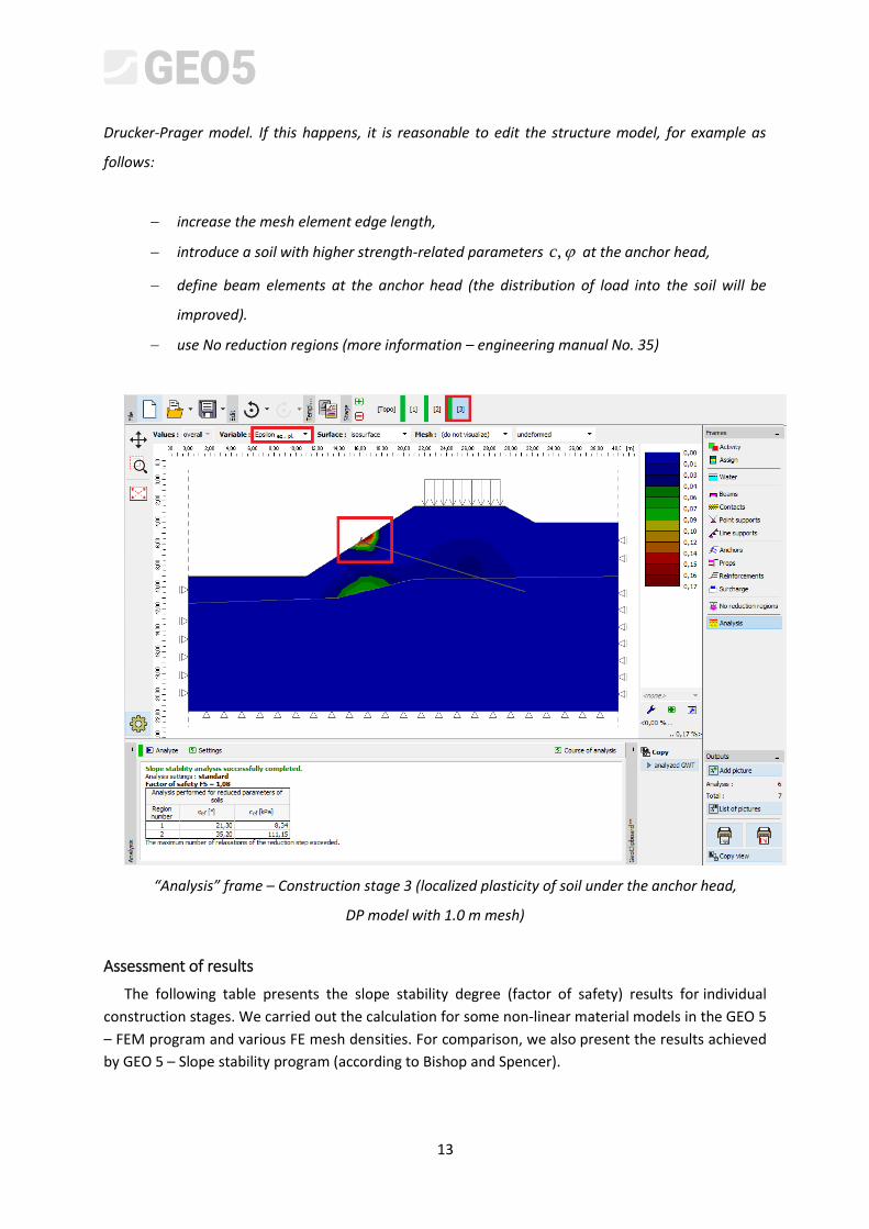
Note: The verification of the slip surface shape is very important in some cases, because a local

failure of the structure may take place even in different areas than we expect (for more details visit

Help – F1). In the following diagram, we can see the evolution of the localized plastic zone of soil in

the vicinity of the anchor head during the course of the analysis with the mesh density of 1.0m for

13

Drucker-Prager model. If this happens, it is reasonable to edit the structure model, for example as

follows:

increase the mesh element edge length,

introduce a soil with higher strength-related parameters ,c at the anchor head,

define beam elements at the anchor head (the distribution of load into the soil will be

improved).

use No reduction regions (more information – engineering manual No. 35)

“Analysis” frame – Construction stage 3 (localized plasticity of soil under the anchor head,

DP model with 1.0 m mesh)

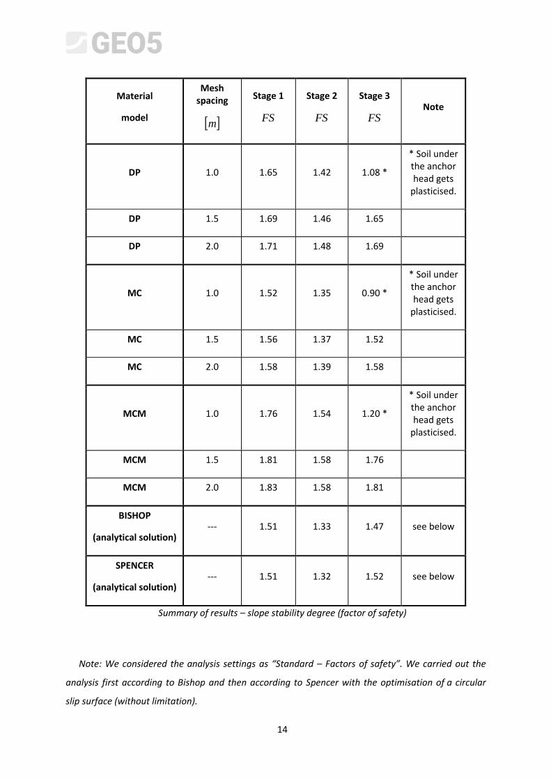
Assessment of results

The following table presents the slope stability degree (factor of safety) results for individual

construction stages. We carried out the calculation for some non-linear material models in the GEO 5

– FEM program and various FE mesh densities. For comparison, we also present the results achieved

by GEO 5 – Slope stability program (according to Bishop and Spencer).

14

Material

model

Mesh spacing

m

Stage 1

FS

Stage 2

FS

Stage 3

FS Note

DP 1.0 1.65 1.42 1.08 *

* Soil under the anchor head gets

plasticised.

DP 1.5 1.69 1.46 1.65

DP 2.0 1.71 1.48 1.69

MC 1.0 1.52 1.35 0.90 *

* Soil under the anchor head gets

plasticised.

MC 1.5 1.56 1.37 1.52

MC 2.0 1.58 1.39 1.58

MCM 1.0 1.76 1.54 1.20 *

* Soil under the anchor head gets

plasticised.

MCM 1.5 1.81 1.58 1.76

MCM 2.0 1.83 1.58 1.81

BISHOP

(analytical solution) --- 1.51 1.33 1.47 see below

SPENCER

(analytical solution) --- 1.51 1.32 1.52 see below

Summary of results – slope stability degree (factor of safety)

Note: We considered the analysis settings as “Standard – Factors of safety”. We carried out the

analysis first according to Bishop and then according to Spencer with the optimisation of a circular

slip surface (without limitation).

15

Conclusion

The following conclusion can be drawn from the numerical solution results:

The locally increased density of the FE mesh leads to more accurate results; on the other

hand, the duration of the analysis for each construction stage is extended.

It is necessary for the analyses to use non-linear material models,

allowing for the development of plastic strains.

Maximum equivalent plastic strains .., pleq express the locations where a potential slip

failure surface is located.