General rights Copyright and moral rights for the publications made accessible in the public portal are retained by the authors and/or other copyright owners and it is a condition of accessing publications that users recognise and abide by the legal requirements associated with these rights.

Users may download and print one copy of any publication from the public portal for the purpose of private study or research.

You may not further distribute the material or use it for any profit-making activity or commercial gain

You may freely distribute the URL identifying the publication in the public portal If you believe that this document breaches copyright please contact us providing details, and we will remove access to the work immediately and investigate your claim.

Downloaded from orbit.dtu.dk on: Feb 19, 2020

Oscillators - an approach for a better understanding

Lindberg, Erik

Published in:Proceedings ECCTD'03

Publication date:2003

Document VersionPublisher's PDF, also known as Version of record

Link back to DTU Orbit

Citation (APA):Lindberg, E. (2003). Oscillators - an approach for a better understanding. In Proceedings ECCTD'03

Oscillators - an approach for a better understanding

(tutorial presented at ECCTD’03)

Erik Lindberg, IEEE Lifemember ∗

Abstract — The aim of this tutorial is to provide anelectronic engineer knowledge and insight for a bet-ter understanding of the mechanisms behind the be-haviour of electronic oscillators. A linear oscillatoris a mathematical fiction which can only be used as astarting point for the design of a real oscillator basedon the Barkhausen criteria. Statements in textbooksand papers saying that the nonlinearities are bring-ing back the poles to the imaginary axis are wrong.The concept of ”frozen eigenvalues” is introduced bymeans of piece-wise-linear modelling of the nonlin-ear components which are necessary for steady stateoscillations. A number of oscillator designs are in-vestigated and the mechanisms behind the controlof frequency and amplitude are discussed.

1 Introduction and General Remarks

An oscillator is a physical system for which you mayobserve some kind of periodic behaviour. Nature isfilled with oscillators all the way from the super-strings of size 1e-33 to the galaxies in the universeof size 1e+33. Possibly the first human oscillatorexperiments were done many thousands years agowith mechanical oscillators (swings), acoustical os-cillators (tubes, flutes) or mixed mechacustic oscil-lators (drums, wind harps or small pieces of woodor bone rotating in the end of a string). Later whenthe wheel was invented water mills were examples ofhuman made oscillators. The first mechanical pre-cision oscillator was the pendulum clock inventedby C. Huygens (1629-1695) in 1656. Please see laterwhere an electronic analogue of the pendulum clockis discussed.

1.1 Amplifiers

Electronics was born in 1883 when T. A. Edisoninstalled a small metal plate near the filament inone of his incandescent lampbulbs. He applied acurrent to heat the filament and noticed that a gal-vanometer connected between the filament and theplate showed a current that flowed when the platewas at a positive potential with respect to the fila-ment. At that time nothing was known of electronsand the phenomena was referred to as the Edisoneffect. J. A. Fleming conducted experiments on the

∗Ørsted•DTU Department, 348 Technical Universityof Denmark, DK-2800 Kgs. Lyngby, Denmark, e-mail:el@oersted.dtu.dk, tel.: +45 4525 3650, fax: +45 45880117.

Edison effect from 1896 to 1901. He used the unidi-rectional flow of current between the cold plate andthe hot filament in his “Fleming Valve” or the vac-uum tube diode as it is known today. In 1906 Leede Forest introduced the grid between the filamentand the plate so that the flow of electrons couldbe controlled. This type of tube became known asthe triode. In its semiconductor version, the tran-sistor (J. Bardeen and W. H. Brattain 1948), it isthe basic element of electronic amplifiers. Also thetube diode has been replaced or supplemented withthe semiconductor diode dating back to the point-contact diodes of the “crystal” radio.

Today we are able to produce large integratedcircuits (SoC, Systems on Chips) which are able toperform almost any kind of signal processing. Theoperational amplifier is a simple integrated circuitwhich may be used as an almost ideal device forsignal amplification.

During the last 100 years electronic engineershave succeeded enormously by means of the as-sumption that the dc bias point of an amplifier istime invariant so that it may be used as referencefor the time varying signals, the linear small signalapproach or the linear blinkers approach. By meansof negative or degenerative feed back the amplifierperformance is improved by sacrifying gain.

1.2 Sinusoidal Oscillators

Concerning oscillators they are divided into twogroups according to the type of signal. Oscillatorsgenerating sinusoidal signals are termed ”linear” os-cillators. All other oscillators are termed relaxationor switching oscillators. ”Linear” oscillators arenormally considered second order systems. Manytopologies have been proposed for sinusoidal oscil-lators (Colpitts, Clapp, Hartley, Pierce etc.).

The design of a ”linear” oscillator is normallybased on the Barkhausen criteria [1] according towhich an oscillator is looked upon as an ideal finitegain amplifier with a linear frequency determiningfeed-back circuit (Fig. 1).

In order to startup the oscillations some param-eters of the circuit are adjusted so that the poles(eigenvalues) of the linearized circuit are in theright-half plane, RHP, i.e. in the dc bias point thecircuit is unstable and signals will start to increase

Figure 1: A negative resistance oscillator,“Barkhausen topology”.

when the power supply is connected. It is obvi-ous that if the poles initially are very close to theimaginary axis (high Q) the time constant is verylarge (days, months, years ?) and the transient timeto steady state behaviour is very large, i.e. appar-ently steady state sinusoidal oscillations take place.The placement of the poles on the imaginary axisis an impossible act of balance. The crucial pointis whether there will be oscillations or just a tran-sition to a new stable dc bias point. Very little isreported about how far out in the RHP the polesshould be placed initially.

In textbooks and papers you may find statementslike:

”A ”linear” oscillators is an amplifier with pos-itive or regenerative feed back for which theBarkhausen condition is satisfied at a particular fre-quency”

or”A ”linear” oscillator is an unstable amplifier for

which the nonlinearities are bringing back the ini-tial poles in the right half plane of the complexfrequency plane, RHP, to the imaginary axis”

or”There is always electrical noise in a circuit. The

frequency component of the noise corresponding tothe Barkhausen criteria will be amplified by thefeed back circuit so that the proper sine signalbuilds up. The nonlinearities will limit the extentto which the oscillations builds up”.

Apparently it is assumed that a ”linear” real os-cillator in the steady state behave like an ideal lin-ear mathematical harmonic lossless LC oscillatorwith a complex pole pair on the imaginary axis ofthe complex frequency plane. This is of course notthe case.

The aim of this tutorial is to investigate the be-

haviour of ”linear” oscillators by means of a studyof the movements of the poles of the ”linear” oscil-lator as function of time. This approach is calledthe frozen eigenvalues approach. The poles are theeigenvalues of the linearized Jacobian of the non-linear differential equations used as a mathemat-ical model for the ”linear” oscillator. By meansof piece-wise-linear modelling of the amplifier gain,i.e. large gain for small signals and gain zero forlarge signals, the ”linear” oscillator becomes linearin time slots so it make sense to calculate the poles.Please see later (Fig. 8) where a quadrature oscil-lator [8] is discussed.

2 Oscillators

An oscillator is a circuit which for constant inputsignal (dc battery) produce an oscillating outputsignal (a steady state time varying signal). An oldrule of thumb says that if you want to design anoscillator try to design an amplifier instead and ifyou want to design an amplifier try to design anoscillator (violation of Murphys Law).

The ideal mathematical linear harmonic oscilla-tor may be realized in principle as an electronic cir-cuit by means of a coil L and a capacitor C coupledin parallel (or in series). With the initial condi-tions: a charge on the capacitor and no current inthe coil, the voltage of the capacitor will be a cosineand the current of the coil a sine function of timewith constant amplitudes.

The eigenvalues of the Jacobian of the two cou-pled first order differential equations of the coil andthe capacitor are on the imaginary axis (no losses)and the oscillator may start up with any initial con-dition with no transition to the steady state. Thisis of course mathematical fiction. It is impossibleto realize in the real world an oscillator having thepoles on the imaginary axis for all times. It is animpossible act of balance to fix the poles on theimaginary axis. Real oscillators must rely on non-linearities.

Figure 2: A damped linear oscillator.

In the real world coils and capacitors are alwaysconnected with loss mechanisms which as a firstsimple model may be inserted as a resistor Rs inseries with the coil and a conductor Gp in parallelwith the capacitor as shown in Fig. 2.

If you introduce a negative conductance in par-allel with Gp you may compensate the losses andmake the coefficient to s zero or negative so thatthe poles are on the imaginary axis or in RHP.

The characteristic polynomial of the linear dif-ferential equations describing the circuit becomes

s2 + 2 α s + ω20 = 0 ,

where

2 α =(

Rs

L+

Gp

C

)

and

ω20 =

1 + RsGp

L C.

The poles or the natural frequencies of the circuit- the eigenvalues of the Jacobian of the differentialequations - are the roots of the characteristic poly-nomial.

p1,2 = − α ± j√

ω20 − α2 = − α ± j ω .

With certain initial conditions: flux in connec-tion with the coil and charge in connection withthe capacitor, damped voltages and currents maybe observed. The damping of the signals is givenby the factor e−αt . If ω2

0 > α2 the poles are com-plex and the signals become damped sine and cosinefunctions of the time A× e−α t × sin(ωt + ϕ).

Figure 3: An amplifier with positive and negativefeed-back.

In order to obtain undamped signals - steadystate signals - we must introduce an energy source(battery) and some kind of electronic component(transistor, operational amplifier) which may am-plify signals.

Figure 3 shows a general linear amplifier withpositive and negative feed-back. The inputimpedance of the amplifier is assumed infinite andthe gain of the amplifier is assumed constant, i.e.V3 = A (V1 − V2).

If we observe time varying signals for zero inputsignal Vin = 0 we have an oscillator. If the polesof the linearized circuit are in the left half plane(LHP) of the complex frequency plane the signalsare damped. If the poles are in RHP the signals areundamped. Only if the poles are on the imaginaryaxis the signals are steady state signals. This is ofcourse impossible in a real world circuit. The idealharmonic oscillator may be started with any ini-tial condition and keep its amplitude and frequencyconstant with no initial transient.

If we want to build an oscillator we must intro-duce an amplifier with nonlinear gain so that forsmall signals the poles of the linearized circuit arein RHP and for large signals the poles are in LHP.In this case we may obtain steady state behaviourbased on balance between energy we obtain fromthe battery when the poles are in RHP and energywe loose when the poles are in LHP.

In other words an oscillator is a feed-back ampli-fier with an unstable dc bias point. Due to the non-linear components the linearized small signal modelcorresponding to the instant bias point will varywith time. The dominating behaviour of the cir-cuit is based on the instant placement of the polesof the linearized model. If the poles are in RHP thesignals will increase in amplitude. If the poles arein LHP the signals will diminish in amplitude.

Seen from the source Vin the load is

Z = ZD + ZC

(ZB + ZA (1−A)ZA + ZB (1 + A)

).

If we introduce memory elements - capacitors,coils, hysteresis - in the four impedances varioustypes of oscillators may be obtained [2].

If we replace the impedances ZA, ZB and ZC

with resistors RA, RB and RC and introduce anoperational amplifier with large gain A for smallinput signals and zero gain for large input signalsthe admittance Y in parallel with ZD becomes

Y =(

1RC

)(RA + RB (1 + A)RB + RA (1−A)

),

which for A = 0 gives

Y =1

RC,

and for A very large (positive or negative) gives

Y = − RB

RARC.

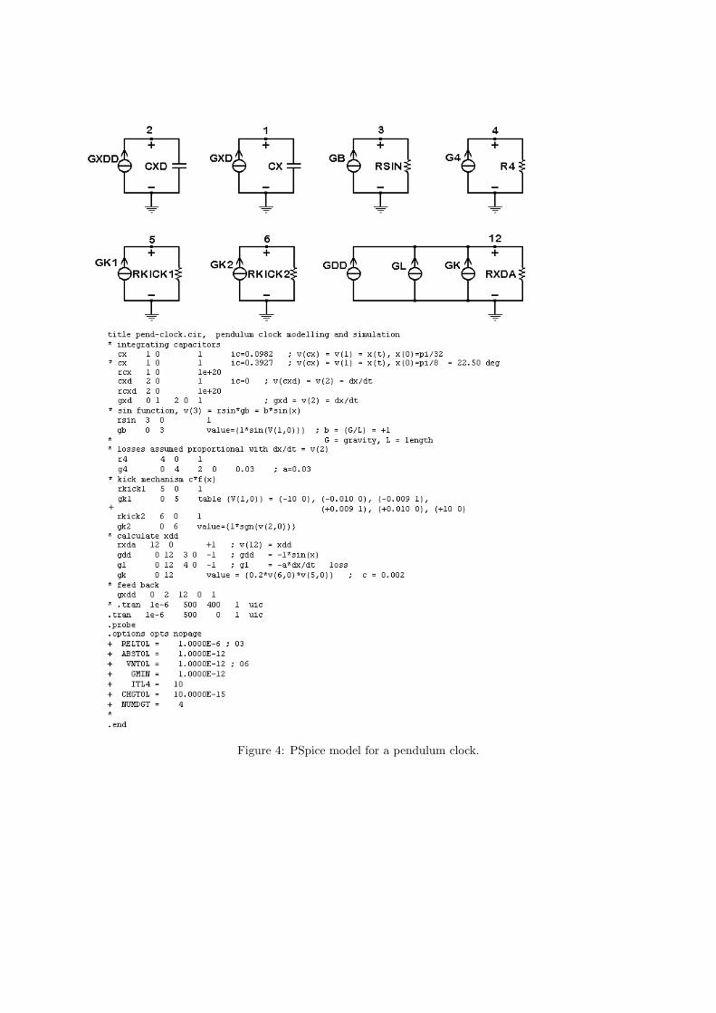
Figure 4: PSpice model for a pendulum clock.

It is seen that for small signals we have anegative conductance in parallel with ZD and forlarge signals we have a positive conductance.

Here the feed-back is simplified to voltage divi-sion. In the general voltage feed-back case a threeterminal two-port may be used and the impedancesused here become two of the three impedances inthe Π-equivalent of the two-port. Similar investi-gations may be used for the three other kinds offeed-back and for other kinds of amplifiers.

3 EXAMPLES

The Pendulum ClockTwo Quadrature Oscillators

Vidal’s Quadrature OscillatorMancini’s Quadrature OscillatorA Negative Resistance Oscillator

A Wien Bridge OscillatorA Common Multi-vibrator

3.1 The Pendulum Clock

The pendulum clock with unit mass may be mod-eled with the following second order differentialequation

d2x

dt2+ a ∗ dx

dt+ b ∗ sin(x) = c ∗ f(x)

where x is the angle from vertical. The losses aremodeled by the constant a. The constant b = G/Lis the ratio between gravity G and length L. Forsmall values of x the pendulum is ”kicked” by thefunction c∗f(x) by means of the escapement mech-anism when the weights go down a step changingpotential energy into a kinetic energy impulse. Themodel may easily be changed into two coupled firstorder differential equations with x and dx

dt as theprimary variables.

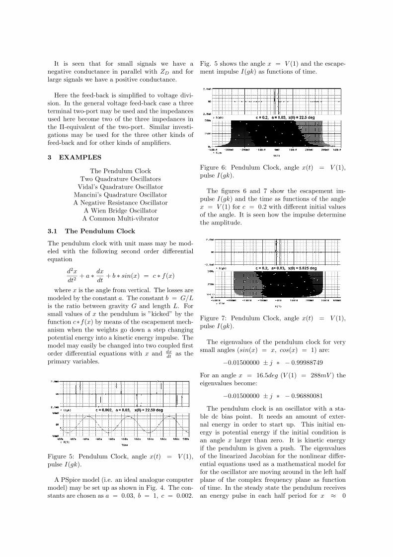
Figure 5: Pendulum Clock, angle x(t) = V (1),pulse I(gk).

A PSpice model (i.e. an ideal analogue computermodel) may be set up as shown in Fig. 4. The con-stants are chosen as a = 0.03, b = 1, c = 0.002.

Fig. 5 shows the angle x = V (1) and the escape-ment impulse I(gk) as functions of time.

Figure 6: Pendulum Clock, angle x(t) = V (1),pulse I(gk).

The figures 6 and 7 show the escapement im-pulse I(gk) and the time as functions of the anglex = V (1) for c = 0.2 with different initial valuesof the angle. It is seen how the impulse determinethe amplitude.

Figure 7: Pendulum Clock, angle x(t) = V (1),pulse I(gk).

The eigenvalues of the pendulum clock for verysmall angles (sin(x) = x, cos(x) = 1) are:

−0.01500000 ± j ∗ − 0.99988749

For an angle x = 16.5deg (V (1) = 288mV ) theeigenvalues become:

−0.01500000 ± j ∗ − 0.96880081

The pendulum clock is an oscillator with a sta-ble dc bias point. It needs an amount of exter-nal energy in order to start up. This initial en-ergy is potential energy if the initial condition isan angle x larger than zero. It is kinetic energyif the pendulum is given a push. The eigenvaluesof the linearized Jacobian for the nonlinear differ-ential equations used as a mathematical model forfor the oscillator are moving around in the left halfplane of the complex frequency plane as functionof time. In the steady state the pendulum receivesan energy pulse in each half period for x ≈ 0

when the the weights go down controlled by theescapement. The size of this pulse determine themaximum swing. For small swing the movement isvery close to sinusoidal.

3.2 Two Quadrature Oscillators

Quadrature oscillators are based on a feed-backloop with at least one almost ideal integrator forwhich input and output are two sinusoids with 90degree phase difference. In [7] an active RC inte-grator and a passive RC integrator are combinedwith a negative resistance. The mechanism with acomplex pole pair moving between RHP and LHPmay be observed.

3.2.1 Vidal’s Quadrature Oscillator

If two amplifiers are coupled as shown in Fig. 8 youmay have a quadrature oscillator if the impedancesare chosen as resistors according to [8]. In this caseyou make use of the operational amplifier poles asfrequency determining memory (“integrating realpoles”) and the nonlinear saturation characteristicof the operational amplifier as the amplitude limit-ing mechanism.

Figure 8: Quadrature Oscillator.

The quadrature oscillator is made from three cir-cuits. For the first circuit (Z1, Z2 and A1) youhave:

V3

V1=

1 + R2R1

1 + 1A1

(1 + R2

R1

)

.For the second circuit (Z3, Z4, Z5, Z6 and A2) youhave:

V6

V3=

1(1 + R3

R4

) (R5

R5+R6− 1

A2

)− R3

R4

.The third circuit is the feed-back circuit (Z7 andZ8) for which:

V1

V6=

R7

R7 + R8

. The loop gain is the product of the three networkfunctions.

With reference to [8] you may now design theoscillator. With R1 = R4 = R7 = 10kΩ you getR2 = 33.5kΩ, R3 = R8 = 3kΩ, R5 = 1Ω andR6 = 1130Ω. Figure 9 shows the result of a PSpiceanalysis with two µA741 Op Amps. The frequencyis 530kHz and the output amplitude of any of thetwo Op Amps is 155mV.

Figure 9: Quadrature Oscillator. V(3) as functionof V(6).

Figure 10: Op Amp macro model. Eout = A(s)Vac,ω1 = 197.77, ω2 = 68.375M.

Figure 11: Comparison of the open loop ac-transfercharacteristics of the Op Amp macro model of Fig.10 and the PSpice µA741 library macro model.Amplitude characteristic. Logarithmic frequencyscale.

Figure 10 shows a simple macro model for theOp Amp with two negative real poles. The fig-ures 11 and 12 show the result of an optimiza-tion of the simple model with only one nonlinearelement: the piece wise linear voltage controlled

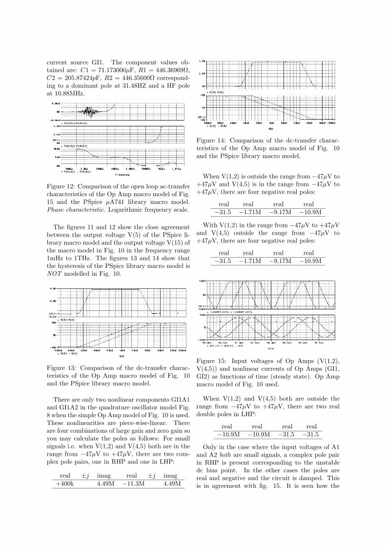
current source GI1. The component values ob-tained are: C1 = 71.173000µF, R1 = 446.36969Ω,C2 = 205.87424pF, R2 = 446.35600Ω correspond-ing to a dominant pole at 31.48HZ and a HF poleat 10.88MHz.

Figure 12: Comparison of the open loop ac-transfercharacteristics of the Op Amp macro model of Fig.15 and the PSpice µA741 library macro model.Phase characteristic. Logarithmic frequency scale.

The figures 11 and 12 show the close agreementbetween the output voltage V(5) of the PSpice li-brary macro model and the output voltage V(15) ofthe macro model in Fig. 10 in the frequency range1mHz to 1THz. The figures 13 and 14 show thatthe hysteresis of the PSpice library macro model isNOT modelled in Fig. 10.

Figure 13: Comparison of the dc-transfer charac-teristics of the Op Amp macro model of Fig. 10and the PSpice library macro model.

There are only two nonlinear components GI1A1and GI1A2 in the quadrature oscillator model Fig.8 when the simple Op Amp model of Fig. 10 is used.These nonlinearities are piece-wise-linear. Thereare four combinations of large gain and zero gain soyou may calculate the poles as follows: For smallsignals i.e. when V(1,2) and V(4,5) both are in therange from −47µV to +47µV, there are two com-plex pole pairs, one in RHP and one in LHP:

real ±j imag real ±j imag+400k 4.49M −11.3M 4.49M

Figure 14: Comparison of the dc-transfer charac-teristics of the Op Amp macro model of Fig. 10and the PSpice library macro model.

When V(1,2) is outside the range from −47µV to+47µV and V(4,5) is in the range from −47µV to+47µV, there are four negative real poles:

real real real real−31.5 −1.71M −9.17M −10.9M

With V(1,2) in the range from −47µV to +47µVand V(4,5) outside the range from −47µV to+47µV, there are four negative real poles:

real real real real−31.5 −1.71M −9.17M −10.9M

Figure 15: Input voltages of Op Amps (V(1,2),V(4,5)) and nonlinear currents of Op Amps (GI1,GI2) as functions of time (steady state). Op Ampmacro model of Fig. 10 used.

When V(1,2) and V(4,5) both are outside therange from −47µV to +47µV, there are two realdouble poles in LHP:

real real real real−10.9M −10.9M −31.5 −31.5

Only in the case where the input voltages of A1and A2 both are small signals, a complex pole pairin RHP is present corresponding to the unstabledc bias point. In the other cases the poles arereal and negative and the circuit is damped. Thisis in agreement with fig. 15. It is seen how the

two op amps synchronize so that only one OpAmp is active at a time. A certain amount ofenergy is moving between the memory elementscorresponding to the input level of 47µV abovewhich the gain is zero.

Vidal’s quadrature oscillator is an oscillator withan unstable dc bias point (complex pole pair inRHP). In the steady state the poles apparentlyare real and negative all the time. The system isdamped but for small signals energy is deliveredfrom the power supply as pulses the same way thependulum clock receives the energy from gravity.

Figure 16: Quadrature Oscillator (16).

3.2.2 Mancini’s Quadrature Oscillator

Figure 16 shows a quadrature oscillator made fromtwo active and one passive integrator [3].

The characteristic polynomial for the linearizeddifferential equations becomes:

s3 +

s2

(G2

C2+

G1

C1

1(1 + A1)

+G3

C3

1(1 + A2)

)+

s

(G1G2

C1C2

A1A2

(1 + A1) (1 + A2)

)+

s

(G1G2

C1C2

1(1 + A1)

+G2G3

C2C3

1(1 + A2)

)+

s

(G1G3

C1C3

1(1 + A1) (1 + A2)

)+

G1G2G3

C1C2C3

(1 + A1A2)(1 + A1) (1 + A2)

Figure 17: Linear Op Amp quadrature oscillator(A = 100k). Output V(3) and V(6) as function ofOp Amp A2 input V(4,5).

For A1 = A2 = 100k, R1 = R2 = R3 = R =10kΩ and C1 = C2 = C3 = C = 10nF the charac-teristic polynomial becomes:

s3 + s2

(1

RC

)(1.00002000) +

s

(1

RC

)2

(1.00000000) +(

1RC

)3

(0.9999800004)

where 1RC = 10k so oscillation occurs at ω = 2πf =

10k, f = 1.59kHz, T = 0.628ms.

Figure 18: Nonlinear Op Amp quadrature oscillator(A = µA741). Output V(3) and V(6) as functionof Op Amp A2 input V(4,5).

The figures 17 and 18 show the outputs V(3) andV(6) as function of the Op Amp A2 input V(4,5) forthe linear and the nonlinear model of the quadra-ture oscillator. It is seen that the linear model isslightly unstable.

The upper part of Fig. 19 shows that stableoscillations take place. The lower part of Fig. 19shows that heavy pulses occur at the op am inputs.

Mancini’s quadrature oscillator is an oscillatorfor which a complex pole pair apparently are closeto the imaginary axis all the time. It is reported byMancini [3] that the outputs V(3) and V(6) haverelatively high distortion which means that a gain

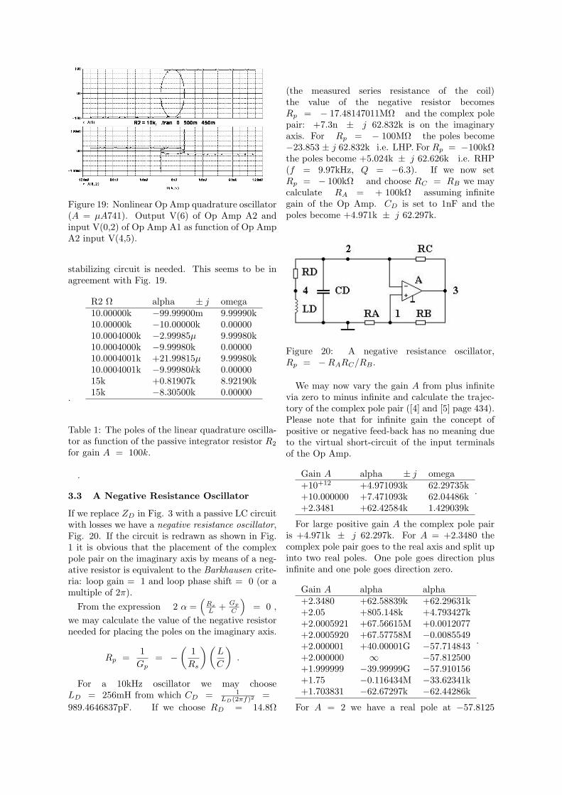
Figure 19: Nonlinear Op Amp quadrature oscillator(A = µA741). Output V(6) of Op Amp A2 andinput V(0,2) of Op Amp A1 as function of Op AmpA2 input V(4,5).

stabilizing circuit is needed. This seems to be inagreement with Fig. 19.

R2 Ω alpha ± j omega10.00000k −99.99900m 9.99990k10.00000k −10.00000k 0.0000010.0004000k −2.99985µ 9.99980k10.0004000k −9.99980k 0.0000010.0004001k +21.99815µ 9.99980k10.0004001k −9.99980kk 0.0000015k +0.81907k 8.92190k15k −8.30500k 0.00000.

Table 1: The poles of the linear quadrature oscilla-tor as function of the passive integrator resistor R2

for gain A = 100k.

.

3.3 A Negative Resistance Oscillator

If we replace ZD in Fig. 3 with a passive LC circuitwith losses we have a negative resistance oscillator,Fig. 20. If the circuit is redrawn as shown in Fig.1 it is obvious that the placement of the complexpole pair on the imaginary axis by means of a neg-ative resistor is equivalent to the Barkhausen crite-ria: loop gain = 1 and loop phase shift = 0 (or amultiple of 2π).

From the expression 2 α =(

Rs

L + Gp

C

)= 0 ,

we may calculate the value of the negative resistorneeded for placing the poles on the imaginary axis.

Rp =1

Gp= −

(1

Rs

)(L

C

).

For a 10kHz oscillator we may chooseLD = 256mH from which CD = 1

LD(2πf)2 =989.4646837pF. If we choose RD = 14.8Ω

(the measured series resistance of the coil)the value of the negative resistor becomesRp = − 17.48147011MΩ and the complex polepair: +7.3n ± j 62.832k is on the imaginaryaxis. For Rp = − 100MΩ the poles become−23.853 ± j 62.832k i.e. LHP. For Rp = −100kΩthe poles become +5.024k ± j 62.626k i.e. RHP(f = 9.97kHz, Q = −6.3). If we now setRp = − 100kΩ and choose RC = RB we maycalculate RA = + 100kΩ assuming infinitegain of the Op Amp. CD is set to 1nF and thepoles become +4.971k ± j 62.297k.

Figure 20: A negative resistance oscillator,Rp = −RARC/RB .

We may now vary the gain A from plus infinitevia zero to minus infinite and calculate the trajec-tory of the complex pole pair ([4] and [5] page 434).Please note that for infinite gain the concept ofpositive or negative feed-back has no meaning dueto the virtual short-circuit of the input terminalsof the Op Amp.

Gain A alpha ± j omega+10+12 +4.971093k 62.29735k+10.000000 +7.471093k 62.04486k+2.3481 +62.42584k 1.429039k

.

For large positive gain A the complex pole pairis +4.971k ± j 62.297k. For A = +2.3480 thecomplex pole pair goes to the real axis and split upinto two real poles. One pole goes direction plusinfinite and one pole goes direction zero.

Gain A alpha alpha+2.3480 +62.58839k +62.29631k+2.05 +805.148k +4.793427k+2.0005921 +67.56615M +0.0012077+2.0005920 +67.57758M −0.0085549+2.000001 +40.00001G −57.714843+2.000000 ∞ −57.812500+1.999999 −39.99999G −57.910156+1.75 −0.116434M −33.62341k+1.703831 −62.67297k −62.44286k

.

For A = 2 we have a real pole at −57.8125

and the other real pole is infinite. Please notethat “infinite” and “zero” in a sense is the same“number”. The two poles now go together forA = 1.703831 and leaves the real axis as a complexpole pair with decreasing real part and increasingimaginary part.

Gain A alpha ± j omega+1.703830 −62.55769k 0.123544k+1.5 −35.02890k 51.80031k+1.0000000 −15.02890k 60.68044k+0.5 −8.362239k 61.94583k+1µ −5.028911k 62.30199k+10−24 −5.028906k 62.30199k+0 −1.695572k 62.47853k

.

For A = 0 the complex pole pair is

−1.695572k ± j 62.47853k.

It is seen that for positive gain (A > 0) the mech-anism behind the negative resistance oscillator isrelaxation for the component values chosen.

For negative values of the gain the complexpole pair moves further from LHP to RHP. ForA = − 2.0232555 the complex pole pair passesthe imaginary axis. For negative gain (A < 0) thepoles moves smoothly across the imaginary axis asit e.g. is seen for the Colpitts oscillator [6].

Gain A alpha ± j omega−10−24 −5.028906k 62.30199k−1µ −5.028901k 62.30199k−0.5000000 −3.028906k 62.42934k−1.0000000 −1.695572k 62.47853k−2.0000000 −28.906250 62.49999k−2.0230000 −0.3206173 62.49997k−2.0232550 −5.521610m 62.49997k−2.0232600 +0.656338m 62.49997k−2.10 +93.044969 62.49981k−2.5 +526.64930 62.49726k−10.0 +3.304427k 62.40949k−1k +4.951133k 62.29896k−10+12 +4.971093k 62.29735k

.

The behaviour for positive and negative valuesof the gain A has been verified by means of PSpicesimulation with RC4136 Op Amp by monitoringthe current in the negative resistance.

By means of experiments with PSpice for varia-tion of the resistors RB and RC the distortion ofthe amplifier may be minimized.

3.4 A Wien Bridge Oscillator

If we in Fig. 3 replace ZA with RA in parallel withCA, ZB with RB in series with CB , ZC with RC

and ZD with RD we have a Wien Bridge Oscillator.

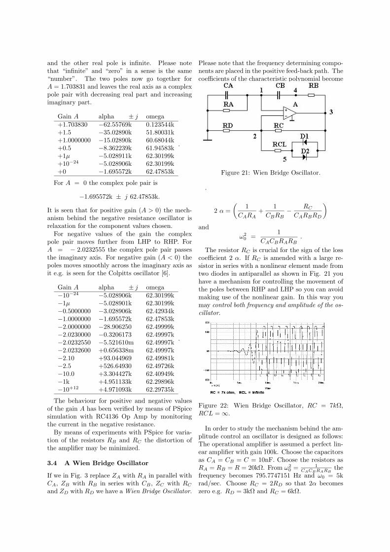
Please note that the frequency determining compo-nents are placed in the positive feed-back path. Thecoefficients of the characteristic polynomial become

Figure 21: Wien Bridge Oscillator.

.

2 α =(

1CARA

+1

CBRB− RC

CARBRD

)

andω2

0 =1

CACBRARB.

The resistor RC is crucial for the sign of the losscoefficient 2 α. If RC is amended with a large re-sistor in series with a nonlinear element made fromtwo diodes in antiparallel as shown in Fig. 21 youhave a mechanism for controlling the movement ofthe poles between RHP and LHP so you can avoidmaking use of the nonlinear gain. In this way youmay control both frequency and amplitude of the os-cillator.

Figure 22: Wien Bridge Oscillator, RC = 7kΩ,RCL = ∞.

In order to study the mechanism behind the am-plitude control an oscillator is designed as follows:The operational amplifier is assumed a perfect lin-ear amplifier with gain 100k. Choose the capacitorsas CA = CB = C = 10nF. Choose the resistors asRA = RB = R = 20kΩ. From ω2

0 = 1CACBRARB

thefrequency becomes 795.7747151 Hz and ω0 = 5krad/sec. Choose RC = 2RD so that 2α becomeszero e.g. RD = 3kΩ and RC = 6kΩ.

RC Ω alpha ± j omega12k +4.99937k 79.052410k +3.33286k 3.72719k9k +2.49960k 4.33035k8k +1.66633k 4.71416k→ 7k +833.055 4.93011k6100.00 +83.1033 4.99930k6010.00 +8.10783 4.99999k6003.00 +2.27485 4.99999k6002.00 +1.44157 4.99999k6001.00 +0.60829 4.99999k6000.270008101 +6.31994e− 10 5.00000k6000.270008100 −1.99284e− 10 5.00000k5999.00 −1.05827 4.99999k5998.00 −1.89155 4.99999k5990.00 −8.55782 4.99999k5900.00 −83.5533 4.99930k→ 5k −833.511 4.93003k4k −1.66680k 4.71399k3k −2.50009k 4.33006k2k −3.33340k 3.72671k1k −4.16671k 2.76378k800.00 −4.33337k 2.49436k600.00 −4.50003k 2.17937k400.00 −4.66669k 1.79497k200.00 −4.83336k 1.28008k100.00 −4.91669k 908.91450.00 −4.95835k 643.95225.00 −4.97919k 455.68210.00 −4.99169k 288.1195.00 −4.99585k 203.4661.00 −4.99919k 89.9028.

Table 2: The poles of the linear Wien bridge oscil-lator as function of resistor RC .

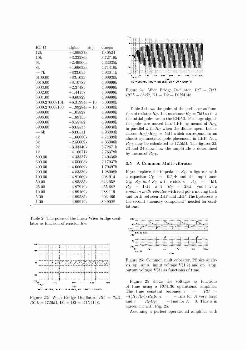
Figure 23: Wien Bridge Oscillator, RC = 7kΩ,RCL = 17.5kΩ, D1 = D2 = D1N4148.

Figure 24: Wien Bridge Oscillator, RC = 7kΩ,RCL = 38kΩ, D1 = D2 = D1N4148.

Table 2 shows the poles of the oscillator as func-tion of resistor RC . Let us choose RC = 7kΩ so thatthe initial poles are in the RHP 2. For large signalsthe poles are moved into LHP by means of RCL

in parallel with RC when the diodes open. Let uschoose RC//RCL = 5kΩ which correspond to analmost symmetrical pole placement in LHP. NowRCL may be calculated as 17.5kΩ. The figures 22,23 and 24 show how the amplitude is determinedby means of RCL.

3.5 A Common Multi-vibrator

If you replace the impedance ZD in figure 3 witha capacitor CD = 0.5µF and the impedancesZA, ZB and ZC with resistors RA = 1kΩ,RB = 1kΩ and RC = 2kΩ you have acommon multi-vibrator with real poles moving backand forth between RHP and LHP. The hysteresis isthe second “memory component” needed for oscil-lations.

Figure 25: Common multi-vibrator, PSpice analy-sis, op. amp. input voltage V(1,2) and op. amp.output voltage V(3) as functions of time.

Figure 25 shows the voltages as functionsof time using a RC4136 operational amplifier.The time constant becomes τ = RC =−((RARC)/RB)CD = − 1ms for A very largeand τ = RCCD = + 1ms for A = 0. This is inagreement with Fig. 25.

Assuming a perfect operational amplifier with

Figure 26: Multi-vibrator pole as function of am-plifier gain A.

gain A the pole of the circuit is +1k for A verylarge and −1k for A very little. For A = 2 thepole pass from +∞ to −∞ as shown in Fig. 26.Please note that this is not a jump but a smoothtransition.

4 CONCLUSIONS

”Linear” oscillators are nonlinear electronic cir-cuits.

The nonlinearities do not bring back the poles tothe imaginary axis.

The oscillator amplitude may be controlled byother means than the power supply.

If you place the poles as close as possible to theimaginary axis you may obtain a noisy oscillator

At a certain instant the linearized small signalmodel of an oscillator will try to oscillate accordingto the poles. The actual oscillator frequency is akind of an average frequency.

In this tutorial it is demonstrated that it ispossible to obtain insight in the mechanisms be-hind the behaviour of oscillators by means ofthe frozen eigenvalues approach. We must rewriteour textbooks and replace ”obscure noise state-ments” and statements concerning ”nonlinearitiespulling the poles back to the imaginary axis” withproper statements concerning the mechanisms be-hind the steady state oscillations as e.g. sinusoidaloscillation where a complex pole pair is movingbetween RHP and LHP or relaxation oscillationwhere real poles are moving between RHP andLHP.

Apparently there are three basic types of oscilla-tors. The first type has an unstable initial dc biaspoint. This type is selfstarting when the power sup-ply is connected. The poles are moving betweenRHP and LHP so that a balance is obtained be-

tween the energy obtained from the power supplywhen the poles are in RHP and the energy lost whenthe poles are in LHP.

The second type has a stable initial dc bias point.This type needs some extra initial energy in orderto start up. The poles are in LHP all the timeand some special impulse mechanism is needed toprovide energy from the power supply in the steadystate.

The third type is a combination of the two types.It is unstable in the initial dc bias point and thepoles are moving around in LHP only in the steadystate.

Electromechanical crystal oscillators should beinvestigated with the presented technique in the fu-ture.

References

[1] H. Barkhausen, Lehrbuch der Elektronen-Rohre, 3.Band, “Ruckkopplung” , Verlag S.Hirzel, 1935.

[2] J. R. Westra, C. J. M. Verhoeven and A. H. M.van Roermund, Oscillators and Oscillator Sys-tems - Classification, Analysis and Synthesis,pp. 1-282, Kluwer 1999.

[3] Ron Mancini (edt. in Chief), Op Amps ForEveryone, Design Reference, slod006b, TexasInstruments, August 2002,http://focus.ti.com/docs/apps/catalog/resources/appnoteabstract.jhtml?abstractName=slod006b.

[4] E. Lindberg, “Oscillators and eigenvalues”, inProceedings ECCTD’97 - The 1997 EuropeanConference on Circuit Theory and Design, pp.171-176, Budapest, September 1997.

[5] L. Strauss, Wave Generation and Shaping, pp.1-520, McGraw-Hill, 1960.

[6] E. Lindberg, “Colpitts, eigenvalues andchaos”, in Proceedings NDES’97 - the 5’th In-ternational Specialist Workshop on NonlinearDynamics of Electronic Systems, pp. 262-267,Moscow, June 1997.

[7] A.S. Sedra and K.C. Smith, MicroelectronicCircuits 4th Ed, Oxford University Press,1998.

[8] E. Vidal, A. Poveda and M. Ismail, “Describ-ing Functions and Oscillators”, IEEE Circuitsand Devices, Vol. 17, No. 6, pp. 7-11, Novem-ber 2001.