Orders, Production, and Inventory Investment · Volume Title: Orders, Production, and Investment: A...
66
This PDF is a selection from an out-of-print volume from the National Bureau of Economic Research Volume Title: Orders, Production, and Investment: A Cyclical and Structural Analysis Volume Author/Editor: Victor Zarnowitz Volume Publisher: NBER Volume ISBN: 0-870-14215-1 Volume URL: http://www.nber.org/books/zarn73-1 Publication Date: 1973 Chapter Title: Orders, Production, and Inventory Investment Chapter Author: Victor Zarnowitz Chapter URL: http://www.nber.org/chapters/c3555 Chapter pages in book: (p. 344 - 408)
Transcript of Orders, Production, and Inventory Investment · Volume Title: Orders, Production, and Investment: A...

This PDF is a selection from an out-of-print volume from the National Bureauof Economic Research
Volume Title: Orders, Production, and Investment: A Cyclical and StructuralAnalysis
Volume Author/Editor: Victor Zarnowitz
Volume Publisher: NBER
Volume ISBN: 0-870-14215-1
Volume URL: http://www.nber.org/books/zarn73-1
Publication Date: 1973
Chapter Title: Orders, Production, and Inventory Investment
Chapter Author: Victor Zarnowitz
Chapter URL: http://www.nber.org/chapters/c3555
Chapter pages in book: (p. 344 - 408)
8ORDERS, PRODUCTION, AND
INVENTORY INVESTMENT
THERE ARE THREE major sections in this chapter. The first is a theoret-ical discussion of the major determinants of purchasing and inventorybehavior. The second, a critical survey of recent work in inventoryanalysis, concentrates on the role of orders and related factors and onthe importance of disaggregation by type of production and stage offabrication. The third assembles and evaluates additional evidence onthe relations that underlie the cyclical fluctuations of inventories.
Determinants and Patterns of Inventory Behavior
Relations with Sales and Orders Placed and OutstandingWe will consider orders relating to goods that are to be resold by the
buyer in unchanged physical form, e.g., orders for a consumer goodreceived by the producer from the distributor.' Let us suppose thatwe have data for the purchasing firm on (1) the sales of the product ineach consecutive planning period ("month"); (2) the orders for theproduct placed by the firm each month with its suppliers; (3) the vol-ume of such orders outstanding at the end of each month; and (4) thestock of the product in possession of the firm at the end of each month.To abstract from problems of measurement and aggregation, assumethat all these series are in homogeneous physical units of the given
'Some of what follows can, with modifications, be applied to the buying of goods to be resoldafter processing, e.g., to materials purchasing by the manufacturer. The restriction adopted abovewill help to keep the analysis simple. Investment in purchased materials will be taken up in thefollowing section.
Orders, Production, and Inventory Investment 345
good. A number of different models based on such data can be de-vised, embodying certain more or less simple assumptions about therelations among the four variables. The few such models presentedhere, while no doubt highly oversimplified, are nevertheless instructive(see Chart 8-1 and Table 8-1).
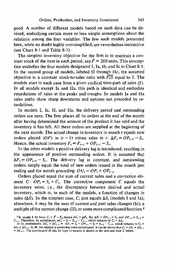
The simplest inventory objective for the firm is to maintain a con-stant stock of the item in each period, say F — 200 units. This assump-tion underlies the four models designated I, Ia, Ib, and Ic in Chart 8-1.In the second group of models, labeled II through lic, the assumedobjective is a constant stock-to-sales ratio with equal to 2. Themodels start in each case from a given cyclical time-path of sales (S).In all models except Ia and ha, this path is identical and embodiesretardations of sales at the peaks and troughs. In models Ia and hasales paths show sharp downturns and upturns not preceded by re-tardations.
In models I, Ia, II, and ha, the delivery period and outstandingorders are zero. The firm places all its orders at the end of the monthafter having determined the amount of the product it has sold and theinventory it has left. All these orders are supplied at the beginning ofthe next month. The actual change in inventory in month t equals neworders placed (OP) in (t — 1) minus sales in t: = —
Hence, the actual inventory = + —
In the other models a positive delivery lag is introduced, resulting inthe appearance of positive outstanding orders. It is assumed thqt
= — The delivery lag is constant, and outstandingorders simply equal the total of new orders issued in the month justending and the month preceding: = OP1 +
Orders placed equal the sum of current sales and a correction ele-ment C: OP1 = + C equals theinventory error, i.e., the discrepancy between desired and actualinventory, which is, in each of the models, a function of changes insales In the simplest case, just equals (models I and Ia);elsewhere, it may be the sum of current and past sales changes (Ic), amultiple of the current change (II), or some more complicated function.2
2 In model I we have = P — F1; hence = But AF1 = — and 0P1_, = S,_1 +Therefore, by substitution, = S1 — S,_1 — which reduces to
In Ic, analogously, + = —AF€ = — 0P1_2 = — S1_2 — C1_2, which reduces to =+ In lb. the relation is somewhat more complicated. It can be shown that C = ±
+ The counterpart of this for type 11 models is shown in the text and note 3, beLow.

346 Causes and Implications of Changes in Unfilled Orders and Inventories
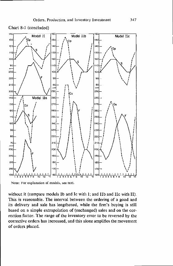
It follows that orders placed depend on the level of sales and onchanges in sales. The latter corrective component imparts to the be-havior of orders (in relation to sales) the well-known characteristicsof acceleration and magnification. For cyclically fluctuating series suchas sales, levels and changes are positively correlated. Hence orders,being directly related to both the level of and the first differences insales, exceed sales in amplitude of fluctuation (compare the curves Sand OP in the upper panels of Chart 8-1). But there are differences.The magnification of the movement of orders in comparison with prod-uct sales is greater in the models with a delivery lag than in those
Chart 8-1Cyclical Time-Paths of Sales, Orders Placed and Outstanding,
and Product Inventory in Eight Hypothetical Models
S = salesOp = new orders placedOu = outstanding purchase ordersF = product inventory
140 14C
Model 1 Model Lb Model Ic130— 130— / 130—
/ / 'pp
200 270 — 270
130 - /\OpModel La : I' ::i A
:: :1'/:3::!'
F /
I II II I I II III Ill I II 1111 II 1111 II I II II12345678 10 12 14 12345678 10 12 14 12345678 10 12 14
Orders, Production, and Inventory Investment 347
Chart 8-1 (concluded)
Note: For explanation of models, see text.
without it (compare models lb and Ic with I; and lIb and lIc with II).This is reasonable. The interval between the ordering of a good andits delivery and sale has lengthened, while the firm's buying is stillbased on a simple extrapolation of (unchanged) sales and on the cor-rection factor. The range of the inventory error to be reversed by thecorrective orders has increased, and this alone amplifies the movementof orders placed.
Model Uc
- --
Mode) 11130 — ,/ \ I
100 \\ /90 —
220 —A210 —
200
Mode) libA
150—
I
I
tI
I I
I
II II I
II I
I
I
I I
I I
I
I II
I I
I
I
150
I
S.
80 —
290 —
280 —
270 — t\OuF
/ t260— 1
250—
240—
II
1F
I
I I1
I I
230
220
210_/
200
I II
— S
II
/I
— I I
I II'
II
I
190—
180—
I
II I
II I
170—IlItlIlIllIll
140 — Model l[a
530— \Qp/I i
120 — I
110
100
90 I
— 'III80—
70 —
220 —
210 —
200
12345678 10 12 14 12345678 10 12 14 12345678 50 12 14

Tab
le 8
-1D
ata
Inpu
t and
Out
put f
or E
ight
Mod
els
of S
ales
-Ord
ers-
Inve
ntor
y R
elat
ions
Period b
Var
iabl
eand Modela
12
34
56
78
910
11
12
13
14
SAL
ES
(S)C
1,Ib
,lc;I
I,llb
,IIc
lOOT
105
110
115
120
120
120?
115
110
105
100
lOOT
105
110
Ia
lOOT
105
112
125P
115
110
lOOT
105
112
ha
100
105
112
120?
115
110
lOOT
105
112
NEW
OR
DE
RS
PLA
CE
D (
OP)
1100
110
115
120
125P
120
120
110
105
100
95T
100
100
115
lb
100
110
125
135
135P
120
105
95
95T
100
100
100
110
125
ic
100
110
120
125
130P
125
120
110
100
95
90T
95
110
120
ii
100
120
125
130
135?
120
120
100
95
90
85T
100
120
125
hib
100
120
145
155P
145
110
85
75T
85
100
100
100
120
145
lIc
100
120
130
135
140P
125
120
100
90
85
SOT
95
120
130
Ia
100
110
119
138?
111
102
90T
110
119
ha
100
120
133
144P
100
95
70T
120
133
INVENTORY
(F)d
I200
195
195
195
195T
200
200
205
205
205
205P
200
195
195
lb
200
195
185
180T
185
200
215
220P
215
205
200
200
195
185
Ic
200
195
185
180
180T
185
195
205
215
220
220P
215
200
185
II
200
195T
205
215
225
240
240
245P
235
225
215
200
195T
205
hIb
200
195
185T
190
215
250
275P
270
245
215
200
200
195
185T
lie
200
195
185T
190
200
215
235
245
255?
250
240
225
200
185T
Ia
200
195
193
187T
207
208
210P
195
193
ha
200
195T
203
216
245P
235
230
195T
203
OUTSTANDING
OR
DE
RS
(OU
)dlb
200
210
235
260
270P
255
225
200
190T
195
200
200
210
235
Ic
200
210
230
245
255
255?
245
230
210
195
185
185T
205
230
hIb
200
220
265
300
300?
255
195
160
160T
185
200
200
220
265
lIe
200
220
250
265
275P
265
245
220
190
175
165T
175
215
250
Orders, Production, and Inventory Investment 349
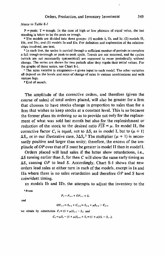
Notes to Table 8-1
P peak; T trough. In the case of high or low plateaus of equal value, the laststanding is taken to be the peak or trough.
a The models are divided into three groups: (1) models I, Ib, and Ic; (2) models II,lib, and lic; and (3) models Ia and ha. For definition and explanation of the relation-ships involved, see text.
b In each line, the series is carried through a sufficient number of periods to completea full trough-to-trough or peak-to-peak cycle. Trends are not assumed, and the cycles(which are not necessarily symmetrical) are supposed to recur periodically withoutchange. The series are shown for two periods after they regain their initial values. Forthe graphs of these series, see Chart 8-1.
c The sales variable is exogenous—a given input to each model. The other variablesall depend on the levels and rates of change of sales in various combinations and withvarious lags.
d End of month.
The amplitude of the corrective orders, and therefore (given thecourse of sales) of total orders placed, will also be greater for a firmthat chooses to have stocks change in proportion to sales than for afirm that wishes to keep stocks at a constant level. This is so becausethe former plans its ordering so as to provide not only for the replace-ment of what was sold last month but also for the replenishment orreduction of the stock to the desired ratio = In model II, thecorrective factor C1 is equal, not to as in model I, but to + 1)
or in our illustrative case, The multiplier + 1) is neces-sarily positive and larger than unity; therefore, the excess of the am-plitude of OP over that of S must be greater in model II than in model I.
Orders placed will lead sales if the latter show retardations, i.e.,turning earlier than S, for then C will show the same early timing ascausing OP to lead S. Accordingly, Chart 8-I shows that new
orders lead sales at either turn in each of the models, except in Ia andha where there is no sales retardation and therefore OP and S havecoin'.ident timing.
in models Lb and JIb, the attempts to adjust the inventory to the
3From
F1 = + + S.
and
= + C,_1 = S1_1 + —
we obtain by substitution F1 = (I + — S1; and
C1 + S=(I +
350 Causes and Implications of Changes in Unfilled Orders and Inventories
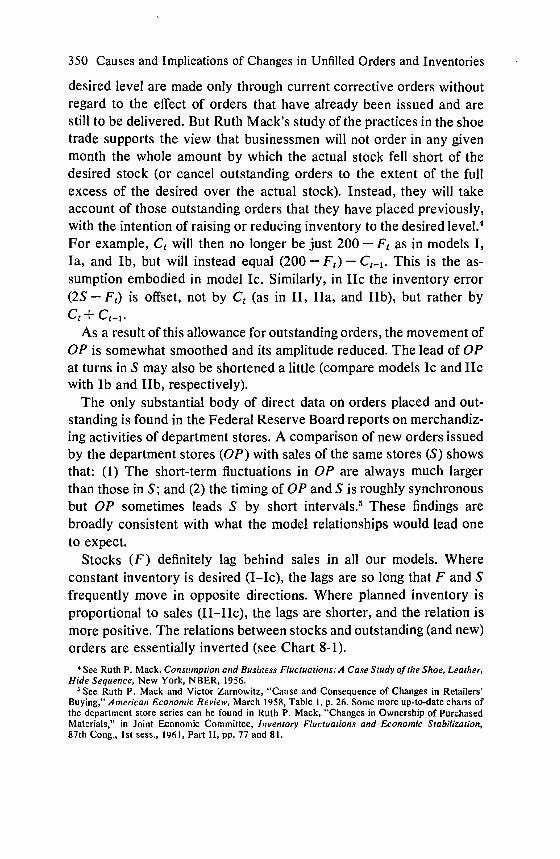
desired level are made only through current corrective orders withoutregard to the effect of orders that have already been issued and arestill to be delivered. But Ruth Mack's study of the practices in the shoetrade supports the view that businessmen will not order in any givenmonth the whole amount by which the actual stock fell short of thedesired stock (or cancel outstanding orders to the extent of the fullexcess of the desired over the actual stock). Instead, they will takeaccount of those outstanding orders that they have placed previously,with the intention of raising or reducing inventory to the desired level.4For example, will then no longer be just 200 — as in models I,Ia, and Ib, but will instead equal (200 — — This is the as-sumption embodied in model Ic. Similarly, in lic the inventory error(2S — is offset, not by (as in II, ha, and JIb), but rather byct+
As a result of this allowance for outstanding orders, the movement ofOP is somewhat smoothed and its amplitude reduced. The lead of OPat turns in S may also be shortened a little (compare models Ic and licwith lb and JIb, respectively).
The only substantial body of direct data on orders placed and out-standing is found in the Federal Reserve Board reports on merchandiz-ing activities of department stores. A comparison of new orders issuedby the department stores (OP) with sales of the same stores (S) showsthat: (1) The short-term fluctuations in OP are always much largerthan those in S; and (2) the timing of OP and S is roughly synchronousbut OP sometimes leads S by short intervals.5 These findings arebroadly consistent with what the model relationships would lead oneto expect.
Stocks (F) definitely lag behind sales in all our models. Whereconstant inventory is desired (I—Ic), the lags are so long that F and Sfrequently move in opposite directions. Where planned inventory isproportional to sales (Il—lic), the lags are shorter, and the relation ismore positive. The relations between stocks and outstanding (and new)orders are essentially inverted (see Chart 8-1).
Ruth P. Mack, Consumption and Business Fluctuations: A Case Study of the Shoe, Leather,Hide Sequence, New York, NBER, 1956.
See Ruth P. Mack and Victor Zarnowitz, "Cause and Consequence of Changes in Retailers'Buying," American Economic Review, March 1958, Table 1, p. 26. Some more up-to-date charts ofthe department store series can be found in Ruth P. Mack, "Changes in Ownership of PurchasedMaterials," in Joint Economic Committee, Inventory Fluctuations and Economic Stabilization,87th Cong., 1st sess., 1961, Part II, pp. 77 and 81.

Orders, Production, and Inventory Investment 351
Stocks undoubtedly lag behind sales in the department store data:They lagged at each of the six turns in sales in 194 1—54. But the lagswere not long (they averaged 2.3 months), and the relation was basi-cally positive rather than inverted.6 Relative to orders placed and out-standing, stocks show longer lags and correspondingly somewhatstronger inverted characteristics. Here the evidence is less favorableto our models but on the whole still not inconsistent with them.
Factors Influencing Purchases and Stocks of MaterialsConsider now the purchase of goods for use in production rather
than resale. Inventory of purchased materials (M) increases whenorders for materials placed by the firm (OM) are filled, that is, aretranslated into deliveries to the firm (DM). Inventory M decreaseswhen materials are withdrawn as input for production (IN). Therefore,
(1)
If the materials are supplied with delivery lag k, then 0 Mt_k =so
+ OMt_k — INS. (la)
Outstanding orders for materials (OUM) increase (decrease) whenorders placed exceed (fall short of) receipts, that is,
= + — (2)
Substituting the order terms from (2) for in (1), one gets
= + — + — INS. (3)
Following Ruth Mack, the sum of inventory and outstanding ordersfor materials will be called the "ownership" of purchased materials.Let this aggregate of stocks on hand and on order be denoted as
= + Then (3) can be rewritten as
OWMg = + — INS. (3a)
Definitional equations such as these of course tell us nothing directlyabout human behavior or testable economic relationships, but they canhelp to identify the roles of the variables concerned and to avoid someomissions and inconsistencies. Thus (3) and (3a) suggest that it is not
6 Mack and Zarnowitz, "Cause and Consequence."
0

352 Causes and Implications of Changes in Unfilled Orders and Inventories
only the levels and changes of stocks on hand that matter in the analy-sis of investment in purchased-materials inventories, but also the levelsand changes of stocks on order (outstanding purchase orders).7
The models of the preceding section suggest that sales-related goalsand variables have a central role in shaping the changes in inventories.While sales have been treated as exogenous, this is clearly not neces-sary; for example, sales expectations based on past sales behaviorcould well be explicitly introduced.8 In the equations for materials, itis the productive inputs (IN) that have a role analogous to that of sales(S) in the earlier models. The materials stock (M) here corresponds tothe "product inventory" (F) there, and the orders variables, OM andOUM, correspond to OP and OU, respectively. By substituting M forF, etc., the models could, mutatis mutandis, be adapted to reflect therelations among materials stocks, inputs, and orders. The magnifica-tion and acceleration effects would then be observed in the comparisonof movements in IN and OM; also, stocks on order would again befound to move ahead of stocks on hand.
The rates of utilization for materials (IN) depend primarily on theplanned production and its requirements. In manufacture to order, thescheduling of production is geared to orders received, their terms ofdelivery, and the progress of work on them: in other words, to the rel-evant dimensions of the firm's unfilled commitments to its customers.Manufacturers' shipments are closely correlated with output, and theycan be fairly well estimated as weighted totals of past, and perhaps alsocurrent, inflows of new orders (Chapter 5). Hence, these order re-ceipts, along with the distribution of the product delivery lags i,provide the main guide to the estimates of future output and of theassociated materials inputs (IN).
In production to stock, sales anticipations sa are presumably themain factor in short-term production planning. While "autonomous"expectations based on some "inside knowledge," guesswork, hopes,and the like, are probably often involved in the formation of Se', themajor observable determinant here is past sales experience. That is,
point received early and strong recognition in the writings of Ruth P. Mack (see notes 4 and5, above).
In a "complete" macro model, sales would be taken to depend on total output or income, and afeedback effect of inventory investment on sales and income would be included. Such models havebeen developed in the basic and influential articles by Lloyd A. Metzler, "The Nature and Stabilityof Inventory Cycles," Review of Economic Statistics, August 1941, and "Factors Governing theLength of Inventory Cycles," ibid., February 1947; and Ragnar Nurkse, "The Cyclical Pattern ofInventory Investment," Quarterly Journal of Economics. August 1952.
0
Orders, Production, and Inventory Investment 353
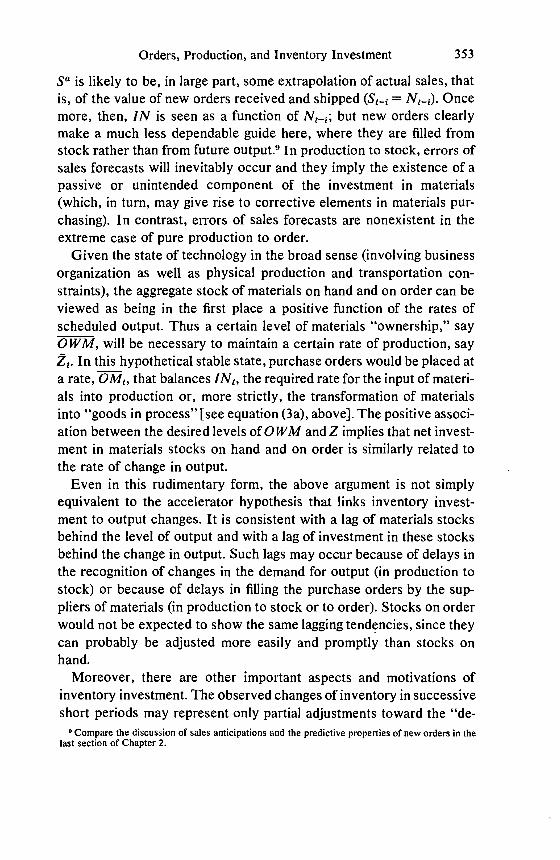
sa is likely to be, in large part, some extrapolation of actual sales, thatis, of the value of new orders received and shipped = Oncemore, then, IN is seen as a function of but new orders clearlymake a much less dependable guide here, where they are filled fromstock rather than from future output.9 In production to stock, errors ofsales forecasts will inevitably occur and they imply the existence of apassive or unintended component of the investment in materials(which, in turn, may give rise to corrective elements in materials pur-chasing). In contrast, errors of sales forecasts are nonexistent in theextreme case of pure production to order.
Given the state of technology in the broad sense (involving businessorganization as well as physical production and transportation con-straints), the aggregate stock of materials on hand and on order can beviewed as being in the first place a positive function of the rates ofscheduled output. Thus a certain level of materials "ownership," sayOWM, will be necessary to maintain a certain rate of production, say
In this_hypothetical stable state, purchase orders would be placed ata rate, that balances INS, the required rate for the input of materi-als into production or, more strictly, the transformation of materialsinto "goods in process" Ejsee equation (3a), above]. The positive associ-ation between the desired levels of OWM andZ implies that net invest-ment in materials stocks on hand and on order is similarly related tothe rate of change in output.
Even in this rudimentary form, the above argument is not simplyequivalent to the accelerator hypothesis that links inventory invest-ment to output changes. It is consistent with a lag of materials stocksbehind the level of output and with a lag of investment in these stocksbehind the change in output. Such lags may occur because of delays inthe recognition of changes in the demand for output (in production tostock) or because of delays in filling the purchase orders by the sup-pliers of materials (in production to stock or to order). Stocks on orderwould not be expected to show the same lagging tendencies, since theycan probably be adjusted more easily and promptly than stocks onhand.
Moreover, there are other important aspects and motivations ofinventory investment. The observed changes of inventory in successiveshort periods may represent only partial adjustments toward the "de-
° Compare the discussion of sales anticipations and the predictive properties of new orders in thelast section of Chapter 2.
354 Causes and Implications of Changes in Unfilled Orders and Inventories
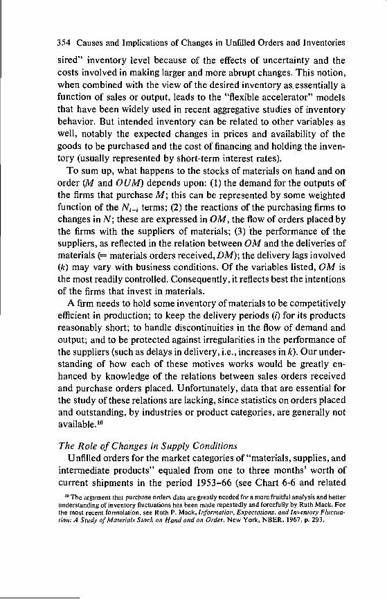
sired" inventory level because of the effects of uncertainty and thecosts involved in making larger and more abrupt changes. This notion,when combined with the view of the desired inventory as. essentially afunction of sales or output, leads to the "flexible accelerator" modelsthat have been widely used in recent aggregative studies of inventorybehavior. But intended inventory can be related to other variables aswell, notably the expected changes in prices and availability of thegoods to be purchased and the cost of financing and holding the inven-tory (usually represented by short-term interest rates).
To sum up, what happens to the stocks of materials on hand and onorder (M and OUM) depends upon: (1) the demand for the outputs ofthe firms that purchase M; this can be represented by some weightedfunction of the terms; (2) the reactions of the purchasing firms tochanges in N; these are expressed in OM, the flow of orders placed bythe firms with the suppliers of materials; (3) the performance of thesuppliers, as reflected in the relation between OM and the deliveries ofmaterials (= materials orders received, DM); the delivery lags involved(k) may vary with business conditions. Of the variables listed, OM isthe most readily controlled. Consequently, it reflects best the intentionsof the firms that invest in materials.
A firm needs to hold some inventory of materials to be competitivelyefficient in production; to keep the delivery periods (i) for its productsreasonably short; to handle discontinuities in the flow of demand andoutput; and to be protected against irregularities in the performance ofthe suppliers (such as delays in delivery, i.e., increases in k). Our under-standing of how each of these motives works would be greatly en-hanced by knowledge of the relations between sales orders receivedand purchase orders placed. Unfortunately, data that are essential forthe study of these relations are lacking, since statistics on orders placedand outstanding, by industries or product categories, are generally notavailable. 10
The Role of Changes in Supply ConditionsUnfilled orders for the market categories of "materials, supplies, and
intermediate products" equaled from one to three months' worth ofcurrent shipments in the period 195 3—66 (see Chart 6-6 and related
10 The argument that purchase orders data are greatly needed for a more fruitful analysis and betterunderstanding of inventory fluctuations has been made repeatedly and forcefully by Ruth Mack. Forthe most recent formulation, see Ruth P. Mack, information, Expectations, and Inventory Fluctua-(ion: A Study of Materials Stock on Hand and on Order, New York, NBER, 1967, p. 293.
Orders, Production, and Inventory Investment 355
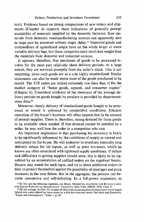
text). Evidence based on timing comparisons of new orders and ship-ments (Chapter 4) supports these indications of generally promptavailability of materials supplied by the domestic factories. Raw ma-terials from domestic nonmanufacturing sources can apparently alsoin large part be procured without major delay.'1 Imported goods andcommodities of agricultural origin have on the whole larger or morevariable delivery lags, but these categories carry much less weight thanthe materials from domestic and industrial sources.
It appears, therefore, that purchases of goods to be processed in-volve for the most part relatively short delivery periods; to a largeextent, they are serviced promptly from the seller's stock. This is notsurprising, since such goods are as a rule highly standardized. Similarstatements can also be made about most of the goods purchased to beresold. The U/S ratios are indeed extremely low (less than 1) for themarket category of "home goods, apparel, and consumer staples"(Chapter 6). Consistent evidence of the shortness of the average de-livery periods on goods bought by retailers is provided by department-store data.12
Moreover, timely delivery of standardized goods bought to be proc-essed or resold is enforced by competitive conditions. Efficientoperation of the buyer's business will often require that he be assuredof prompt supplies. There is, therefore, strong demand for these goodsto be available when needed. If that demand cannot be satisfied by aseller, he may well lose the order to a competitor who can.
An important implication is that purchasing for inventory is likelyto be significantly influenced by the conditions of supply as viewed andanticipated by the buyer. He will endeavor to avoid any unusually longdelivery delays for his inputs, as well as price increases, which heknows are often associated with tightened supply conditions. If delaysand difficulties in getting supplies should arise, this is likely to be sig-nalized by an accumulation of unfilled orders on the suppliers' books.Buyers may watch for such signs, and try to place additional orders intime to protect themselves against the possibility of shortages and priceincreases in the near future. But in the aggregate, the process can be-come cumulative and self-defeating. In a full-grown expansion, as
"On this and the following statement, see Moses Abramovitz, Inventories and Business Cycleswith Special Reference to Manufacturers' Inventories, New York, NBER, 1950, Chap. 9.
12 On the average, in 1941—54, receipts of (deliveries of merchandise to) department stores laggedbehind new orders placed by these stores by a little less than one month. See Mack and Zarnowitz,"Cause and Consequence," Table I, p. 26.

356 Causes and Implications of Changes in Unfilled Orders and Inventories
suppliers approach capacity operations they begin to quote longer"lead times" to their customers. To the extent that the latter respondby placing more orders in an attempt to increase their stocks on order,their actions, designed to alleviate the problem for the individual firm,are apt to aggravate the total problem. As the additional orders onlysucceed in swelling the suppliers' backlogs, they actually result in anintensified excess demand situation of which the increases in backlogs,delivery lags, and prices are primary symptoms.
However, some stabilizing forces are also at work in this process.Buyers basically prefer shorter delivery periods, and the competitionamong producer-sellers works toward satisfying this preference. Priceincreases may deter some buying. Moreover, just as the buyers watchthe backlogs of the suppliers, so may the latter watch the materialsstocks of the buyers. When these stocks run low, suppliers are likely toexpect an expansion of customer orders and might prepare for it invarious ways. Production to stock, in anticipation of the rise in orders,would be one such way, and would have a stabilizing effect.'3
During contractions, conversely, sales decrease and with them thedesired levels of stocks on hand and on order. Firms accordingly re-duce their current purchases, thereby gradually liquidating their out-standing orders, which are also the unfilled commitments of theirsuppliers. The delivery periods are thus cut back to their normal levels,which for much of inventory buying means immediate availability orvery short lead times. As the downward adjustment of stocks is com-pleted, there is no more reason for further reduction of purchases,unless sales continue declining. But in the early stages of contraction,the cessation of advance buying will have motivated some inventorydisinvestment and contributed to the business decline.
The interaction of changes in buyers' anticipations and ordering andof changes in supply conditions has long been neglected by the inven-tory theory. The theme has, however, received considerable attentionin some recent studies.'4
It should be noted, however, that large customer stocks are a phenomenon associated withproduction to order. (The major example is steel products, which are largely manufactured to orderand the inventories of which are heavily concentrated in user hands.) In industries that are predomi-nantly engaged in manufacture to order, low levels of customer-held stocks may not be a sufficientinducement for the producers to switch, on a large scale, to production to stock.
"In addition to the previously cited books by Mack and the article by Mack and Zarnowitz, seeThomas M. Stanback,Jr., Postwar Cycles in Manufacturers' Inventories, New York, NBER, 1962.

Orders, Production, and Inventory Investment 357
The Effects of Backlog ChangesThe preceding discussion of the effect of changes in supply condi-
tions and anticipations on buying of materials and stocks in trade wouldlead one to predict a positive association between backlog changes andinventory investment. Such a relation has indeed been repeatedly ob-served, but in a form which admits (or even demands) a different inter-pretation.
Manufacturers who accumulate unfilled orders can look forward toincreased sales and, to the extent that the backlogs represent firmcommitments, will indeed feel assured of a growing amount of businessin hand. It may therefore be expected that a rise in their backlogs willinduce producers working to order to step up their buying of materialsas input requirements increase with higher output and sales ratesahead.
It is necessary to distinguish between this "backlog effect" properand the "supply conditions effect" discussed previously. The formerrefers to inventory investment by manufacturers working to order;the latter to inventory investment by those who buy from such manu-facturers (including, of course, some manufacturers who fall into thesame class, inasmuch as they purchase materials from one another).The hypothesis that inventory investment is a positive function of therate of change in backlogs is really an extension of the hypothesis thatinventory investment is a positive function of the rate of change insales. This becomes clear when the backlog is conceived as represent-ing future sales. The sales-to-inventory relationship, however, may berather loose for manufacturers who receive orders in advance of pro-duction, precisely because of the particular importance here of thebacklog-to-inventory relationship. On the other hand, the propositionthat inventory investment depends on supply conditions as viewed bythe buyer is clearly quite different in nature from an accelerator-typeapproach, whether this implies the central role of sales changes oremphasizes backlog changes.
In regressions based on highly aggregative data, e.g., for all manu-facturing or manufacturing and trade, the presence of a substantialreaction of inventory investment to changes in unfilled orders can re-flect either the backlog effect, the supply conditions effect, or—mostlikely—some combination of both. The two effects work in the samedirection, since the unfilled sales orders of the suppliers are, of course,
358 Causes and Implications of Changes in Unfilled Orders and Inventories
the outstanding purchase orders of their customers, and the aggregativefigures reflect actions of suppliers and customers alike.
Disaggregation can help to clarify the situation. For example, wheninventory investment of the primary metals producers is regressed onthe change in backlogs for primary metals products, it is the backlogeffect that is directly represented. On the other hand, when inventoryinvestment by merchants is regressed on the change in backlogs heldby the manufacturers from whom the merchants buy, it is the supplyconditions effect that is directly aimed at. It must be realized, however,that this approach is unlikely to reduce the difficulty altogether. This istrue not only because little is known about orders, sales, and inven-tories by vertical stages of production; even with more and better data,a formidable problem would remain because inventory and backlogchanges for buyers and sellers (i.e., at the adjoining vertical productionstages) appear to be highly intercorrelated.15
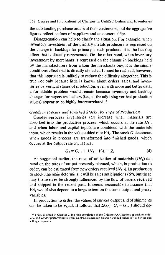
Goods in Process and Finished Stocks, by Type of ProductionGoods-in-process inventories (G) increase when materials are
absorbed into the productive process, which occurs at the rate INS,and when labor and capital inputs are combined with the materialsinput, which results in the value-added rate The stock G decreaseswhen goods in process are transformed into finished goods, whichoccurs at the output rate Hence,
= + + — (4)
As suggested earlier, the rates of utilization of materials (INs) de-pend on the rates of output presently planned, which, in production toorder, can be estimated from new orders received In productionto stock, the main determinant will be sales anticipations (Se, butthesemay themselves be strongly influenced by the flow of orders receivedand shipped in the recent past. It seems reasonable to assume that
would also depend to a large extent on the same output and proxyvariables.
In production to order, the values of current output and of shipmentscan be taken to be equal. It follows that Gg — should de-
"Thus, as noted in Chapter 7, the high correlation of the Chicago PAA indexes of backlog diffu-sion and vendor performance suggests a close association between unfilled orders of the buying andselling companies.
Orders, Production, and Inventory Investment 359
pend positively on new orders received and about to be processed andnegatively on St according to (4) and the preceding considera-tions.
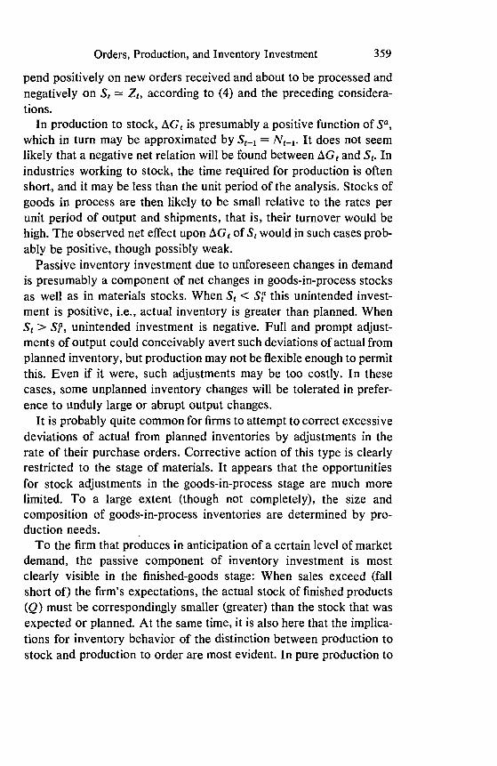
In production to stock, is presumably a positive function of S".which in turn may be approximated by = It does not seemlikely that a negative net relation will be found between and Inindustries working to stock, the time required for production is oftenshort, and it may be less than the unit period of the analysis. Stocks ofgoods in process are then likely to be small relative to the rates perunit period of output and shipments, that is, their turnover would behigh. The observed net effect upon of St would in such cases prob-ably be positive, though possibly weak.
Passive inventory investment due to unforeseen changes in demandis presumably a component of net changes in goods-in-process stocksas well as in materials stocks. When St < this unintended invest-ment is positive, i.e., actual inventory is greater than planned. When
unintended investment is negative. Full and prompt adjust-ments of output could conceivably avert such deviations of actual fromplanned inventory, but production may not be flexible enough to permitthis. Even if it were, such adjustments may be too costly. In thesecases, some unplanned inventory changes will be tolerated in prefer-ence to unduly large or abrupt output changes.
It is probably quite common for firms to attempt to correct excessivedeviations of actual from planned inventories by adjustments in therate of their purchase orders. Corrective action of this type is clearlyrestricted to the stage of materials. It appears that the opportunitiesfor stock adjustments in the goods-in-process stage are much morelimited. To a large extent (though not completely), the size andcomposition of goods-in-process inventories are determined by pro-duction needs.
To the firm that produces in anticipation of a certain level of marketdemand, the passive component of inventory investment is mostclearly visible in the finished-goods stage: When sales exceed (fallshort of) the firm's expectations, the actual stock of finished products(Q) must be correspondingly smaller (greater) than the stock that wasexpected or planned. At the same time, it is also here that the implica-tions for inventory behavior of the distinction between production tostock and production to order are most evident. In pure production to

360 Causes and Implications of Changes in Unfilled Orders and Inventories
order, no finished goods are held for sale; here Q consists only of soldproducts in transit—temporarily stored by the producer-seller or on theway to the buyer. Such stocks exist merely as a by-product of theactivity of the firms concerned; the latter do not plan investment infinished-goods inventory. For an expanding industry working to order,these stocks are likely to be growing, too, but their movements, apartfrom such trends, would probably be random or irregular.
In contrast, firms that produce for expected market demand wouldhave, as a rational goal, a desired finished-goods inventory consistentwith their sales anticipations (although, in any short unit period, theadjustment of actual Q toward the intended level may be only partial).In addition, investment in finished stocks would here probablycontain a passive component reflecting unforeseen changes in sales,as already noted.
To conclude this part of the chapter, analytical considerations sug-gest strongly that distinctions by type of production (to stock or toorder) and by stage of fabrication (materials, goods-in-process, finishedgoods) are associated with important differences in patterns and de-terminants of inventory behavior. Different models of inventoryinvestment are therefore appropriate for several different categoriesof stocks that are defined by this double classification. In much of therecent work on inventory behavior, however, the need for such dis-aggregation is not fully recognized, and attention focuses directly onaggregate inventories. A summary review of this work follows.
Recent Work on Inventory Investment:A Survey of Findings
Regression Studies of A ggre gate InventoriesThe apparently large role of inventories in postwar business cycles
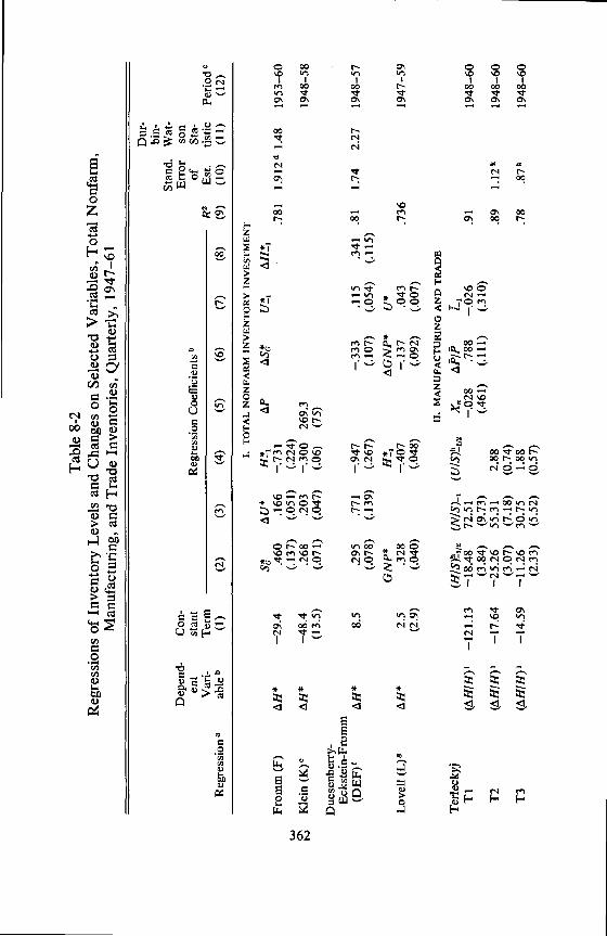
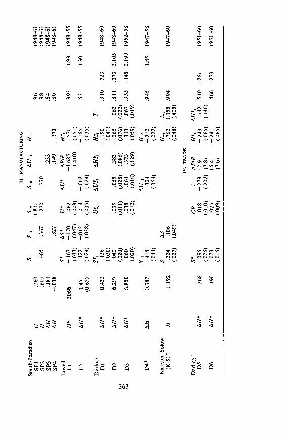
stimulated much research in this area. The output of this work consistsin large part of quarterly regressions based on comprehensive aggre-gates, and Table 8-2 assembles a large number of such estimates fromseveral published studies.16
16 Because the authors worked independently, the equations often overlap in various ways.though one could argue that some coordination of the effort would have substantially increased thenet value of the work, inferences to this effect based solely on the collected statistical results can beexaggerated: It may be more fruitful to have differing interpretations of similar relationships.

Orders, Production, and Inventory Investment 361
The table indicates a remarkable degree of consensus among thedifferent studies in the selection of the explanatory variables: The mostcommonly used are levels and changes of sales and unfilled orders.Their treatment varies mainly in that they are taken either with coin-cident timing or with different leads. Lagged inventory levels andchanges are also often included. Most of the studies are based on de-flated data but a few use current-dollar series. As a rule the data areseasonally adjusted.
Most of the equations incorporate the flexible-accelerator and buffer-stock concepts developed in earlier literature.17 Thus, common to themodels of Darling and Lovell is the basic assumption that the desired(equilibrium) inventories are a function of sales and that devia-tions between desired and actual stocks determine, with a lag, therate of inventory investment. The adjustment of inventories towardthe equilibrium level is partial in any period. However, the desiredinventory usually depends also on other variables, notably unfilledorders.
The actual stock that is compared with the desired one refers to thetime at which the decision regarding inventory investment is made; it isusually taken as of the end of the preceding (or the beginning of thecurrent) period. On this approach, the lagged inventory term will ap-pear with a negative coefficient in the inventory investment equation,but with a positive coefficient in the inventory level equation.18
In Table 8-2, the signs of the coefficients of lagged inventory are in-deed consistent with this expectation in every case (Table 8-2, part I,column 4, and parts III and IV, column 7). The coefficients are
'TThe main references here are to the work of Metzler (see note 8, above) and Richard M.Goodwin, "Secular and Cyclical Aspects of the Multiplier and Accelerator," in Income, Employ-ment, and Public Policy: Essays in Honor of Alvin H. Hansen. New York, 1948.
'8Suppose that firms, on the average, plan to eliminate in each period a fraction (8) of the dif-ference between the actual stock (H) and the anticipated desired stock (H?). The latter is a functionof anticipated sales (Sfl, which will as a rule deviate from actual sales by a forecasting error — 5).Then the intended inventory investment would depend on the discrepancy between the desired andthe actual stock, and the unintended or passive inventory investment would depend on the error ofsales anticipations:
= 8(H? — + A(S7 — + u,.
The coefficient of the previous level of stock should thus be negative (—6) in the inventoryinvestment equation, and positive (1 — 6) in the corresponding equation for the level of inventory.Cf. Michael C. Lovell, "Factors Determining Manufacturing Inventory Investment," in JointEconomic Committee, Inventory Fluctuations, Part I, p. 127; and Lovell, "Determinants of In-ventory Investment," in Models of Income Determination, Studies in Income and Wealth, Vol. 28,Princeton for NBER, 1964, pp. 179 and 194.
Tab
le 8
-2R
egre
ssio
ns o
f In
vent
ory
Lev
els
and
Cha
nges
on
Sele
cted
Var
iabl
es, T
otal
Non
farm
,M
anuf
actu
ring
, and
Tra
de I
nven
tori
es, Q
uart
erly
, 194
7—61
Dur
-bi
n-St
and.
Wat
-D
epen
d-C
on-
Err
orso
nen
tV
ail-
Reg
ress
iona
able
'1
stan
tT
erm
(1)
(2)
Reg
ress
ion
Coe
ffic
ient
s b
R2
(8)
(9)
of
Est.
(10)
Sta-
tistic
(11)
Peri
od C
(12)
(3)
(4)
(5)
(6)
(7)
I T
OT
AL
NO
NFA
RM
IN
VE
NT
OR
Y I
NV
EST
ME
NT
H!1
U!1
From
m(F
)—
29.4
.460
.166
—.7
31.7
811.
912c
1 1.
4819
53—
60(.
137)
(.05
1)(.
224)
Kle
in—
48.4
.268
.203
—.3
0026
9.3
1948
—58
(13.
5)(.
071)
(.04
7)(.
06)
(75)
Due
senb
erry
-E
ckst
ein-
From
m8.
5.2
95.7
71—
.947
—.3
33.1
15.3
41.8
11.
742.
2719
48—
57(.
078)
(.13
9)(.
267)
(.10
7)(.
054)
(.11
5)G
NP*
H!1
2.5
.328
—.4
07—
.137
.043
.736
1947
—59
(2.9
)(.
040)
(.04
8)(.
092)
(.00
7)
II. M
AN
UFA
CT
UR
ING
AN
D T
RA
DE
Ter
leck
yj(N
/S)_
113
F/P
Ti
(tiHfH)'
—12
1.13
—18.48
72.51
—.028
.788
—.026
.91
1948—60
(3.84)
(9.73)
(.461)
(.111)
(.310)
T2
—17
.64
—25.26
55.3
12.
88.89
1.12k
1948—60
(3.07)
(7.1
8)(0
.74)
T3
(tiH
fH)'
—14
.59
—11
.26
30.7
51.
88.7
8.8
7k19
48—
60(2.33)
(5.5
2)(0
.57)
III.
MA
NU
FAC
TU
RIN
G
Smith
-Par
adis
oS
S_1
S_2
S_3
AU_1
H_2
SP1
H.7
601.811
.96
1948—61
SP2
H.8
01.465
.367
.270
.770
.98
1948—61
SP3
.381
.233
.64
1948—61
SP4
—.0
38.3
27.1
49—
.173
.80
1948
—61
Lov
ell
LI
3066
.—
.167
—.1
70.0
62—
1.68
5.5
70.9
931.
9819
48—
55(.
033)
(.04
7)(.
008)
(.41
0)(.
051)
L2
—1.
47.1
22—
.012
.014
—.0
02—
.165
.53
1.30
1948
—55
(0.6
2)(.
024)
(.03
8)(.
005)
(.02
4)(.
035)
Dar
ling
S!1
H!1
TD
l—
0.43
2.1
36—
.190
.310
.723
1948
—60
(.03
0)(.
041)
D2
6.29
7.0
40.0
35.0
55.3
83—
.265
.062
.811
.373
2.10
519
48—
60(.
020)
(.01
1)(.
028)
(.08
6)(.
076)
(.02
2)D
36.850
.060
.038
.061
.373
—.313
.067
.955
.145
2.19
919
52—
58(.
020)
(.01
0)(.
018)
(.12
9)(.
059)
(.01
9)
S_1
D4'
—0.
387
.415
.324
—.2
12.9
451.
8519
47—
58(.
044)
(.05
4)(.
022)
Kar
eken
-Sol
owS
ISIS
H_1
(K-S
)tm
H—
1.19
2.224
—.106
.762
—1.
155
.994
1947
—60
(.02
7)(.
049)
(.04
8)(.
405)
IV. T
RA
DE
Dar
ling
CP
iA
P/P÷
1H
!1D
5.268
.096
.018
—.279
12.9
—.243
.142
.510
.261
1951—60
(.026)
(.01
0)(.
202)
(7.8
)(.
065)
(.14
6)D
6.1
90.0
73.0
2515
.4—
.241
.466
.273
1951
—60
(.016)
(.009)
(7.6)
(.065)
364 Causes and Implications of Changes in Unfilled Orders and Inventories
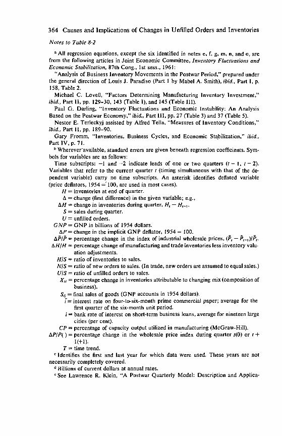
Notes to Table 8-2
a All regression equations, except the six identified in notes e, f, g, m, n, and o, arefrom the following articles in Joint Economic Committee, Inventory Fluctuations andEconomic Stabilization, 87th Cong., 1st sess., 1961:
"Analysis of Business Inventory Movements in the Postwar Period," prepared underthe general direction of Louis J. Paradiso (Part I by Mabel A. Smith), ibid., Part I, p.158, Table 2.
Michael C. Lovell, "Factors Determining Manufacturing Inventory Investment,"ibid., Part II, pp. 129—30, 143 (Table I), and 145 (Table III).
Paul G. Darling, "Inventory Fluctuations and Economic Instability: An AnalysisBased on the Postwar Economy," ibid., Part III, pp. 27 (Table 3) and 37 (Table 5).
Nestor E. Terleckyj assisted by Alfred Tella, "Measures of Inventory Conditions,"ibid., Part II, pp. 189—90.
Gary Fromm, "Inventories, Business Cycles, and Economic Stabilization," ibid.,Part IV, p. 71.
b Wherever standard errors are given beneath regression coefficients. Sym-bols for variables are as follows:
Time subscripts: —1 and —2 indicate leads of one or two quarters (t — 1, z — 2).Variables that refer to the current quarter t (timing simultaneous with that of the de-pendent variable) carry no time subscripts. An asterisk identifies deflated variable(price defiators, 1954 100, are used in most cases).
H = inventories at end of quarter.A = change (first difference) in the given variable; e.g.,
= changer in inventories during quarter, H1 —S = sales during quarter.U = unfilled orders.
GNP = GNP in billions of 1954 dollars.= change in the implicit GNP deflator, 1954 = 100. - -
AP/P = percentage change in the index of industrial wholesale prices, (P1 — P1_1)/P1.
AH/H = percentage change of manufacturing and trade inventories less inventory valu-ation adjustments.
H/S = ratio of inventories to sales.N/S = ratio of new orders to sales. (In trade, new orders are assumed to equal sales.)U/S = ratio of unfilled orders to sales.
= percentage change in inventories attributable to changing mix (composition ofbusiness).
S1 = final sales of goods (GNP accounts in 1954 dollars).T= interest rate on four-to-six-month prime commercial paper; average for the
first quarter of the six-month unit period.i = bank rate of interest on short-term business loans, average for nineteen large
cities (per cent).CP = percentage of capacity output utilized in manufacturing (McGraw-Hill).
AP/P( ) = percentage change in the wholesale price index during quarter t(0) or I +1(+1).
T = time trend.c Identifies the first and last year for which data were used. These years are not
necessarily completely covered.d Billions of current dollars at annual rates.e See Lawrence R. Klein, "A Postwar Quarterly Model: Description and Applica-
Orders, Production, and Inventory Investment 365
tions," Models of Income Deterininat ion, Studies in Income and Wealth, Vol. 28,Princeton for NBER, 1964, e.g., (6), p. 16. This equation is part of a large inter-dependent system. The method of estimation is limited information, maximum likelihood.The correlation coefficient R = .99 (stock form); it is computed as
I !Z2 T—l111 2'v T—,n
x is the dependent variable, and m is the number of parametersin the equation. Unlike elsewhere in this section, farm inventories are not excludedhere.
See James S. Duesenberry, Otto Eckstein, and Gary Fromm, "A Simulation of theUnited States Economy in Recession," Econometrica, October 1960, p. 798.
g See Michael C. Lovell, "Determinants of Inventory Investment," in Models of in-come Determination (see note e, above), equation (2.15), p. 186.
h Ratio at the beginning of the period.'Six-month changes.Three-month changes.
k Percentage points. Unbiased estimates.'See Paul G. Darling, "Manufacturers' Inventory Investment, 1947—1958," Ameri-
can Economic Review, December 1959, pp. 950—63.See John Kareken and Robert M. Solow, "Lags in Fiscal and Monetary Policy," in
Commission on Money and Credit, Stabilization Policies, Research Study One, Part I,Englewood Cliffs, N.J., 1963, equation (7), p. 43.
See Paul 0. Darling and Michael C. Lovell, "Factors Influencing Investment in In-ventories," in Duesenberry et al., eds., Brookings Quarterly Econometric Model of theUnited Stales, equations (4.12) and (4.13), p. 151.
generally rather small in absolute terms, varying from —.165 to —.407in the investment equations.t9
Reaction coefficients of 0.2 to 0.4 suggest that from about one-fifthto two-fifths of the discrepancy between desired and actual inventorywould be eliminated each quarter if no further change occurred insales (or, generally, in the determinants of the desired stocks). Thisraises a doubt and a question: Why should the adjustments of inven-tories to the desired levels be so painfully slow, resulting in such in-ordinately large unintended stocks?2° It should be remembered that
'9The two apparent exceptions are in equations F and DEF, where the estimated coefficients oflagged inventory are as large as —.731 and —.947, respectively. However, the flows are measured atannual rates here, not as absolute quarterly changes as in the other regressions; hence, thesefigures should be divided by 4 for comparability, which results in estimates of —.185 and —.195,respectively. Cf. James S. Duesenberry, Otto Eckstein, and Gary Fromm, "A Simulation of theUnited States Economy in Recession," Econometrica, October 1960, p. 796.
20See the calculated "surplus inventory" series in Lovell, "Determinants," pp. 187—88, forequation L in Part I of Table 8-2. Here, the coefficient of is on the high side of the estimates(0.407), but the surplus inventory figures are still relatively very large (most often absolutely greaterthan the corresponding values of actual inventory investment).

366 Causes and Implications of Changes in Unfilled Orders and Inventories
the estimates refer to aggregates that include not only the typicallylagging finished-goods inventories of firms selling from stock but alsopurchased materials and goods-in-process stocks, which should begeared much more closely to sales and production. These results, then,seem to me rather suspect: They could be underestimating the speed ofadjustment because of a misspecification of the determinants of the"desired" inventory.
The principal factors used as such determinants are sales and unfilledorders. They are sometimes assigned leads relative to the dependentinventory variable but are often taken as simultaneous with the latter(compare equations D1—D3 with equations Ll—L2). But actual salesare not yet known at the time when the firm decides upon the level ofits output and any desired inventory change, except in production toorder (where the known sales should be represented not by the cur-rent shipments, but by advance orders received). Hence, in principle,anticipated or ex-ante sales (Se) should be used as the main determi-nant of the desired inventory, not the actual or ex-post sales (Se). Inshort, unless sales are made in advance of production, they must bepredicted. Usually, forecasts of sales will contain errors, and these arelikely to result in some unintended or passive inventory investment.
If the forecasts were unbiased and their errors were random, arationale would exist for the use of as a surrogate measure of S?for analytical purposes; and in this case the "passive" inventory com-ponent could itself be treated as random and incorporated in theresiduals of the inventory equation.2' But there is no firm theoreticalor empirical basis for this approach. According to Nurkse, "if thecyclical variation in aggregate demand is not treated as a random per-turbation, the passive component of inventory investment cannot beeither." 22 Observations on sales anticipations are scanty, and studiesbased on them are on the whole rather inconclusive. However, even
21 approach is implicit in the inventory equation of the early aggregate model by Lawrence R.Klein (see his Economic Fluctuations in the United States, 1921—41, New York, 1950). Its logicand implications have been worked out by Edwin S. Mills in "Expectations, Uncertainty, andInventory Fluctuations," Review of Economic Studies, No. 1, 1954—55, pp. 15—23, and in "TheTheory of Inventory Decisions," Econornetrica, April 1957.
22 "Cyclical Pattern," p. 396. Nurkse recognizes that random shifts in demand from one productto another may make the passive inventory investment a random variable for individual firms orindustries. But such changes "will be in opposite directions, tending in the aggregate to cancel out.In dealing with total inventory investment, the unintended change that remains cannot be due tosuch random intercommodity shifts, but can only stem from the expansion and contraction ofdemand in the aggregate
Orders, Production, and Inventory Investment 367
the most favorable of the results obtained do not show anticipations tobe so unbiased and efficient as to justify any confident use of realizedsales as a proxy for expected sales.23
Under certain assumptions, the effect of errors in sales anticipationscould be inferred approximately from the coefficient of the change insales in the inventory equation.24 In the simple case of naive ex-pectations, = that coefficient would measure directly the frac-tion of the forecasting error that results in inventory change.25 Moregenerally, if systematic expectational errors exist and give rise topassive inventory investment, then is likely to have a significantnegative effect in inventory equations.
In Table 8-2, change-of-sales variables are included in five regres-sions; their coefficients are all negative but two are not significant (seein Part I, DEF and L; in Part III, Li, L2, and K-S). It must be remem-bered that these estimates refer to total inventories, aggregated acrosscategories with different behavioraL characteristics. The hypothesizedrelation between sales anticipation errors and buffer stocks seemsprimarily and directly applicable to finished-goods inventories; it canbe extended by analogy and implication to goods-in-process and pur-chased materials, but there it may well be much less pertinent. Moreimportant, the hypothesis is definitely limited to industries working tostock, in anticipation of market demand.
The measured effects of the backlog factor are in general strong,ranking with those of sales. For example, according to the current-
23The new quarterly OBE series on manufacturers' sales expectations apparently work betterthan some of the old (and notoriously weak) anticipations data. However, for some industries, theseseries mainly reflect information conveyed by orders received and unfilled. Generally, their effectiveforecast span is short, and their contribution to estimated models of inventory generation is neitherlarge nor well established. (See the last section of Chapter 2; also, M. C. Lovell, "Sales Anticipa-tions, Planned Inventory Investment, and Realizations," and comments by M. Hastay and R.Eisner in Determinants of Investment Behavior, Universities—National Bureau Conference 18,New York, NBER, 1967.) 1 believe the conclusion I draw in the foregoing text is a fair inferencefrom the materials presented in Albert A. Hirsch and Michael C. Lovell,SalesAnticipations and/n-ventory Behavior, New York, 1961.
24This will be so, for example, if the anticipated sales change represents a fraction of the actualchange and the effects of current output and price adjustments are separately estimated or assumedto be negligible. See Lovell, "Determinants," pp. 203—204.
25 Suppose that = a + By substitution into the equation shown in note 18, above, one gets
Ba + (8/3 + — — +
If = S,_1, this is equivalent to
= Ba + 813S,_1 — X(S1 — — BHr_i + U,.
If + v1, where v1 is random (as in the studies referred to in note 21), then
— Ba + 8/35, — BH,_1 + (6/3 + X)v1 + u,.
368 Causes and Implications of Changes in Unfilled Orders and Inventories
dollar estimates SP3 and SP4, the change in manufacturers' unfilledorders alone accounts for 64 per cent of the variance in manufacturers'inventory investment in 1948—61; the addition of the prior sales changeand inventory level raises this proportion to 80 per cent. In anotherstudy using deflated variables, a regression of inventory investment onprior sales change and inventory level yielded an R2 of only .310, andthe addition of the unfilled orders variables U* and plus aratchet term and trend factor, raisedR2 to .811 (equations Dl and D2).The role of unfilled orders is also important in the regressions for totalor nonfarm inventory investment and for manufacturing and tradeinventories combined (all the equations in Part I of Table 8-2 and, also,equations T2 and T3).26
The aggregative backlog-inventory relationship, although highlysignificant statistically, does not tend itself to a straightforward analyti-cal interpretation. Since unfilled orders of sellers are also outstandingorders of buyers, their rise may stimulate inventory investment ofbuyers as well as sellers in two different ways. Aggregation overstages of fabrication provides still another source of difficulty. An in-crease in unfilled orders is likely to stimulate buying of materials bythose who are to fill the orders, but it will hardly be associated with anincrease in the finished stocks of these producers. On the contrary,where backlogs accumulate so that production may be order-oriented.the need for finished inventory is reduced.
Other variables received considerably less attention and yieldedresults that seem partly negative but should probably be regardedrather as inconclusive. Lovell found no support for the hypothesis thatactual price increases, by creating expectations of price rises, stimulateinventory investment; actually, the coefficient of in his equationLi is negative. Darling did obtain positive coefficients for his proxyfor price expectations (the proportionate change in the wholesaleprice index during the approaching quarter) in his study of trade inven-tories (equations D5 and D6).27 One possible explanation for the nega-tive results in the manufacturing equations is that the effect of the
26 In the T equations, unfilled orders are used in the form of a ratio to sales. Also included is theratio of new orders to sales, which is highly correlated with the chinge in unfilled orders. Terleckyjassumes that unfilled orders in trade are nil. His results raise a difficulty concerning the influenceof sales (see Lovell, "Determinants," p. 185).
27 Terleckyj also reports a significant positive coefficient for the concurrent relative change inthe industrial price index, but not for the prior change. The use of undeflated data in his study mightbe an appreciable drawback in this context.

Orders, Production, and Inventory Investment 369
price change could not be separated from that of the change in unfilledorders. However, Klein reports significant positive associations be-tween aggregate inventory investment and changes in both the GNPprice deflator and unfilled orders (the price variable being taken with-out and the backlog variable with a lead; see equation K).
The Kareken-Solow equation based on undeflated data for manu-facturing includes the interest rate on short-term bank loans to businesswith a significant coefficient that has the expected negative sign anddenotes a small (—0.4) elasticity at the point of the means. The evi-dence on the effects of interest rates and liquidity factors assembledby McGouldrick is mixed and not encouraging.28 In contrast to thesestudies, more promising indications of the role of financial variables ininventory determination are reported by Ta-Chung Liu29 and Paul W.Kuznets.3°
Major-industry and Stage-of-Fabrication EstimatesDisaggregation by industry and stage of fabrication is not a frequent
feature of regression studies of inventory behavior. Furthermore, dis-aggregation has for the most part been used in a very limited sense, withthe same or very similar models being applied to the different sectors orcategories of stocks.
Table 8-3 shows some further results of Lovell's 1961 study.31 These
Paul F. McGouldrick, "The Empact of Credit Cost and Availability on Inventory Invest-ment," in Joint Economic Committee, Inventory Fluctuations, Part II, pp. 89—117.
2°"An Exploratory Quarterly Econometric Model of Effective Demand in the Postwar U.S.Economy," Econunietrjca, July 1963, pp. 301—48. Liu uses a real-interest variable, defined as thedifference between the average rate on prime commercial paper (4—6 months) and the lagged rateof change in the GNP price deflator, both in per cent per year, Its coefficient is about—0.3, with astandard error half as large. Interestingly, Liu's equation also includes, among others, money andtime deposits held by nonfarin nonfinancial business (in constant dollars). This variable has apositive coefficient, which, however, is small relative to its standard error, according to simple leastsquares (the two-stage estimate is more significant).
"Financial Determinants of Manufacturing Inventory Behavior: A Quarterly Study Based onUnited States Estimates, 1947—1961," Yale Economic Essays, Fall 1964, pp. 331—69. The equationthat presents the financial variables in the best light reads:
= —953.3 + .088S, ± + 1.07 11F1_, + .1 I4XF1_, — I 5.6i1_, ± .737H,_1,(.018) (.010) (0.253) (.028) (7.2) (.049)
where the data are for all manufacturers, in constant (1954) dollars. IF and XF denote internal andexternal finance, respectively, and I is the average interest rate for short-term business loans. Each ofthe three financial variables is here transformed according to a moving average formula with triangu-lar weights that implies rather extended (seven-quarter) adjustment periods. When these variablesare entered with simple one-period lags (in an equation which contains the same nonfinancial vari-ables, including H1_,), the coefficients of and !F1_, are apparently not significant. On the otherhand, the other variables require no transformation, and their effectiveness seems to be relativelyindependent of the different specifications of the financial factors (ibid., Table 1, p. 352).
" In Inventory Fluctuations, Part II. This is also the source of equations LI and L2 in Table 8.2.

Tab
le 8
-3R
egre
ssio
ns o
f In
vent
ory
Lev
els
and
Cha
nges
on
Sele
cted
Var
iabl
es, T
otal
Inv
ento
ries
, Pur
chas
ed M
ater
ials
and
Goo
ds in
Pro
cess
, and
Fin
ishe
d-G
oods
Inv
ento
ries
, All
Man
ufac
turi
ng a
nd M
ajor
-Ind
ustr
y G
roup
s,19
48—
55 a
nd 1
948—
60
Dur
bin-
Wat
son
Dep
ende
ntC
onst
ant
Sta-
Indu
stry
Var
iabl
eT
erm
Reg
ress
ion
Coe
ffic
ient
sR
2tis
tic
PUR
CH
ASE
D M
AT
ER
IAL
S A
ND
GO
OD
S IN
PR
OC
ESS
U'
(M+
G)!
11.
All
mfg
.(M
+ G
)*40
04.0
62—
.100
.061
—.3
20.5
42.9
932.
27(.
016)
(.03
0)(.
005)
(.20
6)(.
046)
2. D
urab
les
(M+
G)*
1412
.053
—.0
80.0
38.0
38.6
37.9
941.
82(.
019)
(.03
0)(.
004)
(.17
3)(.
034)
3. N
ondu
rabl
es(M
+ G
)*—
356
.023
—.0
37.2
21.1
48.9
03.9
702.
02(.
021)
(.05
6)(.
051)
(.12
1)(.
067)
FIN
ISH
ED
-GO
OD
S IN
VE
NT
OR
IES
s*4.
All
mig
.Q
*—
258
.042
.132
.848
.958
1.39
(.02
0)(.
042)
(.06
5)5.
Dur
able
sQ
*—
326
.055
.097
.817
.966
1.33
(.01
4)(.
028)
(.05
2)6.
Non
dura
bles
419
.006
.170
.935
.947
1.57
(.02
9)(.
068)
(.08
6)

TO
TA
L I
NV
EN
TO
RIE
S (L
EV
EL
OR
CH
AN
GE
S)
7. D
urab
les
H*
1032
..1
26.1
04.0
37—
.499
.676
.991
1.46
(.03
7)(.
054)
(.00
6)(.
331)
(.04
5)8.
Dur
able
s—
1.55
.127
—.0
02.0
09.0
47—
.115
.57
1.23
(0.5
5)(.
033)
(.04
4)(.
005)
(.02
1)(.
033)
9. N
ondu
rabl
es—
661.
.036
.171
.329
—.6
18.9
26.9
812.
23(.
038)
(.07
5)(.
083)
(.18
5)(.
065)
10. N
ondu
rabl
es—
0.50
8.0
43—
.029
.254
—.3
56—
.082
.66
1.93
(0.4
09)
(.01
6)(.
033)
(.04
6)(.
058)
,(.
039)
11. P
rim
ary
met
als
11*
—17
2.8
.063
.043
.018
—.0
36.9
45.9
391.
72(.
03 1
)(.
032)
(.01
2)(.
035)
(.05
3)12
. Mac
hine
ry75
1.9
.035
.070
.059
.029
.701
.991
1.49
(.03
9)(.
065)
(.00
7)(.
067)
(.04
3)13
. Tra
nspo
rt. e
quip
.26
6.0
.083
.031
.032
.006
.684
.990
1.13
(.03
2)(.
046)
(.00
5)(.
084)
(.05
4)14
. Sto
ne, c
lay,
and
gla
ss27
.4.1
08.2
34a
.002
.733
.978
1.29
(.02
0)(.
050)
(.02
0)(.
051)
15. O
ther
dur
able
s32
.8.1
22.1
35a
a.8
06.9
600.
92(.
030)
(.04
8)(.
050)
Not
e: S
ee T
able
8-2
, not
e b,
for
exp
lana
tion
of a
ll sy
mbo
ls e
xcep
t the
fol
low
ing:
M =
purc
hase
dm
ater
ial i
nven
tori
es.
G =
good
s-in
-pro
cess
inve
ntor
ies.
Q=
fini
shed
-goo
dsin
vent
orie
s.Z
S +
tXQ
=va
lue
of o
utpu
t est
imat
ed b
y ad
ding
cha
nge
in f
inis
hed-
good
s in
vent
ory
to s
ales
.So
urce
: Mic
hael
C. L
ovel
l, "F
acto
rs D
eter
min
ing
Man
ufac
turi
ng I
nven
tory
Inv
estm
ent,"
in J
oint
Eco
nom
ic C
omm
ittee
, Inv
ento
ryFl
uctu
atio
ns a
nd E
cono
mic
Sta
biliz
atio
n, 8
7th
Con
g., 1
st s
ess.
, 196
1, P
art I
I. E
ntri
es o
n lin
es 1
—3
are
from
Tab
le 1
, P. 1
43; l
ines
4—
6, f
rom
Tab
le I
I, p
. 144
; and
line
s 7,
9, a
nd 1
1—15
, fro
m T
able
111
, p. 1
45. A
ll th
ese
regr
essi
ons
are
base
d on
def
late
d, s
easo
nally
adj
uste
d, q
uart
erly
seri
es f
or 1
948—
55. E
ntri
es o
n lin
es 8
and
10
are
from
equ
atio
ns g
iven
in ib
id.,
pp. 1
29—
30; t
hey
refe
r to
qua
rter
ly d
efla
ted
and
dese
ason
aliz
edda
ta f
or 1
948—
60.
aLa
ckof
dat
a is
cite
d as
the
reas
on f
or a
bsen
ce o
f es
timat
es in
thes
e ce
lls.

372 Causes and Implications of Changes in Unfilled Orders and Inventories
regressions use largely simultaneous relationships between constant-dollar series. Only one of the explanatory variables is taken with alead: the inventory level as of the end of the previous quarter,However, no account is taken of the possible feedback effects of inven-tory investment on sales, unfilled orders, etc., that could impose asimultaneous equation bias on the estimates.
One model, based on the flexible or partial-adjustment version ofthe acceleration principle, is adopted for both the purchased-materialsand goods-in-process inventories (first three lines). The desired level ofthe combined inventory for these two stages is assumed to be a linearfunction of the level of output, the change in output, unfilled orders, andthe relative change in the wholesale price index. Realized inventoryinvestment, + is viewed as a fraction, 8, of the differencebetween the desired and the available stock. Since the dependentvariable is the level of inventory, its previous value, (M + hasthe coefficient (1 — 8).
The sign of the coefficient of the change in output is not clearlyprespecified. "When output is increasing, orders may be placed withsuppliers in an attempt to build up stocks, but considerable delays maybe involved in obtaining delivery."32 On this reasoning, the effect of
would be positive if the attempt succeeded. Negative estimatedcoefficients would then be attributed to long delivery lags for materials.But the evidence reviewed earlier in this chapter suggests that thedelivery lags for materials are on the whole rather short. A differentexplanation of the negative effect of is that this term, being wellcorrelated with reflects the influence of sales anticipation errorsin production to stock: After all, passive or unintended changes due tosuch errors can occur in purchased-materials and goods-in-processinventories as well as in finished-goods stocks. Of course, unexpecteddelivery delays may here and there also contribute to the observedresults.
The model appears to work poorly for the nondurable goods sector,where the estimates are unsatisfactory or implausible. The coefficientsof Z*, and iSP/P are all small relative to their standard errors,and the reaction coefficient 6, computed as I minus the coefficient oflagged inventory, is very small indeed (0.097). Of the causal variables,
32 ibid., p. 140.
Orders, Production, and Inventory Investment 373
only unfilled orders, which in this sector are assumed to be nil for mostindustries and of modest size for a few (according to the statisticsused), have a significantly large positive coefficient (Table 8-3, thirdline). The results for all manufacturing and the durable goods sectorare considerably better, since Z* and as well as U*, show signifi-cant effects, while the estimates for6 are much larger and more reason-able (0.458 and 0.363, respectively). However, the evidence on theinfluence of price changes is again negative.
In the finished-goods inventory equations, a simple form of the"buffer-stock motive" is adopted and neither U* nor is included.Deflated sales, not output, are now used. The influence of S7 is posi-tive and significant for all manufacturing and the durable goods in-dustries, but it is not significant for the nondurables. The coefficients of
are large relative to their standard errors in each case, but theyare positive. If these coefficients were to represent the effects of salesanticipation errors that result in passive or unintended inventorychanges, their signs ought to be negative. On Lovell's more complexinterpretation, however, these estimates must be "unscrambled" toreveal the implicit "anticipation coefficient," p."
One would expect the adjustments of finished-goods inventories tobe slower than those of the materials and goods-in-process inventories.The coefficients of are much higher than those of (M + inTable 8-3, which is, in terms of the model applied here, consistent withthis expectation. But the implied reaction coefficients of 0.152 for allmanufacturing, 0.183 for the durables, and 0.065 for the nondurablesseem uncomfortably low. The large coefficients of reflect the highautocorrelations of the smooth series on aggregate finished-goodsstocks, and probably also reflect the limitation of these equations totwo causal variables (S* and only; it is not at all clear that theycan be safely used to infer extremely low reaction coefficients, i.e.,extremely slow inventory adjustments.
Defining = p = I for naive or static expectations (Si' =and p = 0 for unbiased expectations (S' = Se). On this definition, the coefficient of equals(8/3+ X)p (see notes 18 and 25, above, on the meaning of6, /3, and A). The model does not providesufficient information to permit unconstrained simultaneous estimation of both A and p. If one as-sumes that A = I (complete inflexibility of production plans), p varies from 0.092 for the durablesto 0.168 for the nondurables. The implication would be that manufacturers' sales forecasts arerather good, particularly in the durable goods sector. If moderately large output adjustments wereassumed, the estimates of p would be larger, but still not very high (given A = 0.5, for example, pfor all manufacturing would be 0.243, instead of 0.126, obtained when A I).
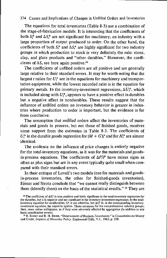
374 Causes and Implications of Changes in Unfilled Orders and Inventories
The equations for total inventories (Table 8-3) use a combination ofthe stage-of-fabrication models. It is interesting that the coefficients ofboth and are not significant for machinery, an industry with alarge proportion of output produced to order. On the other hand, thecoefficients of both and are highly significant for two industrygroups in which production to stock is very definitely the rule: stone,clay, and glass products and "other durables." However, the coeffi-cients of are here again positive.34
The coefficients of unfilled orders are all positive and are generallylarge relative to their standard errors. It may be worth noting that thelargest t ratios for are in the equations for machinery and transpor-tation equipment, while the lowest recorded ratio is in the equation forprimary metals. In the inventory-investment regressions, whichis included along with appears to have a positive effect in durablesbut a negative effect in nondurables. These results suggest that theinfluence of unfilled orders on inventory behavior is greater in indus-tries where production to order is important, but the evidence is farfrom conclusive.
The assumption that unfilled orders affect the inventories of mate-rials and goods in process, but not those of finished goods, receivessome support from the estimates in Table 8-3. The coefficients ofU7 in the durable goods regression for (M + and for are almostidentical.
The evidence on the influence of price changes is entirely negativefor the total-inventory equations, as it was for the materials and goods-in-process equations. The coefficients of IXPIP have minus signs asoften as plus signs but are in any event typically quite small when com-pared with their standard errors.
In their critique of Lovell's two models (one for materials and goods-in-process inventories, the other for finished-goods inventories),Eisner and Strotz conclude that "we cannot really distinguish betweenthem (identify them) on the basis of the statistical results." They are
coefficient is also positive and fairly significant in the total-inventory regression forthe durables, but it is negative and not significant in the inventory investment regression. In the total-inventory equation for nondurables, S," is not effective, but is; in the corresponding inventory-investment equation, the opposite applies. These estimates for the comprehensive industry groups,then, seem rather ambiguous, as if they were adversely affected by aggregation (in addition to anybasic specification errors).
R. Eisner and R. H. Strotz, "Determinants of Business Investment," in Commission on Moneyand Credit, I,npacts of Monetary Policy, Englewood Cliffs, N.J., 1963, p. 220.

Orders, Production, and Inventory Investment 375
not persuaded that inventories should be disaggregated by stage offabrication and state their preference to "disaggregate by motive"(ibid., p. 106). But motivations, here as elsewhere, must be analyzedwithin the context of the relevant technological and institutional con-straints.36 If my observations are correct, Lovell's results suffer frominsufficient rather than from excessive disaggregation (as well as fromsome errors of specification). It is important for the analysis of inven-tory behavior to distinguish between production to stock and produc-tion to order, and among the stages of fabrication, and to combinethese distinctions.
Disaggregation by Type of ProductionThomas J. Courchene has recently made a very interesting examina-
tion of several hypotheses relating to the central proposition that inven-tory behavior differs significantly between industries producing largelyto stock and industries producing largely to order, depending at thesame time also on the stage of fabrication at which the stocks areheld.37 Courchene computed inventory investment regressions for tendivisions of Canadian manufacturing that are broadly similar to theU.S. data for the "market categories." Particularly interesting, andemphasized, are his estimates for two sectors in which inventory poli-cies are governed by demand rather than supply conditions: (1) heavytransportation equipment (HTE), where production is almost exclu-sively to order; and (2) semidurable consumer goods (SDCG), whereproduction to stock definitely predominates.38
Courchene's main results for these two sectors are reproduced inTable 8-4. Application to extremes should bring out the hypothesized
'6The motives for investment and their implications certainly form an important subject to bestudied with the aid of economic theory, whether it is investment in inventories or in other capitalgoods such as structures and equipment; but so are the above-noted "constraints." Now, in thecase of inventories, these underlying conditions are quite different for, say, investment in materials(which are inputs into the production process) and finished goods (which, for the investing firm,are the outputs). Such distinctions, therefore, may be as important as those by motives, even froma purely theoretical point of view.
Courchene, "Inventory Behaviour and the Stock-Order Distinction: An Analysis by Industryand Stage of Fabrication with Empirical Application to the Canadian Manufacturing Sector,"Canadian Journal of Economics and Science, August 1967, pp. 325—57.
Applying the criterion of the stock-backlog ratios Q/U (as discussed in Chapter 2 above),Courchene presents a "ranking of sectors along [a] stock-order spectrum." Classified as producingprimarily to order are heavy transportation, other capital goods, and construction goods, while in-termediate goods and supplies, motor vehicles, "largely export producing," and semidurable andperishable consumer goods, are found to represent primarily manufacture to stock. The durableconsumer goods sector is treated as mixed.
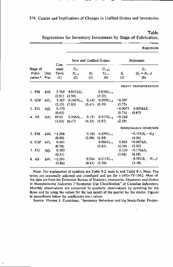
376 Causes and Implications of Changes in Unfilled Orders and Inventories
TableRegressions for Inventory Investment by Stage of Fabrication,
Stage ofCon-stant
Regression
New and Unfilled Orders Shipments
U1; U1_2; S1;
Fabri- Dep. Term N1_1 N1 U,_1 S1 (S1 — N1_1)cation a Var. (1) (2) (3) (4) (5) (6)
HEAVY TRANSPORTATION
1. PM 2.765(2.91) (3.90)
O.038U1_1
(3.52)2. GIP 5.363
(2.15)0.241N1_1
(7.83)0.142 0.295U1_2(5.41) (8.19)
—0.307(3.75)
3. FG 0.170(0.65)
—0.0075(0.73) (0.87)
4. All 10.62(3.03)
0.266N1_1(6.17)
0.151 0.317U1_2(4.35) (5.97)
—0.280(2,59)
SEMI DURABLE CONSUMER
5. PM —1.266(0.80)
0.165 0.159U1_1(3.98) (2.84)
—0.193(S1—N1)(4.06)
6. GIP 0.401(0.78)
0.066U1_1(3.81)
0.063(4.39) (3.03)
7. FG 0.202(0.33)
0.130(3.66) (4.18)
8. All —2.291(0.86)
0.264 0.217U1_1(4.41) (2.36)
—0.381(S1 — N1_1)
(5.18)
Note: For explanation of symbols see Table 8-2, note b, and Table 8-3, Note. Theseries are seasonally adjusted and undeflated and are for I-1955—IV-1962. Most ofthe data are from the Dominion Bureau of Statistics, Inventories Shipments and Ordersin Manufacturing Industries ("Economic Use Classification" of Canadian industries).Monthly observations are converted to quarterly observations by summing for theflows and by using the values for the last month of the quarter for the stocks. Figuresin parentheses below the coefficients are r values.
Source: Thomas J. Courchene, "Inventory Behaviour and the Stock-Order Distinc-
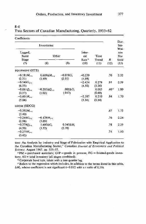
Orders, Production, and Inventory Investment 377
8-4Two Sectors of Canadian Manufacturing, Quarterly, 1955—62
CoefficientsDur-bin-Wat-son
Inventories
Inter-Lagged,Same OtherStage
(7) (8)
estRate b
(10)
TimeTrend(11)
R(12)
Sta-tistic(13)(9)
EQUIPMENT (HTE)
—0.181M1_1 —0.078G1 —0.239 .70 2.32(2.31) (3.49) (2.95) (1.99)
—2.434 0.278 .91 2.39(6.55) (4.50) (5.26)
—0.061Q,_1 0.003 .40c 1.80(0.37) (1.02) (.017) (0.68)
—0.601H1_1 —2.387 0.210 .84 1.70(5.04) (3.34) (3.14)
GOODS (SDCG)
—0.392M1_1 .67 1.73(3.40)
—0.244G1...1 .76 2.24(2.98) (3.69)
O.345AM1 .78 2.29(4.50) (3.52) (2.70)
.75 1.50
(3.42)
tion: An Analysis by Industry and Stage of Fabrication with Empirical Application tothe Canadian Manufacturing Sector," Canadian Journal of Economics and PoliticalScience, August 1967, pp. 325—57.
a PM = purchased materials; GIP = goods in process; FG = finished-goods inven-tory; All = total inventory (all stages combined).
b Corporate bond rate, taken with a one-quarter lag.c Refers to the regression which includes, in addition to the terms listed in this table,
whose coefficient is not significant (—0.012 with a t ratio of 0.19).
378 Causes and Implications of Changes in Unfilled Orders and Inventories
differences in inventory behavior most forcefully, but comparisonsbetween other sectors in which either type of production prevailsshould also show such differences, although in a more attenuated form.The evidence confirms this expectation in large part. Limitations ofthe available data, however, seriously impede the analysis and alsoits evaluation.39
The basic approach is once more guided by the familiar flexible-accelerator hypothesis. Intended inventory investment is a fraction ofthe difference between the desired and the available stock. A negativecoefficient of the lagged inventory term is therefore expected. Its abso-lute magnitude is viewed as an estimate of the above fraction. Thesecoefficients are shown in column 7 of Table 8-4; they are all negativeand significant, except for the coefficient of in the finished-goodsequation for the HTE sector, which is not significant.
The main differences in inventory behavior between production tostock and production to order derive from differences in (1) the rolesof new orders and shipments as determinants of planned output andinventories; (2) the significance of passive or unintended inventoryinvestment; and (3) the nature and function of finished-goods inven-tories.
1. In the HTE sector, representing manufacture to order, previousvalues of unfilled orders (Ug_2) are important factors in the purchased-materials and goods-in-process equations (Table 8-4). Large backlogsindicate high levels of future output, hence greater materials require-ments for production. It is also possible that, when backlogs of orderaccumulate, buying of materials would be accelerated because ofexpected delays on the suppliers' deliveries.40 Goods-in-process stockstend to be closely related to the role of production, which is herelargely determined by the amount of new orders received in the past;but output is made less volatile than new orders because backlogs actas a buffer. Hence depends positively on prior values of new and
quarterly series used cover only eight years, 1955—62. Corresponding price data are notavailable, and the series are not deflated. Sales anticipations are not directly measured but areequated to the preceding values of shipments or new orders, thus implying that a naive model ofcurrent-level extrapolation adequately represents the expectational process involved. The validityof the concept of materials ownership and the need for data on orders placed are recognized, butthe manufacturing statistics for Canada (like those for the United States) refer only to orders re-ceived and unfilled, not to orders placed and outstanding.
40 Here it would be more appropriate to use the unfilled orders of the materials suppliers as anindicator, rather than the unfilled orders of the purchasers, but data are available only for the latter.

Orders, Production, and Inventory Investment 379
unfilled orders, with some sizable lags reflecting the time-consumingnature of the production process involved (second line).
Stocks of materials are increased through deliveries on purchaseorders and decreased through transformation into stocks of goods inprocess [see equation (1), above]. The regression for in the firstline includes the stock of goods in process, which has a significantnegative coefficient, thus roughly isolating the effect of the rate of thistransformation (i.e., of the use of materials as productive inputs, iN1).
Stocks of goods in process are increased through inflow of materialsand decreased through outflow into the finished-goods stocks [equa-tion (4), above]. The rate of this outflow is measured by the rate ofoutput or (in production to order) of shipments. Hence, àG1 should benegatively related to S1, and it is (second line).41
In the SDCG sector, representing manufacture to stock, elements ofproduction to order nevertheless exist, as indicated by the presence ofunfilled orders which, although relatively small, have significant effectson and (see fifth and sixth lines, column 4). However, thelags are shorter, and the importance of the backlog factor (as indicatedby the t ratios) is smaller for the SDCG sector than for the HTE one.
Since the production process is typically short for SDCG, it is notpossible here to distinguish between the inflow and outflow factors inthe purchased-materials and goods-in-process regressions. The turn-over ratios of quarterly shipments to product inventory are high—greater than I —in this as in other sectors producing primarily to stock.New orders or shipments (the two do not differ much) appear withpositive signs in the SDCG equations for LXM1 and (fifth and sixthlines, columns 3 and 5).
2. Sales anticipations that guide production in industries working tostock inevitably generate errors, and so passive inventory investmentdue to these errors is a feature of these industries. As an illustration,the coefficients (column 6) of or of (S1 — N11) are all negative andhighly significant for the SDCG sector. Where production is under-taken in response to demand (past orders from customers), rather than
Note that the coefficient of S1 is also negative in the total inventory investment equation forHTE (column 5). This can only be explained in production to order; in production to stock, theeffect of S, is positive (see text below), and it is usually presumed to be so in aggregate inventoryanalyses. Courchene also reports that for total Canadian manufacturing, the coefficient of S1 inthe equation for AG1 is insignificant, because of offsetting effects in the two types of production(ibid., pp. 3 43—44).
380 Causes and Implications of Changes in Unfilled Orders and Inventories
in anticipation of demand (future market sales), there is clearly nobasis for such an association between forecasting errors and inventorychanges. The coefficient of LiS, in the finished-goods equation for theHTE sector is therefore not significant, as would be expected (thirdline). Sales forecast errors may influence purchases of materials byindustries producing to order, but it is difficult to isolate this effect inregressions for net change in materials stocks (where purchase ordersfor materials are not separately observed or analyzed).
3. Stocks of finished goods are small in the HTE sector, representingmainly sold output in transit to the buyer. Changes in such stocksshould be largely random, due to occasional shipping delays and per-haps cancellations (but the latter are not likely to be very frequent inthis late stage of production), although some upward trend could arisehere for a growing industry. In fact, the flexible-accelerator hypothesisthat seems to work rather well elsewhere fails entirely in the HTEequation for finished-goods inventories (Table 8-4). None of the regres-sion coefficients here is unambiguously significant, and the signs ofsome (those of and are contrary to expectations. Only 16 percent of the variance of is accounted for by the equation.
In contrast, the behavior of finished-goods inventories in the produc-tion-to-stock sector SDCG conforms well to the hypothesis in terms ofthe signs and significance of the coefficients of S1, and Inparticular, the coefficient of iXS1 is here negative and larger absolutelythan the (positive) coefficient of S1. This indicates that passive inven-tory investment plays a large role in this case and that there are im-portant elements of an inverse relation in the movements of Qt and
To conclude this review, the evidence presented does indeed con-firm the existence of systematic and important differences in inventorybehavior between production to stock and production to order. Thedifferences between stages of fabrication also become more significantwhen the distinction between the two types of operation is taken intoaccount. These results are not altered by the inclusion in the analysisof some other factors that are apparently much less important as de-terminants of inventory investment than the orders and shipmentsvariables.42
42 Interest rates are the most important of these factors in Courchene's study. The expectednegative effects of interest rates are reported in several of his regressions. In addition to the short-term rates more commonly used in inventory analysis, long-term (corporate bond) rates were usedwith similar results.

Orders, Production, and Inventory Investment 381
The Supporting Equations for Orders in RecentModels of the Economy
To the extent that new and unfilled orders are included in the com-prehensive econometric models, their main function is to contribute tothe explanation of inventory changes. Their treatment here is typicallyrather ad hoc and cursory; they are presumptive tools, not objects ofinterest in their own right. Nevertheless, as endogenous variables insystems of simultaneous equations, orders must themselves be "ex-plained," which introduces a source of potentially important errors(the more so, the greater the role of orders in determining inventoryinvestment and the greater the effects of inventory investment on theshort-run fluctuations of the economy at large).
Gary Fromm's quarterly model (1962) includes the following esti-mated unfilled orders function:
111.4— +(.109) (.332) (.104) (.101)
Fromm proceeds from the identity N1 — SI, but his use of GNPfinal sales, as if it were substitutable for S1 (the much smaller manu-facturers shipments) is at least doubtful. He also uses the definition of
U to argue that the coefficient of S$ should be negative, but this againis questionable for the same reason. (Moreover, one could maintainthat the effect of in the above equation is actually positive, thoughsmall.)
In the 1964 model by Lawrence Klein, unfilled orders are a functionof new orders and the rate of capacity utilization computed from GNPdata. The equation,45 estimated by two-stage least squares, reads
+2.12N1+(44) (0.84) (55)
"Inventories, Business Cycles, and Economic Stabilization," in Joint Economic Committee,Inventory Fluctuations, Part LV. Some symbols have been changed to conform to the notations usedelsewhere in this book: denotes final sales of goods in period t(GNP component), and U1 denotesmanufacturers' unfilled orders at the end of period 1, both in 1954' dollars; A stands for quarterlychanges.
44Fromm lets N1 = a + PS?, with /3 < 1, then states that, since AU1 —5?, txU1 a +(/3— 1)
(ibid., p. 73, n. 38). But AU1 is not identically equal to (N1 — Se); it equals (N1 — S1), and S1 cer-tainly differs from As for the estimates reproduced in the text, note that the terms +.523AS? may be rewritten as .135SV —
Lawrence R. Klein, "A Postwar Quarterly Model" in Models of Income Determination (seealso Table 8-2, equation K).

382 Causes and Implications of Changes in Unfilled Orders and Inventories
where X is private gross national product, is estimated privateGNP at full capacity, and all variables are expressed in billions of1964 dollars. Since changes in backlogs reflect the varying pressure ofdemand upon capacity, it is well to find that U is positively related toan independent measure of such pressures, namely, the ratio Re-lating the simultaneous values of U and N, however, does not result ina very adequate or interesting specification.46
An additional equation is then required to explain new orders, andthe variables employed by Klein for this purpose are recent "sales ofprivate GNP" (i.e., X — where is inventory investment in billionsof 1954 dollars) and recent change in prices (more precisely, in p, theimplicit GNP deflator, 1954 = 1.00). The equation, estimated by thelimited-information maximum-likelihood method, reads
= 2.56 + .059(X — + — Pt—i).(3.2) (.010) (72.0)
The dependence of new orders on recent price changes is certainlyof considerable interest. It could mean that price expectations areformed by projecting past changes, and that attempts to "beat the pricehike" and to "wait for better buys" lead to increased ordering after arise in p and to decreased ordering after a fall in p. But another argu-ment that is relevant at this point was developed in Chapter 7. Pricechanges are correlated with backlog changes, and the latter lead neworders.47
The relationship between new orders and recent "sales," definedbroadly as X — may represent an important link in the propagationof demand. However, new orders turn earlier than GNP; so this con-nection is not likely to be of much help in explaining the tendency ofnew orders to lead at recessions and revivals in aggregate economicactivity. The exclusion of the government component from the "sales"variable could be questioned, since includes defense and other gov-ernment orders.
The Brookings model in its first version (1965) is similar to othersin basing the inventory investment equations on a stock adjustment
Since U, by definition, equals the cumulated total of past differences between N and S, it shouldbe positively associated with and negatively associated with presumably with weights de-clining with the increasing lags 1.
The relation between prices and unfilled orders is actually used in some of the equations de-signed to explain specific price levels in Klein's model. See Chapter 7, note 52, above and the textdiscussion thereto.

Orders, Production, and Inventory Investment 383
process, with GNP "final sales" components and manufacturers' un-filled orders cast as the principal explanatory variables.48 Lagged valuesof levels and changes in unfilled orders are used, but in most cases theGNP sales terms coincide in timing with the inventory variables. Thereis disaggregation by production sector (durable manufacturing, non-durable manufacturing, trade, and other), and orders are included inthe manufacturing relations only. The model accordingly containsfunctions for new and unfilled orders in each of the two manufacturingsectors, which adds up to four equations.
Disaggregation in the form used in the Brookings model hurts ratherthan helps some of these equations when orders and sales are takenwith simultaneous timing, because of the interaction between thesevariables. For example, new orders for durable goods are regressedon the GNP component representing final sales of durables plus newconstruction. But expenditures follow orders; when the two are takenfor the same quarter, it is presumably more appropriate to say thatorders determine expenditures than to specify the reverse. A similarform is used for nondurables, where the delivery periods tend to beso short that orders are likely to reflect transactions which are alsocontained in the nondurable goods component of GNP. Some of theunderlying industry equations developed for the Brookings project byManoranjan Dutta49 similarly include the gross product originating inthe given industry, which again is more a consequence than a sourceof new orders received by the same group of firms in the same quarter.These specifications seem to have been devised for orders placed, notfor orders received, by the given industry; yet, except for the economyas a whole, the two concepts differ and the available series refer toorders received only.5°
In short, final sales of durables and nondurables can hardly be viewed
48 Gary Fromni arid Lawrence R. Klein, "The Complete Model: A First Approximation," inJ. S. Duesenberry, 0. Fromm, L. R. Klein, and E. Kuh, eds., The Brookings Quarterly EconometricModel of the United States, Chicago-Amsterdam, 1965, pp. 688—89 and 723.
"Business Anticipatory Demand: An Analysis of Business Orders, 1948—1962," in Duesenberryet al. (eds.), The Brookings Mode!, pp. 162—75.
'° As Dutta states: "Taking an aggregative view of the production sectors of the economy, ordersreceived and orders placed reduce to the same economic magnitude. This generalization has been amaintained hypothesis of this study" (ibid., p. 175). Dutta's equations for the following industriesare open to the criticism given in the text above: electrical machinery (one of the alternative formsoffered); transportation equipment, total; motor vehicles and parts; and lumber, furniture, and fix-tures. His equations for other industries are not so vulnerable, being based on relations with broadcomponents of GNP.

384 Causes and Implications of Changes in Unfilled Orders and Inventories
as determining new orders for these goods received in the same quar-ter: They are expenditures originating in these or earlier orders. How-ever, where the relations involve lags of new orders behind somesuitable comprehensive sales aggregates, the latter may have a validrole to play as causal factors affecting the purchases of industrialproducts.5'
Further discussion of the treatment of the orders-inventory relationsin econometric models is relegated to Appendix I. This concerns mainlyan alternative approach in which, with sales given, inventory accumu-lation is viewed as a residual from the production operation and is moti-vated by the objectives of minimizing cost over a time period in theface of fluctuating demand.
Cyclical Fluctuations in Orders and Inventories
Production Requirements and the Timing of Investmentin Materials
Abramovitz regarded the inventories of goods "purchased by manu-facturers. . . but not yet manipulated by their owners" as being es-sentially a function of the manufacturers' output.52 Investment in thesestocks, correspondingly, should be primarily a function of the rate ofchange in output. It would lag behind output changes because of delaysin the placement of orders or in the receipt of deliveries. Lags in placingorders occur because changes in the demand for output are not fore-seen promptly enough. The availability of materials depends upon thenature and source of supplies but varies over time as well.
Abramovitz had to rely on data with substantial limitations (ten in-dividual commodities for raw materials stocks), but his suggestion thatmost purchased materials are available with relatively short lags is tosome extent confirmed by much more comprehensive recent statistics.
"In the Fromm-Klein equations for new orders in the Brookings model, lagged as well as simul-taneous values of GNP final sales are used for durable goods, but simultaneous values only are usedfor nondurables. Relative changes in price indexes from the previous quarter also appear in theseestimates with positive coefficients. The unfilled orders equations are again derived from the defi-nition of as the difference between N and S in any period t, but they use the values of grossproduct originating in durable and nondurable manufacturing rather than the corresponding values ofshipments. This necessitates certain adjustments involving inventory changes in the two sectors. SeeFromm and Klein, "The Complete Model," p. 689.
52 Abramovitz, Inventories, p. 178, and Chap. 9.

Orders, Production, and Inventory Investment 385
A piece of direct evidence is provided in monthly surveys of the na-tional and regional associations of purchasing agents, in which mem-bers report on their buying policy, answering such questions as "Howfar in advance must you buy in order to have principal materials onhand when needed?" The categories distinguished in these reportshave varied somewhat.53 The results indicate that ordering for 60 daysor less is often taken to denote coverage of known requirements ratherthan buying ahead for future needs (which would presumably be butvaguely recognized or unknown). However, in the immediate postwarperiod of strong demand pressures and serious supply shortages, therange of 30 to 90 days was sometimes implicitly treated as the periodfor normal purchasing commitments. As shown in Chart 8-2 (curve 2),an index of the percentage of firms reporting advance commitments for60 days or more shows wide fluctuations, declining very markedly ineach recession. But except in the early postwar period 1946—47, theKorean boom of 1950—5 1, and a few months late in 1955, most of theparticipating firms were buying materials for no longer than two monthsin advance, or less.54 This evidence is consistent with the observationmade earlier that the bulk of purchases for inventory probably involveshort delivery periods.
The lags obtained by comparing turning points are often a good deallonger than would be indicated by the above measures. Turns of pur-chased-material investment lagged behind those of the change in out-put by quite variable intervals averaging nearly four months for totalmanufacturing in 1946—61 (Table 8-5, column 3). At peaks, these lagswere somewhat longer than at troughs. The irregularity of these meas-ures as well as the duration of the lags do not accord well with thehypothesis that purchased-stock movements are altogether dominatedby output changes. The greatest irregularity is in the nondurable goodsindustries. This may be partly due to the relatively strong influence ofindependent changes in agricultural supply conditions. However, the
Thus, right after the war the Chicago survey categories were: hand to mouth, 30 days, 60 days,90 days, 4 to 6 months, and longer. Later, a better-defined classification was used: 0 to 30 days, 30to 60 days, 60 to 90 days, and 90 days or longer.
In Chart 8-2, the Chicago purchasing policy data are used because they can be compared withthe vendor performance index, which is available only from this regional survey, and because theChicago series could be extended back to 1946. As far as can be established, the Chicago figuresrelate consistently to principal materials needed by the highly diversified industry of the region. Thecyclical movements of the Chicago index and the national index based on the surveys of the NationalPurchasing Agents Association are quite similar. The NPAA index begins in 1950; it is shownthrough 1958 in Stanback, Poszu'ar Cycles, Chart 9.

Chart 8-2Vendor Performance, Purchasing Policy, Purchased-MaterialsInvestment, and Changes in Manufacturers' Output, Unfilled
Orders, and Prices, 1946—61
Note: Shaded areas represent business cycle contractions; unshaded areas, expan-sions. Dots identify peaks and troughs of specific cycles; circles, minor turns or re-tardations.
a Percentage reporting slower deliveries minus percentage reporting faster deliveries.See text.

Orders, Production, and Inventory Investment 387
duration of the lags certainly cannot be explained by technical factorssuch as time required for transportation and production of materials.One must consider the factors bearing on the manufacturer's decisionto buy more or less material at a particular time.
Expectations, Sales Terms, and Purchasing PolicyIn the real business environment, which is one of changing trends
and fluctuations and of pervasive uncertainty, cyclical turns in salesare seldom very promptly recognized, let alone correctly predicted.The inability to forecast sales correctly with sufficient lead time canhelp explain the lags of materials inventories at cyclical turns in salesand production. But changes in backlogs of unfilled orders and in con-ditions of availability of materials also are instrumental here.
• Chart 8-2 and Table 8-5 provide some evidence bearing on theserelations. The vendor performance series has already been introducedas a diffusion index of changes in the delivery period—the excess ofthe percentage of purchasing agents reporting slower deliveries overthe percentage reporting faster deliveries. Comparison of series 1 and3 in Chart 8-2 suggest a substantial correlation between the cyclicalmovements in vendor performance and in purchased-materials invest-ment (allowing for the much greater strength of the erratic componentin the latter than in the former series). But the vendor performance in-dex moves up and down earlier than materials investment (Table 8-5,column 1). In 1946—6 1, the index led investment nine times, and thetwo series coincided twice. Most of the leads were in the range of twoto six months, and the average was about four months.
The purchasing policy index, showing the proportion of firms in theChicago PAA survey that buy for 60 days ahead or more, is also posi-tively correlated with materials investment with respect to cyclicalmovements, although it too is much less erratic than the investmentseries (compare curves 2 and 3 in Chart 8-2). But this index does notsystematically lead (or lag behind) investment in purchased commodi-ties; rather, the two series tend toward roughly coincident timing (seeTable 8-5, column 2).
As implied by these observations, purchasing policy lags behindvendor performance. Direct comparisons show that these lags havebeen quite persistent and mostly, but not always, short. They varied
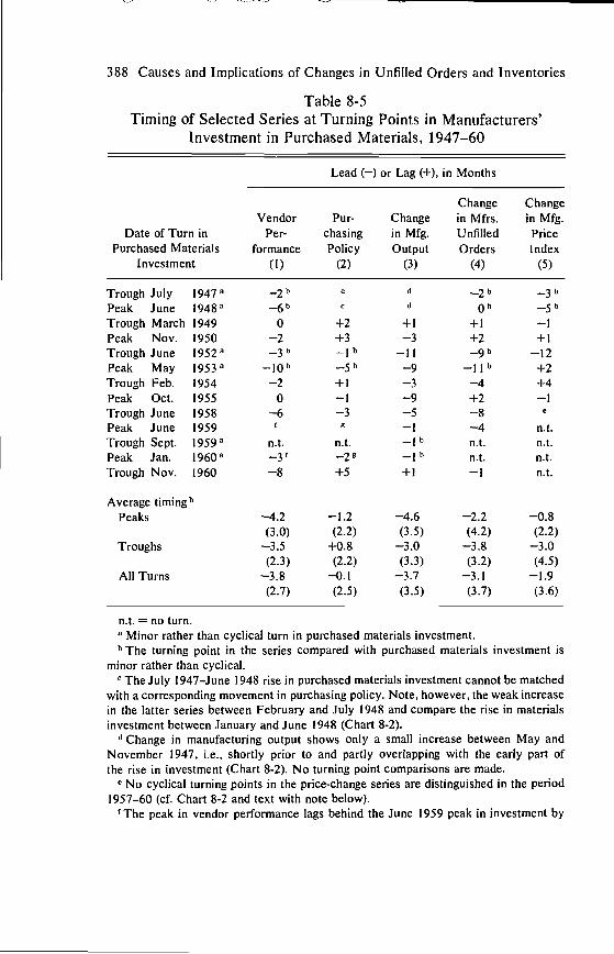
388 Causes and Implications of Changes in Unfilled Orders and Inventories
Table 8-5Timing of Selected Series at Turning Points in Manufacturers'
Investment in Purchased Materials, 1947—60
Lead (—) or Lag (+), in Months
Change ChangeVendor Pur- Change in Mfrs. in Mfg.
Date of Turn in Per- chasing in Mfg. Unfilled PricePurchased Materials formance Policy Output Orders Index
Investment (I) (2) (3) (4) (5)
Trough July 1947 a c d
Peak June b C d 0b
Trough March 1949 0 +2 +1 +1 —1
Peak Nov. 1950 —2 +3 —3 +2 +1
Trough June —12Peak May 1953k' ..9 +2Trough Feb. 1954 —2 +1 —3 —4 +4Peak Oct. 1955 0 —1 —9 +2 —1
Trough June 1958 —6 —3 —5 —8 e
Peak June 1959 f g —1 —4 n.t.
Trough Sept. n.t. n.t. n.t. n.t.
Peak Jan.1960 n.t.
Average timinghPeaks —4.2
(3.0)—1.2
(2.2)—4.6(3.5)
—2.2(4.2)
—0.8(2.2)
Troughs —3.5 +0.8 —3.0 —3.8 —3.0
All Turns(2.3)
—3.8
(2.7)
(2.2)—0.1
(2.5)
(3.3)—3.7
(3.5)
(3.2)—3.1
(3.7)
(4.5)—1.9
(3.6)
n.t. = no turn.a Minor rather than cyclical turn in purchased materials investment.b The turning point in the series compared with purchased materials investment is
minor rather than cyclical.The July 1947—June 1948 rise in purchased materials investment cannot be matched
with a corresponding movement in purchasing policy. Note, however, the weak increasein the latter series between February and July 1948 and compare the rise in materialsinvestment between January and June 1948 (Chart 8-2).
d Change in manufacturing output shows only a small increase between May andNovember 1947, i.e., shortly prior to and partly overlapping with the early part ofthe rise in investment (Chart 8-2). No turning point comparisons are made.
No cyclical turning points in the price-change series are distinguished in the period1957—60 (cf. Chart 8-2 and text with note below).
1The peak in vendor performance lags behind the June 1959 peak in investment by

Orders, Production, and Inventory Investment 389
four months but it would be more appropriate to match it with the secondary January1960 peak in investment, which yields a lead of three months (Chart 8-2).
The peak in purchasing policy lags behind the June 1959 peak in investment by fivemonths, but it would be more appropriate to match it with the secondary January 1960peak in investment, which yields a lead of two months.
Ii Average deviations, in months, are given in parentheses.
from two to five months, with three exceptions, and averaged 3.7months.55
The difference in relative timing between the vendor performanceand the purchasing policy index is interesting because of its consistencywith the presence of what was called earlier the supply conditionseffect; that is, when industrial buyers perceive a lengthening of theaverage delivery periods quoted by their suppliers, they will soon at-tempt to place more long-term orders to protect themselves againstpossible shortages in the future. Conversely, when sellers start quotingshorter delivery periods again, buyers will relax and begin reducingthe average length of their purchasing commitments. Of course, therelation is really a good deal more complicated, for it is definitely oneof mutual dependence and reinforcement rather than unidirectional.An extension of quoted delivery periods may induce more long-termbuying, but it also means in itself an enforced increase of the share ofadvance orders in total purchases.
When more than 50 per cent of suppliers are reported to makeslower deliveries, this is usually a symptom of increased pressures ofdemand upon capacity, and so is an accelerated expansion of unfilledorders. When the pressure subsides, the net percentage of slower de-liveries begins to decline, and a retardation occurs in the backlog ac-cumulation. Investment in purchased-materials inventories is positivelycorrelated with the backlog change (curves 3 and 5), in part becausethe desired volume of these stocks increases with unfilled orders forthe firm's products and in part because of the effects on buyers' be-havior of changes in availability as reflected in the vendor performanceindex. Backlog change leads purchased-materials investment irregu-larly by approximately three months on the average (Table 8-5, column4).
55Altogether, in the 1947—60 period, these comparisons include two lags of 2 months each, two of3 months, and two of 5 months, one of I month, and one of 13 months; and one lead of I month. Theaverages at peaks and troughs are lags of 2.5 and 4.6 months, respectively.
390 Causes and Implications of Changes in Unfilled Orders and Inventories
Investment in purchased materials appears to be more loosely as-sociated with the change in the price index for all manufactures thanwith any of the other series plotted in Chart 8-2. This is consistentwith the results frequently obtained in the regression studies, butmuch doubt remains. It must be reiterated that the wholesale pricedata commonly used in this work probably understate considerablythe cyclical price flexibility. The one period in which investment inmaterials and the change-of-price index moved in markedly similarfashion was the early phase of the Korean War (1950—51 ).56
The relationship that emerges from this analysis is a rather complexone in which fluctuations in materials inventories depend on a numberof factors such as the changes in output, availability of materials, back-logs, and prices. One can identify some periods (e.g., during most of1955) in which purchased-materials investment moved contrary tooutput change and apparently in consonance with changes in orderbacklogs, availability, and prices. At other times, for example, in thelast half of 1959 under the impact of the steel strike (see Chart 8-2),investment in materials and the change in output paralleled each other,while the other series behaved quite differently.
Estimates for Materials Stocks on Hand and on OrderThere are no direct estimates of outstanding purchase orders for
materials, but the new Census data available for the period since 1953provide a usable approximation: the series on unfilled sales ordersheld by manufacturers, classified into the market categories "construc-tion materials and supplies" and "other materials and supplies." Con-sequently, the sum of these two series will be taken to represent the"stock on order" of the purchasers of materials, i.e., their outstandingorders, OUM. The stage-of-fabrication breakdown of total manufac-turers' inventories gives direct estimates of the "stock on hand," i.e.,the inventories of materials and supplies actually held by users, M.Estimates of total "ownership" of materials, OWM, can be obtainedby simple addition of the identically dated, consecutive values of Mand OUM.
Our investment series reflects quantity as well as price changes, of course, and the latter wereexceptionally large at the time. The same circumstance helps to explain the relative weakness inthis period of the association between materials investment and the output change; the use of de-flated figures would make the bulge in investment smaller and more similar to the 1950 contour of theoutput-change series. See Stanback, Postwar Cycles, Chart 6.

Orders, Production, and Inventory Investment 391
Changes in stocks on hand and in stocks on order should occur inresponse to a set of common factors, but the elasticities and the lagsinvolved could well be different for the two components of materialsownership. For example, outstanding orders may be subject toprompter changes and more effective control than materials inventorieson hand. Several questions in this context can be addressed to thenew data, and the following analysis marks a limited effort in thisdirection.
Table 8-6, based on quarterly, seasonally adjusted data, presentsregressions of and on the following independentvariables: current shipments or lagged new orders of all manufacturers(St or used as alternatives); unfilled orders, also for total manu-facturing, as of the end of the preceding quarter, bank rate onshort-term business loans, similarly dated, change from the pre-vious quarter in the price index of intermediate materials and supplies,
and the lagged value of the dependent variable or OUMg_1or OWM1_1).57 Negative coefficients are expected for the interest rate,positive coefficients for the other factors. The signs of the estimatedcoefficients agree with these expectations in each case, except that theimpact of in the inventory regressions is significantly positive.
The positive dependence of on Ng_1 in an equation that also in-cludes and among others, confirms that an increase in thedemand for outputs that require materials results on the average in arise of the desired relative to the actual stock of materials. When isused to replace N1_1, it acquires a similar positive (and highly signifi-cant) coefficient that reflects essentially the same relationship.58 Anadvantage of using is that a predictive lead is gained that is absentin the application of Moreover, in the estimates for outstanding or-ders and for total stocks on hand and on order, it is the equations with
rather than that produce the better statistical results, although
s?The stock variables (M, OUM, OWM, U)and the price variables (PM, i) are last-month valuesin each calendar quarter; the flow variables (S, N) are quarterly averages of monthly data. The in-terest rate, i, is a weighted average for a selected sample of banks in nineteen cities (Federal Re-serve). The price series, PM, covers intermediate materials, supplies, and components purchased bymanufacturers; it is a wholesale price index for one stage of processing, 1957—59 = 100 (U.S. De-partment of Labor, Bureau of Labor Statistics). The other data are taken from U.S. Department ofCommerce, Bureau of the Census, Ma,u.ifacturers' Ship,nenis, Inventories, and Orders: I 947—1963(Revised), Washington, D.C., 1963, and the recent issues of the Survey of Business; all arein millions of dollars.
—" and N1_1 are, of course, highly correlated (r = .992). The regression with S1 yields a higher
R2 than that with but the difference is quite small (Table 8-6, columns I and 2).

392 Causes and Implications of Changes in Unfilled Orders and Inventories
Table 8-6Regressions for Inventories, Outstanding Orders, and TotalInventories on Hand and on Order of Materials Purchased
from Manufacturers, Quarterly, 1954—66
Con-stantTerm
Regression Coefficients LaggedDependent
St Ne_i Variable a R2
(1) (2) (3) (4) (5) (6) (7) (8)
ESTIMATES FOR INVENTORIES (Me) b
1,746.5 .109 .026 5.566 2.561 .532 .982(600.1) (.019) (.007) (1.694) (0.910) (.088)
1,785.3 .097 .022 5.103 2.417 .574 .980(673.5) (.020) (.007) (1.785) (0.988) (.092)
ESTIMATES FOR OUTSTANDING ORDERS
1,304.9 .182 .271 —14.461 7.600 .382 .940(1,816.2) (.055) (.141) (5.008) (3.800) (.272)2,218.5 .204 .251 —16.524 6.354 .405 .945(1,809.2) (.052) (.135) (4.856) (3.708) (.258)
ESTIMATES FOR INVENTORIES ON HAND AND ON ORDER
3,992.0 .322 .347 —5.428 9.914 .307 .964(1,651.7) (.054) (.134) (6.470) - (3.697) (.235)5,326.1 .341 .366 —6.337 8.420 .251 .967
(1,626.6) (.051) (.126) (6.107) (3.533) (.223)
Note: Standard errors of the coefficients are given underneath in parentheses. S, N,and U denote, respectively, the current-dollar values of shipments, new orders, and un-filled orders, for total manufacturing; i is the bank rate of interest on business loansin nineteen cities; is the change in the wholesale price index for intermediatematerials, supplies, etc. = x 100; see text and note 70).
a for the equations in the first two lines; OUM,_1 for third and fourth lines; andfor last two lines. See notes b, c, and d, following.
b The dependent variable = purchased-materials inventories, total manufacturing.CThe dependent variable = unfilled orders of the market category "materials,
supplies, and intermediate products" (see text).ci The dependent variable OWMC = M1 + OUM,.
again the differences are marginal. Outstanding orders for materialsappear to be generally more sensitive than the inventories to changesin demand, which is consistent with the notion that firms can adjustOUM considerably better than M.59
The short-run elasticities at the point of the means with respect to 5,, N,_,, and U,_,, respec-tively, are; for M,, 0.177, 0.157, and 0.072 or 0.060; for OUM,, 0.240, 0.266, and 0.600 or 0.555;
Orders, Production, and Inventory Investment 393
Unfilled orders of manufacturers at the end of the preceding quarterhave in each case a significant positive effect on the current inventoriesand/or outstanding orders of materials (column 4). It should be noted,however, that the partial correlations for are not high and aresmaller throughout than those for either St or N1_1.6°
The net impact of changes in the bank rate on business loans onmaterials stocks on hand is quite significant but positive, according toboth the first and the second equation in Table 8-6. However, strongernegative effects are obtained for in the regressions for outstandingorders (particularly in the estimates with N1_1).61 Since negative co-efficients are expected, this finding, if valid, would again suggest thatadjustments are made more promptly and with greater success in out-standing orders than in the physical stock of materials. For the aggre-gate of stocks on hand and on order, the results are mixed: The co-efficients of are negative but very low relative to their standarderrors.
If price expectations have large extrapolative components, so thatrises in the level of materials prices are associated with forecasts offurther rises, at least some of the firms would probably attempt to hedgeagainst or beat the price hike by accelerating their purchases in pe-riods of inflationary developments. The evidence on the presence ofsuch "speculative" behavior is mixed, as reported before (see textand Tables 8-2 and 8-3). Our estimates in Table 8-6, column 6, showfairly significant coefficients of the price-change variable withthe expected positive signs. Since the measured price index changesare very small, their coefficients in absolute value are large, and itseemed advisable to apply a scale factor to this variable.62 It is pos-
for OWMV, 0.234, 0.246, and 0.425 or 0.448. (The first of the estimates for U,_1 refers to the equa-tions with the second to those with The elasticity of OUMC to is relatively high, butthis must be discounted because total backlogs represent a massive aggregate that includes outstand-ing orders for materials. (The simple correlation between OUM, and U,_1 is 0.953. The averagevalue of U in the regression period was $55.3 billion; of OUM, $24.7 billion.)
60The highest of these partials with U,_1 are .499, .281, and .404 forM,, OUM,, and OWM,, re-spectively, whereas the corresponding partials with S, are .659, .450, and .672, and those with N,_1are .604, .514, and .716.
°' The partial correlations of with M, and OUM, are .400 and —.461, respectively (this is forthe equations with N,—1; the estimates for the equations with St are .448 and—.403). The correspond-ing elasticity figures are .122 and —.318 (or .133 and —.278).
62 That is, the estimates in Table 8-6 refer to APM? = 100 x Had the observed changesbeen used without this adjustment, the coefficients in column 6 would have been 100 times larger,ranging from 241.74 to 991.36. A casual glance at such large values could be misleading— suggestiveof stronger effects than are actually involved. The partial correlations, for example, are rather low,varying from .253 to .394.
394 Causes and Implications of Changes in Unfilled Orders and Inventories
sible that this factor operates with longer and more complex lags, butthe evidence on this point is fragmentary and at best only suggestive.63
In the first equation of Table 8-6, subtracting the coefficient offrom 1.000 gives 0.468, which, when interpreted in accordance withthe flexible-accelerator model, means that a little less than one-half ofthe discrepancy between the available and desired stock of materialswould on the average be targeted for correction within one quarter ofa year. The corresponding fraction is somewhat lower (0.426) for thesecond equation, which includes instead of Some other inven-tory studies estimate the adjustments to be much slower than that, butthe sluggishness thus implied seems to me rather implausible.64
One would expect the adjustments to be speedier for outstandingorders than for stocks on hand, and the estimates in column 7 of Table8-6 are consistent with this hypothesis in that the coefficients of 0 UM1_1are lower than those of The regression results suggest that about0.6, or a slightly higher fraction, of the gap between the actual and theplanned level of outstanding orders would on the average over time becorrected in any one quarter. (However, unlike the coefficients ofin the estimates for inventories, the coefficients of have rel-atively large standard errors; they are significantly different from zeroat the 10 per cent but not at the 5 per cent level, according to one-sidedt tests. In the equations for total stocks on hand and on order, the co-efficients of are still lower absolutely and relative to theirstandard errors.)
Chart 8-3 compares the actual values of inventories, outstanding or-ders, and stocks on hand and on order of materials and supplies withthe corresponding estimates based on the equations from Table 8-6,lines 2, 4, and 6 (these are the regressions that include the new ordersvariable It is clear that the fits, which are somewhat better forM and OWM than for OUM, are generally close. Relatively large re-siduals and differing patterns in actuals and estimates are observed in1959. However, the major steel strike then in progress created un-usually severe disturbances. Even so, the calculated values tend to lagbehind by a quarter at the turns in the recorded values and to under-
°3The effects of approximate those of in the equations for outstanding orders, butthey are considerably weaker and of low or doubtful significance in the equations for stocks on hand.
°4The result here is similar to that obtained by Lovell in his all-manufacturing regression for ma-terials and goods in process (see Table 8-3, first line).
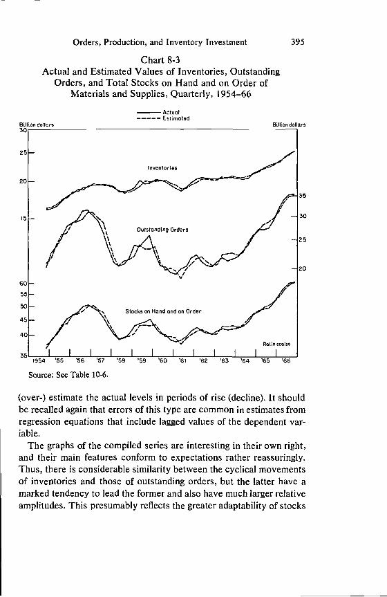
Orders, Production, and Inventory Investment 395
Chart 8-3Actual and Estimated Values of Inventories, Outstanding
Orders, and Total Stocks on I-land and on Order ofMaterials and Supplies, Quarterly, 1954—66
(over-) estimate the actual levels in periods of rise (decline). It shouldbe recalled again that errors of this type are common in estimates fromregression equations that include lagged values of the dependent var-iable.
The graphs of the compiled series are interesting in their own right,and their main features conform to expectations rather reassuringly.Thus, there is considerable similarity between the cyclical movementsof inventories and those of outstanding orders, but the latter have amarked tendency to lead the former and also have much larger relativeamplitudes. This presumably reflects the greater adaptability of stocks
ActucilEstimated
Source: See Table 10-6.
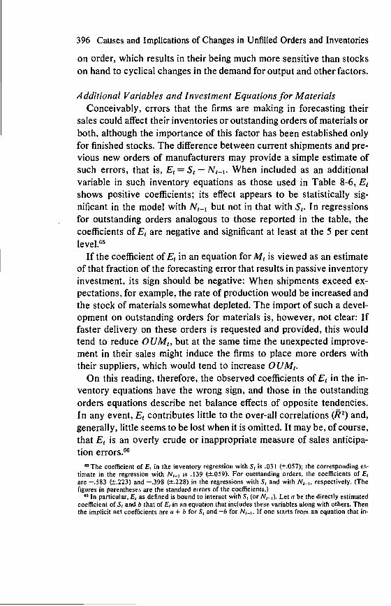
396 Causes and Implications of Changes in Unfilled Orders and Inventories
on order, which results in their being much more sensitive than stockson hand to cyclical changes in the demand for output and other factors.
Additional Variables and investment Equations for MaterialsConceivably, errors that the firms are making in forecasting their
sales could affect their inventories or outstanding orders of materials orboth, although the importance of this factor has been established onlyfor finished stocks. The difference between current shipments and pre-vious new orders of manufacturers may provide a simple estimate ofsuch errors, that is, E1 = — When included as an additionalvariable in such inventory equations as those used in Table 8-6,shows positive coefficients; its effect appears to be statistically sig-nificant in the model with but not in that with In regressionsfor outstanding orders analogous to those reported in the table, thecoefficients of are negative and significant at least at the 5 per centlevel.65
If the coefficient of in an equation for is viewed as an estimateof that fraction of the forecasting error that results in passive inventoryinvestment, its sign should be negative: When shipments exceed ex-pectations, for example, the rate of production would be increased andthe stock of materials somewhat depleted. The import of such a devel-opment on outstanding orders for materials is, however, not clear: Iffaster delivery on these orders is requested and provided, this wouldtend to reduce but at the same time the unexpected improve-ment in their sales might induce the firms to place more orders withtheir suppliers, which would tend to increase
On this reading, therefore, the observed coefficients of in the in-ventory equations have the wrong sign, and those in the outstandingorders equations describe net balance effects of opposite tendencies.In any event, contributes little to the over-all correlations (R2) and,generally, little seems to be lost when it is omitted. It may be, of course,that is an overly crude or inappropriate measure of sales anticipa-tion errors.6°
The coefficient of E1 in the inventory regression with S, is .031 (±.057); the corresponding es-timate in the regression with N1...1 is .139 (±.059). For outstanding orders, the coefficients of E1are —.583 (±.223) and —.398 (±.228) in the regressions with S1 and with N1_1, respectively. (Thefigures in parentheses are the standard errors of the coefficients.)
In particular, E1 as defined is bound to interact with (or N1_1). Let a be the directly estimatedcoefficient of S1 and b that of E1 in an equation that includes these variables along with others. Thenthe implicit net coefficients are a + b for S1 and—b for N1_1. If one starts from an equation that in-

Orders, Production, and Inventory Investment 397
Significant changes in the prevailing delivery periods for materialsand supplies are certainly likely to influence outstanding orders forthese goods. For example, the immediate impact of an over-all length-ening of these lags should be to reduce the rate of deliveries, whichtends to increase the amount of orders outstanding. This effect maylater be reinforced if users place more orders for materials to protectthemselves against possible shortages. The influence of changes in theaverage delivery period for materials on inventories M is more indirectand should be weaker; moreover, here reactions in the opposite direc-tion can be more readily envisaged.67
The average delivery lag for materials may be approximated by theratio of unfilled orders to shipments for the industries that producematerials, that is, = A quarterly series of such ra-tios can be computed from the new Census market-category data.68When is included along with the other variables from Table 8-6in the inventory equations, it has in each case a negative coefficient,which, however, is definitely not significant, since the coefficient issmaller than its standard error. Since no strong effect of this factor onM had been expected, this result is not implausible. When is
similarly added to the equations for outstanding orders, the results arenot meaningful; indeed, the relationships estimated in Table 8-6 for0 are then thoroughly disrupted (the coefficients of St and N1....1 be-come negative!). This is apparently because of the interaction ofwith the lagged value of the dependent variable, 0 and the back-log of unfilled orders of manufacturers, When these two factorsare omitted, enters the regression with a highly significant pos-itive coefficient, and the remaining variables also have relatively largecoefficients with the expected signs. When either or 0 is
etudes and E,, their measured effects will be a and a + b, respectively, which implies the samenet coefficients as before for S1 and N1_1. The coefficient of (or N1_1) in the regression for inven-tories that includes E, is .108 (±.019); the corresponding estimate in the regression for outstandingorders is .185 (±.052). These figures are extremely close to the coefficients for S1 in the first and thirdlines of Table 8-6. The coefficients of the other variables are only very slightly affected by the in-clusion of
67 The same demand pressures that generate an increase in the delivery lags may also cause therates of utilization of materials to rise. The latter factor would work to reduce the stocks of mate-nals on hand.
68 series combines data for two categories, as identified early in the previous section. The un-filled (= outstanding) orders, OUM, are as of the last month of the quarter (1— 1) when the ship-ments (deliveries) of materials, DM, refer to the tth quarter. Most of the time, the delivery periodsfor materials and supplies are relatively short; they average 1.607 months, with a standard deviationof 0.297.
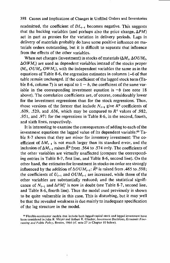
398 Causes and Implications of Changes in Unfilled Orders and Inventories
readmitted, the coefficient of becomes negative. This suggeststhat the backlog variables (and perhaps also the price change,act in part as proxies for the variation in delivery periods. Lags indelivery of materials probably do have some positive influence on ma-terials orders outstanding, but it is difficult to separate that influencefrom the effects of the other variables.
When net changes (investment) in stocks of materialsare used as dependent variables instead of the stocks proper
(Me, with the independent variables the same as in theequations of Table 8-6, the regression estimates in columns 1—6 of thattable remain unchanged. If the coefficient of the lagged stock term (Ta-ble 8-6, column 7) is set equal to 1 — b, the coefficient of the same var-iable in the corresponding investment equation is —b (see note 18above). The correlation coefficients are, of course, considerably lowerfor the investment regressions than for the stock regressions. Thus,those versions of the former that include give R2 coefficients of.609, .520, and .636, which may be compared to R2 values of .982,.95 1, and .971 for the regressions in Table 8-6, in the second, fourth,and sixth lines, respectively.
It is interesting to examine the consequences of adding to each of theinvestment equations the lagged value of its dependent variable.69 Ta-ble 8-7 shows that they are minor for inventory investment: The co-efficient of is not much larger than its standard error, and theinclusion of raises from .564 to .574 only. The coefficients ofthe other variables are virtually unaffected (compare the correspond-ing entries in Table 8-7, first line, and Table 8-6, second line). On theother hand, the estimates for investment in stocks on order are stronglyinfluenced by the addition R2 is raised from .465 to .598;the coefficients of U1_1 and are increased, while those of theother variables are substantially reduced; and the statistical signifi-cance of and is now in doubt (see Table 8-7, second line,and Table 8-6, fourth line). Thus the model used previously is shownto be quite vulnerable in this case. This is disturbing, but it may wellbe that the revealed weakness is due mainly to inadequate specificationof the lag structure in the model.
69 Flexible-accelerator models that include both lagged capital stock and lagged investment havebeen considered in John R. Meyer and Robert R. Glauber, Investment Decisions, Economic Fore-casting and Public Policy, Boston, 1964 (cf. note 27 in Chapter 10 below).

Orders, Production, and Inventory Investment 399
Table 8-7Regressions for Investment in Materials Inventories, Outstanding
Orders, and Inventories on Hand and on Order,Quarterly, 1954—66
Dc-pendent
Van-able
Con-stantTerm
(1)
Regression Coefficients
(2) (3) (4)APMI°
(5)
LaggedStockLevel a
(6)
LaggedDe-
pendentVan-able b
(7) (8)
1,964.1
(677.2)
1,094.7
(1,594.5)
5,845.3(1,407.7)
.093
(.020)
.077
(.056)
.242(.050)
.019
(.007)
.428
(.126)
.365(.109)
5.377
(1.774)
—8.552
(4.679)
1.878(5.510)
2.412(0.976)3.679
(3.286)
5.193(3.150)
—.430
(.091)—.937
(.240)
—.760(.192)
.158(.1 11)
.520
(.133)
.450(.113)
.574
.598
.698
Note: Standard errors of the coefficients are given underneath in parentheses. For anexplanation of the symbols, see the note to Table 8-6.
a for the equation in the first line; for the second line; and forthe last line.
for the equation in the first line; for the second line; andfor the last line. See Table 8-6, notes a, b, and c. Quarter-to-quarter change is denoted
The results for investment in total materials stocks on hand and onorder are more satisfactory. The over-all correlation is here fairly highfor an equation with first differences (R2 = .736), and all but two of theregression coefficients are more than three times larger than their stand-ard errors. However, is considerably less effective here than inthe equation without and the coeffcient of becomes pos-itive and is reduced to a fraction of its standard error (compare Tables8-7 and 8-6).
Estimates in Real TermsAt least some of the aspects of inventory behavior require in prin-
ciple an analysis in terms of physical quantities or price-deflated values,a notable example being the possible price-change effects on inventorypolicies. An attempt was therefore made to discover what may be cx-

400 Causes and Implications of Changes in Unfilled Orders and Inventories
pected in the present context from the use of series expressed in con-stant dollars. The very limited scope and purpose of this effort must beemphasized, along with the need to recognize that deflation of aggre-gative data on stocks and orders presents particularly difficult estima-tion problems and may result in large measurement errors.
The price index PM for materials has been used as a deflator for thedependent variables, to produce the series in constant (1957—59 = 100)dollars, M*, OUM*, and OWM*. The all-manufacturing series havebeen deflated by means of the wholesale price index for manufacturedproducts 70
The models underlying Table 8-6 were then re-estimated with theconstant-dollar series replacing the current-dollar ones. Table 8-8,lines 1—3, shows the results for the equations that include Ne...., (cf. withTable 8-6). The coefficients of and the lagged values of thedependent variables are very close indeed to the coefficients of
etc., in Table 8-6. The coefficients of are also similar in thetwo sets of regressions. However, the significance of the coefficients
is considerably reduced in the estimates with price-deflateddata, suggesting that some (but by no means all) of the previously ob-served effects of this variable must be attributed to the purely nominalmovements of the value aggregates for stocks on hand and/or on order.The values of R2 in the two tables differ very little.
Rising prices may offset some of the increase in the cost of borrow-ing (and gains from lending) that result from rising interest rates. Tothe extent that inflationary expectations existed in the period surveyed,the deterrent effect of increasing interest costs was presumably blunted.It seemed advisable, therefore, to examine the effectiveness in the con-stant-dollar equations of the real interest rate j*; but since this variableinvolves the expected changes in the general price level, it is not di-rectly observable. The measure of I adopted here is the nominal rateminus the last actual change in prices, both expressed in percentagesper year, but this proxy may be a poor one.7'
As shown in the last three lines of Table 8-8, the coefficients of i7,are all negative, but the one in the inventory regression is not signifi-cantly different from zero. The coefficient of in the same regres-
Asterisks denote the deflated series. That is, = 100 (M,f PM1), = 100 (N1/P1), etc. (wherePM is the price index for materials and P the index for all manufactured products).
71 The price series used in this computation of is the all-manufacturing price index P. While notas comprehensive as might be desired, this index was deemed representative enough for our purpose.
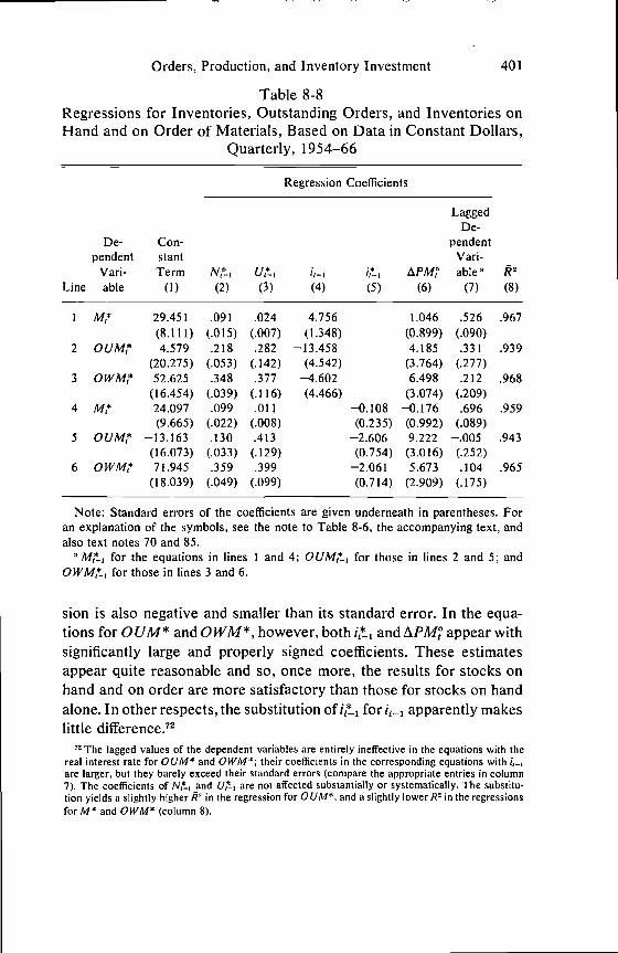
fl
Orders, Production, and Inventory Investment 401
Table 8-8Regressions for Inventories, Outstanding Orders, and Inventories onHand and on Order of Materials, Based on Data in Constant Dollars,
Quarterly, 1954—66
Line
De-pendent
Van-able
Con-stantTerm
(1)
Regression Coefficients
(2) (3) (4) (5) (6)
LaggedDe-
pendentVan-able a
(7)if2(8)
1
2
3
4
5
6
OUMI*
OWM7
OUM1*
OWM1*
29.451(8.111)4.579
(20.275)52.625
(16.454)24.097(9.665)
—13.163(16.073)71.945
(18.039)
.091
(.015).218
(.053).348
(.039).099
(.022).130(.033).359
(.049)
.024(.007).282
(.142).377
(.116).011
(.008).413(.129).399
(.099)
4.756(1.348)
—13.458(4.542)
—4.602(4.466)
—0.108(0.235)
—2.606(0.754)
—2.061(0.714)
1.046(0.899)4.185
(3.764)6.498(3.074)
—0.176(0.992)9.222(3.016)5.673(2.909)
.526(.090).331
(.277).212(.209).696
(.089)—.005(.252).104
(.175)
.967
.939
.968
.959
.943
.965
Note: Standard errors of the coefficients are given underneath in parentheses. Foran explanation of the symbols, see the note to Table 8-6, the accompanying text, andalso text notes 70 and 85.
a for the equations in lines I and 4; for those in lines 2 and 5; andOWM1t.1 for those in lines 3 and 6.
sion is also negative and smaller than its standard error. In the equa-tions for OUM* and OWM*, however, both and appear withsignificantly large and properly signed coefficients. These estimatesappear quite reasonable and so, once more, the results for stocks onhand and on order are more satisfactory than those for stocks on handalone. In other respects, the substitution of for apparently makeslittle difference.72
72 The lagged values of the dependent variables are entirely ineffective in the equations with thereal interest rate for OUM* and OWM*; their coefficients in the corresponding equations with if_Iare larger, but they barely exceed their standard errors (compare the appropriate entries in column7). The coefficients of and U,*_1 are not affected substantially or systematically. The substitu-tion yields a slightly higher R2 in the regression for OUM*, and a slightly lowerR2 in the regressionsfor M* and OWM* (column 8).
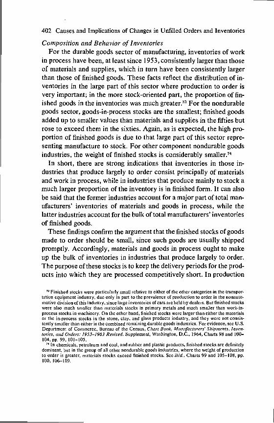
402 Causes and Implications of Changes in Unfilled Orders and Inventories
Composition and Behavior of InventoriesFor the durable goods sector of manufacturing, inventories of work
in process have been, at least since 1953, consistently larger than thoseof materials and supplies, which in turn have been consistently largerthan those of finished goods. These facts reflect the distribution of in-ventories in the large part of this sector where production to order isvery important; in the more stock-oriented part, the proportion of fin-ished goods in the inventories was much greater.73 For the nondurablegoods sector, goods-in-process stocks are the smallest; finished goodsadded up to smaller values than materials and supplies in the fifties butrose to exceed them in the sixties. Again, as is expected, the high pro-portion of finished goods is due to that large part of this sector repre-senting manufacture to stock. For other component nondurable goodsindustries, the weight of finished stocks is considerably smaller.74
In short, there are strong indications that inventories in those in-dustries that produce largely to order consist principally of materialsand work in process, while in industries that produce mainly to stock amuch larger proportion of the inventory is in finished form. It can alsobe said that the former industries account for a major part of total man-ufacturers' inventories of materials and goods in process, while thelatter industries account for the bulk of total manufacturers' inventoriesof finished goods.
These findings confirm the argument that the finished stocks of goodsmade to order should be small, since such goods are usually shippedpromptly. Accordingly, materials and goods in process ought to makeup the bulk of inventories in industries that produce largely to order.The purpose of these stocks is to keep the delivery periods for the prod-ucts into which they are processed competitively short. In production
Finished stocks were particularly small relative to either of the other categories in the transpor-tation equipment industry, due only in part to the prevalence of production to order in the nonauto-motive division of this industry, since large inventories of cars are held by dealers. But finished stockswere also much smaller than materials stocks in primary metals and much smaller than work-in-process stocks in machinery. On the other hand, finished stocks were larger than either the materialsor the in-process stocks in the stone, clay, and glass products industry, and they were not consis-tently smaller than either in the combined remaining durable goods industries. For evidence, see U.S.Department of Commerce, Bureau of the Census, Chart Book, Manufacturers' Shipments, Inven-tories, Orders: 1953—1963 Revised, Supplement, Washington, D.C., 1964, Charts 98 and 100—104, pp. 99, 101—105.
In chemicals, petroleum and coal, and rubber and plastic products, finished stocks are definitelydominant, but in the group of all other nondurable goods industries, where the weight of productionto order is greater, materials stocks exceed finished stocks. See ibid., Charts 99 and 105—108, pp.100, 106—109.
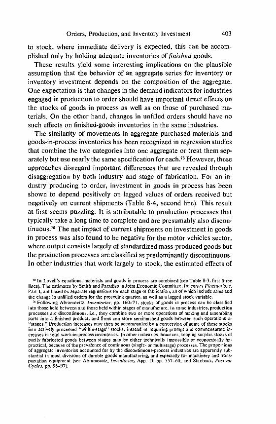
Orders, Production, and Inventory Investment 403
to stock, where immediate delivery is expected, this can be accom-plished only by holding adequate inventories of finished goods.
These results yield some interesting implications on the plausibleassumption that the behavior of an aggregate series for inventory orinventory investment depends on the composition of the aggregate.One expectation is that changes in the demand indicators for industriesengaged in production to order should have important direct effects onthe stocks of goods in process as well as on those of purchased ma-terials. On the other hand, changes in unfilled orders should have nosuch effects on finished-goods inventories in the same industries.
The similarity of movements in aggregate purchased-materials andgoods-in-process inventories has been recognized in regression studiesthat combine the two categories into one aggregate or treat them sep-arately but use nearly the same specification for each.75 However, theseapproaches disregard important differences that are revealed throughdisaggregation by both industry and stage of fabrication. For an in-dustry producing to order, investment in goods in process has beenshown to depend positively on lagged values of orders received butnegatively on current shipments (Table 8-4, second line). This resultat first seems puzzling. It is attributable to production processes thattypically take a long time to complete and are presumably also discon-tinuous.76 The net impact of current shipments on investment in goodsin process was also found to be negative for the motor vehicles sector,where output consists largely of standardized mass-produced goods butthe production processes are classified as predominantly discontinuous.In other industries that work largely to stock, the estimated effects of
"In Lovell's equations, materials and goods in process are combined (see Table 8-3, first threelines). The estimates by Smith and Paradiso in Joint Economic Committee, Inventory Fluctuations,Part 1, are based on separate regressions for each stage of fabrication, all of which include sales andthe change in unfilled orders for the preceding quarter, as welt as a lagged stock variable.
Following Abramovitz, inventories, pp. 160—71, stocks of goods in process can be classifiedinto those held between and those held within stages of manufacture. In some industries, productionprocesses are discontinuous, i.e., they combine two or more operations of making and assemblingparts into a finished product, and firms can store semifinished goods between such operations or"stages." Production increases may then be accompanied by a conversion of some of these stocksinto actively processed "within-stage" stocks, instead of requiring prompt and commensurate in-creases in total work.in-process inventories. In other industries, however, keeping surplus stocks ofpartly fabricated goods between stages may be either technically impossible or economically im-practical, because of the prevalence of continuous (single- or multistage) processes. The proportionsof aggregate inventories accounted for by the discontinuous-process industries are apparently sub-stantial in most divisions of durable goods manufacturing, and especially for machinery and trans-portation equipment (see Abramovitz, Inventories, App. D, pp. 557—60, and Stanback, PostwarCycles, pp. 96—97).
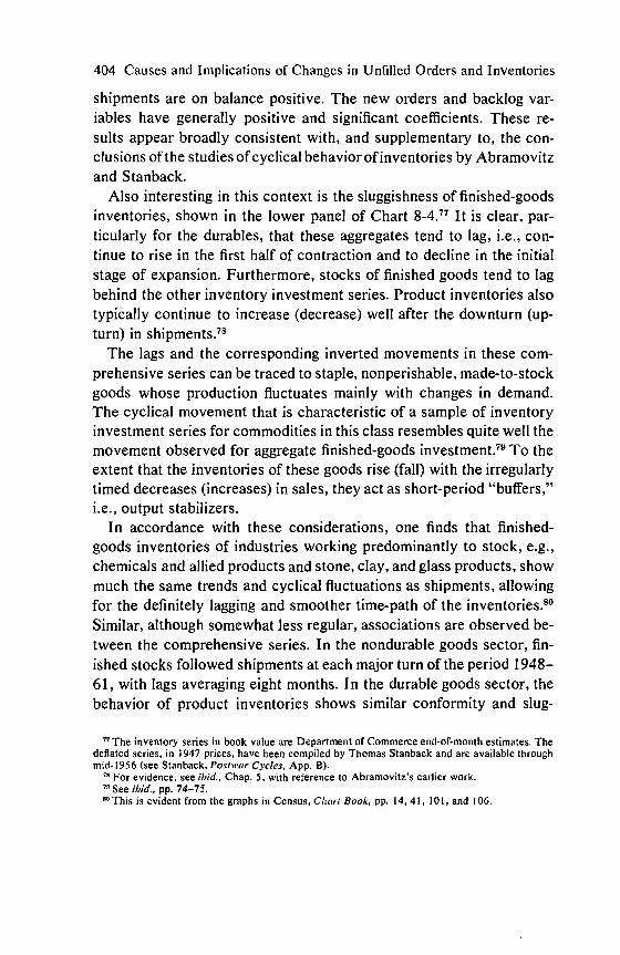
404 Causes and Implications of Changes in Unfilled Orders and Inventories
shipments are on balance positive. The new orders and backlog var-iables have generally positive and significant coefficients. These re-suits appear broadly consistent with, and supplementary to, the con-clusions of the studies of cyclical behavior of inventories by Abramovitzand Stanback.
Also interesting in this context is the sluggishness of finished-goodsinventories, shown in the lower panel of Chart It is clear, par-ticularly for the durables, that these aggregates tend to lag, i.e., con-tinue to rise in the first half of contraction and to decline in the initialstage of expansion. Furthermore, stocks of finished goods tend to lagbehind the other inventory investment series. Product inventories alsotypically continue to increase (decrease) well after the downturn (up-turn) in shipments.78
The lags and the corresponding inverted movements in these com-prehensive series can be traced to staple, nonperishable, made-to-stockgoods whose production fluctuates mainly with changes in demand.The cyclical movement that is characteristic of a sample of inventoryinvestment series for commodities in this class resembles quite well themovement observed for aggregate finished-goods investment.79 To theextent that the inventories of these goods rise (fall) with the irregularlytimed decreases (increases) in sales, they act as short-period "buffers,"i.e., output stabilizers.
In accordance with these considerations, one finds that finished-goods inventories of industries working predominantly to stock, e.g.,chemicals and allied products and stone, clay, and glass products, showmuch the same trends and cyclical fluctuations as shipments, allowingfor the definitely lagging and smoother time-path of the inventories.80Similar, although somewhat less regular, associations are observed be-tween the comprehensive series. In the nondurable goods sector, fin-ished stocks followed shipments at each major turn of the period 1948—61, with lags averaging eight months. In the durable goods sector, thebehavior of product inventories shows similar conformity and slug-
The inventory series in book value are Department of Commerce end-of-month estimates. Thedeflated series, in 1947 prices, have been compiled by Thomas Stanback and are available throughmid-1956 (see Stanback, Postwar Cycles, App. B).
78 For evidence, see ibid., Chap. 5, with reference to Abramovitz's earlier work.See ibid., pp. 74—75.
80This is evident from the graphs in Census, Chart Book, pp. 14, 41, 101, and 106.

Orders, Production, and Inventory Investment 405
Chart 8-4Unfilled Order Backlogs and Finished-Goods Inventories in
Current and Constant Prices, Durable and NondurableGoods Industries, 1948—6 1
Note: Shaded areas represent business cycle contractions; unshaded areas, expan-sions. Triangles identify peaks and troughs in the deflated series; dots, undeflated series;circles, retardations.
Source: See note 76, in this chapter.
Unfilled Order Backlogs
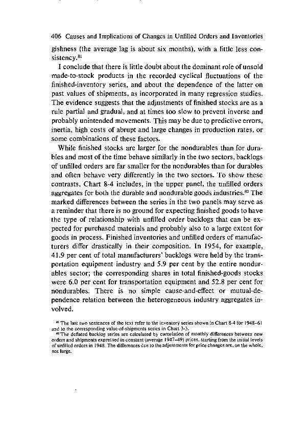
406 Causes and Implications of Changes in Unfilled Orders and Inventories
gishness (the average lag is about six months), with a little less con-sistency.8'
I conclude that there is little doubt about the dominant role of unsoldmade-to-stock products in the recorded cyclical fluctuations of thefinished-inventory series, and about the dependence of the latter onpast values of shipments, as incorporated in many regression studies.The evidence suggests that the adjustments of finished stocks are as arule partial and gradual, and at times too slow to prevent inverse andprobably unintended movements. This may be due to predictive errors,inertia, high costs of abrupt and large changes in production rates, orsome combinations of these factors.
While finished stocks are larger for the nondurables than for dura-bles and most of the time behave similarly in the two sectors, backlogsof unfilled orders are far smaller for the nondurables than for durablesand often behave very differently in the two sectors. To show thesecontrasts, Chart 8-4 includes, in the upper panel, the unfilled ordersaggregates for both the durable and nondurable goods industries.82 Themarked differences between the series in the two panels may serve asa reminder that there is no ground for expecting finished goods to havethe type of relationship with unfilled order backlogs that can be ex-pected for purchased materials and probably also to a large extent forgoods in process. Finished inventories and unfilled orders of manufac-turers differ drastically in their composition. In 1954, for example,41.9 per cent of total manufacturers' backlogs were held by the trans-portation equipment industry and 5.9 per cent by the entire nondur-ables sector; the corresponding shares in total finished-goods stockswere 6.0 per cent for transportation equipment and 52.8 per cent fornondurables. There is no simple cause-and-effect or mutual-de-pendence relation between the heterogeneous industry aggregates in-volved.
81 The last two sentences of the text refer to the inventory series shown in Chart 8-4 for 1948—61and to the corresponding value-of-shipments series in Chart 3-3.
82 The deflated backlog series are calculated by cumulation of monthly differences between neworders and shipments expressed in constant (average 1947—49) prices, starting from the initial levelsof unfilled orders in 1948. The differences due to the adjustments for price changes are, on the whole,not large.
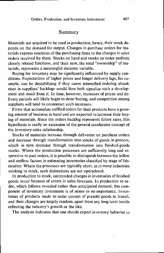
Orders, Production, and Inventory Investment 407
Summary
Materials are acquired to be used in production; hence, their stock de-pends on the demand for output. Changes in purchase orders for ma-terials express reactions of the purchasing firms to the changes in salesorders received by them. Stocks on hand and stocks on order performclosely related functions, and their sum, the total "ownership" of ma-terials, represents a meaningful decision variable.
Buying for inventory may be significantly influenced by supply con-ditions. Expectations of higher prices and longer delivery lags, for ex-ample, can be destabilizing if they cause intensified ordering ahead;rises in suppliers' backlogs would then both signalize such a develop-ment and result from it. In time, however, increases of prices and de-livery periods will likely begin to deter buying, and competition amongsuppliers will tend to counteract such increases.
Firms that accumulate unfilled orders for their products have a grow-ing amount of business in hand and are expected to increase their buy-ing of materials. Since the orders backlog represents future sales, thishypothesis is really an extension of the general accelerator concept ofthe inventory-sales relationship.
Stocks of materials increase through deliveries on purchase ordersand decrease through transformation into stocks of goods in process,which in turn decrease through transformation into finished-goodsstocks. Where the production processes are sufficiently long and re-sponsive to past orders, it is possible to distinguish between the inflowand outflow factors in estimating inventories classified by stage of fab-rication. Where the processes are typically short, as in many industriesworking to stock, such distinctions are not operational.
In production to stock, unintended changes in inventories of finishedgoods occur because of errors in sales forecasts. In production to or-der, which follows revealed rather than anticipated demand, this com-ponent of inventory investment is of minor or no importance. Inven-tories of products made to order consist of presold goods in transit,and their changes are largely random, apart from any long-term trendsreflecting the industry's growth or the like.
The analysis indicates that one should expect inventory behavior to

408 Causes and Implications of Changes in Unfilled Orders and Inventories
show systematic differences both between stages of fabrication andbetween industries producing mainly to stock and industries producingmainly to order. A review of literature brings out evidence that is gen-erally consistent with this position but is rather severely limited by (1)frequent neglect of the required distinctions and (2) inadequacy of thedata.
Census series for the period since 1953 permit the construction ofestimates of outstanding purchase orders for materials (OUM). Quar-terly regressions show OUM to be positively associated with the pre-vious values of new and unfilled orders of all manufacturers and withthe change in the price index for materials, and negatively associatedwith the lagged interest rate on short-term bank loans to business.These signs of the estimated coefficients agree with expectations. Pur-chased-material inventories (M) are less sensitive than 0 UM to changesin demand (the lagged order variables). The results are consistent withthe view that firms can and do adjust their orders for materials con-siderably better than their inventories of materials. Typically, OUMare larger than M and have cyclical fluctuations of greater amplitudeand earlier timing. The adjustments of M and, particularly, 0 UM to-ward desired levels do not involve very long lags. (Some recent studiesof inventory behavior produced estimates that imply rather implausiblysluggish adjustments.)
Postwar data are in accord with expectations in indicating that in-ventories in those industries that produce largely to order consist prin-cipally of materials and goods in process, while inventories in indus-tries that produce mainly to stock are held in much larger proportionsin finished form. Stocks of finished goods tend to lag behind materialsand work in process, and also behind shipments. These lags are attrib-utable to nonperishable made-to-stock goods, which constitute the larg-est component category of finished stocks.