OptiSystem User Book - dru5cjyjifvrg.cloudfront.net · and fiber optic amplifiers. OptiSystem...

OptiSystemGetting Started

Optical Communication System Design Software

Version 7.0 for Windows® XP/Vista

OptiSystemGetting StartedOptical Communication System Design Software

Copyright © 2008 OptiwaveAll rights reserved.

All OptiSystem documents, including this one, and the information contained therein, is copyright material.

No part of this document may be reproduced, stored in a retrieval system, or transmitted in any form or by any means whatsoever, including recording, photocopying, or faxing, without prior written approval of Optiwave.

DisclaimerOptiwave makes no representation or warranty with respect to the adequacy of this documentation or the programs which it describes for any particular purpose or with respect to its adequacy to produce any particular result. In no event shall Optiwave, its employees, its contractors or the authors of this documentation be liable for special, direct, indirect or consequential damages, losses, costs, charges, claims, demands, or claim for lost profits, fees or expenses of any nature or kind.

Technical support

If you purchased Optiwave software from a distributor that is not listed here, please send technical questions to your distributor.

Optiwave Canada/USTel (613) 224-4700 E-mail [email protected]

Fax (613) 224-4706 URL www.optiwave.com

Cybernet Systems Co., Ltd. JapanTel +81 (03) 5978-5414 E-mail [email protected]

Fax +81 (03) 5978-6082 URL www.cybernet.co.jp

Optiwave Europe EuropeTel +33 (0) 494 08 27 97 E-mail [email protected]

Fax +33 (0) 494 33 65 76 URL www.optiwave.eu

mailto:[email protected]

http://www.optiwave.com


http://www.cybernet.co.jp


http://www.optiwave.eu

Table of contentsInstalling OptiSystem .................................................................................................1

Hardware and software requirements...................................................................................1

Protection key..........................................................................................................................1

OptiSystem directory ..............................................................................................................2

Installation ...............................................................................................................................2

Technical support ...................................................................................................................2

What’s New in OptiSystem 7.0...................................................................................3

Comprehensive Multimode Library .......................................................................................3

Sophisticated Amplifier Library .............................................................................................3

Component Libraries: .............................................................................................................4

GUI and Integrated Design Environment: .............................................................................5

Application and Validation Projects:.....................................................................................6

Features introduced in OptiSystem 6.0 ....................................................................7

Component Libraries ..............................................................................................................7

GUI and Integrated Design Environment: .............................................................................9

Introduction ...............................................................................................................11

Benefits ..................................................................................................................................13

Applications...........................................................................................................................13

Main features .........................................................................................................................14

Quick Start .................................................................................................................17

Starting OptiSystem..............................................................................................................17

Main parts of the GUI ............................................................................................................19

Component parameters ........................................................................................................26

Global parameters.................................................................................................................33

Appendix A: Global Parameters ..............................................................................43

Simulation parameters..........................................................................................................46

Signals parameters ...............................................................................................................51

Noise parameters ..................................................................................................................53

Spatial Effects Parameters ...................................................................................................54

Signal Tracing Parameters ...................................................................................................55

Appendix B: Signal representation .........................................................................57

Binary signals........................................................................................................................58

M-Ary Signals ........................................................................................................................58

Electrical signals ...................................................................................................................58

Optical signals.......................................................................................................................60

1

Installing OptiSystem

Before installing OptiSystem, ensure the system requirements described below are available.

Hardware and software requirementsOptiSystem requires the following minimum system configuration:• PC with Pentium 3 processor or equivalent• Microsoft Windows XP or Vista. 32-bit or 64-bit.• 400 MB free hard disk space• 1024 x 768 graphic resolution, minimum 65536 colors• 128 MB of RAM (recommended)• Internet Explorer 5.5 or higher• DirectX 8.1 or higher

Protection keyA hardware protection key is supplied with the software.

Note: Please ensure that the hardware protection key is NOT connected during the installation of OptiSystem.

To ensure that OptiSystem operates properly, verify the following:• The protection key is properly connected to the parallel/USB port of the computer.• If you use more than one protection key, ensure that there is no conflict between

the OptiSystem protection key and the other keys.

Note: Use a switch box to prevent protection key conflicts. Ensure that the cable between the switch box and the computer is a maximum of one meter long.

INSTALLING OPTISYSTEM

2

OptiSystem directoryBy default, the OptiSystem installer creates an OptiSystem directory on your hard disk. The OptiSystem directory contains the following subdirectories:• \bin — executable files, dynamic linked libraries, and help files• \components — OptiSystem component parameters from vendors• \doc — OptiSystem support documentation• \libraries — OptiSystem component libraries• \samples — OptiSystem example files• \toolbox — MATLAB related files

Note: For the users of the Amplifier Edition of OptiSystem, refer to the '\Optical Amplifiers' folder under '\Samples'. For the users of the Multimode Edition of OptiSystem, refer to the '\Multimode' folder under '\Samples'.

InstallationOptiSystem can be installed on Windows XP or Vista. We recommend that you exit all Windows programs before running the setup program.

Windows XP or Vista installationTo install OptiSystem on Windows XP or Vista, perform the following procedure.

Step Action 1 Log on as the Administrator, or log onto an account with Administrator

privileges.

2 Insert the OptiSystem CD into your CD ROM drive.

3 On the Taskbar, click Start and select Run.The Run dialog box appears.

4 In the Run dialog box, type F:\setup.exe, where F is your CD ROM drive.

5 Click OK and follow the screen instructions and prompts.

6 When the installation is complete, reboot your computer.

Technical support

Phone (613) 224-4700—Monday to Friday, 8:30 a.m. to 5:30 p.m. Eastern Standard Time

Fax (613) 224-4706

E-Mail [email protected]

URL www.optiwave.com


http://www.optiwave.com

3

What’s New in OptiSystem 7.0

The most comprehensive optical communication design suite for optical system design engineers is now even better with the release of OptiSystem version 7.0 - now available in 32-bit and TRUE 64-bit1 versions.

The latest version of OptiSystem features a number of new features and enhancements to address the design of WDM passive optical networks (WDM-PON) based FTTx, Optical CDMA and radio over fiber systems (RoF).

Comprehensive Multimode LibraryOptiSystem Multimode Edition allows the design, analysis and simulation of multimode fiber communication systems.

The Multimode Component Library of OptiSystem includes a new option to load modal attenuation measurements of multimode fibers. A new calculation method to estimate differential mode delays for multimode fibers offers more accuracy than traditional method based on derivatives.

Users can also select whether to use the direct integration of the Rayleigh-Sommerfeld integrals when using spatial connectors for free-space propagation.

Sophisticated Amplifier LibraryOptiSystem Amplifier Edition allows computer-aided design of a variety of waveguide and fiber optic amplifiers. OptiSystem assists the user in determining the tradeoff between EDFAs, EYDFs, EYDWs, YDFs, SOAs and Raman amplifiers cost and performance.

New graphs were added to the doped fiber amplifiers to allow the visualization of the time domain ASE power.

The Amplifiers library in OptiSystem also includes a new reflective semiconductor optical amplifier that allows the modulation and detection of optical signals.

1 The ‘TRUE 64-bit’ edition of Optiwave software products are 64-bit applications written specifically for next generation operating systems. The newly optimized code structure results in improved computing performance and efficient memory utilization. Users are now capable of running large scale ‘real world’ simulations, without memory restrictions limited to 32-bit applications.

WHAT’S NEW IN OPTISYSTEM 7.0

4

Component Libraries:

Optical Sources• Spatiotemporal VCSEL: A new laser model based on 2D spatially-dependent rate

equations that account dynamically for the spatial interactions between the optical field and carrier distributions in the active layer.

• VCSEL Laser: An improved parameter fit method allows for a more accurate estimation of laser parameters from the LI and VI curve measurements.

• Laser Measured: Allows loading the IM response file and calculates the damping factor and resonance frequency factor. Improved Parameter fitting and includes the option to use the carrier lifetime parameter or the Recombination coefficients (linear, bimolecular and Auger).

• Laser Rate Equations: Includes the option to use the carrier lifetime parameter or the Recombination coefficients (linear, bimolecular and Auger).

Signal Processing• Electrical Reciprocal, Electrical Abs, Electrical Sgn, and Optical Hard Limiter: The

new components extend the capabilities of OptiSystem when designing OCDMA applications.

• Optical Downsampler, Signal Type Selector, Convert To Sampled Signals, Channel Attacher: New components allows users to have more control over sampled, parameterized signals and noise bins.

• Predistortion: A new component for predistortion of electrical signals. The component can inversely model an optical modulator's amplitude and phase characteristics.

• Integrate And Dump: This component creates a cumulative sum of the discrete-time input signal. It also resets the sum to zero according to a user defined time period.

• Mode Selector: This new component converts a multimode signal into a single mode signal.

Optical Passives• Time Delay: a new parameter defines whether to include the carrier phase shift

or not.• Polarization Waveplate: The new waveplate component offers control of the

rotation angle and phase change of the polarization of optical signals. • Spatial Connector: A new parameter allows the user to select whether to use Fast

Fourier Transform or the direct integration method of the Rayleigh-Sommerfeld integrals.

Optical Fibers• Multimode Fibers: Users can select a new and more accurate method to calculate

the differential mode delay based on the variation principle. User defined modal attenuation was also added to the multimode fiber.


5

Pulse Generators• M-ary Raised Cosine Pulse Generator: A new pulse generator subsystem

encapsulates an m-ary pulse generator and a raised cosine filter for CATV applications.

Filters• Optical and Electrical Analytical filters: A new IIR filter engine for individual

samples improves the accuracy of analytical filters such as Butterworth, Bessel and Chebyshev filters.

Optical Amplifiers• Reflective SOA: Includes a new semiconductor optical amplifier component that

can be used to modulate or detect optical signals.

Visualizers• Constellation diagram: Constellation and polar diagrams includes a new

calculation engine to estimate Error Vector Magnitude based on symbol targets.• Optical Time Domain Visualizer: A new parameter allows for the selection of an

individual mode and polarization when working with multimode signals.

GUI and Integrated Design Environment:• OptiSystem TRUE-64 Bits: OptiSystem 7.0 introduces the first TRUE-64 bits

optical system simulator integrated environment. It allows for the design and simulation of optical systems without the memory restrictions of 32 bits Windows.

• Script Editor: A robust text editor that is fully integrated with the Windows operating system, allowing it to take advantage of all system resources. It automatically uses color coding to separately identify instructions and operands, thereby making it easier to read and interpret the VBScript code.

• Project Browser: A new project browser allows for much faster calculation and updates of components parameters, results and graphs.

• Dispersion Maps: Accumulated dispersion was added to the list of signals parameters that can be traced when using lite monitors. It allows for plotting of dispersion maps. Users can also add dispersion maps to the report page.

• Multiple Parameter and Results Optimization: A new multiple parameter and result optimization numerical engine and user interface.

• Multiline Text Label Tool: Text tool was extended to allow for multiline text.

Application and Validation Projects:Additional applications and validation projects were added to the OptiSystem documentation and sample files, covering broadband optical system based on a passive optical network, electronic equalization, new modulation formats, radio over fiber, optical CDMA, coherent optical transmission, free-space optics and much more.


6

Notes:

FEATURES INTRODUCED IN OPTISYSTEM 6.0

7

Features introduced in OptiSystem 6.0

Component Libraries

Optical Sources• VCSEL Laser and Laser Rate Equations: A new adaptive step engine allows for

fast convergence of high frequency analog signals.

CATV Carrier Generators• Carrier Generator: New parameters include the ability to enable or disable

specific channels, facilitating the measurements of carrier to noise ratio (CNR). • Carrier Generator Measured: A new list of pre-defined set of standard carrier

spacing allows for easy setting up of PAL GB (up to 97 channels), NTSC (up to 157 channels) and L (up to 58 channels) systems.

Optical Fibers• Bidirectional Optical Fibers: A new discretization parameter for broadband

sampled signals offers improved performance, accuracy, and convergence for doped amplifier gain and Brillouin calculations.

• Multimode Fiber: Load measured group delays using the Cambridge file format, conforming to the current standards and extending the capabilities of Gigabit Ethernet simulations in OptiSystem.

Amplifiers• Wideband Traveling Wave SOA: Flexible selection between a static or dynamic

model.

Multiplexers• AWG NxN Bidirectional: A sophisticated new AWG model facilitates the design of

AWG based PON using the unique bidirectional capabilities of OptiSystem.

Microwave components• 180 and 90 Degree Hybrid Couplers, DC blockers, power splitters and combiners:

A new component library geared for ROF applications. Applications include mixers, power combiners, dividers, modulators, and phased array radar antenna systems. Control amplitude and phase balance of different components.

• Measured components: Bidirectional S-parameters components allow users to load s1p, s2p, s3p and s4p file formats, including s2p with noise figure data.

Passives• Polarization Delay and Phase Shift components: New components which control

the delay and phase shift for each polarization. Control the delay calculation, by using linear or discrete delay.


8

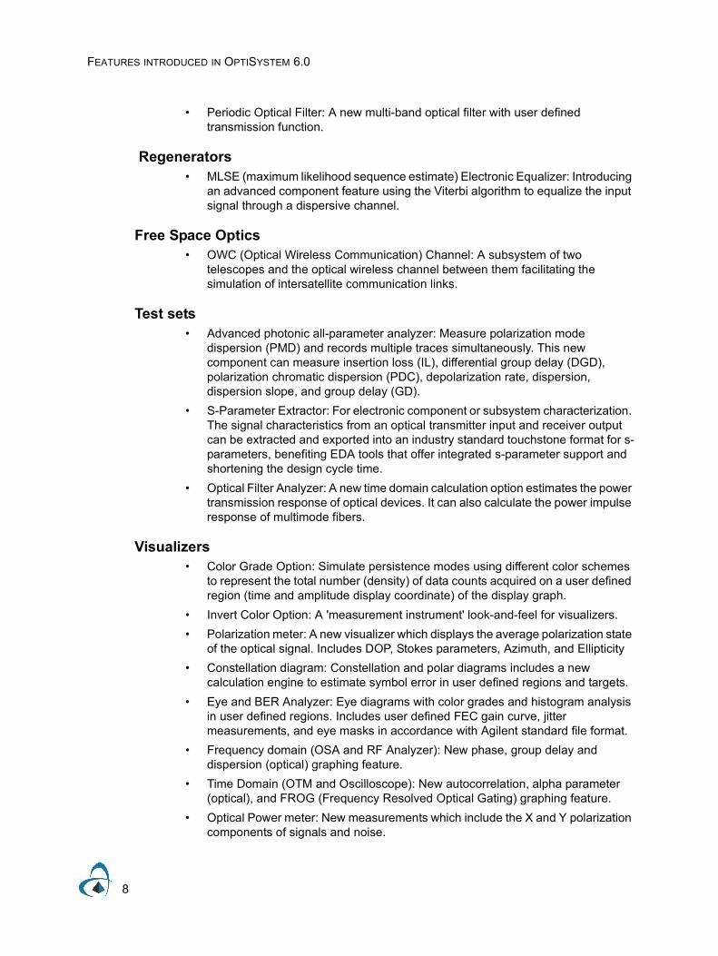
• Periodic Optical Filter: A new multi-band optical filter with user defined transmission function.

Regenerators• MLSE (maximum likelihood sequence estimate) Electronic Equalizer: Introducing

an advanced component feature using the Viterbi algorithm to equalize the input signal through a dispersive channel.

Free Space Optics• OWC (Optical Wireless Communication) Channel: A subsystem of two

telescopes and the optical wireless channel between them facilitating the simulation of intersatellite communication links.

Test sets• Advanced photonic all-parameter analyzer: Measure polarization mode

dispersion (PMD) and records multiple traces simultaneously. This new component can measure insertion loss (IL), differential group delay (DGD), polarization chromatic dispersion (PDC), depolarization rate, dispersion, dispersion slope, and group delay (GD).

• S-Parameter Extractor: For electronic component or subsystem characterization. The signal characteristics from an optical transmitter input and receiver output can be extracted and exported into an industry standard touchstone format for s-parameters, benefiting EDA tools that offer integrated s-parameter support and shortening the design cycle time.

• Optical Filter Analyzer: A new time domain calculation option estimates the power transmission response of optical devices. It can also calculate the power impulse response of multimode fibers.

Visualizers• Color Grade Option: Simulate persistence modes using different color schemes

to represent the total number (density) of data counts acquired on a user defined region (time and amplitude display coordinate) of the display graph.

• Invert Color Option: A 'measurement instrument' look-and-feel for visualizers.• Polarization meter: A new visualizer which displays the average polarization state

of the optical signal. Includes DOP, Stokes parameters, Azimuth, and Ellipticity • Constellation diagram: Constellation and polar diagrams includes a new

calculation engine to estimate symbol error in user defined regions and targets.• Eye and BER Analyzer: Eye diagrams with color grades and histogram analysis

in user defined regions. Includes user defined FEC gain curve, jitter measurements, and eye masks in accordance with Agilent standard file format.

• Frequency domain (OSA and RF Analyzer): New phase, group delay and dispersion (optical) graphing feature.

• Time Domain (OTM and Oscilloscope): New autocorrelation, alpha parameter (optical), and FROG (Frequency Resolved Optical Gating) graphing feature.

• Optical Power meter: New measurements which include the X and Y polarization components of signals and noise.


9

• Electrical Power meter: New measurements which include the AC and DC components of signals and noise.

GUI and Integrated Design Environment:• Display Results: Users can now select results to be displayed in the layout.

Results can be set to trigger alarms indicating if a result is out of a pre-defined range. Improved Project Browser to setup and display results.

• Project Export: Export current list of components, parameters and results directly to Excel. Includes the option to export an OptiSystem file directly to a compressed file format.

• Memory Management: Enable/disable signal monitors and graphs to save memory when using large number of iteration sweeps.

• Nested Parameter Sweeps: In addition to the standard OptiSystem parallel sweep and the script editor, OptiSystem supports nested parameter sweeps. Combined with the report page, users can easily build 2D and 3D graphs using different nesting levels.

• Component Viewer: The new component viewer allows for easy access to component results and graphs.

• Component Script: Write your own calculation engine. For example, a new result can be added to a component or visualizer, offering unlimited possibilities in terms of post-processing. Script can access component parameters, results and graphs.


10

Notes:

11

IntroductionOptical communication systems are increasing in complexity on an almost daily basis. The design and analysis of these systems, which normally include nonlinear devices and non-Gaussian noise sources, are highly complex and extremely time-intensive. As a result, these tasks can now only be performed efficiently and effectively with the help of advanced new software tools.

OptiSystem is an innovative optical communication system simulation package that designs, tests, and optimizes virtually any type of optical link in the physical layer of a broad spectrum of optical networks, from analog video broadcasting systems to intercontinental backbones.

OptiSystem is a stand-alone product that does not rely on other simulation frameworks. It is a system level simulator based on the realistic modeling of fiber-optic communication systems. It possesses a powerful new simulation environment and a truly hierarchical definition of components and systems. Its capabilities can be extended easily with the addition of user components, and can be seamlessly interfaced to a wide range of tools.

A comprehensive Graphical User Interface (GUI) controls the optical component layout and netlist, component models, and presentation graphics (see Figure 1 on page 18).

The extensive library of active and passive components includes realistic, wavelength-dependent parameters. Parameter sweeps allow you to investigate the effect of particular device specifications on system performance.

Created to address the needs of research scientists, optical telecom engineers, system integrators, students, and a wide variety of other users, OptiSystem satisfies the demand of the booming photonics market for a powerful and easy-to-use optical system design tool.

OptiSystem is also available in two additional configurations:• Amplifier Edition• Multimode Edition

INTRODUCTION

12

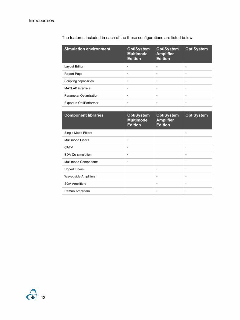
The features included in each of the these configurations are listed below.

Simulation environment OptiSystem Multimode Edition

OptiSystem Amplifier Edition

OptiSystem

Layout Editor • • •

Report Page • • •

Scripting capabilities • • •

MATLAB interface • • •

Parameter Optimization • • •

Export to OptiPerformer • • •

Component libraries OptiSystem Multimode Edition

OptiSystem Amplifier Edition

OptiSystem

Single Mode Fibers •

Multimode Fibers • •

CATV • •

EDA Co-simulation • •

Multimode Components • •

Doped Fibers • •

Waveguide Amplifiers • •

SOA Amplifiers • •

Raman Amplifiers • •

INTRODUCTION

13

Benefits• Rapid, low-cost prototyping• Global insight into system performance• Straightforward access to extensive sets of system characterization data• Automatic parameter scanning and optimization• Assessment of parameter sensitivities aiding design tolerance specifications• Dramatic reduction of investment risk and time-to-market• Visual representation of design options and scenarios to present to prospective

customers

ApplicationsOptiSystem allows for the design automation of virtually any type of optical link in the physical layer, and the analysis of a broad spectrum of optical networks, from long-haul systems to MANs and LANs.

OptiSystem’s wide range of applications include:• Optical communication system design from component to system level at the

physical layer• CATV or TDM/WDM network design• Passive optical networks (PON) based FTTx• Free space optic (FSO) systems• Radio over fiber (ROF) systems• SONET/SDH ring design• Transmitter, channel, amplifier, and receiver design• Dispersion map design• Estimation of BER and system penalties with different receiver models• Amplified system BER and link budget calculations

INTRODUCTION

14

Main featuresThe main features of the OptiSystem interface include:

Feature Description

Component Library To be fully effective, component modules must be able to reproduce the actual behavior of the real device and specified effects according to the selected accuracy and efficiency. The OptiSystem Component Library includes hundreds of components, all of which have been carefully validated in order to deliver results that are comparable with real life applications.

Measured components The OptiSystem Component Library allows you to enter parameters that can be measured from real devices. It integrates with test and measurement equipment from different vendors.

Integration with Optiwave Software Tools

OptiSystem allows you to employ specific Optiwave software tools for integrated and fiber optics at the component level: OptiAmplifier, OptiBPM, OptiGrating, WDM_Phasar, and OptiFiber.

Mixed signal representation

OptiSystem handles mixed signal formats for optical and electrical signals in the Component Library. OptiSystem calculates the signals using the appropriate algorithms related to the required simulation accuracy and efficiency.

Quality and performance algorithms

In order to predict the system performance, OptiSystem calculates parameters such as BER and Q-Factor using numerical analysis or semi-analytical techniques for systems limited by inter symbol interference and noise.

Advanced visualization tools

Advanced visualization tools produce OSA Spectra, signal chirp, eye diagrams, polarization state, constellation diagrams and much more. Also included are WDM analysis tools listing signal power, gain, noise figure, and OSNR per channel.

Data monitors You can select component ports to save the data and attach monitors after the simulation ends. This allows you to process data after the simulation without recalculating. You can attach an arbitrary number of visualizers to the monitor at the same port.

Hierarchical simulation with subsystems

To make a simulation tool flexible and efficient, it is essential to provide models at different abstraction levels, including the system, subsystem, and component levels. OptiSystem features a truly hierarchical definition of components and systems, enabling you to employ specific software tools for integrated and fiber optics at the component level, and allowing the simulation to be as detailed as the desired accuracy dictates.

INTRODUCTION

15

User-defined components

You can incorporate new components based on subsystems and user-defined libraries, or use co-simulation with a third party tool such as MATLAB.

Powerful Script language You can enter arithmetical expressions for parameters and create global parameters that can be shared between components and subsystems using standard VB Script language. The script language can also manipulate and control OptiSystem, including calculations, layout creation and post-processing when using the script page.

State-of-the-art calculation data-flow

The Calculation Scheduler controls the simulation by determining the order of execution of component modules according to the selected data flow model. The main data flow model that addresses the simulation of the transmission layer is the Component Iteration Data Flow (CIDF). The CIDF domain uses run-time scheduling, supporting conditions, data-dependent iteration, and true recursion.

Multiple layouts You can create many designs using the same project file, which allows you to create and modify your designs quickly and efficiently. Each OptiSystem project file can contain many design versions. Design versions are calculated and modified independently, but calculation results can be combined across different versions, allowing for comparison of the designs.

Report page A fully customizable report page allows you to display any set of parameters and results available in the design. The produced reports are organized into resizable and moveable spreadsheets, text, 2D and 3D graphs. It also includes HTML export and templates with pre-formatted report layouts.

Parameter sweeps and optimizations

Simulations can be repeated with an iterated variation of the parameters. OptiSystem can also optimize any parameter to minimize or maximize any result or can search for target results. You can combine multiple parameter sweeps and multiple optimizations.

OptiPerformer For any given system topology and component specification scenario, a full OptiSystem project can be encrypted and exported to OptiPerformer. OptiPerformer users can then vary any parameter within defined specification ranges, and observe resulting system effects via detailed graphics and reports.

Bill of materials OptiSystem provides a cost analysis table of the system being designed, arranged by system, layout or component. Cost data can be exported to other applications or spreadsheets.

Feature Description

INTRODUCTION

16

Notes:

QUICK START

17

Quick StartThis section describes how to load a design, run a simulation, edit local and global parameters, and obtain results. The most efficient way to become familiar with OptiSystem is to complete the lessons in the Tutorials, where you learn how to use the software by solving problems.

Note: For the users of the Amplifier Edition of OptiSystem we recommend to follow Lesson 7: Optical Amplifiers - Designing optical fiber amplifiers and fiber lasers, and for the users of the Multimode Edition of OptiSystem we recommend to follow Lesson 8: Optical Systems - Working with multimode components. Both lessons are available in the OptiSystem tutorials book.

Starting OptiSystemTo start OptiSystem, perform the following action.

Action • From the Start menu, select Programs > Optiwave Software>

OptiSystem 7 > OptiSystem.OptiSystem loads and the graphical user interface appears(see Figure 1).

QUICK START

18

Figure 1 OptiSystem graphical user interface (GUI)

QUICK START

19

Main parts of the GUIThe OptiSystem GUI contains the following main windows:• Project layout• Dockers

— Component Library

— Project Browser

— Description

• Status Bar

Project layoutThe main working area where you insert components into the layout, edit components, and create connections between components (see Figure 2).

Figure 2 Project layout window

QUICK START

20

DockersUse dockers, located in the main layout, to display information about the active (current) project:

— Component Library

— Project Browser

— Description

Component LibraryAccess components to create the system design (see Figure 3).

Figure 3 Component Library window

Project BrowserOrganize the project to achieve results more efficiently, and navigate through the current project (see Figure 4).

Figure 4 Project Browser window

QUICK START

21

Description

Display detailed information about the current project (see Figure 5).

Figure 5 Description window

Status BarDisplays project calculation progress information, useful hints about using OptiSystem, and other help. Located at the bottom of the Project Layout window.

Figure 6 Status Bar

QUICK START

22

Loading a sample file

To load a sample file, perform the following procedure.

Step Action 1 From the File menu, select Open.

2 In Samples > Introductory Tutorials, select Quick Start Direct Modulation.osd.The Direct Modulation sample file appears in the Main layout (see Figure 7).

Figure 7 Direct Modulation sample file

The transmitter is built using a direct laser modulation scheme, and consists of the following components:• Pseudo-Random Bit Sequence Generator: Sends the bit sequence to the NRZ

Pulse Generator. The pulses modulate the Laser Measured. The Photodetector PIN receives the optical signal attenuated by the Optical Attenuator. The Low Pass Bessel Filter filters the electrical signal.

• Optical Spectrum Analyzer: Displays the modulated optical signal in the frequency domain

QUICK START

23

• Optical Time Domain Visualizer: Displays the modulated optical signal in the time domain.

• Oscilloscope Visualizer: Displays the electrical signal after the PIN in time domain.

• BER Analyzer: Measures the performance of the system based on the signal before and after the propagation.Note: More than one visualizer can be attached to a component output.

Running a simulation

To run a simulation, perform the following procedure.

Step Action 1 From the File menu, select Calculate (see Figure 8).

The OptiSystem Calculations dialog box appears (see Figure 9).

Figure 8 File menu

QUICK START

24

Figure 9 OptiSystem Calculations dialog box

2 In the OptiSystem Calculations dialog box, click the Run button (see Figure 9).The results appear in the Calculation Output window.The calculation output appears in the Calculation Output window, and the simulation results appear below the components that were included in the simulation.

QUICK START

25

Displaying results from a visualizer

To view the simulation results, perform the following action.

Action • Double-click a visualizer in the Project layout to view the graphs and results

that the simulation generates (see Figure 10).

Figure 10 Optical Time Domain Visualizer results

QUICK START

26

Component parameters

Viewing and editing component parameters

Double-click a component to view and edit the parameters for the component. To view the properties for Laser Measured, perform the following action.

Action • In the Project layout, double-click the Laser Measured component.

The Laser Measured Properties dialog box appears.

Figure 11 Component parameters – Laser Measured

QUICK START

27

Component parameters are organized by categories. Laser Measured has seven parameter categories, each represented by a tab in the dialog box (see Figure 11).• Main• Measurements• Physical• Initial estimate• Simulation• Noise• Random numbers

Each category has a set of parameters. Parameters have the following properties:• Disp• Name• Value• Units• Mode

The first category in the Laser Measured dialog box is Main. You can enter the signal Frequency and Power using the Main tab.

The first parameter in the Main category is Disp. When you select a check box beside a parameter listed in the Disp column, the parameter value appears under the component in the Project layout. For example, if you select the Frequency and Power check boxes in the Disp column, these parameter values appear in the Project layout (see Figure 12).

Figure 12 Laser Measured with displayed parameter values

Each parameter can have a value in the columns Name, Value, Units, and Mode. Some parameters can have different units. For example, you can select the Frequency parameter to be in Hz, THz, or nm. When you change your unit selection, the conversion is automatic (see Figure 13).

QUICK START

28

Figure 13 Choosing parameter values

QUICK START

29

Editing parametersTo edit the NRZ Pulse Generator parameters, perform the following procedure.‘

Step Action 1 Double-click the NRZ Pulse Generator in the Project layout.

The NRZ Pulse Generator Properties dialog box appears (see Figure 14).

2 Click the Simulation tab.

Figure 14 Laser NRZ Pulse Generator simulation options

QUICK START

30

For the Sample rate parameter, the Mode is Script (see Figure 15). This parameter will be evaluated as an arithmetic expression. The Sample rate parameter of the Laser Measured component also refers to a Global parameter with the same name.

Figure 15 Scripted parameters

QUICK START

31

Editing visualizer parameters

To access the parameters for the Optical Spectrum Analyzer, perform the following procedure.

Step Action 1 Right-click the Optical Spectrum Analyzer.

A shortcut menu appears (see Figure 16).

Figure 16 Shortcut menu

Select Component Properties.The Optical Spectrum Analyzer Properties dialog box appears (see Figure 17).

QUICK START

32

Figure 17 Optical Spectrum Analyzer Properties dialog box

QUICK START

33

Global parametersThe global parameters are common to all OptiSystem simulations. (See Appendix A: Global Parameters for more information on global parameters.) In this particular case, you indirectly define the simulation time window, the number of samples, and the sample rate using three parameters:• Bit rate• Bit sequence length• Number of samples per bit

These parameters are used to calculate the Time window, Sample rate, and Number of samples.• Time window = Sequence length * 1/Bit rate = 256 * 1 / 10e9 = 25.6 ns• Number of samples = Sequence length * Samples per bit = 32768 samples• Sample rate = Number of samples / Time window = 1.28 THz

The time window of the simulation is 25.6 ns. 32768 samples will be generated by each component, and the signal bandwidth is 1.28 THz.

OptiSystem shares the parameter Time window with all components. This means that each component works with the same time window. However, each component can work with different sample rates or number of samples (see Figure 18).

QUICK START

34

Figure 18 Global parameters values

QUICK START

35

Editing global parameters

To edit global parameters, perform the following procedure.

Step Action 1 Double-click in the Project layout.

The Layout 1 Parameters dialog box appears (see Figure 18).

2 Select or clear global parameters as required.

These parameters can be accessed by any component using the script mode. The NRZ Pulse Generator refers by default to the global parameter Sample rate using script mode (see Figure 19). The Low Pass Bessel Filter has the Cutoff parameter frequency as 0.75 * Bit rate. In this case, Bit rate is a global parameter (see Figure 20).

Figure 19 NRZ Pulse Generator properties

QUICK START

36

Figure 20 Low Pass Bessel Filter properties

QUICK START

37

Using the Layout Editor

In the following example, you will modify a design that you create. You will change the laser modulation scheme from direct to external modulation by replacing some of the components in the design and adding components from the Component Library.

To use the Layout Editor, perform the following procedure.

Step Action 1 To delete the Laser Measured component, select the Laser Measured

component in the Project layout and press the Delete key.The Laser Measured component is deleted from the layout.

2 From the Component Library, select Default > Transmitters Library > Optical Sources.

3 Drag the CW Laser to the Project layout (see Figure 21).

Note: The autoconnect feature automatically connects components in the Project layout. If connections are not made automatically, see “Connecting components manually” on page 39.

Figure 21 CW Laser added to Main Layout

QUICK START

38

4 From the Component Library, select Default > Transmitters Library > Optical Modulators.

5 Drag the Mach-Zehnder Modulator to the Project layout (see Figure 22).

6 Place the Mach-Zehnder Modulator in the Project layout so the following connections are generated:

a. NRZ Pulse Generator output port to the Mach-Zehnder modulation input port

b. CW Laser output port to the Mach-Zehnder Modulator Carrier input port

c. Mach-Zehnder Modulator output port to the Optical Attenuator input port

Figure 22 Connecting components

7 Connect the Mach-Zehnder Modulator output port to the Optical Spectrum Analyzer input port and to the Optical Time Domain Visualizer input port (see Figure 23).

QUICK START

39

Figure 23 Mach-Zehnder Modulator connected to visualizers

8 From the File menu, select Calculate.The OptiSystem Calculations dialog box appears.

9 Click the Run button.The results appear in the Calculation Output window.

10 To view the graphs and results, double-click on the visualizers (see Figure 25 and Figure 26 for examples of visualizer results).

Connecting components manually

To connect components using the layout tool, perform the following procedure.

Step Action 1 Place the cursor over the initial port.

The cursor changes to the rubber band cursor (chain link) (see Figure 24).A tool tip appears that indicates the type of signal that is available on this port.

2 Click and drag to the port to be connected.The ports are connected.

Note: You can only connect output to input ports and vice versa.

Figure 24 Rubber Band cursor

QUICK START

40

Figure 25 Visualizer results — OSA example

QUICK START

41

Figure 26 Visualizer results — BER example

Saving the design and closing OptiSystem

To save the design and close OptiSystem, perform the following procedure.

Step Action 1 From the File menu, select Save.

The Quick Start Direct Modulation.osd design is saved.

2 From the File menu, select Exit.OptiSystem closes.

QUICK START

42

Notes:

APPENDIX A: GLOBAL PARAMETERS

43

Appendix A: Global ParametersOpening the global parameters dialog

To open the global parameters dialog, perform the following action.

Action • Double-click in the Project layout window.

The Layout Parameters dialog opens (see Figure 27).OR

• Select Layout > Parameters from the Menu tool bar.The Layout Parameters dialog opens (see Figure 27).

Editing global parametersTo edit global parameters, perform the following procedure.

Step Action 1 Double-click in the Project layout.

The Layout Parameters dialog box appears (see Figure 27).

2 Select or clear global parameters as required.


44

Figure 27 Layout Parameters dialog


45

When you create a new design, you must define the global simulation parameters. These parameters are critical to the simulation.

They show the speed, accuracy, and memory requirements for a particular simulation during the system design stage. It is important to understand what the global parameters are, because they have an impact on all the components that use these parameters (see Figure 28).

Figure 28 Global parameters relationships

Time spacing = 1 / Sample rate = Time window / Number of samples

Frequency spacing - 1 / Time window - Sample rate / Number of samples

Time window = Sequence length * Bit period - Sequence length / Bit rate

Number of samples - Sequence length * Samples per bit - Time window * Sample rate


46

Simulation parameters

Figure 29 Simulation parameters

Simulation windowSpecifies the setup mode for entering the parameters that define the main simulation parameters:• Set bit rate: Allows you to enter the Bit rate. This is the default mode — you can

easily set up the simulation using typical parameters such as Bit rate, Sequence length, and Samples per bit.

• Set time window: Allows you to enter the Time window value• Set sample rate: Allows you to enter the Sample rate

The parameter Bit rate recalculates based on these parameters.


47

Reference bit rateIf this parameter is enabled, when you select Set time window or Set sample rate in the Simulation window, it will find the closest Time window or Sample rate without changing the Bit rate.

Bit rateThe value of the global bit rate is in bits per second. All components can access this parameter (see Figure 30). The global bit rate can affect components such as Bit sequence generators because components that require this parameter use is as a default value.

An expression relative to this bit rate value is used to define the default value for the bandwidth or cutoff frequency of most electrical filters. When you change this global parameter, you can change the bit rate setting of all modules in the design simultaneously.

Figure 30 Global parameter Bit rate

Bit rate


48

Time windowSpecifies in seconds the Time window of the simulation. OptiSystem shares the parameter Time window with all components. This means that each component works with the same Time window. Since the Time window defines the frequency spacing in the frequency domain, the sampled signal will always have the same frequency spacing. This parameter is best expressed in terms of the sequence length and the bit rate used during the simulation. It affects all components.

Sample rateSpecifies the frequency simulation window or simulation bandwidth in Hz (see Figure 31). It can affect components such as pulse generators and optical sources that generate signals at different sample rates. It is often convenient to operate all modules in the design at the same sample rate. This can be done easily by using this global parameter. The default parameter for all components requiring sample rate is referred to as the global sample rate. When you change this global parameter, you can change the sample rate setting of all modules in the design simultaneously.

Figure 31 Global parameter Sample rate


49

Sequence lengthThe length of the bit sequence in number of bits. It must be a power of two.

Figure 32 Global parameter Sequence length

Samples per bitNumber of samples for bit used to discretize the sampled signals. It must be a power of two.

Number of samplesThis read-only parameter shows the number of samples calculated by the product of Sequence length and Samples per bit.

Sequence length


50

Figure 33 Global parameter iterations


51

Signals parameters

Figure 34 Global parameters Signals


52

IterationsNumber of signal blocks generated by each simulation. It mainly affects transmitters and components used in bidirectional simulations and in network ring design.

By increasing the parameter iterations a component will repeat the previous calculation until the number of calculations is equal to the iterations. Refer to the tutorial lesson: Working with multiple iterations.

Initial DelayThis parameter forces a component to generate a null signal at each output port. It affects all components and it is mainly used in bidirectional simulations. The user does not have to add delays at the component input ports if using this parameter. Refer to the tutorial lesson: Working with multiple iterations.

ParameterizedDefines whether the signal output will be sampled signals (disabled) or parameterized signals (enabled). It can affect components such as optical sources and optical pulse generators.

SynchronizeDefines whether bit rates will be recalculated in order to make sure that the number of samples and the number of bits are both power of two numbers. It can affect components such as pulse generators, decoders and BER analyzers. It forces compatibility mode with previous versions of OptiSystem 7.


53

Noise parameters

Convert noise binsSelects whether noise within a sampled band's frequency range is added to the sampled signal or represented separately as noise bins. The default value is disabled, which means the noise propagate is separated from the signals. It can affect the Erbium doped fiber amplifiers and the photo detectors.

Figure 35 Global parameters Noise


54

Spatial Effects ParametersThe spatial effects parameters affect the components that generate spatial modes, where the discretization space and the level of the discretization should be defined. The number of points per spatial mode is defined as the product of the number of points in the X and Y coordinates.

Figure 36 Global spatial effects parameters

Space Width XThis is the space for the X coordinate.

Space Width YThis is the space for the Y coordinate.


55

Grid Spacing Width XThe grid spacing for the X coordinate. The space width divided by the grid spacing gives the number of points in the X coordinate.

Grid Spacing Width YThe grid spacing for the Y coordinate. The space width divided by the grid spacing gives the number of points in the Y coordinate

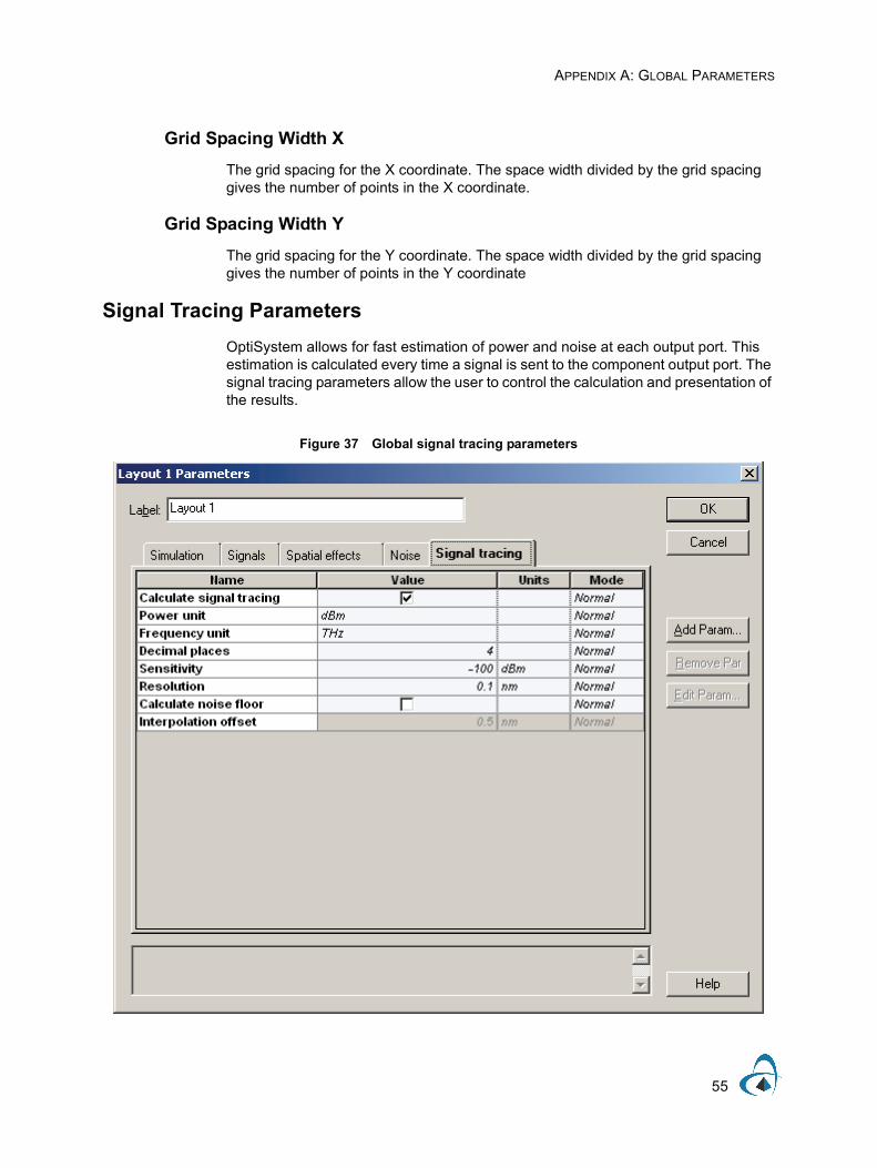
Signal Tracing ParametersOptiSystem allows for fast estimation of power and noise at each output port. This estimation is calculated every time a signal is sent to the component output port. The signal tracing parameters allow the user to control the calculation and presentation of the results.

Figure 37 Global signal tracing parameters


56

Calculate Signal TracingDefines if the signal will be traced.

Power UnitThe units used to display the results (dBm, W or mW).

Frequency UnitThe units used to display the results (Hz, m, THZ or nm).

Decimal PlacesThe number of decimal places to use when displaying the results.

SensitivityThe minimum output power that the calculation can detect.

ResolutionThe spectral resolution bandwidth of the calculation.

Calculate Noise FloorDefines if the noise floor will be calculated using interpolation. This is an important parameter when the noise is added to the signal.

Interpolation OffsetThe interpolation offset from the signal channel center frequency used to estimate the noise floor.

APPENDIX B: SIGNAL REPRESENTATION

57

Appendix B: Signal representationTo make the simulation tool more flexible and efficient, it is essential that it provides models at different abstraction levels, including the system, subsystem, and component levels. OptiSystem features a hierarchical definition of components and systems, allowing you to employ specific software tools for integrated and fiber optics in the component level and allowing the simulation to go as deep as the desired accuracy requires. Different abstraction levels imply different signal representations. The signal representation must be as complete as possible in order to allow efficient simulation.

There are five types of signals in the signal library:

Figure 38 Signal types and connections

Signal Connection color

Binary Red

M-Ary Dark Red

Electrical Blue

Optical Green

Any Type Dark Green


58

OptiSystem handles mixed signal formats in the Component Library for optical and electrical signals. It calculates the signals using different algorithms according to the desired simulation accuracy and efficiency.

Binary signalsBinary signals are generated by components such as bit sequence generators. Pulse generators in the Transmitters Library and digital switches in the Network Library use this signal as input data.

A binary signal consists of a sequence of ones and zeros, or marks and spaces. The main property of the binary signal is the Bit rate (see Figure 39).

Figure 39 Binary signal

M-Ary SignalsM-Ary signals are multilevel signals used for special types of coding, such as PAM, QAM, PSK, and DPSK. M-Ary signals are similar to the binary signals. However, M-Ary signals can have any level instead of only high (1) and low (0) levels, or marks and spaces. Refer to the digital modulation tutorial lessons.

Electrical signalsElectrical signals are generated by components such as pulse generators in the Transmitters Library and photodetectors in the Receivers Library.

Electrical signals consist of the sampled signal waveform in time domain. The main properties of the electrical signal are the signal noise variances in the time domain and the noise power spectral densities in the frequency domain.


59

When a pulse generator generates the electrical signal, there is no noise information with the signal because the signal is pure. If the electrical signal is generated by a photodetector, there are different sources of noise, some of which are time dependent and must be characterized by the time variance (for example, shot noise). Some of them are given as power spectral density (for example, thermal noise). The electrical signal creates the noise information according to the properties and the number of noise sources in the component (see Figure 40).

Figure 40 Electrical signal - noise variance - PSD

If the electrical signal is filtered, the noise PSD is affected immediately because the PSD is filtered based on the filter transfer function in frequency domain. If the noise is also characterized by the noise variance, it is not affected immediately. The information about the filter transfer function is saved in the frequency domain as a property of the noise. As a result, you can have a cascade of electrical filters and the electrical signal will keep track of the equivalent transfer function of the filters.

When using the noise variance for calculation of the signal noise, the information about the filters will be used to generate the equivalent noise bandwidth and will be applied to the noise variance (see Figure 41).

Electrical signals can also be represented by individual samples, allowing for time driven simulations. In order to simulate using individual samples the user should explicitly add the component “Convert to Individual Electrical Samples" into the layout. The signal and noise at the input signal will be added and converted into multiple samples. The number of samples is defined by the global parameter Number of samples. Refer to the tutorial lesson: Working with individual samples.


60

Figure 41 Filtering electrical signal

Optical signalsOptical signals are generated by components such as lasers in the Transmitters Library. Optical signals accommodate different signal representations:• Sampled signals• Parameterized signals• Noise bins

Figure 42 Mixed optical signal representation - Frequency domain


61

Sampled signalsOptical signals can accommodate any arbitrary number of signal bands. In the simplest case, there is one single frequency band when a single, continuous frequency band represents the waveforms of all the modulated optical carriers. A single optical source (for example, CW Laser) produces a single frequency band. The band represents the complex sampled optical field of the signal in two polarizations. This type of optical signal is called a Sampled signal.

When two or more Sampled signals are combined, the individual signals will join into a new sampled signal if their simulation bandwidths overlap, or they are kept separated if the simulation bandwidth does not overlap. The resulting signal is called Sampled signals — in this case, each sampled signal is propagated using a separate sampled optical field.

Example

Signals are generated in each laser and are combined in the multiplexer. After the multiplexer, the channels at frequencies 193.1 and 193.2 THz overlap, so they are added to the same band (see Figure 43).

Sampled signals can also have spatial representation for the spatial modes. If you are using the multimode component library, the sampled signals will also have the spatial distribution of the signal power for both polarizations.

Optical signals can also be represented by individual samples, allowing for time-driven simulations. In order to simulate using individual samples, the user should explicitly add the component "Convert to Individual Optical Samples" into the layout. Only sampled signals can be converted into individual samples. The number of individual samples is defined by the global parameter Number of samples. If the input signal has multiple channels, each channel will have an individual sample and center frequency, allowing for WDM and Time-driven simulations. Refer to the tutorial lesson: Working with individual samples.


62

Figure 43 Overlapping channel frequencies

Parameterized signalsThe signal description based on the Sampled signals covers the majority of physical phenomena affecting the system design. When designing a system where the power budget analysis and the fast signal-to-noise ratio estimations are the main performance evaluation results, signal channels can be approximated by their average power, assuming that the detailed waveform of their data streams are not important. One application example is the investigation of the transmission behavior of the central channels in dense WDM systems, or an estimation of the EDFA performance in the steady-state regime.

Parameterized Signals are time-averaged descriptions of the sampled signals based on the information about the optical signal (for example, Average power, Central frequency, and Polarization state).

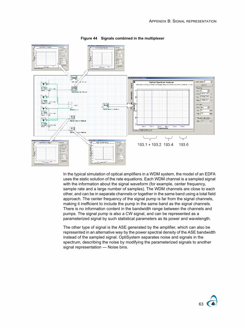
Example

Signals are generated in each laser using parameterized representation and combined in the multiplexer. Signals are represented by power and frequency (see Figure 44).


63

Figure 44 Signals combined in the multiplexer

In the typical simulation of optical amplifiers in a WDM system, the model of an EDFA uses the static solution of the rate equations. Each WDM channel is a sampled signal with the information about the signal waveform (for example, center frequency, sample rate and a large number of samples). The WDM channels are close to each other, and can be in separate channels or together in the same band using a total field approach. The center frequency of the signal pump is far from the signal channels, making it inefficient to include the pump in the same band as the signal channels. There is no information content in the bandwidth range between the channels and pumps. The signal pump is also a CW signal, and can be represented as a parameterized signal by such statistical parameters as its power and wavelength.

The other type of signal is the ASE generated by the amplifier, which can also be represented in an alternative way by the power spectral density of the ASE bandwidth instead of the sampled signal. OptiSystem separates noise and signals in the spectrum, describing the noise by modifying the parameterized signals to another signal representation — Noise bins.


64

Noise binsNoise bins represent the noise by the average spectral density in two polarizations using a coarse spectral resolution. The resolution can be adapted to maintain the accuracy of the simulation. The main advantage of using Noise bins is to cover the wide spectrum of the optical signals or to represent the noise outside the Sample signals bandwidths. The noise bin representation is similar to the parameterized signals, including the polarization. The main difference is that noise bins are defined by the noise power density and the bandwidth of each noise bin instead of by the average power (see Figure 45).

Figure 45 Noise bins generated by EDFA

Noise Bins can be created whenever there is a source of optical noise, such as optical amplifiers. You define the initial resolution and bandwidth of the noise (see Figure 46).


65

Figure 46 Mixed signals generated by EDFA

During transmission, the widths of the noise bins are adapted automatically to describe the filtering of the noise with a specified precision. The noise bins shrink in width as they propagate through the simulation in order to maintain the discretization accuracy (see Figure 47).


66

Figure 47 Filtering noise bins – adaptive band of each bin

Optiwave7 Capella CourtOttawa, Ontario, K2E 7X1, Canada

Tel.: 1.613.224.4700Fax: 1.613.224.4706

E-mail: [email protected]: www.optiwave.com

OptiSystem User Book - dru5cjyjifvrg.cloudfront.net · and fiber optic amplifiers. OptiSystem...

Documents

Transcript of OptiSystem User Book - dru5cjyjifvrg.cloudfront.net · and fiber optic amplifiers. OptiSystem...