Options Pricing Lecture 21

U.C. Berkeley© M. Spiegel and R. Stanton, 2000 1

Lecture 21Options Pricing

Lecture 21Options Pricing

■ Readings– BM, chapter 20– Reader, Lecture 21


OutlineOutline

■ Last lecture:– Examples of options– Derivatives and risk (mis)management– Replication and Put-call parity

■ This lecture– Binomial option valuation– Black Scholes formula


Put-Call parity and early exercisePut-Call parity and early exercise

■ Put-call parity:C = S + P – K / (1+r)T

■ Put-call parity gives us an important result aboutexercising American call options.

■ In words, the value of a European (and hence American)call is strictly larger than the payoff of exercising it today.

( )( )

.KSr1KS

r1KPSCT

T

−>+−≥

+−+=


Early ExerciseEarly Exercise

■ In the absence of dividends, you should thus never exercisean American call prior to expiration.– What should you do instead of exercising if you’re worried that

your currently “in-the-money” (S > K) option will expire “out-of-the-money” (S < K)?

– What is the difference between the value of a European and anAmerican call option?

■ Note: If the stock pays dividends, you might want toexercise the option just before a dividend payment.

■ Note: This only applies to an American call option.– You might want to exercise an American put option before

expiration, so you receive the strike price earlier.


Key Questions About DerivativesKey Questions About Derivatives

■ How should a derivative be valued relative to itsunderlying asset?

■ Can the payoffs of a derivative asset be replicated bytrading only in the underlying asset (and possibly cash)?– If we can find such a replicating strategy, the current value of the

option must equal the initial cost of the replicating portfolio.– This also allows us to create a non-existent derivative by following

its replicating strategy.

■ This is the central idea behind all of modern option pricingtheory.


NotationNotation

■ We shall be using the following notation a lot:

S = Value of underlying asset (stock)C = Value of call optionP = Value of put optionK = Exercise price of optionr = One period riskless interest rateR = 1 + r


Factors Affecting Option ValueFactors Affecting Option Value

■ The main factors affecting an option’s value are:

Factor Call PutS, stock price + -K, exercise price - +σ, Volatility + +T, expiration date (Am.) + +

T, expiration date (Eu.) + ? r + -

Dividends - +■ What is not on this list?


Binomial Option ValuationBinomial Option Valuation

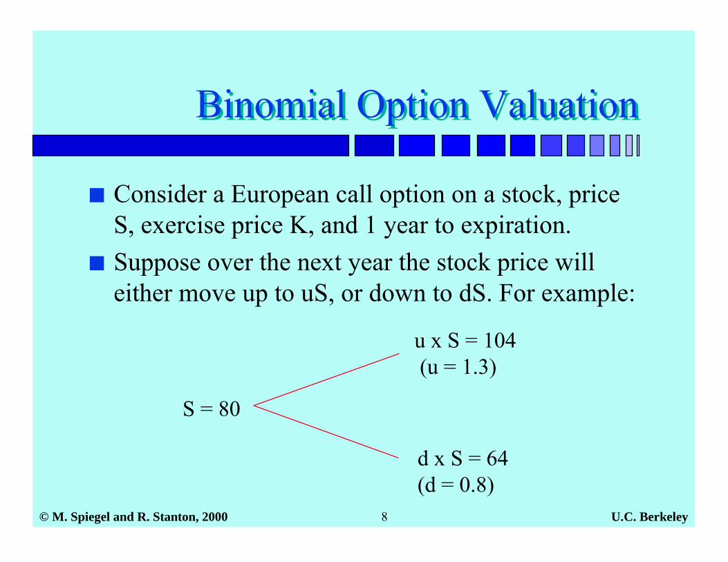
■ Consider a European call option on a stock, priceS, exercise price K, and 1 year to expiration.

■ Suppose over the next year the stock price willeither move up to uS, or down to dS. For example:

S = 80

u x S = 104 (u = 1.3)

d x S = 64(d = 0.8)


ExampleExample

■ Write C for the price of a call option today, and Cuand Cd for the price in one year in the two possiblestates, e.g. (suppose K = 90):

Cu = Max[104 – 90, 0] = 14

80

104

64

C

Stock Option

Cd = Max[64 – 90, 0] = 0


ExampleExample

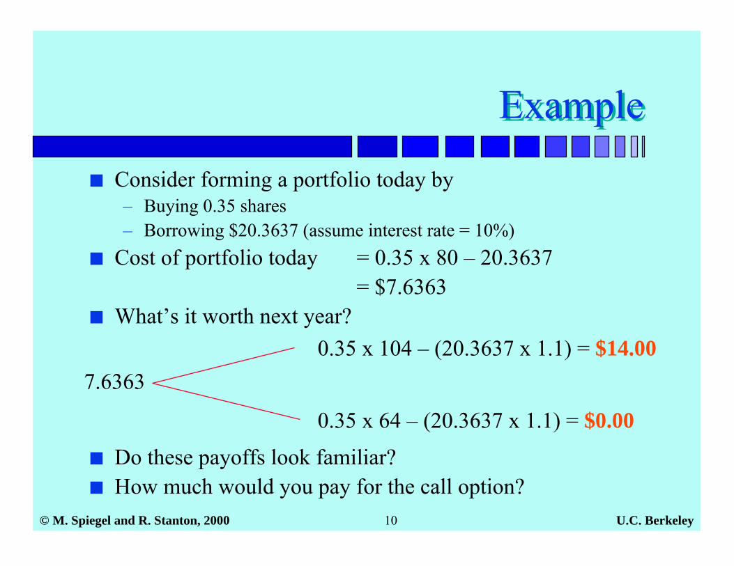
■ Consider forming a portfolio today by– Buying 0.35 shares– Borrowing $20.3637 (assume interest rate = 10%)

■ Cost of portfolio today = 0.35 x 80 – 20.3637= $7.6363

■ What’s it worth next year?

7.63630.35 x 104 – (20.3637 x 1.1) = $14.00

0.35 x 64 – (20.3637 x 1.1) = $0.00■ Do these payoffs look familiar?■ How much would you pay for the call option?


Replicating PortfoliosReplicating Portfolios

■ This is an example of a replicating portfolio.■ Its payoff is the same as that of the call option, regardless

of whether the stock goes up or down■ The current value of the option must therefore be the same

as the value of the portfolio, $7.6363– What if the option were trading for $5 instead?– Note that this result does not depend on the probability of an up vs.

a down movement in the stock price.

■ The call option is thus equivalent to a portfolio of theunderlying stock plus borrowing.

■ How do we construct the replicating portfolio in general?


Forming a Replicating Portfolioin General

Forming a Replicating Portfolioin General

■ Form a portfolio today by– Buying ∆ shares– Lending $B

■ Cost today = ∆S + B (= option price)■ Its value in one year depends on the stock price:

∆uS + B(1+r)

∆dS + B(1+r)

∆S + B


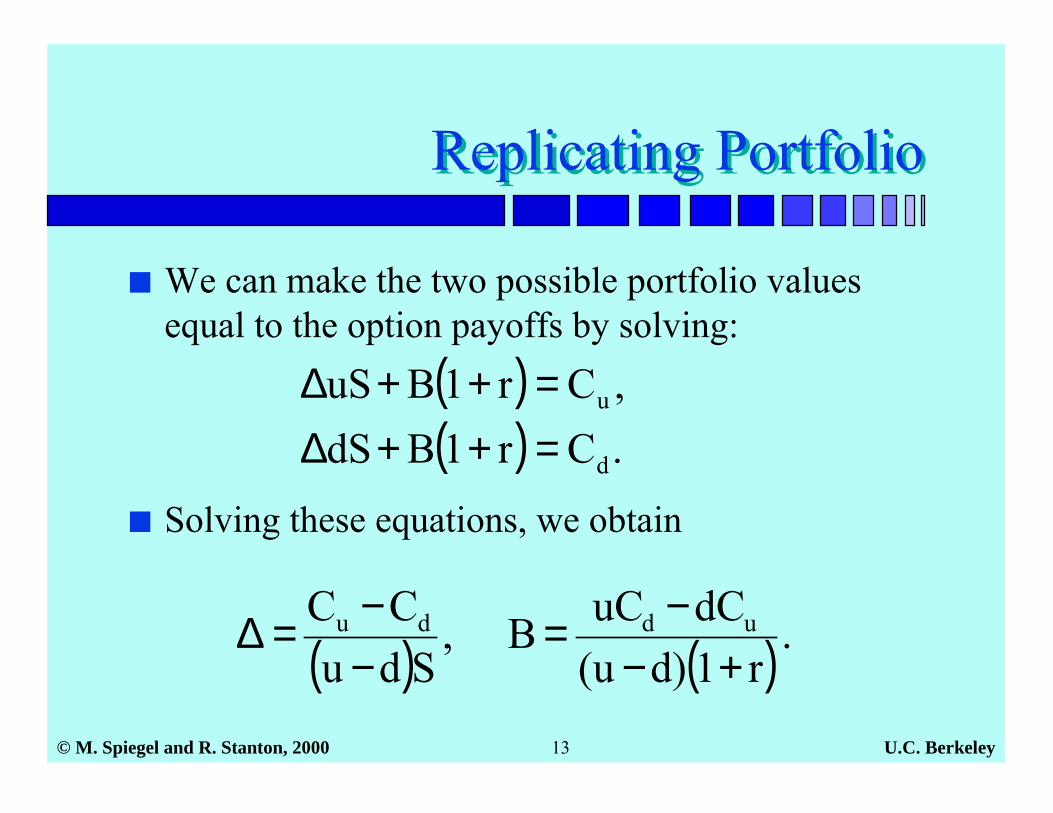
Replicating PortfolioReplicating Portfolio

■ We can make the two possible portfolio valuesequal to the option payoffs by solving:

( ) ( ).r1)du(

dCuCB,Sdu

CC uddu

+−−=

−−=∆

( )( ) .Cr1BdS

,Cr1BuS

d

u

=++∆=++∆

■ Solving these equations, we obtain


ExampleExample

■ S = 80, u = 1.3, d = 0.8■ K = 90, r = 10%.

80

104

64

C

Cu = 14

Cd = 0


ExampleExample

■ From the formulae,

( )( ) ( )

( ) .3637.201.18.03.1

148.003.1B

,35.0808.03.1

014

−=−−=

=−

−=∆

6363.7$3637.208035.0

BSC

=−×=

+∆=■ Hence


Delta and hedgingDelta and hedging

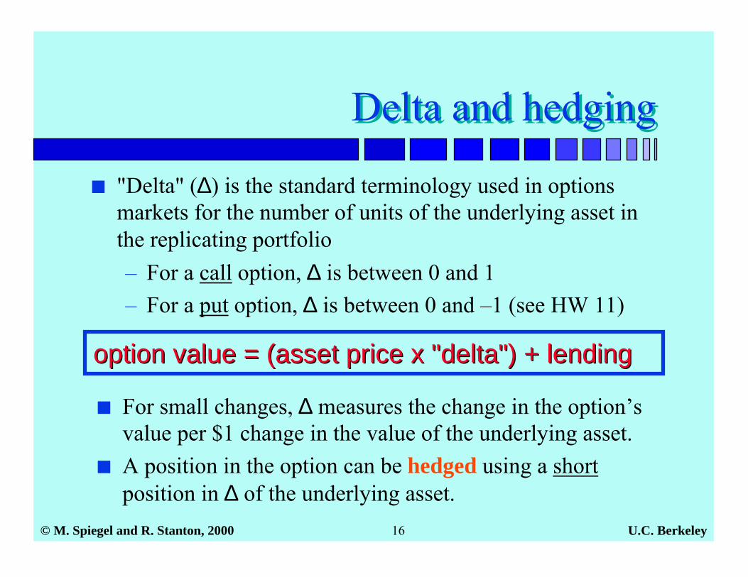
■ "Delta" (∆) is the standard terminology used in optionsmarkets for the number of units of the underlying asset inthe replicating portfolio– For a call option, ∆=is between 0 and 1– For a put option, ∆=is between 0 and –1 (see HW 11)

option value = (asset price x "delta") + lendingoption value = (asset price x "delta") + lending

■ For small changes, ∆ measures the change in the option’svalue per $1 change in the value of the underlying asset.

■ A position in the option can be hedged using a shortposition in ∆ of the underlying asset.


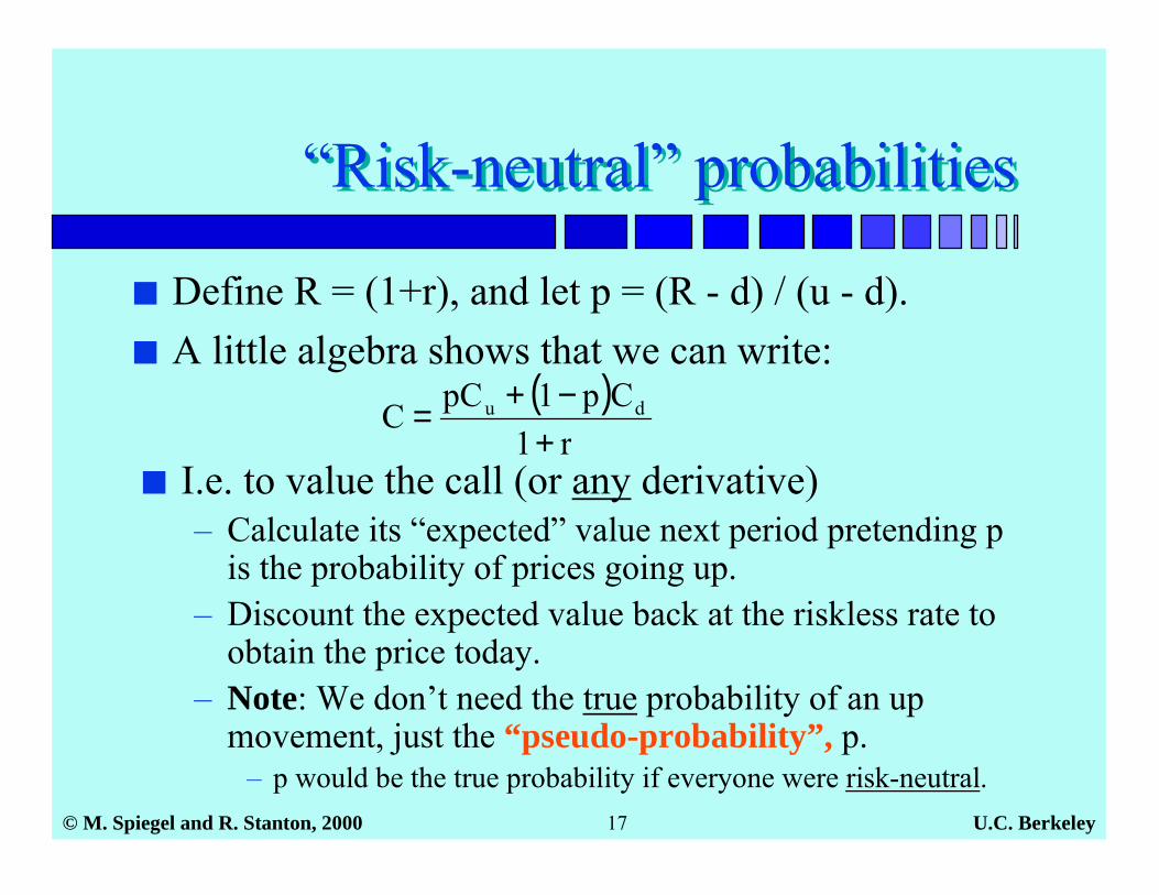
“Risk-neutral” probabilities“Risk-neutral” probabilities

■ Define R = (1+r), and let p = (R - d) / (u - d).■ A little algebra shows that we can write:

( )r1

Cp1pCC du

+−+=

■ I.e. to value the call (or any derivative)– Calculate its “expected” value next period pretending p

is the probability of prices going up.– Discount the expected value back at the riskless rate to

obtain the price today.– Note: We don’t need the true probability of an up

movement, just the “pseudo-probability”, p.– p would be the true probability if everyone were risk-neutral.


ExampleExample

■ Using the previous example,

■ Hence the call price equals

6.08.03.18.01.1

dudRp =

−−=

−−=

( )

( ) ( ) .6363.71.1

04.0146.0r1

Cp1pCC du

=×+×=

+−+=


Shortcomings of Binomial ModelShortcomings of Binomial Model

■ The binomial model provides many insights:– Risk neutral pricing– Replicating portfolio containing only stock + borrowing– Allows valuation/hedging using underlying stock

■ But it allows only two possible stock returns.■ To get around this:

– Split year into a number of smaller subintervals– Allow one up/down movement per subperiod– n subperiods give us n+1 values at end of year.


Example, two subperiodsExample, two subperiods

S

Su

Sd

Suu

Sud = Sdu

Sdd

■ Start at the end, and work backwards through tree.■ See reader pp. 164 – 167 for details.


How big should up/downmovements be?

How big should up/downmovements be?

■ For a given expiration date, we keep overallvolatility right as we split into n subperiods [eachof length t (= T/n)], by picking

■ As n gets larger, the distribution of the asset priceat maturity approaches a lognormal distribution,with expected return r, and annualized volatility σ.

■ What happens to option prices as we increase thenumber of time steps?

.eu1d,eu tσtσ −===


Binomial prices vs. # steps(S=K=60, T=0.5, σ=30%, r=8%)

Binomial prices vs. # steps(S=K=60, T=0.5, σ=30%, r=8%)

6

6.1

6.26.3

6.4

6.5

0 50 100 150 200 250Number of time steps

Valu

e of

cal

l opt

ion

What’s this limit?


Black-Scholes formulaBlack-Scholes formula

■ In the limit, the price of a European call optionconverges to the Black-Scholes formula,

■ r here is a continuously-compounded interest rate.

( ) ( )( ) ( )[ ]

tσtrKSlogxwhere

,tσxNKexNSC

2σ

rt

2++≡

−−= −


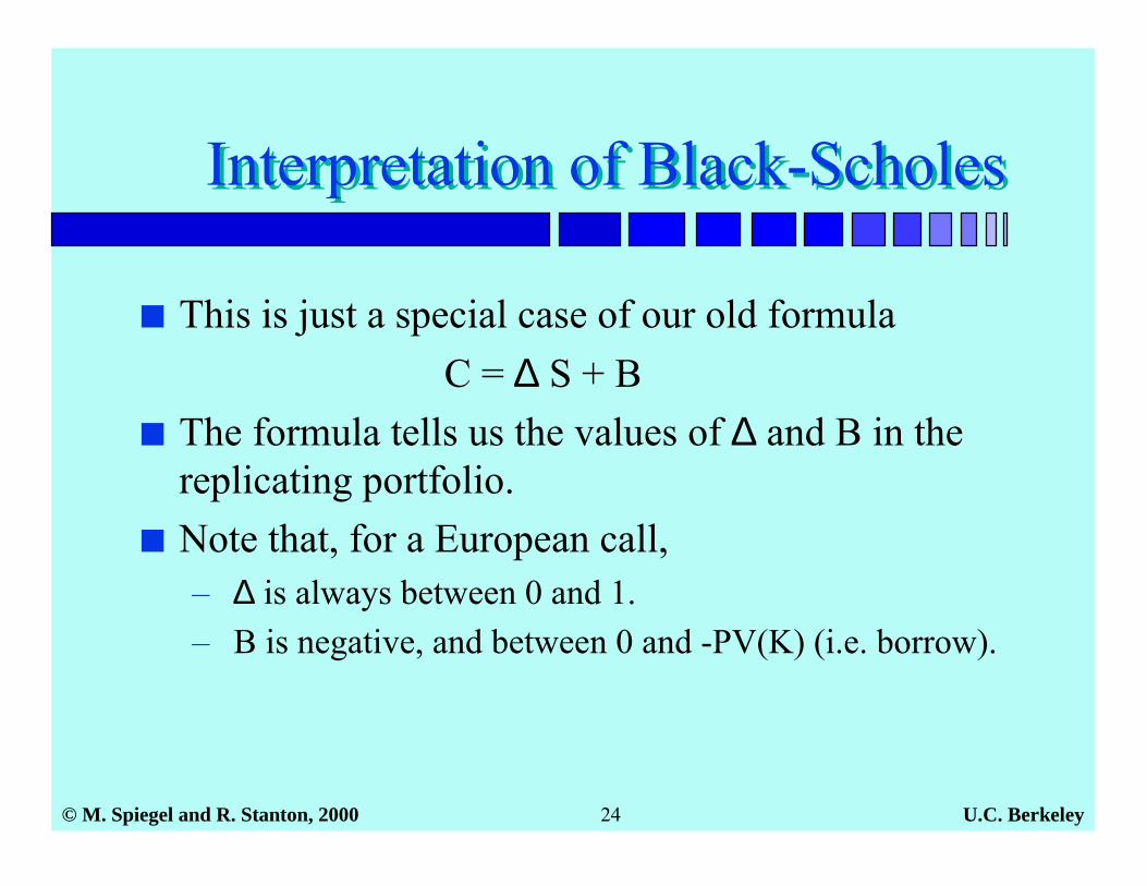
Interpretation of Black-ScholesInterpretation of Black-Scholes

■ This is just a special case of our old formula C = ∆=S + B■ The formula tells us the values of ∆ and B in the

replicating portfolio.■ Note that, for a European call,

– ∆ is always between 0 and 1.– B is negative, and between 0 and -PV(K) (i.e. borrow).


Black-Scholes Call Pricesfor different Maturities

Black-Scholes Call Pricesfor different Maturities

0

5

10

15

20

25

30 35 40 45 50 55 60 65 70

Opt

ion

Valu

e

Stock price

t = 0.0t = 0.1t = 0.5

K = 50r = 0.06σ = 0.3


Black-Scholes put formulaBlack-Scholes put formula

■ Combining the Black-Scholes call result with put-call parity, we obtain the Black-Scholes put value,

■ Note that, for a European put,– ∆ is always between 0 and -1 (i.e. short).– B is positive, and between 0 and PV(K) (i.e. lend).

( )[ ] ( )[ ]( ) ( )[ ]

tσtrKSlogxwhere

,xN1StσxN1KeP

2σ

rt

2++≡

−−−−= −

Options Pricing Lecture 21

Documents

Transcript of Options Pricing Lecture 21