Pricing Options Using Implied Trees: Evidence from FTSE-100 Options

Revised October 2001

Kian-Guan Lim and Da Zhi

* First author is Professor of Finance at the School of Business, the Singapore Management University. Second author is a doctoral

student at the Northwestern University. Computational assistance from Bai Feng and Chang Shiwei, and funding support from the

Institute of High Performance Computing are gratefully acknowledged. The authors also wish to thank the two referees for their

insightful comments that have helped to improve the exposition of this article in significant ways. Correspondence with the first author

at email kglim@smu.edu.sg . Postal address: Prof Lim Kian Guan, School of Business, Singapore Management University, 469 Bukit

Timah Road, Singapore 259756.

Pricing Options Using Implied Trees: Evidence from FTSE-100 Options

Abstract

Previously, few, if any, comparative tests of performance of Jackwerth’s (1997) generalized binomial tree (GBT) and Derman and Kani (1994) implied volatility tree (IVT) models were done. In this paper, we propose five different weight functions in GBT and test them empirically compared to both the Black-Scholes model and IVT.

We use the daily settlement prices of FTSE-100 index options from January to November 1999. With both American and European options traded on the FTSE-100 index, we construct both GBT and IVT from European options and examine their performance in both the hedging of European option and the pricing of its American counterpart. IVT is found to produce least hedging errors and best results for American call options with earlier maturity than the maturity span of the implied trees. GBT appears to produce better results for American ATM put pricing for any maturity, and better in-sample fit for options with maturity equal to the maturity span of the implied trees. Deltas calculated from IVT are consistently lower (higher) than Black-Scholes deltas for both European and American calls (puts) in absolute term. The reverse holds true for GBT deltas. These empirical findings about the relative performance of GBT, IVT, and Standard Black-Scholes models are important to practitioners as they indicate that different methods should be used for different applications, and some cautions should be exercised.

Since the market crash of October 1987, the volatility smile for most world equity markets has become more pronounced. The constant volatility assumption underpinning the Black-Scholes options pricing model (1973)[4] is violated if we assume that the option market is efficient and the options are correctly priced. Tompkins (1998)[35] documents volatility smiles in the UK, Japan, and Germany and compares them with similar smiles in US markets. Studies have extended the Black and Scholes model to account for the volatility smile and other related empirical violations. Jackwerth and Buraschi (1998)[24] group them into two main approaches: Stochastic Volatility models and Deterministic Volatility models.

In Stochastic Volatility models, the evolution of the stock price volatility can be modeled to follow a certain process. Two examples are Brownian motion and mean-

1

reverting process. Hull and White (1987)[19], Ball and Roma (1994)[2], Heston (1993)[18], Stein and Stein (1991)[34], Scott (1987)[31] and Wiggins (1987)[36] study options based on processes with stochastic volatility. These extensions introduce some disadvantages. First, using just the underlying security and risk-free bond is inadequate to hedge the volatility or the jump risk directly, and options valuation is in general no longer preference-free. Second, in these multi-factor models, the option value depends on several additional parameters whose values must be estimated.

Deterministic volatility models are based on the assumption that the local volatility of the underlying asset is a known function of time and of the path and level of the underlying asset price. In these economies, markets are dynamically complete, and options are redundant assets that can be replicated using other assets. Therefore, they can be priced by the no-arbitrage principle without resorting to general equilibrium models, and risk premia do not come into the picture. Moreover, these models can fit the smile exactly by calibrating the local volatility function of the underlying asset. According to Jackwerth and Buraschi (1998)[24] classification, we have (1) the constant elasticity of variance model (Cox and Ross, 1976[7]); (2) the generalized deterministic volatility function models (Dupire, 1994[13] and Derman and Kani, 1994[11]); (3) the implied binomial tree model (Rubinstein, 1994[30]); and (4) the kernel approach (Ait-Sahalia and Lo, 1998[1]).

Implied trees can be applied to models (2) and (3). The basic idea of these approaches is to construct a binomial tree that can fit currently traded derivatives prices whether exactly or in some ways, and the tree can then be used to price any other derivatives on the same underlying asset with the same or earlier maturity. Market implied information embodied in the constructed tree may then help traders’ decision making, and enable the pricing of OTC and exotic options on the same underlying process.

Previously, few, if any empirical tests have been carried out, mainly because of the need for tedious calibration on the generalized binomial tree (GBT) and the implied volatility tree (IVT) models. In this paper, we modify the implied binomial tree model in (3) to a GBT to try to make it better incorporate prices of options that mature within the maturity span of the constructed tree. We test GBT using five different weight functions and compare the performance with the IVT and Black-Scholes model. We calibrate the GBT and IVT using European options with different maturities and test the pricing of American options that are simultaneously traded in the same underlying FTSE-100 index. We empirically compare the pricing performance of these trees and the standard binomial tree (SBT).

There are a few related studies on FTSE-100 index options. In contrast to ours, most of them use parametric approaches by assuming a specific risk-neutral probability distribution and deriving a Black-Scholes-like formula for option pricing. The distribution parameters are then chosen to best fit the observed option prices.

Merfendereski and Rebonato (1999)[28] choose a four-parameter probability distribution, the Generalised Beta of the second kind, and find it is able to fit the observed FTSE-100 index option prices well.

Another recent study on FTSE-100 index option is done by Gemmill and Saflekos (2000)[15]. They estimate the implied distribution, and for the options as a mixture of two lognormals, and find it is better than the one-lognormal approach at fitting observed option prices, and predicting and hedging out-of-sample prices. They also undertake event studies on the shape of the implied distributions during the “crash period”, and

2

find the distribution helps to reveal investor sentiment, but does not have much power for forecasting future events.

In section 1, we briefly review the implied binomial tree (IBT), its extension — generalized binomial tree (GBT), some related techniques to discover the risk-neutral probability distribution, and the implied volatility tree (IVT). Following that, the data are discussed in Section 2. The estimation of optimal weight function is described in Section 3. Section 4 contains both methodology and results of the empirical tests using FTSE-100 options. Finally, Section 5 summarizes the main findings and points out directions for future research.

1 Review of The Implied Tree Models 1.1 Implied Binomial Tree 1.1.1 Obtaining the future probability distribution of the underlying asset Prices of securities contain valuable information that can be used to make a wide variety of economic decisions. In a dynamic equilibrium model with complete markets, the price of any financial security can be expressed as the expected net present value of its future payoffs. The present value is calculated with respect to the riskless rate r and the expectation is taken with respect to the risk-neutral Probability Density Function (PDF) of the payoffs. This PDF, which is distinct from the true PDF of the payoffs, is the risk-neutral PDF or the equivalent martingale measure. More formally, the date-t price of a security with a single liquidating date-T payoff is given by:

tP)( TSZ

TTtTr

Ttr

t dSSfSZeSZEeP )()()]([ ∫−− == ττ

where is a state variable, r is the constant risk free rate of interest between t and TSτ+= tT , and is the date-t risk-neutral PDF for date-T payoffs. )( Tt Sf

Jacques Dreze (1970)[12] recognizes the significant correspondence between state-contingent prices and probability. In the work of Ross (1976)[29], it was found that given a complete set of European option prices on a particular underlying for a particular expiration date, one can deduce the risk-neutral probability distribution (i.e. the PDF) of the underlying for the given expiration date. There are various computational methods to do this, and a good summary of them can be found in Jackwerth (1999)[21].

Longstaff’s method (1990)[26] expresses the probabilities in terms of options prices, strike prices and previous probabilities, and solves for them in a triangular fashion. The result is a set of discrete probabilities following a step function with respect to the strike prices. Rubinstein (1994)[30] discusses the method and finds a few drawbacks: (1) the probabilities frequently vary significantly from very low to very high values over adjoining intervals; (2) negative probabilities can occur; and (3) there are considerable identification problems in the PDF tails.

Shimko (1993)[32] uses Black-Scholes implied volatility as a translation device. Specifically, the method involves the following four steps. (1) Calculate the Black-

3

Scholes implied volatilities for known options (same time to maturity, but different strike price). (2) Fit a smooth curve to the “volatility smile” between the lowest and highest option striking price. (3) Solve for the option prices as a continuous function of the striking price. (4) Take the second derivative of the function. Rubinstein (1994)[30] proposes another method using minimization of fitted price to actual price. Rubinstein’s optimization with prior guess. The implied posterior risk-neutral probabilities, , are the solution to the following quadratic program: jP

∑ −j

jjPPP

j

^2)(min subject to:

∑ =≥=j

jj PP n0,...,jfor 0 and 1

∑=j

njj

N rSPS /)(0 δ

m , ... , 1ifor /]),0max[( =−= ∑ nij

jji rKSPC

Here, is a prior guess of the risk-neutral probabilities; is the nodal underlying asset

price at the end of the tree from the lowest to the highest; is the required ending node

risk-neutral probability, and . Let r and

^

jP jS

jP

∑ =j jP 1 δ represent, respectively, the riskless

interest return and underlying asset payout return over each step. Let be the current price of the underlying asset and be the price simultaneously observed on a European call maturing at the end of the tree with a strike price of . We must choose n > m. The solution can be easily obtained by using software for quadratic optimization with constraints. In Rubinstein’s paper (1994)[30], he starts with a lognormal prior distribution for the terminal stock prices for his study of the S&P 500 index in the period from 1986 to 1993. The lognormal distribution is generated from the Cox-Ross-Rubinstein binomial tree. It is also useful to note that in the above program, the inputs of S

0S

iC

iK

0 and Ci may not be available, but are further constrained to be contained within available bid and ask prices instead. Rubinstein’s optimization with maximum smoothness. The above method requires an assumed prior distribution and occasionally leads to posterior distributions that have sufficiently little smoothness to be plausible. Another interesting approach is to select the implied distribution with maximum smoothness. With all the constraints remaining unchanged, the implied probabilities ’s are chosen to minimize the following function:

jP

∑ +− +−j jjj PPP 2

11 )2( where 010 == +nPP .

Jackwerth and Rubinstein (1996)[22] consider other forms of objective function used for minimization, such as “goodness-of-fit function”, “absolute difference function” and “maximum entropy function”. They find that the implied distributions are rather independent of the choice of the objective function when a sufficiently large number of options are available.

4

1.1.2 Constructing the Implied Binomial Tree After obtaining the risk-neutral probability distribution, the implied binomial tree can then be built. One important assumption of Rubinstein’s original implied binomial tree is that all paths that lead to the same ending node have the same risk-neutral probability. This is often known as the assumption of Binomial Path Independence (BPI). Under BPI, the path probability can be easily obtained by dividing the nodal probability by the number of paths that lead to it. A backward induction technique is then applied to build the entire tree from the ending nodes to the initial node. 1.2 Generalized Binomial Tree One generalization can be made regarding the BPI assumption under the implied binomial tree model. We can assign different probabilities to paths that lead to the same node. Therefore, more information can be incorporated in the tree. For instance, the tree can now be constructed in a way that best fits the prices of any derivatives with expiry before the ending node time, on the same underlying asset. The generalized binomial tree proposed by Jackwerth (1997)[20] accomplishes this by using an optimization method to determine the best linear and generalized weight function that assigns a particular portion of the nodal probability going to the lower preceding node. Such a generalized binomial tree can also incorporate the prices of European options with an earlier maturity. It can also accommodate American options.

Under the implied binomial tree, the number of time steps is indexed by i = 0, 1, . . . , n. The nodes at each step j = 0, 1, . . ., i start with the lowest stock price at the bottom of the step. Then the portion of nodal probability going down to the preceding node is w(j/i) = j/i, and the portion of probability going up is 1 - w(j/i). In other words, the down weight is a linear function of j/i as shown in Figure 1.

Insert “Figure 1: The weight function of implied binomial tree” here

In this way, the entire stock process can effectively be summarized through this weight function together with the ending-node probability distribution. For example, a standard binomial tree can be completely described by a given ending-node probability distribution and a linear weight function. Likewise an implied ending-node risk neutral probability distribution plus a linear weight function summarizes an implied binomial tree.

The tree can then be generalized by changing the weight function. The backward induction of the entire tree can be illustrated using Figure 2.

Here, nodalP , and are nodal probabilities; S, and are the prices of underlying assets; and W(j/i) and W((j – 1)/i) are weights calculated from the weight function.

nodalupP nodal

downP upS downS

Then × × , and transition

probability . Thus, coupled with finding the underlying asset

)/( jiWPnodal =nodalupp W( j/ i) P= ×

nodalupP (1 W(( j 1) / i+ − −

nodalP

)) nodaldownP

/

5

price via risk-neutral expectation using the transition probabilities, working backward on the tree, the entire tree is built. The tree can then be used to price other derivatives that mature earlier or within the maturity span of the implied tree. Each weight function will determine a particular binomial tree, which in turn will determine the prices of other derivatives, and such prices may deviate from the market prices. The purpose is to find an appropriate weight function that, when plugged into the generalized binomial tree model, will be able to price other derivatives accurately.

Insert “Figure 2: One step in Generalized Binomial Tree” here

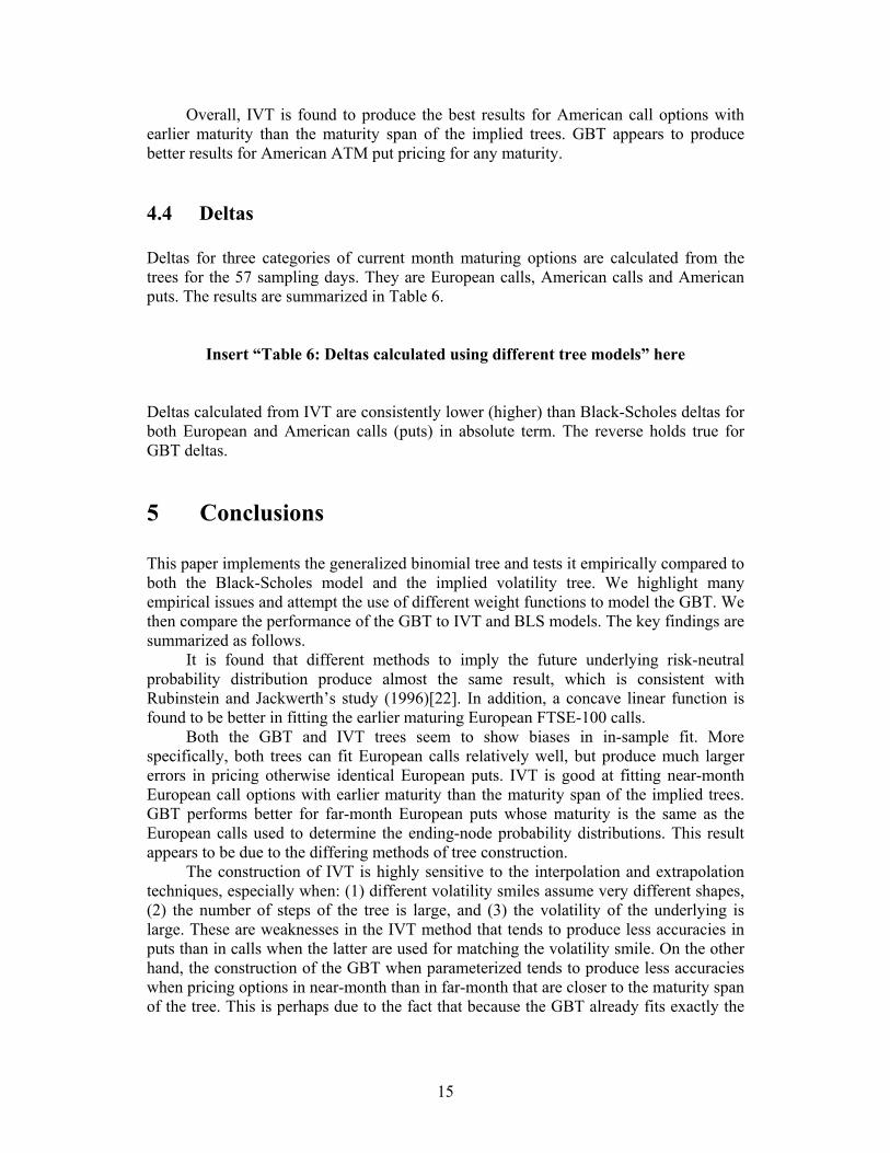
In this paper, we propose five linear and nonlinear weight functions. They share some common characteristics. They pass through (0,0), (1,1). Each function is governed by only one additional parameter, α, that needs to be estimated using optimization method.

Function 1: Linear Concave

1] [0.5, 1] [0.5, Xfor 5.0/)5.0)(1(

0.5] [0, Xfor 5.0/ ∈

∈+−−∈

= ααα

αXX

W

Function 2: Linear Convex Same as Function 1, except that 0.5] ,0[∈α . Function 3: Quadratic Concave

0] [-1, ,)1(2 ∈−+= ααα XXW Function 4: Quadratic Convex Same as Function 3, except 1]. , [0 ∈α Function 5: S curve

2.5] [0, otherwise )10X,0,normcdf(-5

1Xfor 1 0Xfor 0

∈

+==

= αα

W

Function 5 is a cumulative normal distribution function, with mean 0, standard deviation of α . All five functions are plotted in Figure 3.

Insert “Figure 3: Different proposed weight functions” here

6

1.3 Implied Volatility Tree The implied volatility tree model of option pricing was introduced by Derman and Kani of the Quantitative Strategies Group of Goldman Sachs in 1994[10]. It is in spirit similar to the implied binomial tree but different in some ways. The implied binomial tree can only incorporate prices of European options with different strike prices but of the same maturity. GBT extends to the possibility of incorporating options with earlier maturities than the maturity span of the implied tree. The implied volatility tree (IVT), also allows the incorporation of information on European options with different strike prices and different maturities.

In contrast to the GBT’s backward induction, IVT starts from the initial node and expands forward. At any step of the tree, the center node(s) is (are) decided first. Prices and transitional probabilities of all nodes above the center node(s) can be solved in an iterative way by using prices of particular European calls, while prices and transitional probabilities of all nodes below the center node(s) are solved similarly but using prices of particular European puts. These call and put prices are in turn interpolated from the existing market traded options using an implied volatility surface as a transformation tool.

One weakness of IVT is its inability to preclude bad transitional probabilities, which are either greater than 1 or less than 0. In that case, we override the particular nodal price, , that produces the bad probability and set iS 1−×= iii ssS

iS. ( is the

higher node price and is the lower node price in the previous step). If happens to

be at the highest node at that step, i.e.

is

1−is

1+= ni SS , then . If is at lowest

node, i.e. , then . nn Ss /2

iSiS =

1Si S= 221 / Ss=Si

Barle and Cakici (1998)[3] add some improvements to increase the stability of the original Derman and Kani (1994) trees by centering the tree with the forward price. However, arbitrage violations and bad probabilities still occur. Chriss (1996)[6] extends the implied volatility for use with American input options by applying an iterative method, called the false-position method. However, this method is rather computationally involved.

2 Data 2.1 Options FTSE options are traded on The London International Financial Futures Exchange (LIFFE). Both European and American contracts on the same underlying FTSE-100 stock index are traded, which enables a number of interesting studies. For instance, Paul Dawson (1994)[9] has done an empirical analysis of comparative pricing of American and European FTSE-100 Index Options by checking the boundary conditions of early exercise of American options. Not considering transactions costs, some arbitrage possibilities indicate overpriced American options relative to the European options.

7

Both American FTSE-100 index option contracts (SEI) and The European FTSE-100 index option contracts (ESX) expire on the third Friday of the delivery month. A wide range of exercise prices is available for both contracts. However, in order to avoid confusion in the trading pit, exercise prices of American options are offset from the exercise prices of the European contracts by 25 points.

To use both the implied volatility tree model (IVT) and the generalized binomial tree model (GBT), option prices, at one point in time, of a minimum two expiry series, each with different strikes are required. For the convenience of data collection, we choose the “one point of time” as the closing time of the market. We select only the current and subsequent month maturing contracts, that are relatively heavily traded. The prices of European call options are used as the input. In addition, to make Rubinstein’s optimization method and interpolation of volatility smile computationally feasible and meaningful, at least five call option prices for each expiry series are selected.

The data used for this study are primarily from LIFFE. The data comprises a pre-sample set of FTSE-100 European call prices in the period from February to June 1998. This data sample is used to estimate the optimal weight function to employ for the GBT method. The estimation is described in the next section. The sample for the empirical study to compare the performance of the GBT and IVT methods consists of FTSE-100 index option prices in the period from January to November 1999. Data are end-of-day settlement prices. For the empirical studies, in order to ensure independence of the data, we only build trees in odd months, so each tree is built from two months of data. The data for different trees do not overlap. Since maturing contracts expire on the third Friday of that month, only trading days before the third Friday for odd month are included for building each tree. During the sampling period, there are 74 such trading days. However, for 17 days, there are less than 5 call options for each expiry, which leave us with 57 days and in total 2388 options to study.

The underlying index level is provided together with the option data by LIFFE. It is calculated as the average of index values between 4:20pm and 4:30pm (London Time), excluding the eight highest and eight lowest.

The risk-free interest rate used here is the two month LIBOR (London Interbank Borrowing Rate) rate, since the tree is expanding from now till the third Friday of next month. We use the actual index dividend rates. The interest rate and dividend information are obtained from Bloomberg.

3 Estimation of Optimal Weight Function As a first step for GBT, we need to select the optimal ending-node probability distribution fitting method and the weight function. To do this, we use an earlier and separate pre-sample of data so that the empirical results will not be biased.

Three methods are used to obtain the 46-day ending node risk neutral probability distribution at 4:30 pm on February 2, 1998, from the prices of March maturing FTSE-100 stock index Calls. They are Discretized Shimko’s Method (a discretized approximation to the original Shimko’s method as previously described), Rubinstein’s Optimization Method with Prior Guess (the prior guess used here is a lognormal distribution), and Rubinstein’s Optimization Method with Maximum Smoothness.

8

The above three probability distributions are plotted in Figure 4. For the purpose of comparison, we add two more probability distributions. First is the lognormal probability distribution of Black-Scholes model (the curve with highest variance). Second is the probability distribution implied by the calculated IVT for February 2, 1998.

Insert “Figure 4: Future risk-neutral probability distributions implied by different

methods” here

All four implied probability distributions are largely different from the lognormal distribution. Among the four, the IVT implied distribution skews a bit more to the right, which is different from the other three. It is plausible since the IVT may incorporate more information embodied in the current month maturing option contracts in the way the tree is constructed. The other three methods produce roughly the same probability distribution, which reaffirms Rubinstein’s finding that the probability distribution is rather independent of the method used to derive it, given the same input set. Of the three methods, both of Rubinstein’s methods produce somewhat kinky distributions. Shimko’s method produces the smoothest distribution. However, one drawback of this method is that the probabilities are not guaranteed to sum to 1, and consequently may cause trouble when constructing the GBT backwards. For instance, the inferred starting node index level may not exactly equal the current index level. Such a tree will generate large errors when used to price near-maturity options. Due to these considerations, we decide to choose Rubinstein’s method with maximum smoothness to infer the ending-node risk-neutral probabilities, since, by construction, it will produce a smoother distribution. We performed a check on the other sample days till June 1998, and found that this method produces smooth ending-node distributions in most of days.

All five proposed weight functions for constructing the GBT together with the ending-node risk-neutral probability distributions are used to fit European call options data for the first valid trading day for each of the five months from February to June 1998. Since we have more than one call option that matures before the maturity span of the tree, and our proposed functions are all parameterized using α, the earlier calls, unlike the later calls that are used to find the ending-node distribution, are not fitted exactly. For each function, we find the associated α that minimizes Root Mean Square Error (RMSE), with the formula as follows:

∑=

=n

ii neRMSE

1

2 /

The optimal weight )(α , and associated RMSEs of the 5 selected weight functions for current month maturing European Call (C1) and Put (P1) are summarized in Table 1. (Figures are averaged out through five days).

As seen from the table, two convex weight functions (function 2 and 4) collapse to straight lines in all five days, which leads to the same conclusion as in Jackwerth (1997)[20] that concave weight functions are most appropriate. The weight of the quadratic concave function hit the boundary in all 5 days, as the function reaches its maximum skewness at the point where α equals -1. This calls for a concave weight

9

function with higher skewness, and the linear concave function does achieve that with a weight on average of about 0.89. As expected, the linear concave function produces the least RMSE for both C1 and P1 in all months. With the concave weight function, a path looping down first and then coming up is more likely to take place than a path looping up and then coming down.

Insert “Table 1: Different weight functions” here

In summary, for the generalized binomial tree (GBT), we decide to use Rubinstein’s optimization method with maximum smoothness to imply the ending node risk-neutral probability distribution. This probability distribution together with the concave linear weight function will be used to construct the tree. 4 Empirical Tests and Results For the sample data, we categorize 2388 European options (January to November 1999) according to their types and moneyness. The summary statistics are reported in Table 2.

Insert “Table 2: Sample statistics” here

For each of the 57 sampling days, both the generalized binomial tree (GBT) and the implied volatility tree (IVT) are constructed from two sets of European Calls, with one expiring at the current month and the other at the subsequent month.

Both trees have 200 steps, spanning from now to the third Friday of the subsequent month, when the second set expires1.

Since only two sets of options are used as inputs, the interpolation of the volatility surface for IVT is rather simple. For each set, a quadratic curve of the implied volatility as a function of strike price is fitted based on least squares criterion to extract the implied volatility smile. For each strike price, there are two interpolated implied volatilities calculated from the two quadratic curves. These two points are connected with a straight line. We repeat this for all strike prices. The volatility surface will be interpolated in three dimensions like the example in Figure 5.

Insert “Figure 5: The entire volatility surface, February 2 1998” here

For constructing each IVT, interpolation and extrapolation are employed on the

implied volatility curves or smiles. Thus, the call prices that are entered into the solution and construction of the IVT are not the market prices of actual traded calls, but are

2 MATLAB (a mathematical, financial and statistical software language) is used for the programming throughout the study.

10

instead interpolated or extrapolated prices (or more accurately, prices derived from interpolated or extrapolated implied volatilities) of non-existent artificial calls. Since the IVT method requires n/2 number of calls and n/2 number of puts (if n is even), or else (n+1)/2 number of calls and (n-1)/2 number of puts (if n is odd), to compute n+1 nodes for the next forward step, there is a lot more information, but these are generated from the same two sets of input calls.

For constructing each GBT, we could use a linear weight function with more segments and thus more parameters. Indeed, for each day, if there were 5 earlier calls, then using a linear function with 5 segments and thus 5 parameters would fit the call prices exactly. These call prices are actual market call prices, unlike the artificial calls used in the IVT. To be able to provide some form of in-sample comparison between IVT and GBT, our proposed single-parameter weight function allows for in-sample non-trivial errors in the GBT method while employing the same two sets of input calls as in the IVT.

This should not be construed as biasing the performance test against the GBT in favor of IVT. There are two reasons. From a practical point of view, when there are numerous traded options, it becomes computationally intractable to customize many linear segments of the weight function in order to provide an exact fit. It should also be noted that depending on the sequence of options, the piecewise linear function is not necessarily unique. This leads to the notion of selecting an optimal function. An approach would be to relax the fit and be able to parameterize the function. This notion is consistent with what we do in this paper. Secondly, one should not forget that the GBT already fits exactly the call prices with maturity at the ending-nodes. This may also be construed as an unfair advantage of GBT over the IVT since the latter does not provide for an exact fit. Rather, the holistic theme of the comparison in GBT and IVT is to study how forward propagation of the tree by IVT versus backward propagation by GBT, and the different ways in which the identifying restrictions are set up in estimating the nodal security values and transitional probabilities affect the pricing of other options, including American, not used to calibrate the trees. 4.1 In-sample test In the in-sample test, the abilities of the GBT and IVT to explain the prices of European calls and puts within the maturity span of the trees are compared. Thus, apart from the calls used as inputs to build the two trees, the trees are also used to price other European puts that mature in both months. RMSEs are calculated each day for four categories of options: current-month maturing European calls (puts) and subsequent month maturing European calls (puts). The results are shown in Table 3.

Insert “Table 3: In-sample fit performance of two implied trees” here GBT is bound to price C2 exactly as it is one of the constraints in Rubinstein’s

optimization method used to imply the ending-node risk-neutral probability distribution. The advantage of exact fitting of the C2 calls in GBT also helps in better in-sample performance of P2 put pricing for GBT compared to IVT. However, the fitting of

11

current-month maturing options for GBT is not as good as IVT. This on the other hand is perhaps due to the better employment of information based on implied volatility fit of C1 (earlier) call options under IVT. This better employment may be a result of the flexibility of IVT in using such earlier option price information through its implied volatility fitting. It is perhaps more flexible and efficient in incorporating earlier option price information than GBT does when partial and not full parameterization is used in its backward propagation of the tree.

On the other hand, the IVT also has weaknesses. The IVT starts from the first node, and nodal prices at a higher level will incorporate those prices at a lower level and previous steps. There may be errors introduced in the tree for two reasons. First, the interpolation and extrapolation techniques are too simple to capture the real market implied volatility surface. Second, the arbitrary centering condition applied when encountering bad probabilities may also introduce error. Such errors will be accumulated as the tree expands forward, which results in larger errors in pricing subsequent month maturing options. IVT is found to be extremely sensitive to the interpolation technique when the smiles are of very different shapes, when the step of the tree is large and when the volatility of the underlying is very high.

The trees are constructed using European Calls only. We find that the error is much larger when the trees are used to price European puts than when used to price other European calls, specifically P1 for GBT and P2 for IVT. The typical bid-ask spread of the FTSE-100 index Option in LIFFE ranges from 6 to 11. We find most RMSEs of the fitting errors are within the bid-ask spread.

Many researchers have done empirical tests on put-call parity (PCP), among others, Gould and Galai (1974)[16], Klemkosky and Resnick (1979)[25], (1980), Evnine and Rudd (1985)[14], Chance (1987)[5], Loudon (1988)[27] and Gray (1989)[17]. Their conclusions can be best summarized by noting that while PCP holds, on average, there are frequent, substantial violations of PCP involving both overpricing and underpricing of calls and puts. In our context, the difference in the put pricing from call pricing is not related to the PCP issue or observations, as the larger deviations are mostly within the bid-ask spreads. If we also account for transaction costs, then it is generally agreed that PCP is not an issue, even elsewhere.

There could be other reasons for the larger put pricing deviations. First, we use the current dividend rate and assume it is the same throughout the tree. Second, the volatility implied from European calls in practice may differ from that implied from puts. The IVT will be more sensitive to the latter implication.

4.2 Simple Delta Hedge of Current-month Maturing European Call Options

Here we will compare the hedging performance of IVT and GBT against Black-Scholes in a simple delta hedge.

At the end of each trading day before the maturity date of that month, three current month maturing European calls nearest to ATM strike are chosen. Deltas or will be calculated for the three chosen calls. Three portfolios are then constructed, each by longing one call and shorting respective

s∆

∆ units of FTSE-100 index portfolio. The portfolios are liquidated at the end of the next trading day, and new portfolios are then constructed. The hedging errors are calculated as follows:

12

)()( 11 iiATMi

ATMi

ATMi

ATMi FTSEFTSECCe −∆−−= ++

)()( 11 iiITMi

ITMi

ITMi

ITMi FTSEFTSECCe −∆−−= ++

)()( 11 iiOTMi

OTMi

OTMi

OTMi FTSEFTSECCe −∆−−= ++

OTMi

ATMi

ITMi

totali eeee ++=

Hedging errors in all four categories for all three models are computed for analyses. The means and standard deviations of these errors across time are reported in Table 4.

Insert “Table 4: Simple delta-hedging performance” here

We find that both BLS and IVT produce negative hedging errors. IVT produces

the smallest hedging errors and the standard deviations of the errors are comparable with those of BLS.

GBT does not show any biases in mean hedging error. However, it demonstrates much larger standard deviations, which is mainly a result of its much larger deltas.

4.3 Pricing of the current month maturing American option Assuming the European FTSE-100 index option market is efficient, information extracted from the prices of such European options must reflect the true market valuation of risk and return, given their expectation of future movements of the index. If such information is used to price the American counterparts, superior results will be expected.

Here, IVT and GBT are compared against the standard binomial tree with constant volatility in the pricing of American options. The standard binomial tree constructed here consists of 200 steps. In a SBT, the up and down move at each step are governed by the volatility of the underlying index as follows: 200/teσ=u and 200/teu σ−= , where σ is the annualized standard deviation of the underlying index and t is the time to maturity. For a particular American option, the σ used is the Black-Scholes implied volatility of an otherwise identical European option, which is in turn interpolated or extrapolated from the smile using the previously described quadratic function.

For the American options, we follow a similar procedure as in the hedging of European call options. For the end of each trading day before the maturity date of that month, we choose three current month maturing American calls and puts nearest to ATM strike price. We calculate the model prices using three trees, with the possibility of early exercise being checked at each node in the tree. The model prices are those compared with the market closing price. Both Average Percentage Pricing Error (APPE) and RMSE are computed. The formula for APPE is as follows:

%100×−

=P

PPAPPE m

13

where P is the market price and is the model price. APPE’s across time will be compared with 0 to detect any possible pattern of over-pricing or under-pricing. The results are summarized in table 5.

mP

Insert “Table 5: Pricing of current month maturing American Options” here

Overall, IVT outperforms the other two in terms of smaller Root Mean Square Errors for each of the six months and for all categories of American calls and nearly all of American puts. Both IVT and GBT price the current-month maturing calls more accurately in terms of average percentage pricing error than standard binomial tree (SBT), which assumes constant volatility. There appears to be under-pricing for both SBT and IVT in all three categories of American calls. However, the average percentage pricing error for calls is negative for GBT, which indicates overpricing.

IVT seems to be more accurate in the pricing of American call options. Since IVT is constructed from the European calls and is able to price the current-month maturing European call well, then the existence of consistent underpricing of the current month maturing American calls may have two explanations. (1) IVT does not adequately capture the entire early exercise premium. This could be due to a so-called “wild card” option. The daily settlement price is based on the average level of the FTSE 100 Index between 4:20pm and 4:30pm (London time), but the exercise can be delayed to 4:45pm. During the period from 4:30pm to 4:45pm, the arrival of price sensitive information does not affect the cash settlement available to the holders of FSTE-100 American options who choose to exercise that day, but does influence the opening value of such options if they are held till the following business day. This feature can be considered as a put option on the American index option itself. It proves to be an important factor in the pricing of short-term American options. However, all three models fail to account for this feature, which may lead to underpricing. (2) The American call options are overpriced relative to the European counterparts. IVT, which fits ITM European calls well, performs not as well for the American counterparts. However, with all options’ time to maturity less than 20 days, such errors seem too large to be explained by the inability of IVT to capture the entire early exercise premium or even the “wild card” option as described above.

The pricing of the American put option produces less accurate results than that of the American call. One reason is that the early exercise premium of American puts is greater than for similar calls, as shown in Zivney’s empirical study (1991)[37]. Put options can have rational early exercise even if there is no payout from the underlying. Another reason is that the information for constructing the tree is extracted from only call options. As the in-sample test shows, calls and puts do not appear to contain exactly identical information. The results are mixed. No model seems to dominate in both criteria: mean percentage mispricing error and RMSE for all categories. For ATM American puts, SBT gives the smallest APPE and GBT gives the smallest RMSE. For OTM American puts, SBT again gives the smallest APPE but IVT gives the smallest RMSE. As for the moneyness bias, GBT and IVT appear to consistently under-price the American puts while SBT does not appear to carry this bias for ITM puts.

14

Overall, IVT is found to produce the best results for American call options with earlier maturity than the maturity span of the implied trees. GBT appears to produce better results for American ATM put pricing for any maturity.

4.4 Deltas Deltas for three categories of current month maturing options are calculated from the trees for the 57 sampling days. They are European calls, American calls and American puts. The results are summarized in Table 6.

Insert “Table 6: Deltas calculated using different tree models” here Deltas calculated from IVT are consistently lower (higher) than Black-Scholes deltas for both European and American calls (puts) in absolute term. The reverse holds true for GBT deltas. 5 Conclusions This paper implements the generalized binomial tree and tests it empirically compared to both the Black-Scholes model and the implied volatility tree. We highlight many empirical issues and attempt the use of different weight functions to model the GBT. We then compare the performance of the GBT to IVT and BLS models. The key findings are summarized as follows.

It is found that different methods to imply the future underlying risk-neutral probability distribution produce almost the same result, which is consistent with Rubinstein and Jackwerth’s study (1996)[22]. In addition, a concave linear function is found to be better in fitting the earlier maturing European FTSE-100 calls.

Both the GBT and IVT trees seem to show biases in in-sample fit. More specifically, both trees can fit European calls relatively well, but produce much larger errors in pricing otherwise identical European puts. IVT is good at fitting near-month European call options with earlier maturity than the maturity span of the implied trees. GBT performs better for far-month European puts whose maturity is the same as the European calls used to determine the ending-node probability distributions. This result appears to be due to the differing methods of tree construction.

The construction of IVT is highly sensitive to the interpolation and extrapolation techniques, especially when: (1) different volatility smiles assume very different shapes, (2) the number of steps of the tree is large, and (3) the volatility of the underlying is large. These are weaknesses in the IVT method that tends to produce less accuracies in puts than in calls when the latter are used for matching the volatility smile. On the other hand, the construction of the GBT when parameterized tends to produce less accuracies when pricing options in near-month than in far-month that are closer to the maturity span of the tree. This is perhaps due to the fact that because the GBT already fits exactly the

15

call prices with maturity at the ending-nodes, pricing of options nearer to the end produces superior results.

Compared to the Black-Scholes model, IVT consistently produces smaller deltas for both European and American calls, while GBT’s deltas are much larger due to its highly skewed weight function. The results for both European and American puts (in absolute term) are reversed.

In hedging near-month European calls using the simplest delta hedge, IVT gives the smallest hedging error. Both IVT and Black-Scholes model consistently show negative total hedging errors. This seems to call for more sophisticated hedging strategies and perhaps more than one instrument to hedge higher order risks.

IVT and GBT are constructed using European call options. When they are used to price the American counterparts, IVT is found to outperform both SBT and GBT in pricing the American calls with earlier maturity than the maturity span of the implied trees. GBT appears to produce better results for American ATM put pricing for any maturity. The methods appear to produce under-pricing of the American options.

Jackwerth and Rubinstein (2001)[23] undertake a preliminary study of S&P index options by comparing a large variety of models in explaining otherwise identical observed option prices, but with different strike prices, or with different times-to-expiration, or at different points in time. They find traders’ naive predictive models perform best in out-of-sample forecast. An interesting extension is to employ GBT and IVT trees for out-of-sample forecasting. Since forecasting issues need a whole different set of assumptions and diverge from the in-sample comparisons and calibrations for American option done in this paper, this should be done as a separate study.

The implied tree model can also be compared with other deterministic volatility models, such as the more traditional CEV model of Cox and Ross(1976)[7], and the more recent kernel model of Ait-Sahalia and Lo (1998)[1]. Besides, they can also be tested against other trees with stochastic volatility.

This paper has performed some interesting empirical comparisons of the relative performance of GBT, IVT, and Standard Black-Scholes models. The holistic theme of the comparison in GBT and IVT is to study how forward propagation of the tree by IVT versus backward propagation by GBT, and the different ways in which the identifying restrictions are set up in estimating the nodal security values and transitional probabilities affect the pricing of other derivatives based on the same trees.

The results are important to practitioners as they indicate that different methods should be used for different applications, and some cautions should be exercised.

References [1] Yacine Ait-Sahalia and A. W. Lo. Non-Parametric Estimation of State-Price Densities

Implicit in Financial Asset Prices. Journal of Finance, 53(2): 499–547, 1998. [2] C. Ball and A. Roma. Stochastic Volatility Option Pricing. Journal of Financial and

Quantitative Analysis, 29(4): 589–607, 1994. [3] S. Barle and N. Cakici. How to Grow a Smiling Tree. Journal of Financial Engineering, 7(2):

127–146, 1998. [4] F. Black and M. Scholes. The Pricing of Options and Corporate Liabilities. Journal of

Political Economy, 81: 637–657, 1973.

16

[5] D.M. Chance. Parity Test of Index Options. Advances in Futures and options Research, 2:47–64, 1987.

[6] N. Chriss. Transatlantic Trees. RISK, 7, 1996. [7] J. Cox and S. Ross. The Valuation of Options for Alternative Stochastic Processes. Journal of

Financial Economics, January-March: 145–166, 1976. [8] J. Cox, S. Ross, and M. Rubinstein. Option Pricing: A Simplified Approach. Journal of

Financial Economics, (7): 229–263, 1979. [9] P. Dawson. Comparative Pricing of American and European Index Options: An Empirical

Analysis. Journal of Futures Markets, 14(3): 363–378, 1994. [10] Derman E., and I. Kani. The Volatility Smiles and Its Implied Tree. Goldman Sachs

Quantitative Strategies Research Notes, January 1994. [11] Derman E., and I. Kani. Riding on a Smile. RISK, 7(2), 32–39, 1994. [12] Jacques. Dreze. Market Allocation Under Uncertainty. European Economic Review, 2:133–

165, 1970. [13] B. Dupire. Pricing with a Smile. RISK, 7(1), 18–20, 1994. [14] J. Evnine and A. Rudd. Index Options: The Early Evidence. Journal of Finance, 40:743–

755, 1985. [15] G. Gemmill and A. Saflekos. How Useful Are Implied Distributions? Evidence from Stock

Index Options. Journal of Derivatives, spring: 83–98, 2000. [16] J.P. Gould and D. Galai. Transaction Costs and the Relationship between Put and Call

Prices. Journal of financial Economic, July: 105–129, 1974. [17] S.F. Gray. Put Call Parity: An Extension of Boundary Conditions. Australian Journal of

Management, 14(2): 151–169, 1989. [18] S. Heston. A Closed-Form Solution for Options with Stochastic Volatility with Applications

to Bond and Currency Options. Review of Financial Studies, X (6): 326–343, 1993. [19] J. Hull and A. White. The Pricing of Options on Assets with Stochastic Volatility. Journal

of Finance, 42(2): 281–300, 1987. [20] J. C. Jackwerth. Generalized Binomial Trees. Journal of Derivatives, 5, No. 2, 7–17, 1997. [21] J. C. Jackwerth. Implied Binomial Trees: A Literature Review. Journal of Derivatives 7, No.

2, 66–82, 1999. [22] J. C. Jackwerth and M. Rubinstein. Recovering Probability Distributions from Options

Prices. Journal of Finance, 51(5): 1611–1631, 1996. [23] J. C. Jackwerth and M. Rubinstein. Recovering Stochastic Processes from Option Prices.

Abstract in Journal of Finance 52(3): 1236, 2001. [24] J.C. Jackwerth and A. Buraschi. Explaining Option Prices: Deterministic vs. Stochastic

Models. Working Paper, 1998. [25] R.C. Klemkosky and B.G. Resnick. Put-Call Parity and Market Efficiency. Journal of

Finance, 34:1141–1155, 1979. [26] Francis Longstaff. Martingale Restriction Tests of Option Pricing Models. Working paper,

1990, UCLA. [27] G. Loudon. Put Call Parity Theory: Evidence from the Big Australian. Australian Journal of

Management, 13:53–59, 1988. [28] D. Mirfendereski and R. Rebonato. Closed-Form Solutions for Option Pricing in the

Presence of Volatility Smiles: A Density-Function Approach. The Journal of Risk, 3, 2001. [29] Stephen. Ross. Options and Efficiency. Quarterly Journal of Economics, 90:75–89, 1976. [30] M. Rubinstein. Implied Binomial Trees. Journal of Finance, 69(3): 771–818, 1994. [31] L.O. Scott. Option Pricing when the Variance Changes Randomly: Theory, Estimation and

an Application. Journal of Financial and Quantitative Analysis, 22:419–438, 1987. [32] D. Shimko. Bounds of Probability. RISK, (4): 33–37, 1993. [33] Hodges S. Skiadopoulos, G. and L. Clewlow. The Dynamics of the S&P 500 Implied

Volatility Surface. Working paper, 1999. [34] E. Stein and C. Stein. Stock Price Distributions for Estimating Stochastic Volatility: An

Analytic Approach. Review of Financial Studies, (4): 727–752, 1993.

17

[35] Robert G. Tompkins. Implied Volatility Surfaces: Uncovering Regularities for Options on Financial Futures. Working paper, Vienna University of Technology, 1998.

[36] J. Wiggins. Option Values Under Stochastic Volatility. Journal of financial Economics, 19(2): 351–372, 1987.

[37] T.L. Zivney. The Value of Early Exercise in Option Prices: An Empirical Investigation. Journal of Financial and Quantitative Analysis, 26(1): 129–138, 1991.

18

Figure 1: The weight function of implied binomial tree

19

Figure 2: One step in Generalized Binomial Tree

20

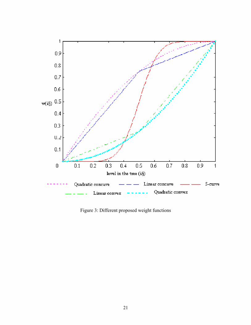
Figure 3: Different proposed weight functions

21

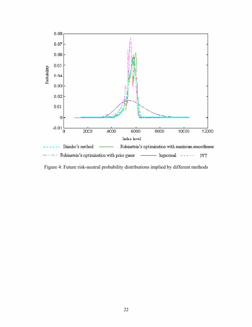
Figure 4: Future risk-neutral probability distributions implied by different methods

22

Figure 5: The entire volatility surface, February 2 1998

23

Table 1: Different weight functions

We test five different weight functions and calculate the optimal weight, RMSE (root mean square error) of current-month maturing European calls (C1) and puts (P1) for each function. The figures are averaged out across the various months.

Weight Functions Weight ( )α RMSE of C1 RMSE of P1

Linear Concave 0.89 5.32674 5.18974

Linear Convex 0.5 20.71164 18.86668

Quadratic Concave -1 17.00998 15.78394

Quadratic Convex 0 20.71164 18.86668

S-curve function 1.96 13.47964 19.5748

Notes: The five different proposed weight functions pass through (0,0), (1,1). Each function is governed by parameter α as follows. (1) Linear Concave:

1] [0.5, 1] [0.5, Xfor 5.0/)5.0)(1(

0.5] [0, Xfor 5.0/ ∈

∈+−−∈

= ααα

αXX

W

(2) Linear Convex: Same as Function 1, except that 0.5] ,0[∈α .

(3) Quadratic Concave: W . 0] [-1, ,)1(2 ∈−+= ααα XX(4) Quadratic Convex: Same as Function 3, except 1]. , [0 ∈α

α(5) S curve: cdf has mean 0 and standard deviation of .

2.5] [0, otherwise )10X,0,normcdf(-5

1Xfor 1 0Xfor 0

∈

+==

= αα

W

24

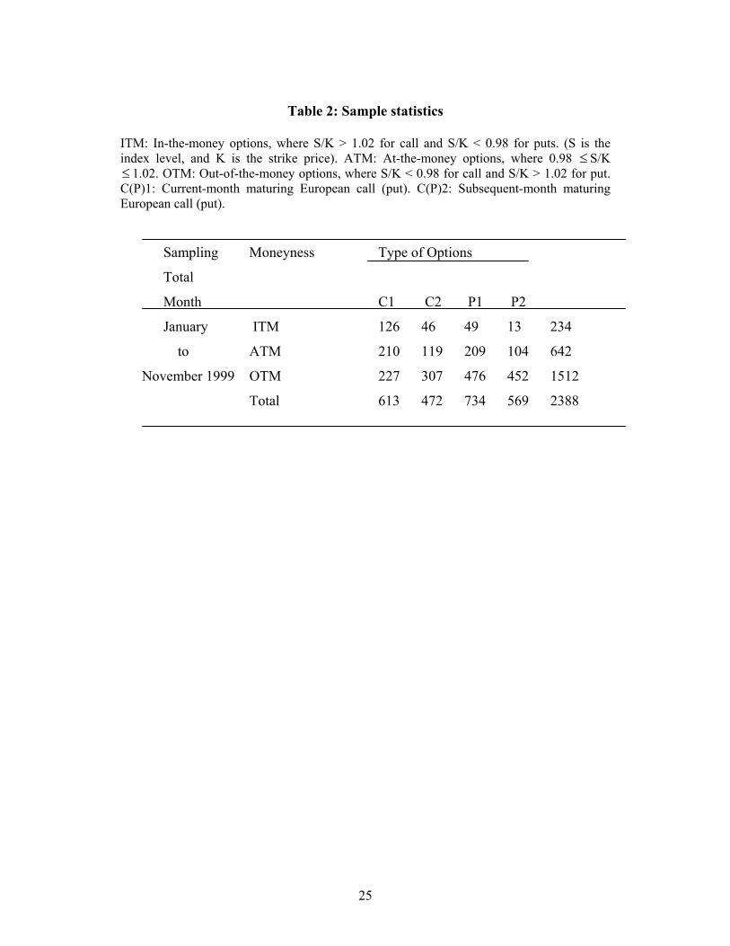
Table 2: Sample statistics

ITM: In-the-money options, where S/K > 1.02 for call and S/K < 0.98 for puts. (S is the index level, and K is the strike price). ATM: At-the-money options, where 0.98 ≤S/K

1.02. OTM: Out-of-the-money options, where S/K < 0.98 for call and S/K > 1.02 for put. C(P)1: Current-month maturing European call (put). C(P)2: Subsequent-month maturing European call (put).

≤

Sampling Moneyness Type of Options

Total

Month C1 C2 P1 P2

January ITM 126 46 49 13 234

to ATM 210 119 209 104 642

November 1999 OTM 227 307 476 452 1512

Total 613 472 734 569 2388

25

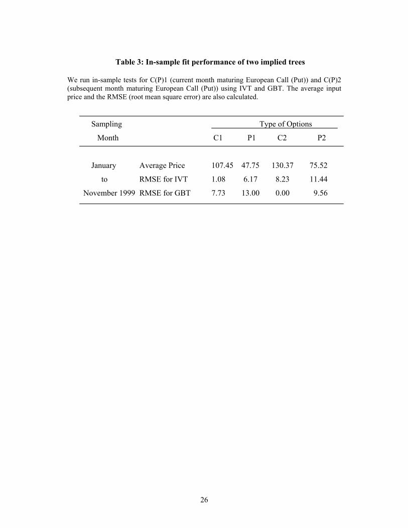
Table 3: In-sample fit performance of two implied trees

We run in-sample tests for C(P)1 (current month maturing European Call (Put)) and C(P)2 (subsequent month maturing European Call (Put)) using IVT and GBT. The average input price and the RMSE (root mean square error) are also calculated.

Sampling Type of Options

Month C1 P1 C2 P2

January Average Price 107.45 47.75 130.37 75.52

to RMSE for IVT 1.08 6.17 8.23 11.44

November 1999 RMSE for GBT 7.73 13.00 0.00 9.56

26

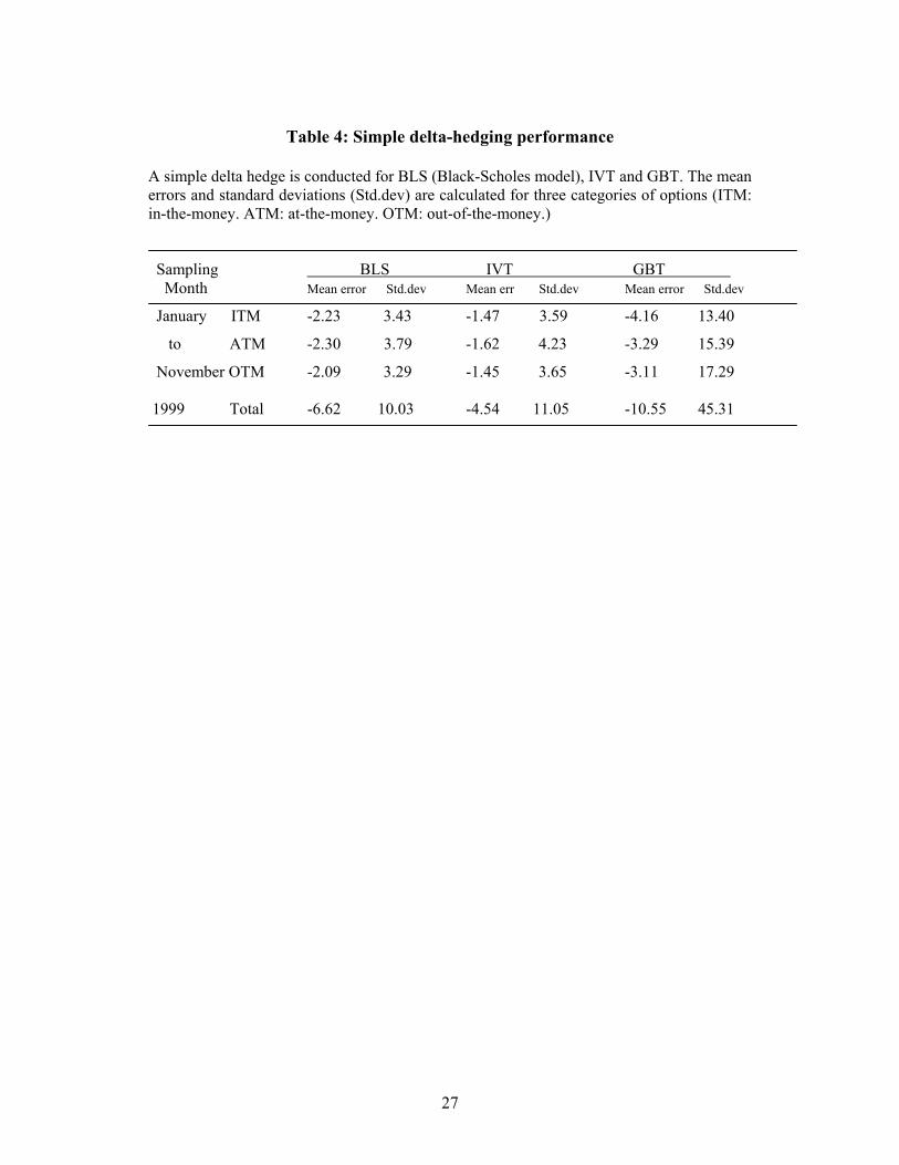
Table 4: Simple delta-hedging performance

A simple delta hedge is conducted for BLS (Black-Scholes model), IVT and GBT. The mean errors and standard deviations (Std.dev) are calculated for three categories of options (ITM: in-the-money. ATM: at-the-money. OTM: out-of-the-money.) Sampling BLS IVT GBT Month Mean error Std.dev Mean err Std.dev Mean error Std.dev

January ITM -2.23 3.43 -1.47 3.59 -4.16 13.40

to ATM -2.30 3.79 -1.62 4.23 -3.29 15.39

November OTM -2.09 3.29 -1.45 3.65 -3.11 17.29 1999 Total -6.62 10.03 -4.54 11.05 -10.55 45.31

27

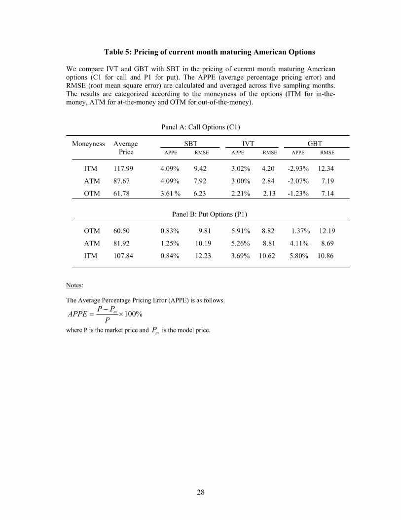
Table 5: Pricing of current month maturing American Options We compare IVT and GBT with SBT in the pricing of current month maturing American options (C1 for call and P1 for put). The APPE (average percentage pricing error) and RMSE (root mean square error) are calculated and averaged across five sampling months. The results are categorized according to the moneyness of the options (ITM for in-the-money, ATM for at-the-money and OTM for out-of-the-money).

Panel A: Call Options (C1)

Moneyness Average SBT IVT GBT Price APPE RMSE APPE RMSE APPE RMSE

ITM 117.99 4.09% 9.42 3.02% 4.20 -2.93% 12.34

ATM 87.67 4.09% 7.92 3.00% 2.84 -2.07% 7.19

OTM 61.78 3.61 % 6.23 2.21% 2.13 -1.23% 7.14

Panel B: Put Options (P1)

OTM 60.50 0.83% 9.81 5.91% 8.82 1.37% 12.19

ATM 81.92 1.25% 10.19 5.26% 8.81 4.11% 8.69

ITM 107.84 0.84% 12.23 3.69% 10.62 5.80% 10.86

Notes: The Average Percentage Pricing Error (APPE) is as follows.

%100×−

=P

PPAPPE m

where P is the market price and is the model price. mP

28

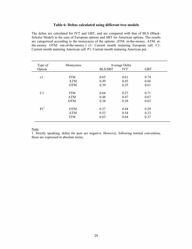
Table 6: Deltas calculated using different tree models

The deltas are calculated for IVT and GBT, and are compared with that of BLS (Black-Scholes Model) in the case of European options and SBT for American options. The results are categorized according to the moneyness of the options. (ITM: in-the-money. ATM: at-the-money. OTM: out-of-the-money.) c1: Current month maturing European call. C1: Current month maturing American call. P1: Current month maturing American put.

Type of Moneyness Average Delta Option BLS/SBT IVT GBT c1 ITM 0.65 0.61 0.74

ATM 0.49 0.45 0.66 OTM 0.39 0.35 0.61

C1 ITM 0.64 0.57 0.71

ATM 0.48 0.47 0.67 OTM 0.38 0.38 0.63

P11 OTM 0.37 0.44 0.29

ATM 0.53 0.54 0.33 ITM 0.63 0.64 0.37

Note: 1. Strictly speaking, deltas for puts are negative. However, following normal convention, these are expressed in absolute terms.

29