Optimum Representation of the Blade Shape

and the Design Variables in Inverse Blade Design

Shayesteh Mohammadbeigy

A Thesis

in

The Department

of

Mechanical and Industrial Engineering

Presented in Partial Fulfillment of the Requirements

For the Degree of Master of Applied Science (Mechanical Engineering) at

Concordia University

Montreal, Quebec, Canada

April 2016

© Shayesteh Mohammadbeigy, 2016

Concordia University

School of Graduate Studies

This is to certify that the thesis prepared

By: Shayesteh Mohammadbeigy

Entitled: Optimum Representation of the Blade Shape and the Design Variables in Inverse

Blade Design

and submitted in Partial Fulfillment of the Requirements for the Degree of

Master of Applied Science (Mechanical)

Complies with the regulation of the University and meets the accepted standards with respect to

originality and quality.

Signed by the final Examining Committee:

_____________________________ Chair

_____________________________ Examiner

_____________________________ Examiner

_____________________________ Supervisor

Approved by: _________________________________________________

_________________________________________________

Date _________________________________________________

Dr. Wahid Ghaly

Dr. Samuel Li

Dr. Marius Paraschivoiu

Dr. Hoi Dick Ng

Chair of Department or Graduate Program Director

Dean of Faculty

iii

ABSTRACT

Optimum Representation of the Blade Shape and the Design Variables in Inverse Blade Design

Shayesteh Mohammadbeigy

A flexible yet precise method for prescribing and modifying the blade shape and the inverse design

variables in two- (2D) and three-dimensional (3D) flow is presented. It is based on B-spline functions to

represent curves (in 2D) and surfaces (in 3D) and enables one to approximate an existing blade shape or to

specify target pressure distributions (or pressure loading). The notable characteristics of B-splines

including smoothness, flexibility and robustness have made them well-suited to accurately fit

both the design variables and the geometry.

The precision and stability of B-splines in representing the airfoil geometry has been

illustrated by interpolating generic and actual 2D airfoils. Care has been taken to enhance the

representation especially in high curvature areas, e.g. LE and TE, by the proper choice of B-

spline parameters. B-spline surface generation has been integrated in the extension of the present

2D inverse design into a fully three-dimensional inverse shape design.

On the other hand, a method based on B-splines has been developed for generating the

target pressure and loading distributions in both streamwise and spanwise directions. The method

provides the designer with sufficient local control on the target profile, it is easy to use in

generating smooth target pressure (or loading) curves and surfaces using a few input parameters

from the designer.

The developed technique is used to generate target pressure distributions or loading distribution for

redesigning a highly loaded transonic turbine vane, and the rotor of a subsonic compressor stage under

iv

different operating conditions using a previously developed 2D inverse shape design method that is

implemented into ANSYS-CFX where the unsteady Reynolds-Averaged Navier-Stokes

equations are solved and the 𝑘 − 𝜔 turbulence model is used for all test cases. The airfoils

performance has been improved as a result of the target design variables meticulously tailored to

satisfy all the design intents.

v

ACKNOWLEDGEMENT

I would like to thank all the people who have helped me during the course of this research.

I would like to express my sincere gratitude to my supervisor, Dr. Wahid Ghaly, for his

guidance, motivation, inspiration and continuous support during the course of this work.

Special thanks go to my colleague and friend, Araz Arbabi for his support, help and

advice. I will not forget the unnumbered lab discussions we had and the solutions and ideas we

came up with together.

Last but not least, I would like to express my deepest appreciation to my wonderful

parents for their support, empathy and all the motivation and courage they have given me in

pursuing my dreams throughout my life.

vi

TABLE OF CONTENTS

List of Figures viii

List of Tables xi

List of Symbols xii

1 Introduction 1

1.1 Previous Investigations ............................................................................................... 2

1.2 Present Investigations .................................................................................................. 5

1.3 Thesis Outline ............................................................................................................. 7

2 Governing Equations and Methodology 8

2.1 Flow Governing Equations.......................................................................................... 8

2.1.1 User Defined Function ................................................................................... 12

2.1.2 Mesh Motion .................................................................................................. 12

2.1.3 Mesh Stiffness ................................................................................................ 14

2.1.4 Mesh Considerations ...................................................................................... 15

2.2 Inverse Design Methodology .................................................................................... 17

2.2.1 Inverse Design Formulation ........................................................................... 18

2.2.2 Design Variables ............................................................................................ 21

2.2.3 Design Considerations .................................................................................... 23

3 Airfoil Shape and Design Variables Representation and Modification 24

3.1 Representation of 2D Airfoils with B-Splines .......................................................... 26

3.1.1 Generic Blade ................................................................................................. 27

3.1.2 E/CO-1 Compressor Blade ............................................................................. 29

3.1.3 Rotor 67 .......................................................................................................... 30

3.1.4 Effect of Number of Control Points on the Error ........................................... 30

3.1.5 Effect of Control Points Clustering on the Error ............................................ 31

3.1.6 Effect of Curve Degree on the Error .............................................................. 33

3.2 Tailoring the Target Pressure Distribution Using B-Splines .................................... 34

3.2.1 Roidl’s Method ............................................................................................... 35

3.2.2 Graphical User Interface ................................................................................ 39

4 Inverse Design Algorithm and Redesign Results 42

vii

4.1 VKI-LS89 Turbine Vane Redesign ........................................................................... 45

4.1.1 Redesigning VKI-LS89 in Subsonic Outflow Condition ............................... 48

4.1.2 Redesigning VKI-LS89 in Transonic Outflow Condition ............................. 52

4.2 E/CO-3 Compressor Stage Redesign ........................................................................ 56

4.2.1 Redesigning E/CO-3 at Maximum Flow Condition ....................................... 58

4.2.2 Redesigning E/CO-3 at Near Surge Condition ............................................... 62

4.2.3 E/CO-3 Compressor Stage Redesign Performance Gain over the Previous

Method ............................................................................................................ 65

5 Conclusion 68

5.1 Summary ................................................................................................................... 68

5.2 Future Work .............................................................................................................. 69

References 71

A B-Spline Curve and Surface Interpolation 74

A.1 B-Spline Preliminaries .............................................................................................. 75

A.2 B-spline Surface Interpolation .................................................................................. 78

B The Pressure GUI 83

B.1 Target Loading Curve Generation............................................................................. 89

B.2 Target Loading Surface Generation .......................................................................... 91

viii

LIST OF FIGURES

Figure 2.1: Mesh close-up near the LE and TE of VKI-LS89 ................................................. 16

Figure 2.2: Blade wall movement (reprinted from [27]) ......................................................... 20

Figure 3.1: Generic compressor profile; 25 Control points, 2nd degree ................................... 28

Figure 3.2: Generic Blade and 2nd degree B-splines fitted to control points with different

distributions.............................................................................................................................. 32

Figure 3.3: Generic blade fitted with evenly and unevenly distributed points at the TE ........ 32

Figure 3.4: Generic blade fitted with evenly and unevenly distributed points at the LE ........ 32

Figure 3.5: E/CO-1 interpolated by quadratic and cubic B-splines ......................................... 34

Figure 3.6: Transition and Junction Points shown on the airfoil ............................................. 37

Figure 3.7: Original and target pressure loading curves .......................................................... 38

Figure 3.8: An original and generated target pressure curve using Pressure GUI ................... 41

Figure 4.1: Computational algorithm for inverse design (reprinted from [30]) ...................... 43

Figure 4.2: VKI-LS89: Experimental and steady state Isentropic Mach Number distribution for

subsonic outflow condition ...................................................................................................... 46

Figure 4.3: VKI-LS89: Experimental and steady state Isentropic Mach Number distribution for

transonic outflow condition ..................................................................................................... 47

Figure 4.4: VKI-LS89: Original, target and design suction side pressure distribution for subsonic

outflow ..................................................................................................................................... 48

Figure 4.5: VKI-LS89: Convergence history for subsonic outflow condition ........................ 49

Figure 4.6: VKI-LS89: Original and design pressure distributions for subsonic outflow ....... 50

Figure 4.7: VKI-LS89: Original and redesigned blade geometry for subsonic outflow ......... 50

Figure 4.8: VKI-LS89: The analysis pressure distribution obtained in transonic outflow

conditions using the original, and design blade geometry obtained at subsonic outflow ........ 51

Figure 4.9: VKI-LS89: Original, target and design pressure distribution for transonic outflow53

ix

Figure 4.10: VKI-LS89: Convergence history for transonic outflow condition ...................... 54

Figure 4.11: VKI-LS89: Original and redesigned blade geometry for transonic outflow ....... 55

Figure 4.12: E/CO-3 compressor stage: Rotor original pressure distribution at maximum flow58

Figure 4.13: E/CO-3 compressor stage: Rotor convergence history at maximum flow condition

.................................................................................................................................................. 59

Figure 4.14: E/CO-3 compressor stage: Original and redesigned rotor profile at maximum flow

condition .................................................................................................................................. 60

Figure 4.15: E/CO-3 compressor stage: Original, target and design pressure distributions at

maximum flow ......................................................................................................................... 60

Figure 4.16: E/CO-3 compressor stage: Rotor convergence history at near surge condition

(Design 1)................................................................................................................................. 62

Figure 4.17: E/CO-3 compressor stage: Rotor convergence history at near surge condition

(Design 2)................................................................................................................................. 62

Figure 4.18: E/CO-3 compressor stage: Original and redesigned rotor profile at near surge

condition .................................................................................................................................. 63

Figure 4.19: E/CO-3 compressor stage: Original, target and design loading distributions at near

surge ......................................................................................................................................... 64

Figure 4.20: E/CO-3 compressor stage: Original, target and design pressure distributions at near

surge ......................................................................................................................................... 64

Figure A.1: An example of curve interpolation using B-Splines (reprinted from [35]) .......... 75

Figure A.2: Sample of a number of section curves .................................................................. 79

Figure A.3: Rotor 37 blade surface interpolated by GSI method ............................................ 81

Figure A.4: Stator 67 blade surface interpolated by GSI method ............................................ 82

Figure A.5: Rotor 67 blade surface interpolated by GSI method ............................................ 82

Figure B.1: General layout of Pressure GUI ............................................................................ 84

Figure B.2: GUI input data format ........................................................................................... 84

Figure B.3: Sample of the meridional view of the input grid lines ......................................... 85

x

Figure B.4: Sample of an original loading curve and generated target loading using Pressure GUI

.................................................................................................................................................. 86

Figure B.5: Generated target loading curve after area adjustment .......................................... 87

Figure B.6: Sample of retrieved CP’s from an input file ......................................................... 88

Figure B.7: Interpolated loading surface using specified target loading at selected spanwise

sections ..................................................................................................................................... 93

xi

LIST OF TABLES

Table 3.1: Error comparison for different number of control points ....................................... 28

Table 3.2: Error comparison for different number of control points for E/CO-1 rotor ........... 29

Table 3.3: Error of interpolation for Rotor 67 ......................................................................... 30

Table 3.4: Error comparison for different curve degrees ......................................................... 33

Table 4.1: VKI-LS89: Cascade geometric characteristics ....................................................... 45

Table 4.2: VKI-LS89 Free stream conditions for subsonic and transonic operating points .... 45

Table 4.3: VKI-LS89: Aerodynamic Characteristics of the original and redesigned blade for

subsonic outflow ...................................................................................................................... 51

Table 4.4: VKI-LS89: Aerodynamic Characteristics of the original and redesigned blade for

transonic outflow ..................................................................................................................... 55

Table 4.5: E/CO-3: Stage geometric characteristics ................................................................ 56

Table 4.6: E/CO-3 Compressor stage: Analysis results at maximum flow and near surge

conditions ................................................................................................................................. 57

Table 4.7: E/CO-3 compressor stage: Original and redesigned Aerodynamic characteristics at

maximum flow ......................................................................................................................... 61

Table 4.8: E/CO-3 compressor stage: Original and redesigned Aerodynamic characteristics at

near surge ................................................................................................................................. 65

xii

LIST OF SYMOBLS

c Speed of sound, Chord

C Stiffness model exponent

d Distance

e error

f Blade camber line

F Conservative flux vector, virtual momentum flux

L Length

M Mach number

n Normal vector

N B-spline basis function

p Curve degree

P Pressure, B-spline control point

q Curve degree

Q B-spline input points

r Radius

R B-spline control point

s Blade wall displacement

S Control surface, Source term

t Fictitious or physical time

T Thickness, Temperature

xiii

u Velocity component in x- direction, B-spline breakpoint

U Primitive variable vector, B-spline knot vector

v Velocity component in y- direction, B-spline breakpoint

V Control volume, B-spline knot vector

W Control volume boundary velocity

x x- coordinate

y y- coordinate

z z- coordinate

𝛽 Blade angle

γ Specific heat ratio

𝛤 Diffusivity, Mesh stiffness

𝛿 Node displacement

휀 Under – relaxation factor for wall movement

ζ Pressure loss coefficient

𝜇 Dynamic Viscosity

𝜌 Density

∅ Total energy per unit of mass

𝜔 Relaxation factor

Subscripts

0 Total (or stagnation)

1,2 Rotor (or vane) inlet, outlet

xiv

avg Average

d Design

disp Displacement

eff Effective

i,j Counter

is Isentropic

max Maximum

n Current time step

o Previous time step

p Curve degree

red Reduced

ref Reference

stiff Stiffness

x In the x- direction

y In the y- direction

Superscripts

− Suction side

+ Pressure side

Acronyms

ALE Arbitrary Lagrangian–Eulerian

xv

CAD Computer Aided Design

CEL CFX Expression Language

CFD Computational Fluid Dynamics

CP Control point

DP Pressure loading

GUI Graphical User Interface

LE Leading edge

PR Stage pressure ratio

PS,SS Blade pressure side, suction side

RANS Reynolds-Averaged Navier Stokes

TE Trailing edge

TRR Temperature rise ratio

UDF User defined function

UI User Interface

1

Chapter 1

1 Introduction

Today, Computational Fluid Dynamics (CFD) plays a major role in both analysis and design of

modern gas turbine engines. CFD tools are widely used to predict the complex flow phenomena

inside the engine components and to enhance their performance. Analysis methods have been

growing more rapidly than the design methods. Implementing design methods to improve the

performance of a turbomachinery blade as a part of the engine, has been an ongoing effort for a

long time. These design methods are mainly categorized in two classes; direct approaches such

as numerical optimization, and inverse design approaches.

In numerical optimization methods, a flow solver is coupled with an optimization

algorithm in order to minimize (or maximize) an objective function representing the desired

parameter(s) to be modified [1]. To elaborate, the designer evaluates the performance of a certain

geometry, and modifies it iteratively to reach a target objective. The required computational time

and memory to reach an optimized geometry is often very high according to the high number of

Navier-Stokes computations and/or geometry parameters. Therefore, this approach can be quite

expensive and inefficient [2].

Inverse design approach is an alternative to the direct approaches which is less expensive

in terms of computational memory and time. In this method, the designer deals with local flow

2

properties rather than the geometry. To elaborate, the required performance is prescribed in

terms of local flow properties such as pressure. Then, the corresponding geometry and flow field

which satisfy such a target performance are obtained simultaneously based on the inverse

methodology coupled with a CFD flow solver.

The present work builds on an inverse shape design method that has been previously

developed and implemented into a commercial CFD package namely, ANSYS-CFX. The main

focus of this study is to develop a tool for representing the design variables and tailoring them so

as to gain an improved performance. The same tool is also used to represent the airfoil (2D) or

the blade (3D).

1.1 Previous Investigations

Perhaps one of the most prominent advantages of inverse design over conventional design

methods is parameterizing the blade performance in terms of aerodynamic parameters such as

pressure and velocity distributions, rather than geometric parameters. This provides the designer

with the opportunity to use more experience to directly include aerodynamic considerations such

as peak Mach number, adverse pressure gradient, or shock position [3] into his/her choice of

design variables. Furthermore, the computational time taken by the inverse design is comparable

with direct methods, which makes it an attractive alternative for those approaches. A review of

the history of inverse design shows that it has been applied to inviscid, viscous and potential

flow. The first generation of inverse methods were limited to shock-free irrotational flows,

and/or they were difficult to extend to three-dimensional flow [4]. In some methods developed

later, inverse design was used for viscous flow and was found to be relatively efficient [4, 5, 6].

3

However, these methods still have some traces of inviscid flow implementation. In one approach,

viscous-inviscid interaction has been used by means of introducing an aerodynamic blockage

distribution throughout the meridional geometry, or introduction of a vorticity term directly

related to the entropy gradients in the machine [7]. Demeulenaere et al. [8] modified the three-

dimensional blade shape using an Euler based transpiration model. There are some approaches

trying to incorporate the viscous effects into Euler solver by different means such as the

application of a Navier-Stokes solver [5], or the use of artificial viscosity [9]. Mileshin et al. [10]

developed a method for inverse design of turbomachinery blades which is based on the Navier-

Stokes equations. However, this method is based on time marching scheme. The extension of

this method and the similar ones can be found in Daneshkhah and Ghaly’s [11, 12] work. They

have developed a method which is based on a time-accurate solution of the compressible viscous

flow equations on a time-varying geometry. In this approach, the target static pressure or the

pressure loading distribution is specified on the blade. Then, a wall virtual velocity is computed

for the blade surface based on the difference between the current and target pressure distributions

using a momentum flux balance. This method does not have the shortcomings of the other

similar methods, the unsteady Reynolds-Averaged Navier-Stokes (RANS) equations are solved

on a moving and deforming mesh, given by the virtual-wall-velocity approach. This method has

been validated and applied to redesign both subsonic and transonic turbomachinery airfoils in 2D

flow. Arbabi and Ghaly [13] later extended this work by implementing it into a commercial CFD

simulation package, ANSYS-CFX, by means of adding and linking a User Defined Function

(UDF) to this flow analysis software to perform inverse design calculations while the ANSYS-

CFX solves the unsteady flow field in each design step.

4

The choice of the design variable(s) is another key aspect in the inverse design

methodology. Most of the two-dimensional inverse design approaches assume the pressure

distribution on the airfoil suction and/or pressure surface as the target to be achieved [4, 5, 6, 12,

13]. In some other approaches the velocity distribution [14, 15], or Mach number [16] has been

taken as the design variable. There are also methods that assume the pressure loading and the

blade thickness as the prescribed design parameters [11, 17].

So far, it has been demonstrated that inverse design is a powerful design tool that has

been widely studied and implemented by different researchers. However, there is one

fundamental question to be answered. How can the designer tailor the target design variables e.g.

blade static pressure, pressure loading or Mach number distribution to achieve a global optimum

performance such as isentropic stage efficiency? Despite the fact that several inverse design

methodologies for both 2D and 3D are developed and clearly elaborated in the previous studies,

very little information is available about the strategies and methods for prescribing the design

variables. In case of a blade (3D), prescribing the target local variables is even more challenging

due to the presence of strong three-dimensional effects such as tip and hub clearance flows. It

also goes without saying that for such cases, it is not desirable to have to specify every detail for

the target design variables along the whole blade. In a recent study, a 3D loading strategy for

transonic axial compressor blading is presented [18]. In case of an airfoil (2D), there are some

studies which have incorporated numerical optimization of the target pressure into their inverse

design approach to improve the performance [19, 20, 21, 22]. Obayashi et al. [22] believe that

although an experienced designer can create target pressure distributions that will lead to a

successful design, using a numerical optimization algorithm to optimize the target pressure can

improve the design efficiency.

5

On the other hand, Daneshkhah and Ghaly [12] manipulate the original pressure

distribution on the airfoil more intuitively with the main focus on lowering the pressure loss

coefficient by means of repositioning the shock wave and reducing its strength. They have also

smoothed the pressure loading over a specific region of the airfoil. Roidl and Ghaly [23]

emphasize smoothing the pressure distribution on the airfoil, and reducing the diffusion regions

and adverse pressure gradient on the blade suction side. Ramamurthy and Ghaly [24] have

tailored the target pressure for a dual point redesign using a weighted average of the difference

between the target and current pressure distributions at two different operating points.

In the latter two cases, the authors have used a method based on geometric functions

including polynomials, to generate a target pressure or pressure loading distribution on the

airfoil. This method was originally developed by Roidl [25] and has also been used by his fellow

researchers [13, 24] as a tool for generating the target pressure distribution for inverse shape

design. The method developed by Roidl to modify the pressure distribution will be presented in

section 3.2.1.

1.2 Present Investigations

The current work builds on the inverse design method developed by Daneshkhah and Ghaly [11,

12], and implemented into ANSYS-CFX by Arbabi and Ghaly [13]. The main purpose of this

study is two folds. One is to provide a flexible yet accurate representation of a- the blade shape

and b- the design variables. Two is to use a- the blade shape representation for interpolating the

blade shape at any arbitrary point on the blade and b- to use the pressure representation to devise

a pressure distribution or loading distribution that would result in an improved performance.

6

As stated earlier, despite of the fact that different inverse design techniques have been

developed and matured over time, there is a lack of clarity about one of the most important

aspects of this approach, namely the numerical approach used in specifying the design variables.

This is one of the crucial points in any inverse shape design regardless of the methodology which

directly contributes to the success or failure of the design. In the current study, a flexible yet

precise method is presented which provides the designer with the opportunity to generate and

tailor the target design variable(s) for two-dimensional and eventually for three-dimensional

inverse blade design. B-spline functions are used instead of simple polynomials for representing

the design variables because of their nice features such as smoothness, continuity, local control

on the profile, and having a simple parameterized form. These features enable the designer to

devise a target pressure or loading distribution which reflects the design intents by various means

such as enforcing a gradient, repositioning a shock wave, altering the location and value of the

peak Mach number, etc.

The other focus of the current work is to provide a precise and robust representation for

the blade geometry. This geometry representation is not only used in the present 2D work, but

has also served in extending the existing 2D inverse design method to a fully three-dimensional

inverse design. Again, B-Splines have been employed to accomplish the above-mentioned goals,

because of their accuracy, robustness and flexibility in representing shapes and geometries. Care

has been taken to ensure the airfoil and blade shapes are smooth in both chordwise and spanwise

directions and high curvature regions including the LE and TE are accurately represented.

7

1.3 Thesis Outline

This work consists of five chapters and two appendices. Appendix A explains the B-spline curve

and surface generation which are implemented for constructing airfoil and blade geometries, as

well as creating target loading curves and surfaces for two- and three-dimensional inverse

design. Appendix B is a brief introduction to the developed Graphical User Interface called

“Pressure GUI” which is used for creating target pressure curves and surfaces. In this appendix,

the GUI function is elaborated and some basic instructions for its operation are provided. The

first chapter includes introduction and a brief account of the previous as well as the work done in

the field of aerodynamic inverse design. The second chapter presents the flow governing

equations and the considerations for generating the computational grid. The inverse design

methodology, including the formulation, design variables, and design considerations are also

presented in this chapter. Chapter three introduces the B-spline curves and their use in

representing the geometry and design variables in the scope of this work. Furthermore, a

previous approach for the numerical prescription of the design variables is explained in detail

and is compared with the approach developed at present and implemented in the GUI, which is

based on B-splines and serves for the same purpose. In the fourth chapter, the VKI-LS89

transonic turbine vane and the E/CO-3 compressor rotor blade are redesigned in different

operating conditions using the target pressure and loading distributions generated by the Pressure

GUI. Later in this chapter, the contribution of the Pressure GUI in tailoring the target design

variables is evaluated in terms of performance improvement. The final chapter summarizes the

achievements and remarks of the present study and provides recommendations for future work.

8

Chapter 2

2 Governing Equations and Methodology

This chapter starts with a presentation of the equations governing the flow field, namely the

continuity, momentum and energy equations, in a continuous and conservative form. These

equations are then discretized in space and integrated in time as described in the ANSYS-CFX

manual [26] and briefly summarized.

Later in this chapter, the inverse blade shape design methodology that was developed by

Daneshkhah and Ghaly [11, 12], and was embedded into ANSYS-CFX by Arbabi and Ghaly

[13] will be discussed in detail.

2.1 Flow Governing Equations

ANSYS-CFX uses an element-based finite volume method, which is used to integrate the

equations in space and a second order Gear scheme to march the equations in time. The flow

variables are stored at the mesh vertices (nodes) [26].

The conservation equations for mass, momentum and energy written in conservative form

and integrated over each control volume, in Cartesian coordinates, take the following form [26]:

9

𝑑

𝑑𝑡∫ 𝜌𝑑𝑣

𝑉

+ ∫ 𝜌𝑈𝑗𝑑𝑛𝑗

𝑆

= 0 (2.1)

𝑑

𝑑𝑡∫ 𝜌𝑈𝑖𝑑𝑣

𝑉

+ ∫ 𝜌𝑈𝑗𝑈𝑖𝑑𝑛𝑗

𝑆

= − ∫ 𝑃𝑑𝑛𝑗

𝑆

+ ∫ µ𝑒𝑓𝑓 (𝜕𝑈𝑖

𝜕𝑥𝑗+

𝜕𝑈𝑗

𝜕𝑥𝑖) 𝑑𝑛𝑗

𝑆

+ ∫ 𝑆𝑈𝑖𝑑𝑣

𝑉

(2.2)

𝑑

𝑑𝑡∫ 𝜌𝜙𝑑𝑣

𝑉

+ ∫ 𝜌𝑈𝑗𝜙𝑑𝑛𝑗

𝑆

= ∫ 𝛤𝑒𝑓𝑓(𝜕𝜙

𝜕𝑥𝑗)𝑑𝑛𝑗

𝑆

+ ∫ 𝑆𝜙𝑑𝑣

𝑉

(2.3)

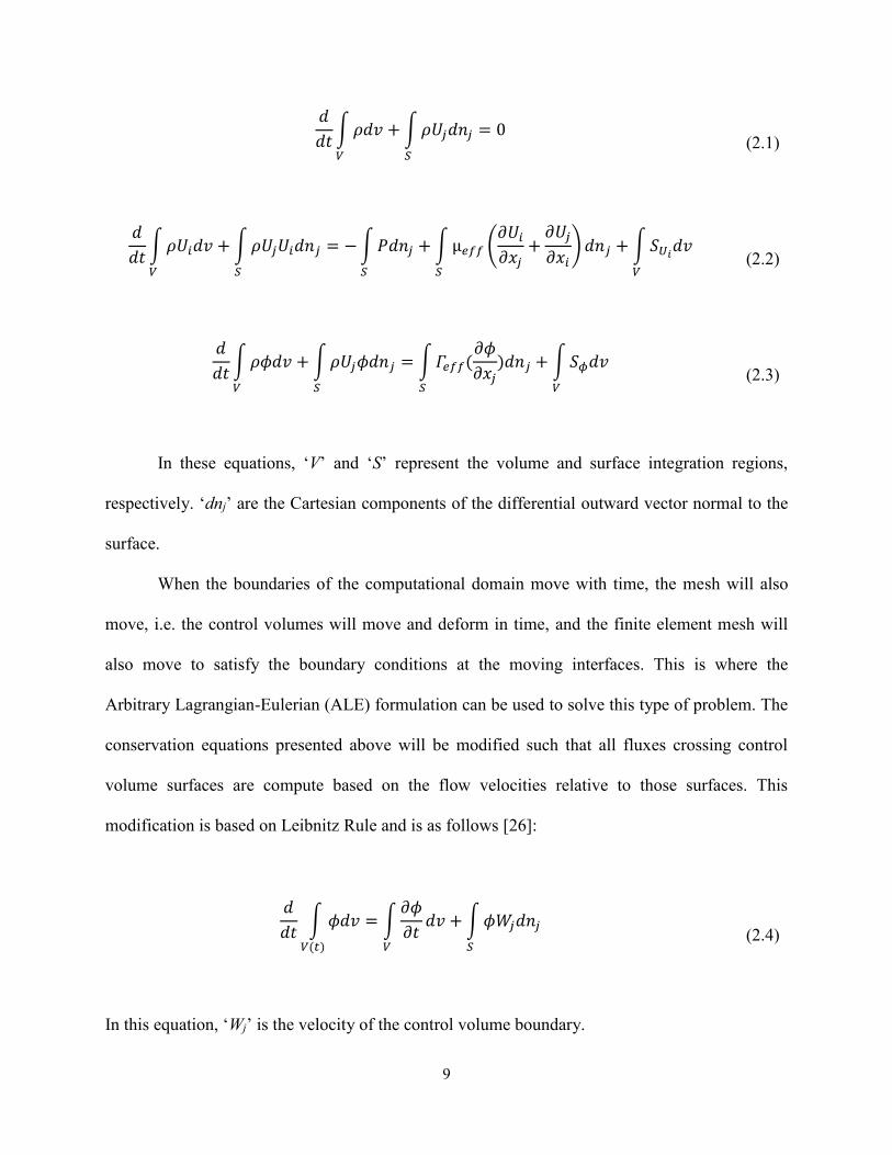
In these equations, ‘V’ and ‘S’ represent the volume and surface integration regions,

respectively. ‘dnj’ are the Cartesian components of the differential outward vector normal to the

surface.

When the boundaries of the computational domain move with time, the mesh will also

move, i.e. the control volumes will move and deform in time, and the finite element mesh will

also move to satisfy the boundary conditions at the moving interfaces. This is where the

Arbitrary Lagrangian-Eulerian (ALE) formulation can be used to solve this type of problem. The

conservation equations presented above will be modified such that all fluxes crossing control

volume surfaces are compute based on the flow velocities relative to those surfaces. This

modification is based on Leibnitz Rule and is as follows [26]:

𝑑

𝑑𝑡∫ 𝜙𝑑𝑣

𝑉(𝑡)

= ∫𝜕𝜙

𝜕𝑡𝑑𝑣

𝑉

+ ∫ 𝜙𝑊𝑗𝑑𝑛𝑗

𝑆

(2.4)

In this equation, ‘Wj’ is the velocity of the control volume boundary.

10

After applying the Leibnitz Rule to Eqs. (2.1), (2.2) and (2.3) they will be written as [26]:

𝑑

𝑑𝑡∫ 𝜌𝑑𝑣

𝑉(𝑡)

+ ∫ 𝜌(𝑈𝑗 − 𝑊𝑗)𝑑𝑛𝑗

𝑆

= 0 (2.5)

𝑑

𝑑𝑡∫ 𝜌𝑈𝑖𝑑𝑣

𝑉(𝑡)

+ ∫ 𝜌(𝑈𝑗 − 𝑊𝑗)𝑈𝑖𝑑𝑛𝑗 =

𝑆

− ∫ 𝑃𝑑𝑛𝑗

𝑆

+ ∫ µ𝑒𝑓𝑓(𝜕𝑈𝑖

𝜕𝑥𝑗+

𝜕𝑈𝑗

𝜕𝑥𝑖)𝑑𝑛𝑗

𝑆

+ ∫ 𝑆𝑈𝑖𝑑𝑣

𝑉

(2.6)

𝑑

𝑑𝑡∫ 𝜌𝜙𝑑𝑣

𝑉(𝑡)

+ ∫ 𝜌(𝑈𝑗 − 𝑊𝑗)𝜙𝑑𝑛𝑗

𝑆

= ∫ 𝛤𝑒𝑓𝑓(𝜕𝜙

𝜕𝑥𝑗)𝑑𝑛𝑗

𝑆

+ ∫ 𝑆𝜙𝑑𝑣

𝑉

(2.7)

Eqs. (2.5), (2.6) and (2.7) are referred to as the Unsteady Reynolds averaged Navier-

Stokes equations written in an Arbitrary Lagrangian-Eulerian (ALE) formulation to account for

the mesh deformation. In these equations, ‘𝜇𝑒𝑓𝑓’ is the effective viscosity which is the sum of

molecular (dynamic) and turbulent viscosity. ‘Γ𝑒𝑓𝑓’ is the effective diffusivity, and ‘𝜙’ is the

total energy per unit mass. Furthermore, ‘𝑆𝑈𝑖’ and ‘𝑆𝜙’ are the momentum and energy source

terms, respectively; they are set to zero in this study as there is no heat generation and no body

forces in the computational domain.

The turbulence model used in this work is the standard 𝑘 − 𝜔 model which is widely

used in turbomachinery applications. The advantage of using this model over other two-equation

turbulence models is the accurate prediction of flow separation which is crucial in the scope of

this work. Turbulence models based on 휀-equation typically fail to predict accurately the onset

and extent of the separated region under adverse pressure gradients. As a result, these models

11

usually over-predict the performance in such cases and are not reliable enough. Another merit of

using 𝑘 − 𝜔 turbulence model is the ability to have near wall treatment for low-Reynolds

numbers. In CFX, there is ‘Automatic Near-wall Treatment’ option for 𝜔 -based turbulence

models which allows a smooth change from low-Reynolds number form to an appropriate wall

function formulation. This is the default option in CFX for all 𝜔-based models including 𝑘 − 𝜔

and results in avoiding numerical instabilities and errors observed in other models near the wall.

It must also be mentioned that the convergence behavior of the 𝑘 − 𝜔 model is usually similar to

𝑘 − 휀 model [26].

The flow simulation were carried out for both steady and unsteady states. In analysis

mode, where the blade profile is given, the flow field is assumed to be steady and the Reynolds

averaged Navier-Stokes (RANS) equations are solved. On the other hand, in the design mode

where the blade shape changes from an initial guess to one that satisfies the target design

variables, the problem is unsteady due to the blade motion. In this case, the unsteady Reynolds

averaged Navier-Stokes (URANS) equations, written for a moving and deforming mesh, are

solved for the flow field around the blade.

A second-order scheme which is recommended by ANSYS-CFX for turbomachinery

applications was used for the URANS equations, and a first order scheme was used for

turbulence. The second order accurate backward Euler scheme is chosen to march the equations

in time. This is an implicit time stepping scheme which is recommended by ANSYS-CFX to be

used in most transient simulations [26].

12

2.1.1 User Defined Function

ANSYS-CFX solves the flow governing equations during the design process and provides the

flow properties in the whole computational domain. The inverse design methodology on the

other hand must be embedded into ANSYS-CFX in order to implement the inverse design. This

task is done using a user ‘CFX Expression Language’ CEL function. An external FORTRAN

routine containing the inverse design formulation is written and is linked to CFX. This user CEL

function is called at each physical time step, and receives the computed flow properties and grid

geometry from CFX as input. The output of the CEL is the new coordinates of the airfoil which

are computed based on the displacement obtained from inverse design. These coordinates are

then passed to CFX for re-meshing and solving the flow field over the new geometry. This

procedure is repeated until convergence is reached [13].

2.1.2 Mesh Motion

In inverse design, the blade surface is continuously updated by imposing a displacement field

which is computed based on the difference between the current and target pressure distributions

on the blade. In other words, the mesh must move and deform in the time accurate simulation.

The available options for mesh deformation in ANSYS-CFX are as follows [26]:

None

Junction Box Routine

Regions of Motion Specified

13

The first option is used when there is no mesh movement. When the Junction Box Routine

option is chosen, a User Fortran routine must be specified to explicitly set the coordinates of all

nodes in the computational domain.

The last option is ‘Regions of Motion Specified’. This options allows user to define the

motion of the grid points on boundary or subdomain regions of the mesh using CEL, while CFX

will compute the motion of the rest of the domain nodes by the mesh motion model. Currently,

the available mesh motion model in CFX is ‘Displacement Diffusion’. This model diffuses the

applied displacement on boundary or subdomain regions to the rest of the mesh nodes by solving

Eq. (2.8):

∇. (Γdisp. ∇δ) = 0 (2.8)

In this equation, ‘δ’ is the displacement relative to the previous mesh nodes and ‘Γdisp’ is the

mesh stiffness which specifies the degree to which regions of mesh nodes are displaced together.

In the scope of this work, the displacement of the nodes on the blade boundary is directly

computed in a CEL function as was mentioned in section 2.1.1, and the displacement of the rest

of the domain is unspecified. Consequently, the most appropriate option to be used in this work

is the ‘Regions of Motion Specified’.

14

2.1.3 Mesh Stiffness

Mesh stiffness specifies how the imposed displacements must be diffused throughout the

mesh. Mesh stiffness can either be a constant value or varying throughout the domain. In the first

case, the mesh diffusion will be homogenous in the entire domain. However, in the latter case the

relative motion of the mesh nodes will be smaller in regions of higher stiffness. This options is

beneficial to preserve the mesh quality and density in regions such as boundary layer. There are

two types of varying mesh stiffness in CFX [26]:

Increase Near Small Volumes: The mesh stiffness increases exponentially as control

volume size (mesh size) decreases. The mesh stiffness is computed from the following relation:

Γdisp = (∀𝑟𝑒𝑓

∀)

𝐶𝑠𝑡𝑖𝑓𝑓

(2.9)

In this relation, ‘∀’ is the control volume size and ‘∀𝑟𝑒𝑓’ is the reference volume which is

set to 1 [m3] by default. ‘𝐶𝑠𝑡𝑖𝑓𝑓’ is the stiffness model exponent which determines how fast the

stiffness increase must occur. Higher values will represent more abrupt changes in stiffness.

Increase Near Boundaries: The mesh stiffness increases near certain boundaries

such as wall, inlet, outlet and opening. The merit of using this option is that mesh

quality is preserved near boundaries. The following relation is used to obtain the

mesh stiffness:

15

Γdisp = (𝐿𝑟𝑒𝑓

𝑑)

𝐶𝑠𝑡𝑖𝑓𝑓

(2.10)

In this relation, the mesh stiffness increases as the distance from the nearest boundary, 𝑑,

decreases. ‘𝐶𝑠𝑡𝑖𝑓𝑓’ is the stiffness model exponent and ‘𝐿𝑟𝑒𝑓’ is the reference length which is set

to 1 [m] by default. This option also needs an additional boundary scale equation to be solved.

In this work, the option “Increase Near Boundaries” is used in order to preserve the mesh

quality near boundaries; specifically at the boundary layer around the blade wall.

2.1.4 Mesh Considerations

A multi-block grid topology has been used to discretize the computational domain. To ensure

resolving the boundary layer and providing numerical results with as a high accuracy as possible,

an O-grid topology has been used in the vicinity of the blade wall. This will provide an

orthogonal grid with a higher quality. Furthermore, the value of y+ has been carefully monitored

and is less than one which guarantees a suitable resolution of the boundary layer. The rest of the

numerical domain is filled with a structured mesh.

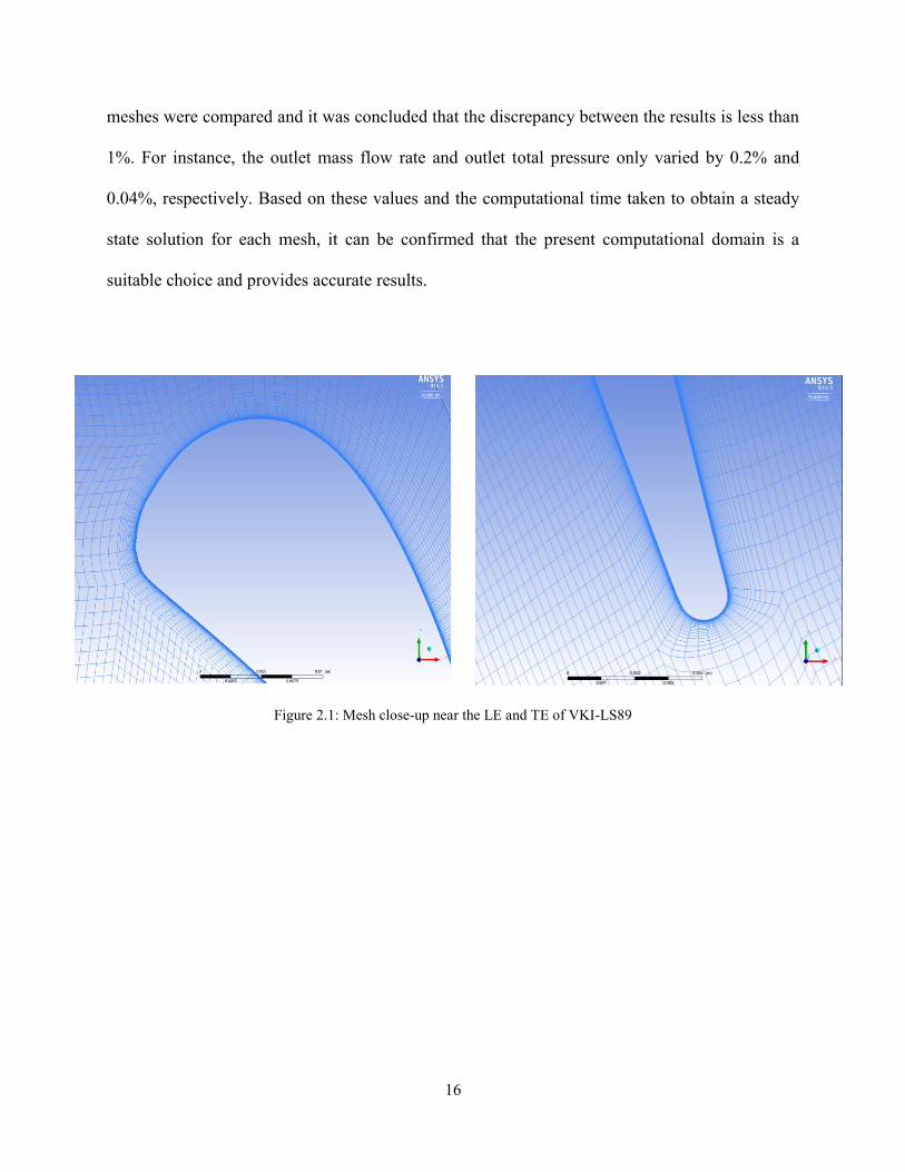
Figure 2.1 shows the computational grid close-up near the LE and TE regions of VKI-

LS89. The total number of elements for this computational grid is 78,077. In order to ensure the

independency of the results from the mesh, the number of elements was increased to 461,276

which is 5.9 times the number of elements for the current mesh. Most of the nodes were added at

the LE and TE regions as well as the rear part of the blade. The steady state results from two

16

meshes were compared and it was concluded that the discrepancy between the results is less than

1%. For instance, the outlet mass flow rate and outlet total pressure only varied by 0.2% and

0.04%, respectively. Based on these values and the computational time taken to obtain a steady

state solution for each mesh, it can be confirmed that the present computational domain is a

suitable choice and provides accurate results.

Figure 2.1: Mesh close-up near the LE and TE of VKI-LS89

17

2.2 Inverse Design Methodology

The inverse blade shape design methodology that was developed by Daneshkhah and Ghaly [11,

12] and was demonstrated for 2D flow will be briefly presented in this section. In this inverse

method, the momentum flux balance resulting from the difference between the current and target

pressure distributions on the blade is the source of computing a virtual wall velocity for the

blade. The blade surface moves with this fictitious velocity up to the point where the difference

between the current and target pressure distributions on the blade surface is very small, i.e. the

virtual wall velocity approaches zero. The new blade shape resulting from this method produces

the target pressure specified at the beginning of the design process.

This approach is fully consistent with the viscous flow assumption. The flow is unsteady

due to the blade movement and is solved using a time accurate scheme. The flow field over the

blade is computed by solving the URANS equations written in Arbitrary Lagrangian-Eulerian

(ALE) form to account for the blade movement and deformation.

There are several choices of design variables, three of these choices are listed here.

Choice 1: the tangential blade thickness and pressure distribution on the blade SS; Choice 2: the

tangential blade thickness and blade pressure loading; Choice 3: the pressure distributions on the

blade SS and PS. The choice of the design variable(s) depends on the designer’s intent.

18

2.2.1 Inverse Design Formulation

The virtual wall velocity for the blade surface is computed based on the difference between the

current and target pressure distributions. Assuming 2D flow, and a virtual velocity vector 𝒗𝒗 =

(𝑢𝑣, 𝑣𝑣), the transient momentum flux, F, on the blade surfaces is given by [27]:

𝐹 = [(𝜌𝑢𝑣𝑢𝑣 + 𝑃)𝑛𝑥 + (𝜌𝑢𝑣𝑣𝑣)𝑛𝑦

(𝜌𝑢𝑣𝑣𝑣)𝑛𝑥 + (𝜌𝑣𝑣𝑣𝑣 + 𝑃)𝑛𝑦]

(2.11)

In Eq. (2.11), 𝒏 = (𝑛𝑥, 𝑛𝑦) is the surface normal vector. As the target pressure is reached

on the blade, the virtual wall velocity vanishes and the only contribution to the momentum fluxes

on the designed blade is due to the design pressure, 𝑃𝑑. Hence, the design momentum flux will

take the following form:

𝐹𝑑 = [

(𝑃𝑑𝑛𝑥)

(𝑃𝑑𝑛𝑦)]

(2.12)

The virtual velocity can be obtained by equating Eq. (2.11) and (2.12), that is:

𝐹 = 𝐹𝑑 (2.13)

Then, the velocity components can be directly computed from Eq. (2.13).

𝑣𝑣 = ± (𝑛𝑦

2

𝑛𝑥2 + 𝑛𝑦

2

|𝑃𝑑 − 𝑃|

𝜌)

12

(2.14)

𝑢𝑣 = 𝑣𝑣

𝑛𝑥

𝑛𝑦

(2.15)

19

In case when there is a positive difference between the target and current pressure on

each side of the blade, a positive wall velocity is imposed for balance. For convenience, only the

virtual velocity component normal to the wall is taken as the wall velocity. That is:

𝑣𝑣,𝑛 = 𝒗𝒗. n (2.16)

The wall displacement ‘𝛿𝑠’ in a physical time interval ‘𝛿𝑡’ can be computed as:

𝛿𝑠 = −𝜔𝛿𝑡𝑣𝑣,𝑛 (2.17)

The negative sign in Eq. (2.17) represents a movement in the opposite direction of 𝑣𝑣,𝑛,

and ‘𝜔’ is a relaxation factor that is used to ensure the scheme stability and convergence to a

steady state solution [28]. This relaxation factor takes the following form:

𝜔 = 휀. (1𝑐⁄ )√|𝛥𝑃|/𝜌

(2.18)

In this equation, ‘c’ is the speed of sound, ‘𝛥𝑃’ is the difference between the target and

actual pressure distributions, and ‘휀’ is a constant that varies between 0.01 and 0.02 for transonic

flow [29], and for subsonic flow it varies between 0.1 and 0.2 [27, 30].

The node displacements computed from Eq. (2.17) are applied to discrete grid points on

the blade surface, that is:

𝑥𝑛± = 𝑥𝑜

± + 𝛿𝑥± (2.19)

𝑦𝑛± = 𝑦𝑜

± + 𝛿𝑦± (2.20)

20

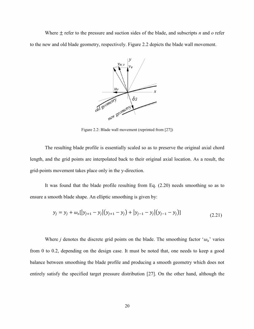
Where ± refer to the pressure and suction sides of the blade, and subscripts n and o refer

to the new and old blade geometry, respectively. Figure 2.2 depicts the blade wall movement.

Figure 2.2: Blade wall movement (reprinted from [27])

The resulting blade profile is essentially scaled so as to preserve the original axial chord

length, and the grid points are interpolated back to their original axial location. As a result, the

grid-points movement takes place only in the y-direction.

It was found that the blade profile resulting from Eq. (2.20) needs smoothing so as to

ensure a smooth blade shape. An elliptic smoothing is given by:

𝑦𝑗 = 𝑦𝑗 + 𝜔𝑠[|𝑦𝑗+1 − 𝑦𝑗|(𝑦𝑗+1 − 𝑦𝑗) + |𝑦𝑗−1 − 𝑦𝑗|(𝑦𝑗−1 − 𝑦𝑗)] (2.21)

Where j denotes the discrete grid points on the blade. The smoothing factor ‘𝜔𝑠’ varies

from 0 to 0.2, depending on the design case. It must be noted that, one needs to keep a good

balance between smoothing the blade profile and producing a smooth geometry which does not

entirely satisfy the specified target pressure distribution [27]. On the other hand, although the

21

smoothing factor can increase the convergence time, but it can remove small oscillations in the

geometry [30].

There is also another design option which enables the user to specify the target pressure

loading distribution and the blade tangential thickness distribution. In this case, the average

displacement of both blade surfaces is added to the camber line, that is:

𝑓(𝑥)𝑛 = 𝑓(𝑥)𝑜 ± 0.5(𝛿+ + 𝛿−) (2.22)

Where ‘f’ denotes the blade camber line.

In order to achieve a smooth camber line which leads to having a smooth blade profile,

one or two elliptic smoothing cycles (similar to Eq. (2.21)) should be applied on the camber line.

The new blade profile is then constructed by adding the specified thickness to the designed

camber line as follows:

𝑦(𝑥)𝑛± = 𝑓(𝑥)𝑛 ± 0.5𝑇(𝑥)𝑜

(2.23)

2.2.2 Design Variables

There are three different options for the choice of design variables within the user defined

function. They will be briefly explained.

The first option is to specify the target pressure distributions on the blade suction and

pressure surfaces. In this case, the wall virtual velocity and displacement are computed from Eqs.

22

(2.15), (2.16) and (2.17). The blade thickness is not specified in this option and will be obtained

as part of the design solution. This may cause structural problems in the designed blade which

can be prevented by preserving the original blade shape in small regions at the blades leading

and trailing edges [30].

The second design option is to prescribe the pressure loading and tangential thickness

distribution. However, one needs to find the target pressure distribution on the suction and

pressure surfaces to be able to use Eq. (2.14) to compute the wall virtual velocities. The

following relation is used to find the corresponding target static pressure distribution based on

the prescribed pressure loading:

𝑃 ± =

1

2[(𝑃+ + 𝑃−) ± 𝛥𝑃 ] (2.24)

In this equation, 𝑃+ and 𝑃− are the static pressure distributions on the blade pressure side

and suction side computed from the flow governing equations at the beginning of each design

time step.

The other design variable in this option, is the blade tangential thickness distribution. In

order to achieve the target thickness, the blade camber line is displaced in each design step using

Eq. (2.22), and the specified thickness distribution is imposed on the updated camber line using

Eq. (2.23). This was explained in detail in section 2.2.1.

The last option is to prescribe the target pressure distribution on the suction side and the

tangential thickness distribution. This option has been provided to enable the designer to have

more control over the blade performance. The flow on the blade pressure side is often well

behaved and thus having it modified will not have a decisive effect on the blade performance.

23

However, one can improve the blade performance by tailoring the pressure distribution on the

suction side as it has a dominant effect on the blade losses. The other design variable is the

tangential blade thickness; it will be imposed similar to the previous option.

2.2.3 Design Considerations

There are geometric and non-geometric constraints which must be respected during the inverse

design process. Some of the non-geometric constraints such as inlet flow angle, mass flow rate,

inlet total temperature, and outlet static pressure can be respected by the correct choice of the

inflow and outflow boundary conditions.

Some geometric constraints such as the number of blades, and the chord length are

readily satisfied in the current inverse design method [27]. Two other geometric constraints

including the LE/TE shapes can be obtained by preserving the blade shape in these regions. For

this purpose, the blade shape near the LE and TE, will not go through inverse design and is ran in

analysis mode. The length of the preserved portions near the LE and TE can vary between 1%

and 5% of the chord length for different geometries. This approach will avoid possible

crossovers in the TE region, or an open shape at the LE which might be a result of the arbitrary

choice of the target pressure distribution [30]. In order to ensure a smooth profile at the transition

point between the preserved portion and the designed portion of the blade, the slope of the

camber line and the blade tangential thickness in the preserved portion are matched with the ones

prevailing in the designed portion [23].

24

Chapter 3

3 Airfoil Shape and Design Variables Representation and

Modification

In each inverse design step, the airfoil shape must be interpolated using discrete grid points and

updated after imposing the computed displacements.

In addition to the airfoil geometry, interpolation must be carried out for the flow variables

on the blade. To elaborate, in case of specifying a target pressure loading distribution, the values

of the target pressure are not necessarily given in the position of the grid points on the blade

wall. In order to proceed with the calculation of the wall virtual velocity, the value of the target

pressure at the grid points on both sides of the blade must be known (for more details see

section 2.2.2). This can only be done by using an interpolation tool to find the values of the

target pressure at the grid points.

On the other hand, the first step in inverse design is to specify either a target static

pressure or a target pressure loading distribution for the blade. In other words, the designer needs

to start the inverse design with tailoring the target pressure distribution on the blade so as to

achieve certain design goals. Some of these goals could be minimizing losses, reducing the

adverse pressure gradient, and modifying the onset and/or extent of the flow separation. To do

so, one needs a robust interpolation tool to modify the analysis pressure (or pressure loading)

distribution on the blade.

25

Considering the above-mentioned requirements, one robust interpolation method is

needed throughout this work. There are different ways of interpolating discrete data. The most

rudimentary way is to fit a polynomial curve which passes through all the data points. However,

there are various shortcomings for such curves which are only consisted of one polynomial

segment. To name a few, a high degree is required to precisely fit a curve to data points

corresponding to complex shapes and to satisfy the geometry constraints. Also, the resulting

curve might not be as accurate as required. A good way to get around these problems is to use

curves which consist of different polynomial segments instead of one segment. A robust

powerful tool which has this feature is the B-Spline function. A B-spline curve is a congregate of

continuous piecewise polynomials each covering a portion of the total interval; these portions are

overlapping.

B-splines can be used to represent arbitrary complex shapes, they are becoming the

industry standard in representing curves and shapes in CAD files. They are very efficient to

process and suitable for interactive shape design, simple to implement and can generate curves

with high levels of precision. As B-spline continuity is determined by its Basis functions (For

more details, see Appendix A), one can modify the curve locally without affecting its global

shape and continuity. Furthermore, the curve smoothness will be maintained. B-Splines are also

one of the most robust, reliable and flexible interpolation methods available in the CAD industry

nowadays. Considering all these benefits, B-splines have been used in the scope of this work to

represent both geometry and design variables.

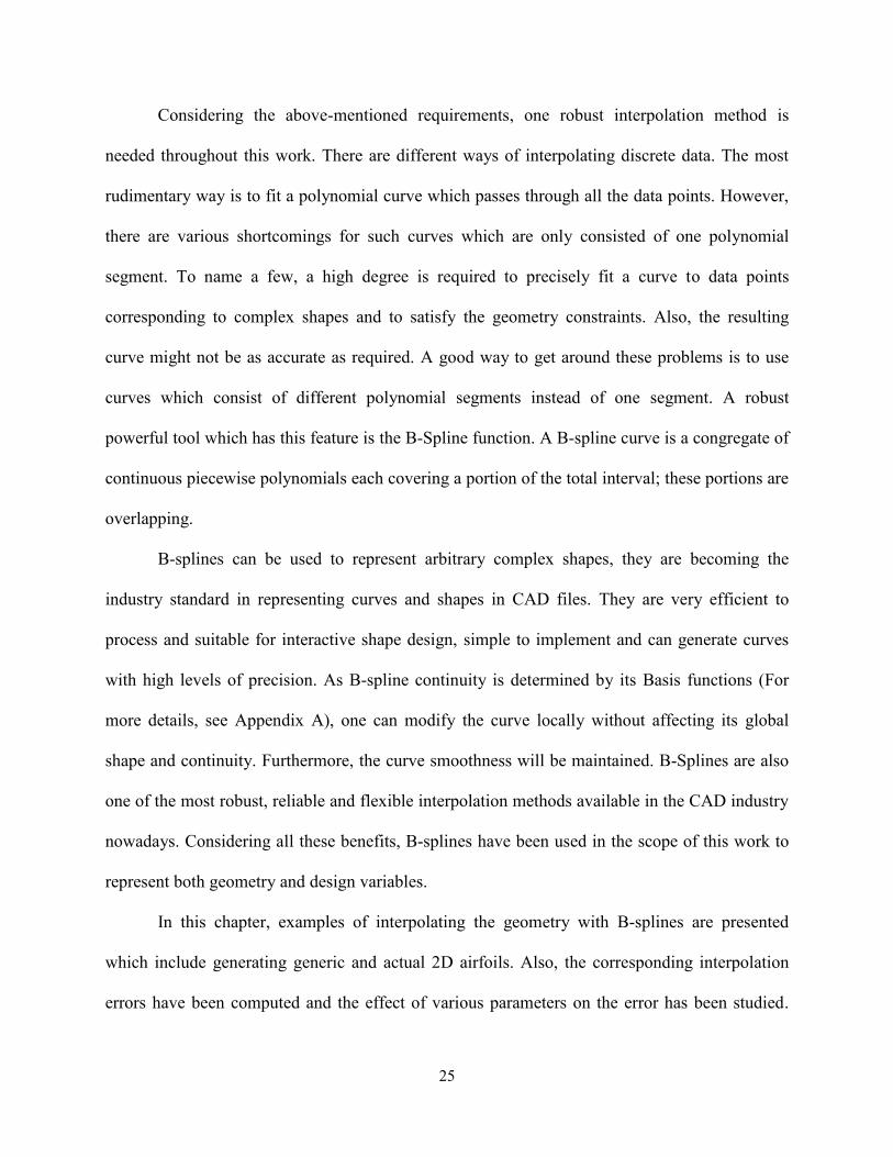
In this chapter, examples of interpolating the geometry with B-splines are presented

which include generating generic and actual 2D airfoils. Also, the corresponding interpolation

errors have been computed and the effect of various parameters on the error has been studied.

26

Later in this chapter, representation of design variables by B-splines is clarified. B-spline curve

preliminaries are presented in Appendix A.

3.1 Representation of 2D Airfoils with B-Splines

As it was mentioned earlier, B-Splines are used in this work to generate the airfoil geometry. To

evaluate the robustness and accuracy of B-splines, three cases are studied. One is a generic

compressor blade and the other two are given by actual compressor blades; E/CO-1 and Rotor

67. Furthermore, the effect of clustering the control points, number of control points, and curve

degree on the accuracy of the results are studied.

The procedure is to fit a B-spline to a series of initial data points (x- and y-coordinates of

the airfoil). Once the B-spline is fitted and the control points are obtained, the error can be

calculated using more number of initial data points on the curve.

There are various ways of defining the error. In this case, the error at each point on the

actual curve is calculated based on the minimum (perpendicular) distance between that point and

the B-spline curve. The average error is defined in Eq. (3.1).

𝑒𝑎𝑣𝑒𝑟𝑎𝑔𝑒 =1

𝑚∑ 𝑒𝑖

𝑚

𝑖=1

(3.1)

Also, the L2-norm is defined as follows.

𝐿2 − 𝑛𝑜𝑟𝑚 = √∑ 𝑒𝑖2

𝑚

𝑖=1

(3.2)

27

The required level of precision to represent the blade shape is set based on the

manufacturing tolerance and/or the change in aerodynamic performance. In the case of a gas

turbine blade with one inch chord, this value should be around 2×10-4 [31].

3.1.1 Generic Blade

The following analytical profile is used to create the airfoil shape [31].

𝑦±(𝑥) = 𝑓(𝑥) ±𝑇(𝑥)

2 (3.3)

Where

𝑓(𝑥) =1

2(tan 𝛽2 − tan 𝛽1)𝑥2 + 𝑥 tan 𝛽1

𝑇(𝑥) = 2𝑇𝑚𝑎𝑥√𝑥(1 − 𝑥)

(3.4)

𝑦± represent the blade shape on the pressure and suction surfaces, 𝑓(𝑥) is the camber

line, and 𝑇(𝑥) is the thickness distribution characterized by round LE and TE; 𝛽1 and 𝛽2 are the

blade angles at the LE and TE, respectively.

The generic compressor airfoil which is generated using the above-mentioned analytical

profile has a round LE and a sharp TE. It has a maximum thickness of 𝑇𝑚𝑎𝑥 =15%, a unit chord

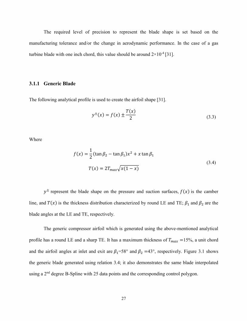
and the airfoil angles at inlet and exit are 𝛽1=58° and 𝛽2 =43°, respectively. Figure 3.1 shows

the generic blade generated using relation 3.4; it also demonstrates the same blade interpolated

using a 2nd degree B-Spline with 25 data points and the corresponding control polygon.

28

Figure 3.1: Generic compressor profile; 25 Control points, 2nd degree

Table 3.1 summarizes the error of interpolation for different number of input points. 300

data points are used to calculate the error in all the cases. It must be noted that input points for

interpolation are carefully selected based on the curvature distribution; i.e. more input points

(equivalent to more CP’s) are selected in the higher curvature areas which is typically in the

leading and trailing edge regions.

Table 3.1: Error comparison for different number of control points

Number of

CP’s1

Curve degree

p

Average Error

eavg (m)

Maximum Error

emax (m)

L2-norm

(m)

25 2 1.595×10-4 7.59×10-4 4.028×10-3

30 2 8.892×10-5 5.82×10-4 2.446×10-3

40 2 3.865×10-5 4.46×10-4 1.338×10-3

50 2 3.365×10-5 3.98×10-4 1.160×10-3

1 The number of control points is the same as the number of input data points.

X

Y

0 0.2 0.4 0.6 0.8 1

0

0.2

0.4

0.6

0.8

1

1.2Generic blade

B-spline (2nd degree)

Control polygon

29

As it is expected, according to Table 3.1 the average and maximum error decrease once

the number of the control points is increased. Furthermore, the average error in all the cases is

below the manufacturing tolerance which was mentioned earlier.

3.1.2 E/CO-1 Compressor Blade

E/CO-1 is a single stage low speed compressor rotor. The x- and y-coordinates of the blade at

different span-wise locations are provided in Fottner [32]. The data used in this section

corresponds to the blade tip, i.e. 100% span and the axial chord length is 15.3×10-2 (m). Based on

the chord length, the manufacturing tolerance for this airfoil is 3×10-7 (m).

Table 3.2 shows the errors associated with the use of 40 and 45 control points for

interpolating E/CO-1. As it can be seen in this table, the interpolation error in both cases is less

than the manufacturing tolerance which proves the accuracy of the B-spline representation. It is

also observed that the error decreases with increasing the number of CP’s.

Comparing the results in Table 3.1 and Table 3.2 leads to the conclusion that a larger

number of control points is required to accurately represent an actual compressor cascade

compared to a generic one.

Table 3.2: Error comparison for different number of control points for E/CO-1 rotor

Number of

CP’s

Curve degree

p

Average Error

eavg (m)

Maximum Error

emax (m)

L2-norm

(m)

40 2 1.74×10-7 2.18×10-6 4.39×10-6

45 2 8.88×10-8 9.06×10-7 1.96×10-6

30

3.1.3 Rotor 67

The next test case is the mid-span of the NASA transonic fan which is also known as Rotor 67.

The geometry of Rotor 67 is given in Fottner [32]. The axial chord length of Rotor 67 is 9×10-2

(m). The manufacturing tolerance based on this chord length is 1.8×10-5 (m).

The errors for a quadratic B-spline fitted to 70 input points is presented in Table 3.3. As it

can be seen from the results, the average error is well below the manufacturing tolerance which

confirms the precision and reliability of B-splines in curve fitting.

Table 3.3: Error of interpolation for Rotor 67

Number

of CP’s

Curve degree

p

Average Error

eavg (m)

Maximum Error

emax (m)

L2-norm

(m)

70 2 5.73×10-6 2.43×10-5 1.09×10-5

3.1.4 Effect of Number of Control Points on the Error

The effect of the number of control points on the accuracy of the representation, can be realized

from Table 3.1 and Table 3.2. The results reveal that increasing the number of control points

would decrease the error of interpolation. However, the drawback is the need for more

computational time and memory.

It was also concluded that more control points should be used to generate an actual blade

in comparison with a generic blade. This demonstrates the importance of smooth initial data

points with least possible noise in the blade discrete shape to generate precise interpolated

profiles.

31

3.1.5 Effect of Control Points Clustering on the Error

To demonstrate the effect of clustering the control points in specific regions of the airfoil on the

interpolation error, the compressor generic blade is interpolated using two different sets of initial

data points. Both sets have the same number of control points (45 points). However, in one,

control points are clustered based on the curvature and in the other, they are distributed evenly. It

must be noted that the same curve degree has been used in both cases.

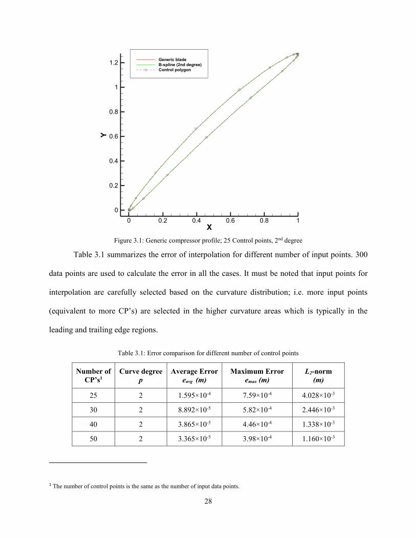
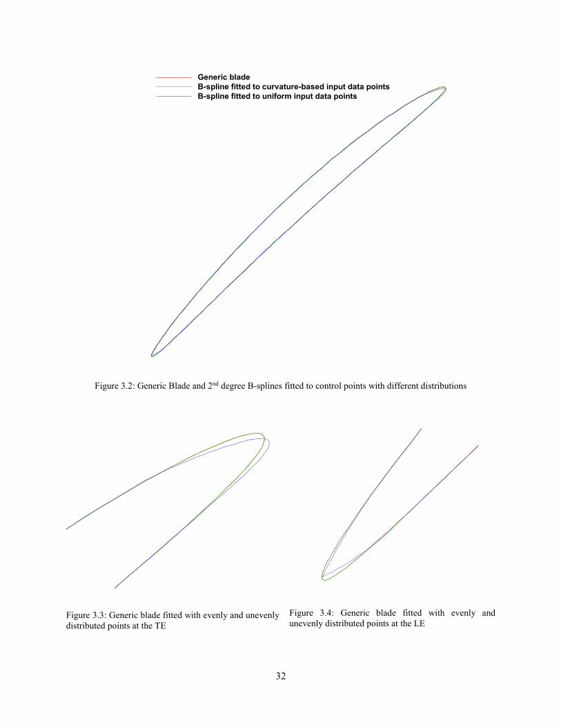
Figure 3.2 shows the generic blade, the B-spline fitted to curvature-based data and B-

spline fitted to uniformly distributed data points. Figure 3.3 and Figure 3.4 depict the same

curves closely at the trailing edge and leading edge, respectively.

As it can be seen in these figures, control points should be clustered in regions of high

curvature, such as LE and TE which implies more data points in these two regions. This is to

obtain an accurate airfoil representation. Otherwise, the fitted B-spline cannot represent the blade

shape in high curvature regions correctly and one might lose some important geometry

characteristics. As a result, curvature was considered an important criterion for the selection of

the initial data points throughout this work.

32

Figure 3.2: Generic Blade and 2nd degree B-splines fitted to control points with different distributions

Figure 3.3: Generic blade fitted with evenly and unevenly

distributed points at the TE

Figure 3.4: Generic blade fitted with evenly and

unevenly distributed points at the LE

X

Y

0 0.2 0.4 0.6 0.8 1

0

0.2

0.4

0.6

0.8

1

1.2

Generic blade

B-spline fitted to curvature-based input data points

B-spline fitted to uniform input data points

X

Y

0.85 0.9 0.95 1 1.05

1.1

1.15

1.2

1.25

1.3

1.35 Generic blade

B-spline fitted to curvature-based input data points

B-spline fitted to uniform input data points

X

Y

0 0.05 0.1 0.15-0.05

0

0.05

0.1

0.15

0.2

Generic blade

B-spline fitted to curvature-based input data points

B-spline fitted to uniform input data points

33

3.1.6 Effect of Curve Degree on the Error

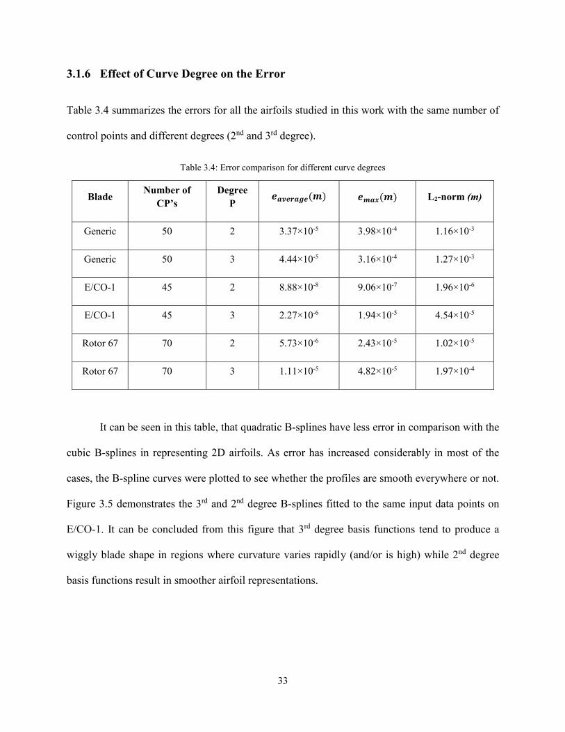
Table 3.4 summarizes the errors for all the airfoils studied in this work with the same number of

control points and different degrees (2nd and 3rd degree).

Table 3.4: Error comparison for different curve degrees

Blade Number of

CP’s

Degree

P 𝒆𝒂𝒗𝒆𝒓𝒂𝒈𝒆(𝒎) 𝒆𝒎𝒂𝒙(𝒎) L2-norm (m)

Generic 50 2 3.37×10-5 3.98×10-4 1.16×10-3

Generic 50 3 4.44×10-5 3.16×10-4 1.27×10-3

E/CO-1 45 2 8.88×10-8 9.06×10-7 1.96×10-6

E/CO-1 45 3 2.27×10-6 1.94×10-5 4.54×10-5

Rotor 67 70 2 5.73×10-6 2.43×10-5 1.02×10-5

Rotor 67 70 3 1.11×10-5 4.82×10-5 1.97×10-4

It can be seen in this table, that quadratic B-splines have less error in comparison with the

cubic B-splines in representing 2D airfoils. As error has increased considerably in most of the

cases, the B-spline curves were plotted to see whether the profiles are smooth everywhere or not.

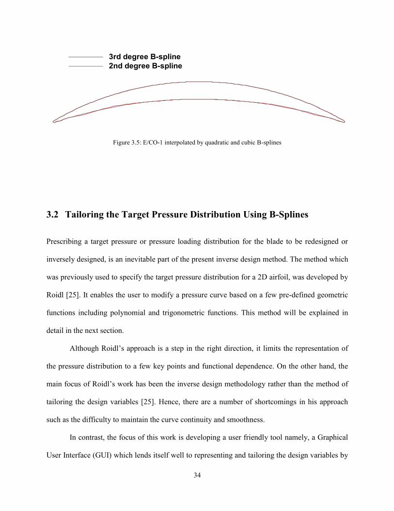
Figure 3.5 demonstrates the 3rd and 2nd degree B-splines fitted to the same input data points on

E/CO-1. It can be concluded from this figure that 3rd degree basis functions tend to produce a

wiggly blade shape in regions where curvature varies rapidly (and/or is high) while 2nd degree

basis functions result in smoother airfoil representations.

34

Figure 3.5: E/CO-1 interpolated by quadratic and cubic B-splines

3.2 Tailoring the Target Pressure Distribution Using B-Splines

Prescribing a target pressure or pressure loading distribution for the blade to be redesigned or

inversely designed, is an inevitable part of the present inverse design method. The method which

was previously used to specify the target pressure distribution for a 2D airfoil, was developed by

Roidl [25]. It enables the user to modify a pressure curve based on a few pre-defined geometric

functions including polynomial and trigonometric functions. This method will be explained in

detail in the next section.

Although Roidl’s approach is a step in the right direction, it limits the representation of

the pressure distribution to a few key points and functional dependence. On the other hand, the

main focus of Roidl’s work has been the inverse design methodology rather than the method of

tailoring the design variables [25]. Hence, there are a number of shortcomings in his approach

such as the difficulty to maintain the curve continuity and smoothness.

In contrast, the focus of this work is developing a user friendly tool namely, a Graphical

User Interface (GUI) which lends itself well to representing and tailoring the design variables by

X

Y

0 1 2 3 4 5 6

-2

-1

0

1

2

3

3rd degree B-spline

2nd degree B-spline

35

taking advantage of the B-spline key features such as continuity, smoothness and robustness. The

Graphical User Interface (GUI) developed in this work, provides the designer with more local

control over the curve shape in less time; hence saving the designer’s time and effort

considerably. This GUI enables the designer to modify the pressure (or the loading) curve

interactively by simply dragging and repositioning pre-defined control points on the screen. This

feature eliminates the need for selecting a certain geometric function by the designer to modify

the pressure distribution, unlike the previous method. This tool also has the ability to capture all

the flow physics which are implicitly implied in the pressure distribution on the blade such as

shock waves and sudden variations.

Roidl’s method [25], the B-spline approach and the GUI which is developed in the scope

of this work, will be discussed in detail in the next two sections.

3.2.1 Roidl’s Method

The method which was developed by Roidl to modify a pressure (or loading) curve is best for

making minor changes to the pressure distribution. Figure 3.6 shows a schematic of the airfoil

with the nomenclature used in this section.

The first required input for the method is the original pressure distribution on the airfoil

in the form of axial position and pressure values. Then, the regions near LE and TE where the

user chooses to preserve the original pressure distribution (given in % chord) is needed. This is

for respecting some design constraints which were mentioned in section 2.2.3. To elaborate, in

order to have a closed shape at the LE and preventing a cross-over at the TE, one needs to define

a physical pressure (or loading) distribution near these two regions. It goes without saying that

the existence of stagnation points at the LE and TE, makes it very difficult for the designer to

36

predict and specify a target pressure (or loading) distribution in these regions. To avoid such

problems, the pressure distribution is preserved in these portions and the target pressure will be

specified for the rest of the airfoil.

The user will then need to specify the location and the value of the maximum (or

minimum) pressure (or loading) coefficient, CP, and the geometric function to generate the new

target pressure with. There are four basic functions available to the user to choose from; two

weighted quadratic functions, one polynomial with x3 gradient, and a trigonometric function with

cosine gradient.

One of the key features of this routine is the ability to preserve the total loading which is

computed from the area under the pressure curve. This will prevent any structural problems

associated with the pressure forces exerted on the blade. Besides, the method has the ability to

interpolate between the original and modified pressure distributions using a user input weight in

order to capture some of the genuine properties of the original pressure curve.

After all the inputs have been fed into the routine, it would create a target pressure curve

as follows: The original pressure distribution will be preserved in the specified percentages near

the LE and TE which are called “preserved portion”. The points which exist at the boundary of

these portions are called “transition point” and the point of maximum (or minimum) CP is called

“junction point”, for simplicity. The target pressure distribution is then generated from the

transition point at the LE to the junction point, using the user’s input function and based on their

corresponding pressure values. However, the second part of the target pressure distribution from

the junction point to the transition point at the TE is created without user’s input and so as to

preserve the area under the pressure curve. For this purpose, another trigonometric function is

used to fit a smooth curve based on the values of pressure at the junction and transition point at

37

the TE. After interpolating the second part of the curve, the area under the curve is computed and

compared with the original value. The curve will then be iteratively corrected until the difference

between the areas is within a pre-defined tolerance.

Figure 3.6: Transition and Junction Points shown on the airfoil

One of the important issues in this method is smoothing the curve near the junction point,

where two functions with different tangents have been used. In order to maintain the curve’s

smoothness at this point, the value of the pressure is averaged for one point before and after the

junction point which results in a smoother transition between the two curves.

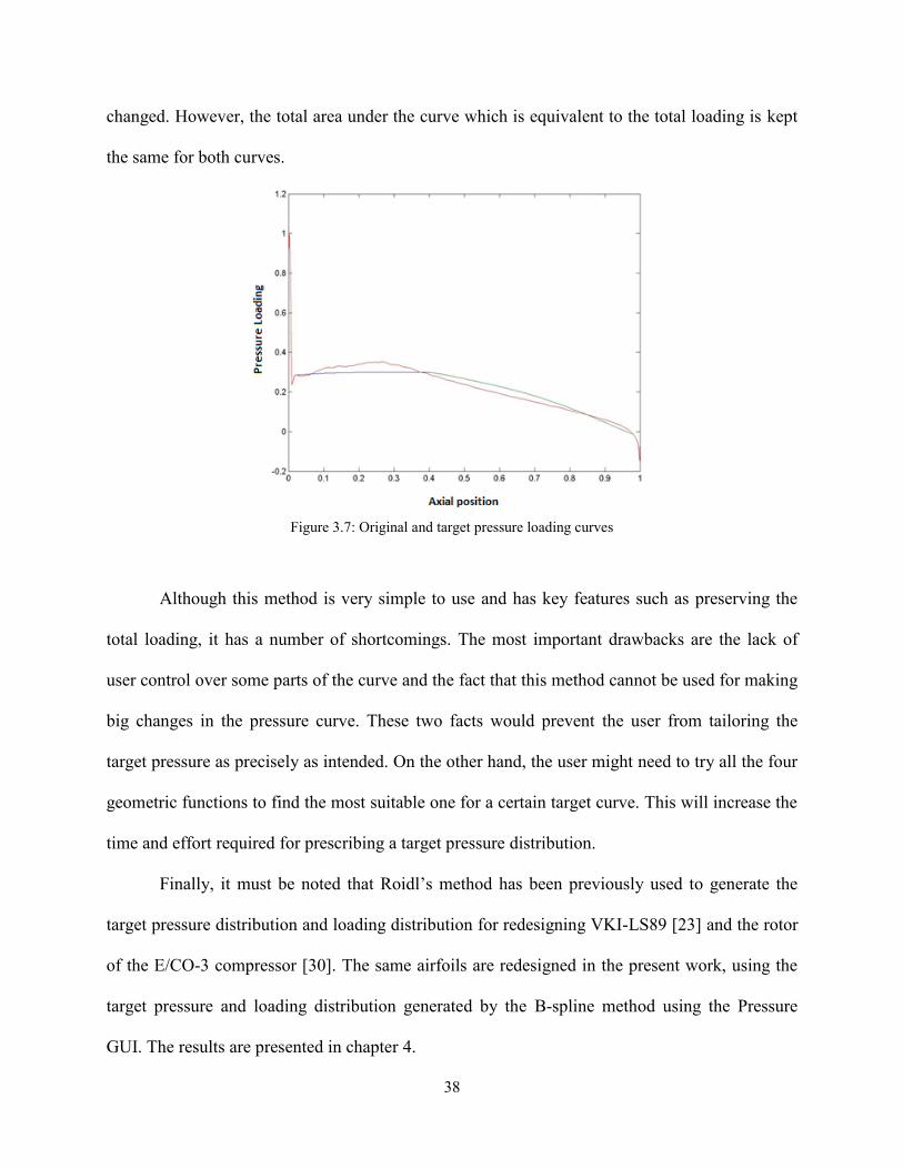
Figure 3.7 shows an analysis pressure loading (the loading arising from analyzing the

flow around a given blade) and the corresponding design (or target) loading curve which has

been prescribed by the user. The red curve gives the original loading while the other one shows

the target pressure loading. Different colors are used for the target loading in order to distinguish

the parts before and after the junction point which have been interpolated using different

geometric functions. As it can be seen in this figure, the pressure loading has not been modified

in the first and last 2% of the airfoil. Also, the location and value of the maximum CP has been

38

changed. However, the total area under the curve which is equivalent to the total loading is kept

the same for both curves.

Figure 3.7: Original and target pressure loading curves

Although this method is very simple to use and has key features such as preserving the

total loading, it has a number of shortcomings. The most important drawbacks are the lack of

user control over some parts of the curve and the fact that this method cannot be used for making

big changes in the pressure curve. These two facts would prevent the user from tailoring the

target pressure as precisely as intended. On the other hand, the user might need to try all the four

geometric functions to find the most suitable one for a certain target curve. This will increase the

time and effort required for prescribing a target pressure distribution.

Finally, it must be noted that Roidl’s method has been previously used to generate the

target pressure distribution and loading distribution for redesigning VKI-LS89 [23] and the rotor

of the E/CO-3 compressor [30]. The same airfoils are redesigned in the present work, using the

target pressure and loading distribution generated by the B-spline method using the Pressure

GUI. The results are presented in chapter 4.

39

3.2.2 Graphical User Interface

The Pressure GUI was developed to generate and modify interactively target pressure curves

and/or surfaces. It is imperative to have this tool as it allows for the generation and control of a

smooth profile for the design variables. A GUI (which is sometimes referred to as UI) is a

Graphical User Interface which enables one to have point-and-click control over software

applications. As a result, the user will not need to type commands or learn any languages to run

such an application.

The Pressure GUI was generated in MATLAB for a number of reasons; most important is

the possibility to create MATLAB GUIs interactively. To elaborate, one can graphically design a

GUI using the GUIDE layout editor. In this option, GUIDE would automatically create the

required code for building the UI and the code developer would only need to include the code for

the desired application in the UI body. Besides, MATLAB as a coding language is easy to

access, it is user friendly, and simple to learn and implement. These advantages will also enable

the user to easily modify the GUI based on additional specific requirements in the future.

The Pressure GUI is used for two main purposes: generating a target pressure curve (or

pressure surface2 in 3D flow) and interpolating the pressure on that surface. In other words, the

Pressure GUI not only enables one to modify and create a curve interactively, but it also enables

the user to specify a target pressure (or loading) for more than one span-wise section along a 3D

blade and generate a target pressure surface for the whole blade. Note that Roidl’s routine was

developed for inverse design in 2D flow only.

2 This option and its application is explained in details in Appendix B.

40

As it was explained in section 3.2, B-splines have significant features which make them a

suitable choice for curve and surface fitting, and modification applications. One of the most

fundamental features of B-splines, is the modification of a curve and/or surface locally without

compromising the shape continuity and smoothness. This is solely performed through moving

the CP’s of a curve or surface in all possible directions. Consequently, in the current GUI the

curves are fitted using B-Splines and Global Surface Interpolation method is applied to generate

surfaces3.

Figure 3.8 depicts a part of the developed Pressure GUI which demonstrates a sample

loading curve and the corresponding user-defined target. In this figure, the blue curve is an

original loading and the red one is the hypothetical target loading which has been obtained by

manipulating the pre-defined blue dotted CP’s shown on the screen.

More explicitly, in order to modify a curve, a fixed number of CP’s that can be moved

using the mouse are generated along the x-axis (axial direction) and are used to create a default

curve. The user is then able to manipulate these points to generate a target curve, i.e. drag and

drop CP’s in the desired positions to change the curve shape. The code is capable of preserving

the original area under the pressure or loading curve.

Unlike Roidl’s routine, there is no option to preserve the curve shape in user-defined

regions in this UI. The reason is the fact that these portions of the blade would eventually be

replaced by their original shape inside the CEL function in each inverse design step. Thus, the

target pressure or loading distribution specified in these portions will be automatically ignored.

3 For more details about this method, see Appendix A.

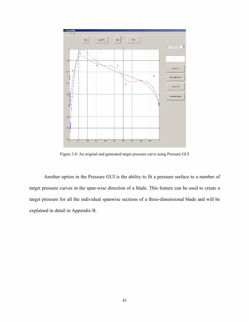
41

Figure 3.8: An original and generated target pressure curve using Pressure GUI

Another option in the Pressure GUI is the ability to fit a pressure surface to a number of

target pressure curves in the span-wise direction of a blade. This feature can be used to create a

target pressure for all the individual spanwise sections of a three-dimensional blade and will be

explained in detail in Appendix B.

42

Chapter 4

4 Inverse Design Algorithm and Redesign Results

As mentioned in section 2.1.1, the inverse design methodology is embedded into CFX by means

of a user CEL “CFX Expression Language” function. This user defined function is a subroutine

written in FORTRAN containing the inverse design formulation, it is attached to CFX and it is

compiled at the beginning of each inverse design process.

The first step before beginning the inverse design calculation, is to obtain the steady state

flow solution for the original geometry. The converged solution will be used as the initial guess

in the transient design simulation where the source of unsteadiness is the blade movement.

Furthermore, the original pressure and/or loading distribution on the blade obtained from the

steady state solution, will be assessed and the target design variable(s) can be chosen based on

the designer’s evaluation. For instance, if the flow is well behaved on the pressure side one might

choose the pressure on the suction side and the tangential thickness as the design variables. Then,

the developed Pressure GUI must be used for tailoring the chosen design variable so as to

achieve certain design goals. After specifying the target pressure or loading distribution, one can

perform the inverse design.

The inverse design process is carried out as follows. At the initial time step, the

converged steady state solution obtained for the original geometry is used as the initial value.

Then, ANSYS-CFX solves the URANS equations for the stationary blade geometry for a certain

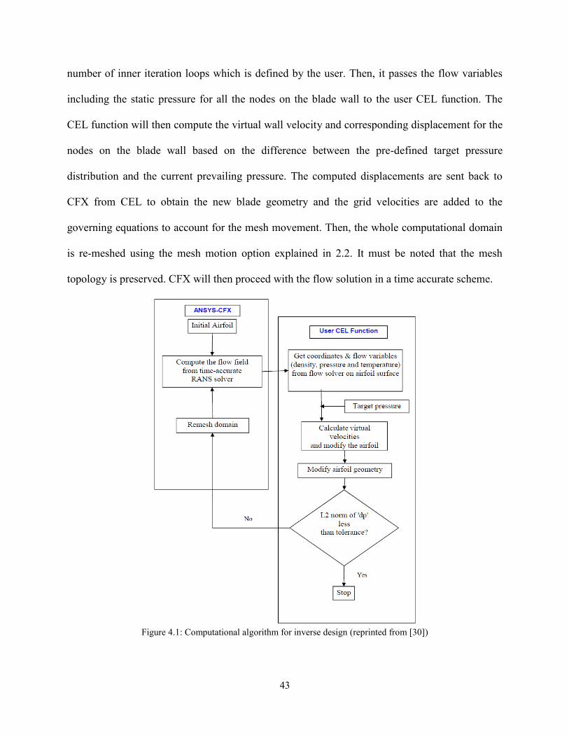
43

number of inner iteration loops which is defined by the user. Then, it passes the flow variables

including the static pressure for all the nodes on the blade wall to the user CEL function. The

CEL function will then compute the virtual wall velocity and corresponding displacement for the

nodes on the blade wall based on the difference between the pre-defined target pressure

distribution and the current prevailing pressure. The computed displacements are sent back to

CFX from CEL to obtain the new blade geometry and the grid velocities are added to the

governing equations to account for the mesh movement. Then, the whole computational domain

is re-meshed using the mesh motion option explained in 2.2. It must be noted that the mesh

topology is preserved. CFX will then proceed with the flow solution in a time accurate scheme.

Figure 4.1: Computational algorithm for inverse design (reprinted from [30])

44

This process takes place in one physical time step and is repeated until convergence is

achieved. The convergence criterion is either the L2-norm of the blade displacement or L2-norm

of the difference between the target and current pressure values. If any of these values is reduced

to the desired tolerance, it can be said that the target has been achieved and the updated blade

geometry asymptotically produces the target pressure or loading distribution. Figure 4.1 shows

the computational algorithm for the present inverse design method.

In this chapter, two different airfoils are redesigned. These 2D airfoils have been

previously redesigned implementing the current inverse design method but using Roidl’s method

to select the target design pressure. This time, the Pressure GUI developed in MATLAB using B-

splines is used for specifying the target design variable(s). The aim is to evaluate the contribution

of the developed approach for specifying the design variable and the associated GUI, in terms of

performance improvements. It should be noted that since much work has been devoted to two-

dimensional inverse design in the past few decades, the available 2D airfoils are almost designed

optimally. Hence, achieving even the slightest further improvement in the aerodynamic

performance of these airfoils is extremely challenging. Moreover, since these improvements are

marginal it becomes questionable whether the performance improvement is true or not as it falls

within the uncertainty limit of the numerical approach. In the current study, it is ensured that all

aspects of the numerical modelling such as computational grid, flow solver, numerical scheme

used for solving the flow governing equations, etc. are identical for both the original and the

redesigned airfoils. Consequently, as the original and design cases are very similar, the relative

errors arising from CFD computations are negligible and the resulting relative aerodynamic

improvements can be trusted.

45

4.1 VKI-LS89 Turbine Vane Redesign

VKI-LS89 is a highly loaded transonic turbine nozzle guide vane designed and tested in von

Karman Institute. The experimental results are obtained by mounting the blade in a linear

cascade made of 5 profiles [33].The geometry characteristics of the cascade is given in Table 4.1.

Table 4.1: VKI-LS89: Cascade geometric characteristics

𝒄 67.647 𝑚𝑚

Stagger angle 55°

Spacing to Chord ratio 0.850

Throat to Chord ratio 0.2207

𝒓𝑳𝑬

𝒄 0.061

𝒓𝑻𝑬

𝒄 0.0105

Inlet Flow angle 0°

Inverse design has been implemented to redesign the LS89 at subsonic and transonic

outflow conditions. The free stream conditions and exit Mach number for both cases are given in

Table 4.2.

Table 4.2: VKI-LS89 Free stream conditions for subsonic and transonic operating points

Subsonic Flow

Outlet Mis 0.875

Inlet P0 147.5 KPa

Inlet T0 420 K

Outlet Reynolds Number 1×106

Transonic Flow

Outlet Mis 1.02

Inlet P0 159.6 KPa

Inlet T0 420 K

Outlet Reynolds Number 1×106

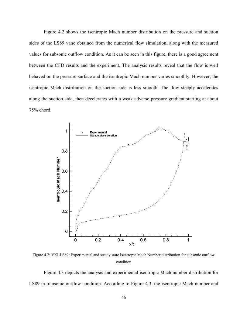
46

Figure 4.2 shows the isentropic Mach number distribution on the pressure and suction

sides of the LS89 vane obtained from the numerical flow simulation, along with the measured

values for subsonic outflow condition. As it can be seen in this figure, there is a good agreement

between the CFD results and the experiment. The analysis results reveal that the flow is well

behaved on the pressure surface and the isentropic Mach number varies smoothly. However, the

isentropic Mach distribution on the suction side is less smooth. The flow steeply accelerates

along the suction side, then decelerates with a weak adverse pressure gradient starting at about

75% chord.

Figure 4.2: VKI-LS89: Experimental and steady state Isentropic Mach Number distribution for subsonic outflow

condition

Figure 4.3 depicts the analysis and experimental isentropic Mach number distribution for

LS89 in transonic outflow condition. According to Figure 4.3, the isentropic Mach number and

47

hence the pressure varies smoothly on the pressure side similar to the lower exit Mach number

condition. However, the flow accelerates rapidly on the suction surface and a shock wave occurs

at about 85% chord which is followed by a high diffusion. There is a good agreement between

the experimental and analysis results on the pressure side. Small discrepancies are observed for

the Mach number on the suction surface near the shock region which might be due to laminar to

turbulent transition on the rear part of the suction side which occurs in the experiment and some

related unsteady effects [34].

Figure 4.3: VKI-LS89: Experimental and steady state Isentropic Mach Number distribution for transonic outflow

condition

The LS89 vane has been inversely redesigned for both operating points where the exit

Mach number is M2,is = 0.875 and M2,is = 1.02. In both cases, the first 6% and the last 5% of the

blade were run in analysis mode in order to ensure a physical closed blade shape. The L2-norm of

48

the grid velocity and the pressure difference were monitored as the convergence criteria for the

inverse design.

4.1.1 Redesigning VKI-LS89 in Subsonic Outflow Condition

In the subsonic outflow condition, the suction side pressure and tangential thickness are chosen

as the design variables. This is due to the fact that the flow is well behaved on the pressure side

and pressure does not require to be smoothed. Figure 4.4 shows the original, target and design

pressure on the suction side for subsonic outflow condition. As it can be seen in this figure, the

target pressure distribution is smoothed between 30% and 85% of the chord.

Figure 4.4: VKI-LS89: Original, target and design suction side pressure distribution for subsonic outflow

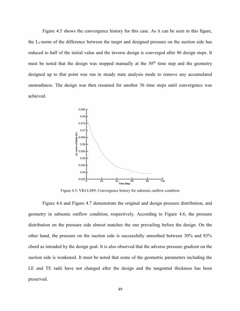
49

Figure 4.5 shows the convergence history for this case. As it can be seen in this figure,

the L2-norm of the difference between the target and designed pressure on the suction side has

reduced to half of the initial value and the inverse design is converged after 86 design steps. It

must be noted that the design was stopped manually at the 50th time step and the geometry

designed up to that point was run in steady state analysis mode to remove any accumulated

unsteadiness. The design was then resumed for another 36 time steps until convergence was

achieved.

Figure 4.5: VKI-LS89: Convergence history for subsonic outflow condition

Figure 4.6 and Figure 4.7 demonstrate the original and design pressure distribution, and

geometry in subsonic outflow condition, respectively. According to Figure 4.6, the pressure

distribution on the pressure side almost matches the one prevailing before the design. On the

other hand, the pressure on the suction side is successfully smoothed between 30% and 85%

chord as intended by the design goal. It is also observed that the adverse pressure gradient on the

suction side is weakened. It must be noted that some of the geometric parameters including the

LE and TE radii have not changed after the design and the tangential thickness has been

preserved.

Time Step

L2

-n

orm

of

De

lta

(P-)

0 20 40 60 80 1000.035

0.04

0.045

0.05

0.055

0.06

0.065

0.07

0.075

0.08

0.085

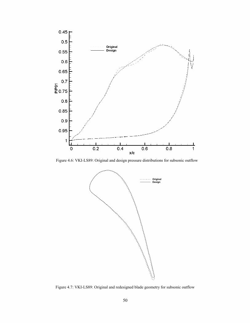
50

Figure 4.6: VKI-LS89: Original and design pressure distributions for subsonic outflow

Figure 4.7: VKI-LS89: Original and redesigned blade geometry for subsonic outflow

X

Y

0 0.02 0.04 0.06

-0.05

-0.04

-0.03

-0.02

-0.01

0

0.01

Original

Design

51

The performance characteristics of the original and redesigned blade are presented in

Table 4.3, where the pressure loss coefficient (휁) is defined as:

ζ = 1 −1 − (

𝑃2

𝑃02)

𝛾−1𝛾

1 − (𝑃2

𝑃01)

𝛾−1𝛾

(4.1)

Table 4.3: VKI-LS89: Aerodynamic Characteristics of the original and redesigned blade for subsonic outflow

Original Design

𝛇 % 5.40 5.21

Reduced Mass flow rate (�̇�𝒓𝒆𝒅) 0.2354 0.2366

According to Table 4.3, the pressure loss coefficient was reduced by 3.5% of the original

value while the reduced mass flow rate varied by 0.54%.

Figure 4.8: VKI-LS89: The analysis pressure distribution obtained in transonic outflow conditions using the

original, and design blade geometry obtained at subsonic outflow

52

The redesigned geometry in subsonic outflow condition, was also run in steady state

mode for transonic outflow condition to assess its performance. Figure 4.8 illustrates the original

analysis pressure distribution for M2,is= 1.02 (transonic outflow), and the analysis pressure

distribution on the redesigned blade geometry obtained in this section for the same outflow

conditions. According to this figure, the attained pressure on the suction side is much smoother

compared to the one corresponding to the original geometry; while the pressure side’s pressure

has almost remained unchanged. The pressure loss coefficient for this case is reduced by 5.4%

and the reduced mass flow rate varied by 0.82% compared to the original geometry as a result of

a smoother pressure distribution on the blade.

4.1.2 Redesigning VKI-LS89 in Transonic Outflow Condition

In the transonic outflow case, the suction and pressure side pressures are chosen as the design

variables. The reason for this choice rather than choosing suction side pressure and tangential

thickness is the fact that LS89 is a highly staggered blade with an extreme variation in normal

thickness from the LE to the TE. Consequently, preserving the tangential thickness (instead of

normal thickness) during the inverse design might lead to unphysical blade shapes, and in severe

cases the design crashes after a few time steps. On the other hand, in transonic outflow condition

the flow is much more sensitive to any changes in the blade geometry compared to the subsonic

flow; which results in a drastic change in the surface pressure. Furthermore, in this case there is a

shock wave on the rear part of the suction side causing a high pressure gradient. That’s another

reason why attempting to redesign the LS89 using the tangential thickness as one of the design

variables (like the subsonic case) was unsuccessful.

53

Figure 4.9 shows the original, target and design pressure distributions for VKI-LS89 in

transonic outflow. As it can be seen in this figure, the design objective is to smooth the pressure

on the suction side while preserving the same pressure distribution on the pressure side. Besides,

it is intended to lower the maximum Mach number on the suction side and weaken the shock

wave.

Figure 4.9: VKI-LS89: Original, target and design pressure distribution for transonic outflow

It is seen in Figure 4.9 that the target pressure on the suction side is almost achieved.

Also, the minimum pressure has increased further than the prescribed value resulting in a lower

peak Mach number and adverse pressure gradient which has benefited the blade in terms of total

pressure loss. However, the pressure on the pressure side has been slightly altered despite the

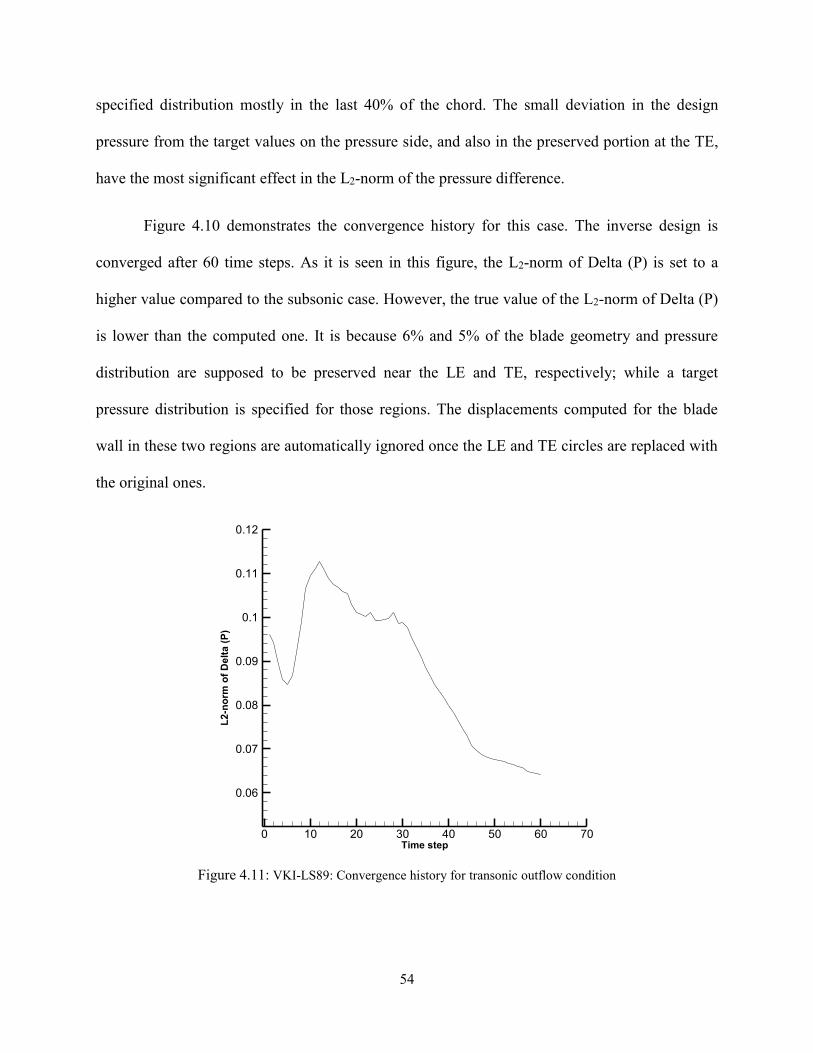
54

specified distribution mostly in the last 40% of the chord. The small deviation in the design

pressure from the target values on the pressure side, and also in the preserved portion at the TE,

have the most significant effect in the L2-norm of the pressure difference.

Figure 4.10 demonstrates the convergence history for this case. The inverse design is

converged after 60 time steps. As it is seen in this figure, the L2-norm of Delta (P) is set to a

higher value compared to the subsonic case. However, the true value of the L2-norm of Delta (P)

is lower than the computed one. It is because 6% and 5% of the blade geometry and pressure

distribution are supposed to be preserved near the LE and TE, respectively; while a target

pressure distribution is specified for those regions. The displacements computed for the blade

wall in these two regions are automatically ignored once the LE and TE circles are replaced with

the original ones.

Figure 4.11: VKI-LS89: Convergence history for transonic outflow condition

Time step

L2

-no

rmo

fD

elt

a(P

)

0 10 20 30 40 50 60 70

0.06

0.07

0.08

0.09

0.1

0.11

0.12

55

Figure 4.12: VKI-LS89: Original and redesigned blade geometry for transonic outflow

Figure 4.12 depicts the original and redesigned blade geometry. Unlike the subsonic

redesigned blade, the change in blade shape is almost unnoticed visually. The aerodynamic

characteristics of the original and redesigned LS89 are presented in Table 4.4. According to this

table, the pressure loss coefficient is reduced by 4% of its original value while the reduced mass

flow rate is matched up to 0.01%.

Table 4.4: VKI-LS89: Aerodynamic Characteristics of the original and redesigned blade for transonic outflow

Original Design

𝛇 % 5.75 5.52

Reduced Mass flow rate (�̇�𝒓𝒆𝒅) 0.23749 0.23751

X

Y

0 0.02 0.04 0.06

-0.05

-0.04

-0.03

-0.02

-0.01

0

0.01

Original

Design

56

4.2 E/CO-3 Compressor Stage Redesign

E/CO-3 is a single stage subsonic compressor. The geometric characteristics of the mid-span

section of this stage is listed in Table 4.5 [32].

Table 4.5: E/CO-3: Stage geometric characteristics

Rotor Stator

Number of Blades 41 73

Inlet Blade angle 57.79° 36.64°

Outlet Blade angle 43.03° -9.23°

Stagger angle 49° 14°

Spacing to Chord ratio 0.9 0.7

Reynolds Number 0.7×106 0.6×106

The mid-span section of this compressor has been previously analyzed in ANSYS-CFX

at three points on the design speed line (of 9,262.5 rpm) namely Maximum flow, Design point

and Near surge by Arbabi [30]. The details of the computational domain, flow solver and the

results validation can be found in [30]. It must be noted that the governing equations, turbulence

model, and the scheme used for turbulence numeric and advection terms are identical to the ones

applied in this work throughout analysis and redesign. Table 4.6 summarizes the analysis results

for E/CO-3 at maximum flow and near surge operating points [30].

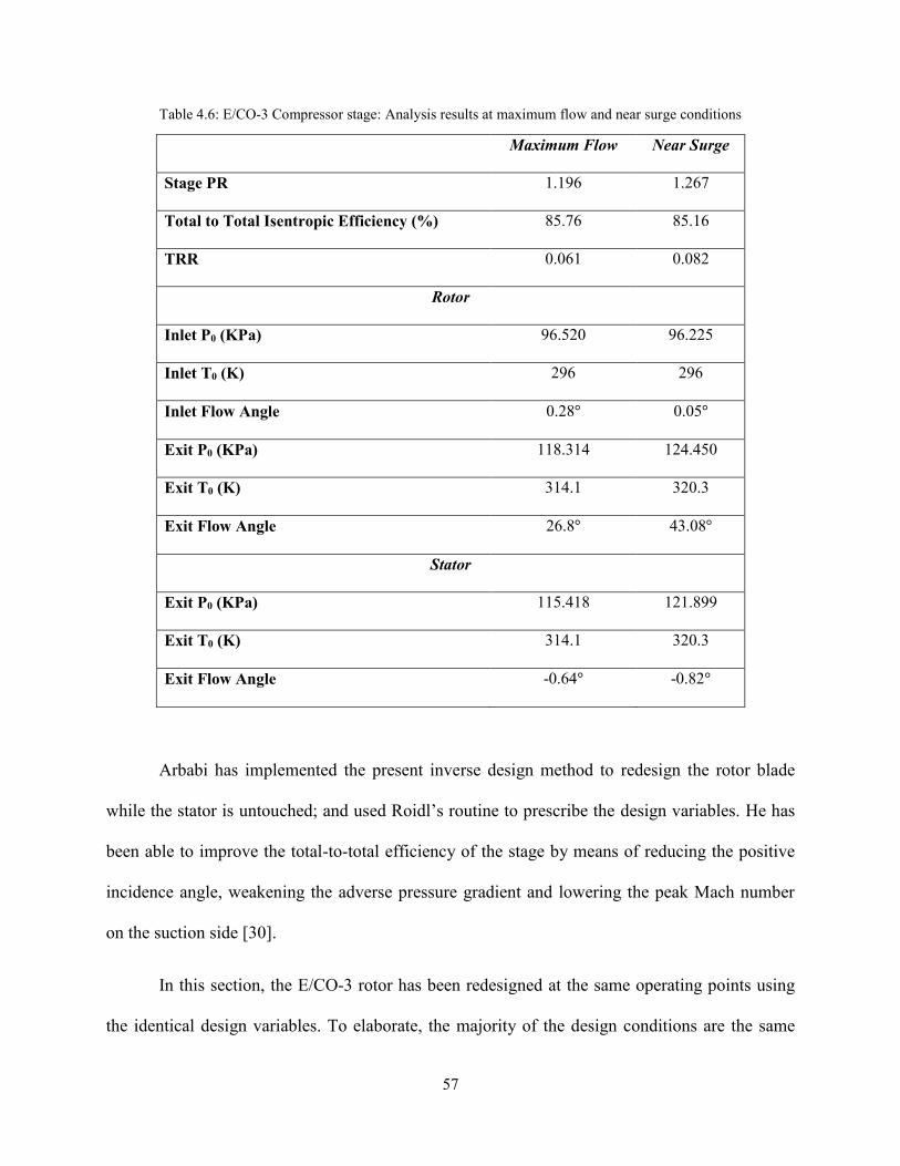
57

Table 4.6: E/CO-3 Compressor stage: Analysis results at maximum flow and near surge conditions

Maximum Flow Near Surge

Stage PR 1.196 1.267

Total to Total Isentropic Efficiency (%) 85.76 85.16

TRR 0.061 0.082

Rotor

Inlet P0 (KPa) 96.520 96.225

Inlet T0 (K) 296 296

Inlet Flow Angle 0.28° 0.05°

Exit P0 (KPa) 118.314 124.450

Exit T0 (K) 314.1 320.3

Exit Flow Angle 26.8° 43.08°

Stator

Exit P0 (KPa) 115.418 121.899

Exit T0 (K) 314.1 320.3

Exit Flow Angle -0.64° -0.82°

Arbabi has implemented the present inverse design method to redesign the rotor blade

while the stator is untouched; and used Roidl’s routine to prescribe the design variables. He has

been able to improve the total-to-total efficiency of the stage by means of reducing the positive

incidence angle, weakening the adverse pressure gradient and lowering the peak Mach number

on the suction side [30].

In this section, the E/CO-3 rotor has been redesigned at the same operating points using

the identical design variables. To elaborate, the majority of the design conditions are the same

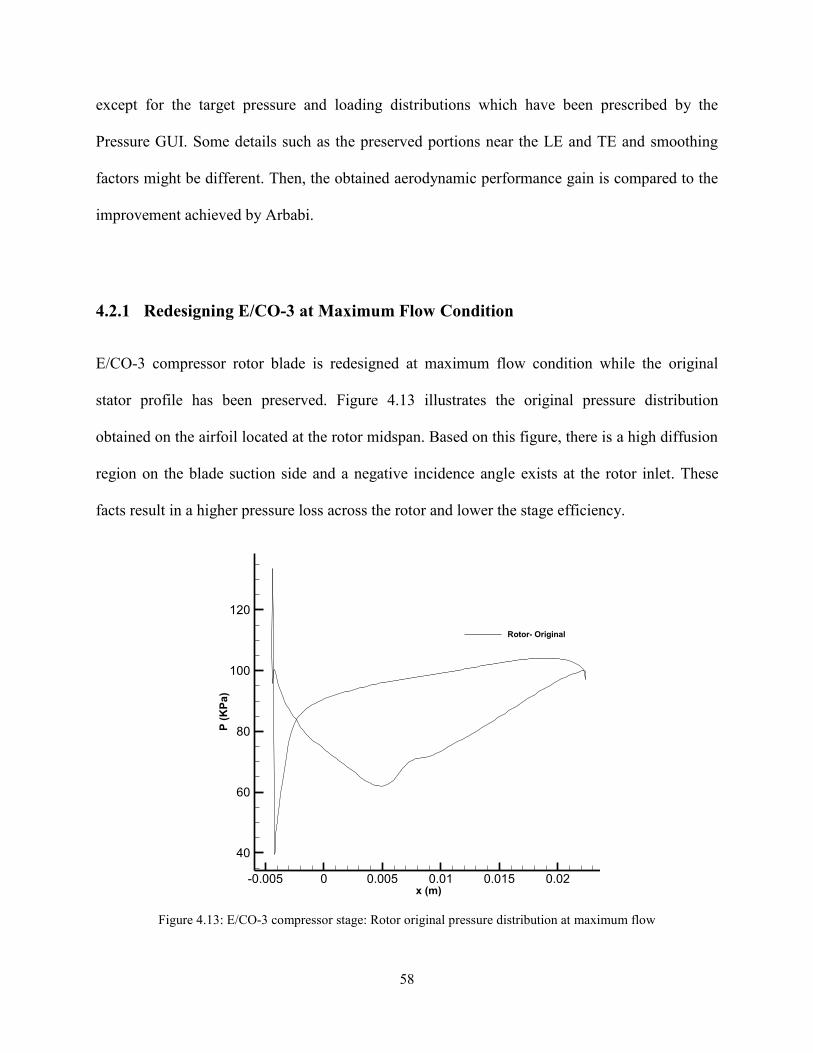
58

except for the target pressure and loading distributions which have been prescribed by the

Pressure GUI. Some details such as the preserved portions near the LE and TE and smoothing

factors might be different. Then, the obtained aerodynamic performance gain is compared to the

improvement achieved by Arbabi.

4.2.1 Redesigning E/CO-3 at Maximum Flow Condition

E/CO-3 compressor rotor blade is redesigned at maximum flow condition while the original

stator profile has been preserved. Figure 4.13 illustrates the original pressure distribution

obtained on the airfoil located at the rotor midspan. Based on this figure, there is a high diffusion

region on the blade suction side and a negative incidence angle exists at the rotor inlet. These

facts result in a higher pressure loss across the rotor and lower the stage efficiency.

Figure 4.13: E/CO-3 compressor stage: Rotor original pressure distribution at maximum flow

x (m)

P(K

Pa

)

-0.005 0 0.005 0.01 0.015 0.02

40

60

80

100

120

Rotor- Original

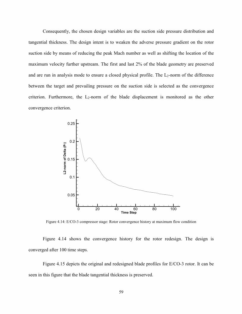
59

Consequently, the chosen design variables are the suction side pressure distribution and

tangential thickness. The design intent is to weaken the adverse pressure gradient on the rotor

suction side by means of reducing the peak Mach number as well as shifting the location of the

maximum velocity further upstream. The first and last 2% of the blade geometry are preserved

and are run in analysis mode to ensure a closed physical profile. The L2-norm of the difference

between the target and prevailing pressure on the suction side is selected as the convergence

criterion. Furthermore, the L2-norm of the blade displacement is monitored as the other

convergence criterion.

Figure 4.14: E/CO-3 compressor stage: Rotor convergence history at maximum flow condition

Figure 4.14 shows the convergence history for the rotor redesign. The design is

converged after 100 time steps.

Figure 4.15 depicts the original and redesigned blade profiles for E/CO-3 rotor. It can be

seen in this figure that the blade tangential thickness is preserved.

Time Step

L2

-no

rmo

fD

elt

a(P

-)

0 20 40 60 80 100

0.05

0.1

0.15

0.2

0.25

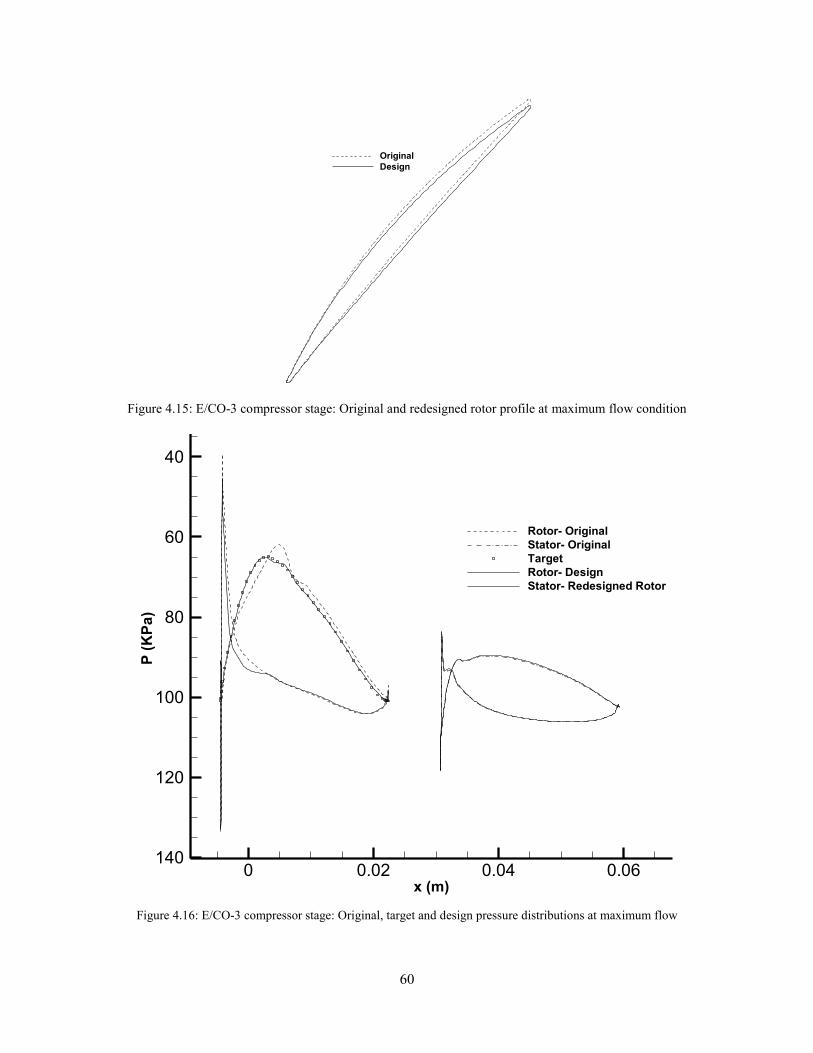
60

Figure 4.15: E/CO-3 compressor stage: Original and redesigned rotor profile at maximum flow condition

Figure 4.16: E/CO-3 compressor stage: Original, target and design pressure distributions at maximum flow

X

Y

0 0.01 0.02 0.03

-0.04

-0.035

-0.03

-0.025

-0.02

-0.015

-0.01

-0.005

Original

Design

x (m)

P(K

Pa

)

0 0.02 0.04 0.06

40

60

80

100

120

140

Rotor- Original

Stator- Original

Target

Rotor- Design

Stator- Redesigned Rotor

61

Figure 4.16 illustrates the original and design pressure distributions for both rotor and

stator, as well as the target pressure on the rotor suction side. As it can be seen in this figure, the

peak Mach number on the suction side is lowered significantly and the flow diffusion occurs

over a bigger region, hence reducing the adverse pressure gradient. On the other hand, the

pressure distribution on the pressure side has not changed significantly. Table 4.7 summarizes

the stage aerodynamic characteristics before and after redesigning the rotor, as well as the

obtained results in the previous redesign by Arbabi. According to this table, the compressor stage

total to total efficiency and pressure ratio have increased by 1.07% and 0.17% of the original

value in this work, respectively. These values confirm that the design intent is achieved and the

stage performance has been improved.

Table 4.7: E/CO-3 compressor stage: Original and redesigned Aerodynamic characteristics at maximum flow

Original Design Previous

Design1 [30] Previous

Design2 [30]

Efficiency (%) 85.76 86.68 86.32 86.42

Stage PR 1.196 1.198 1.198 1.197

TRR 0.0611 0.0611 0.0612 0.0610

Exit P0 (KPa) 115.41 115.64 115.6 115.5

Exit T0 (K) 314.10 314.09 314.12 314.10

Relative flow angle at Rotor Inlet 54.87° 54.88° 54.60° 54.69°

Relative flow angle at Rotor Exit 44.31° 44.01° 44.11° 44.26°

Relative Mach No. at Rotor Exit 0.635 0.638 0.637 0.636

62

4.2.2 Redesigning E/CO-3 at Near Surge Condition

E/CO-3 compressor rotor blade is redesigned at near surge condition while the original stator

profile has been preserved. The design variables are the blade tangential thickness and loading

(DP) distribution. The design intent is to lower the positive incidence and high diffusion at the

rotor inlet which increased the blade losses. The blade is redesigned using two different target

loading distributions to demonstrate that even the slightest changes in the design variables could

affect the final blade geometry and aerodynamic performance considerably. For both cases, the

first 2.5% of the LE and the last 2% of the TE is run in analysis mode.

Figure 4.17 and Figure 4.18 show the convergence history for both redesign cases. The

design is converged after 60 and 35 time steps for target 1 and target 2, respectively.

Figure 4.17: E/CO-3 compressor stage: Rotor convergence

history at near surge condition (Design 1)

Figure 4.18: E/CO-3 compressor stage: Rotor convergence

history at near surge condition (Design 2)

Figure 4.19 depicts the original and redesigned blade profiles using target 1 and target 2.

Figure 4.20 shows the original and target loadings, as well as the obtained design loading

Time Step

L2

-no

rmo

fd

elt

a(D

P)

0 5 10 15 20 25 30 35 40

0.05

0.1

0.15

0.2

0.25

63

distributions. Figure 4.21 demonstrates the original and design pressure distributions on both

suction and pressure sides of the blade. The original and redesigned stage aerodynamic

characteristics are also tabulated in Table 4.8.

Figure 4.19: E/CO-3 compressor stage: Original and redesigned rotor profile at near surge condition

As it can be seen in Figure 4.20 and Figure 4.21, the leading edge spike has been lowered

for both target loadings. This reveals that the positive incidence and high diffusion on the suction

side have been reduced. The decrease in the positive incidence has resulted in a lower pressure

loss across the rotor blade leading to an increase in the stage pressure ratio. According to

Table 4.8, this parameter is increased by 0.4% and 0.2% of the original value in Design 1 and

Design 2, respectively. Besides, both designs have resulted in a notable increase in the stage total

to total efficiency. This parameter is increased by 1.7% and 1.3% for target 1 and target 2,

respectively (Table 4.8).

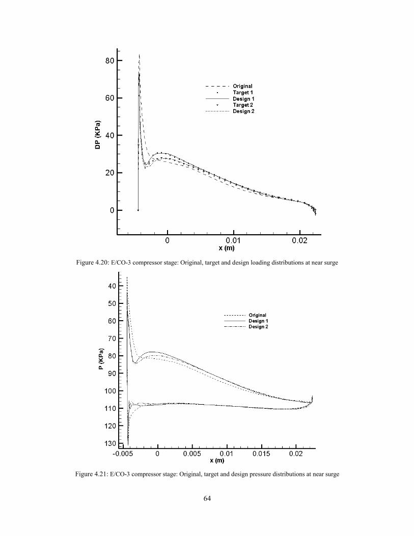
64

Figure 4.20: E/CO-3 compressor stage: Original, target and design loading distributions at near surge

Figure 4.21: E/CO-3 compressor stage: Original, target and design pressure distributions at near surge

65

Table 4.8: E/CO-3 compressor stage: Original and redesigned Aerodynamic characteristics at near surge

Original Design 1 Design 2 Previous

Design[30]

Efficiency (%) 85.16 86.86 86.48 87.07

Stage PR 1.267 1.272 1.270 1.271

TRR 0.0823 0.0819 0.0817 0.0816

Exit P0 (KPa) 121.899 122.381 122.151 122.3

Exit T0 (K) 320.29 320.25 320.16 320.14

Relative flow angle at Rotor Inlet 61.96° 61.07° 61.54° 61.24°

Relative flow angle at Rotor Exit 45.44° 44.86° 45.44° 45.24°

Relative Mach No. at Rotor Exit 0.477 0.484 0.480 0.482

4.2.3 E/CO-3 Compressor Stage Redesign Performance Gain over the Previous

Method

In this section, the obtained results in sections 4.2.1 and 4.2.2 are compared to the aerodynamic

performance gain achieved by Arbabi [30] in redesigning E/CO-3 compressor stage.

At maximum flow condition, Arbabi has redesigned the rotor blade using two different

set of design variables: suction side pressure distribution and tangential thickness, and loading

distribution and tangential thickness. The aerodynamic characteristics of the original airfoil and

the redesigned airfoils in the present and previous work at maximum flow condition is presented

in Table 4.7. The design case referred to as “Previous Design 1” corresponds to Arbabi’s first set

of design variables and “Previous Design 2” corresponds to his second set of design variables.

According to this table, Arbabi has been able to improve the stage total to total efficiency by

0.56% and 0.66% in the first and second redesign cases, respectively. Also, the stage pressure

66

ratio has been increased by 0.17% and 0.08% of the original PR in design 1 and design 2,

respectively.

In the current work, the suction side pressure distribution and tangential thickness are

chosen as the design variables at maximum flow condition. According to Table 4.7, the stage

efficiency is increased by 0.92% and the stage pressure ratio improved by 0.17% of the original

value. It is more valid to compare the results from the present design with the first design case in

Arbabi’s work due to the identical design variables. However, the achieved performance

improvement in the current work is greater than improvements accomplished by Arbabi in both

design cases.

At near surge condition, Arbabi has chosen the loading distribution and tangential

thickness as his design variables which is the same as the selected design variables in the present

work for this operating condition. The aerodynamic characteristics of the original airfoil and the

redesigned airfoils in the present and previous work at near surge condition are tabulated in

Table 4.8. According to this table, the best results in this work for the near surge redesign

correspond to the first design case with 1.7% and 0.4% improvement in the stage efficiency and

pressure ratio, respectively. Arbabi has been able to increase the stage total to total efficiency by

1.9% which is slightly higher than the attained value in the present work. This is due to the

significant reduction in the positive incidence angle at the rotor inlet which has led to the

decrease in the pressure loss across the stage. On the other hand, the stage pressure ratio has been

improved by 0.32% of the original value in Arbabi’s work which is slightly less than the

achieved PR in this work.

Comparing the aerodynamic performance gain obtained from the previous and current

redesigns, it can be concluded that the target design variable, namely pressure distribution has

67

been well tailored to achieve the design intent in the present work. This fact confirms the

influential role of the prescribed design variables and consequently, the Pressure GUI in

accomplishing better aerodynamic performance in 2D inverse shape design.

68

Chapter 5

5 Conclusion

5.1 Summary

B-Spline curves and surfaces have been employed for representing and modifying the blade

geometry and design variables. While B-spline curves have been used for interpolating the airfoil

geometry in the scope of this work, B-spline surface generation is applied in the extension of the

present 2D inverse shape design to 3D inverse design. Care has been taken to enhance the

geometry representation by studying the effect of various B-spline parameters such as point

clustering on the interpolation errors, and several examples of airfoil curve and blade surface

construction are provided.

Another contribution of the present work is the development of a robust and user-friendly

numerical tool for specifying the design variables based on B-splines. While there is a lack of

information in the open literature on numerical methods for prescribing the design variables for

inverse shape design despite of its importance, the current work provides a method for

generating 2D target pressure or pressure loading curves and 3D target pressure surfaces. The

multi-segment yet smooth and continuous nature of the B-splines served in providing a method

which enables designer to have local control on the generated pressure or loading curves. This

69

feature makes the designer capable of tailoring the design variables so as to account for all the

required aspects of aerodynamic design, which contributes to the successful implementation of

inverse shape design. The relatively small number of parameters required to represent even

complex profiles using B-splines makes them well-suited for interactive target generation.

The application of this novel method for the generation of the target design variables in

2D inverse shape design and its role in improving the aerodynamic performance is demonstrated

by several redesign cases where the performance of a transonic turbine vane and the rotor of a

compressor stage are improved under different flow conditions. The satisfaction of the design

intents and hence, the considerable performance gain is a direct result of the efficiency and

applicability of the developed method for prescribing the design variables.

Finally, the developed method could lend itself well to accomplish the design intents and

performance improvement in three-dimensional inverse shape design similar to two-dimensional

design.

5.2 Future Work

The success of using B-splines in the numerical representation and interpolation of the airfoil

shape and the design variables in 2D inverse shape design has been demonstrated in this work.

The next step is to extend the use of B-splines in representing (numerically) and interpolating the

blade surface as well as the design variables in inverse blade design in 3D flow, along the same

lines given in Appendix A and Appendix B.

70

Also, this work focused primarily on establishing a method and means for representing

and modifying design variables in 2D and 3D internal flow. The developed tool for describing

numerically the target or design variables, is not sufficient alone for a successful and efficient

turbomachinery design. It is recommended to begin a study on the choice of design variables,

which is based on flow physics, for prescribing target loading (or pressure) distributions which

could address the challenges faced by designers, especially in 3D inverse shape design where the

presence of various interdependent phenomena makes flow physics much more complicated.

71

References

[1] Lee Y-, Luo L, Bein TW. Direct method for optimization of a centrifugal compressor

vaneless diffuser. Journal of Turbomachinery. 2001;123(1):73-80.

[2] Pierret S, Van DB. Turbomachinery blade design using a Navier-Stokes solver and Artificial

Neural Network. Journal of Turbomachinery. 1999;121(2):326-32.

[3] Page JH, Hield P, Tucker PG. Inverse design of 3D multistage transonic fans at dual

operating points. Journal of Turbomachinery. 2014;136(4).

[4] Demeulenaere A, Leonard O, Van dB. A two-dimensional Navier-Stokes inverse solver for

compressor and turbine blade design. Proc Inst Mech Eng A: J Power Energy. 1997;211(4):299-

307.

[5] De Vito L, Van DB, Deconinck H. A novel two dimensional viscous inverse design method

for turbomachinery blading. Proceedings of the ASME TURBO EXPO 2002: Turbomachinery,

June 3, 2002 - June 6; 2002; Amsterdam, Netherlands: American Society of Mechanical

Engineers; 2002.

[6] Giles MB, Drela M. Two-dimensional transonic aerodynamic design method. AIAA J.

1987;25(9):1199-206.

[7] Zangeneh M. Inviscid-viscous interaction method for 3D inverse design of centrifugal

impellers. ASME 1993 International Gas Turbine and Aeroengine Congress and Exposition, GT

1993, May 24, 1993 - May 27; 1993; Cincinnati, OH, United states: American Society of

Mechanical Engineers; 1993.

[8] Demeulenaere A, Van DB. Three-dimensional inverse method for turbomachinery blading

design. ASME 1996 International Gas Turbine and Aeroengine Congress and Exhibition, GT

1996, June 10, 1996 - June 13; 1996; Birmingham, United kingdom: Web Portal ASME

(American Society of Mechanical Engineers); 1996.

[9] Pascoa JC, Mendes AC, Gato LMC. A fast iterative inverse method for turbomachinery blade

design. Mech Res Commun. 2009 07;36(5):630-7.

[10] Mileshin VI, Orekhov IK, Shchipin SK, Startsev AN. New 3D inverse Navier-Stokes based

method used to design turbomachinery blade rows. 2004 ASME Heat Transfer/Fluids

Engineering Summer Conference, HT/FED 2004, July 11, 2004 - July 15; 2004; Charlotte, NC,

United states: American Society of Mechanical Engineers; 2004.

[11] Daneshkhah K, Ghaly W. Aerodynamic inverse design for viscous flow in turbomachinery

blading. J Propul Power. 2007 07;23(4):814-20.

72

[12] Daneshkhah K, Ghaly W. An inverse design method for viscous flow in turbomachinery

blading using a wall virtual movement. Inverse Problems in Science and Engineering.

2009;17(3):381-97.

[13] Arbabi A, Ghaly W. Inverse design of turbine and compressor stages using a commercial

CFD program. ASME Turbo Expo 2013: Turbine Technical Conference and Exposition, GT

2013, June 3, 2013 - June 7; 2013; San Antonio, Tx, United states: American Society of

Mechanical Engineers; 2013.

[14] Nicoud D, Le Bloa C, Jacquotte O. Finite element inverse method for the design of

turbomachinery blades. International Gas Turbine and Aeroengine Congress and Exposition,

June 3, 1991 - June 6; 1991; Orlando, FL, USA: Publ by ASME; 1991.

[15] Zannetti L, Pandolfi M. INVERSE DESIGN TECHNIQUE FOR CASCADES. 1984.

[16] Leonard O, Van dB. Design method for subsonic and transonic cascade with prescribed

Mach number distribution. Journal of Turbomachinery. 1992;114(3):553-60.

[17] Ahmadi M, Ghaly WS. Aerodynamic inverse design of turbomachinery cascades using a

finite volume method on unstructured meshes. Inverse Problems in Engineering. 1998 09/01;

2015/06;6(4):281-98.

[18] Medd AJ, Dang TQ, Larosiliere LM. 3D inverse design loading strategy for transonic axial

compressor blading. 2003 ASME Turbo Expo, June 16, 2003 - June 19; 2003; Atlanta, GA,

United states: American Society of Mechanical Engineers; 2003.

[19] van E, J.A. Numerical optimization of target pressure distributions for subsonic and

transonic airfoil design. Specialists' Meeting of the Fluid Dynamics; May 22 - 23 1989; Loen,

Norw: Publ by AGARD; 1989.

[20] Jiao-Zan Li, Zheng-Hong Gao. Inverse Design Method of Airfoil Embedded Optimization

of Pressure Distribution. Third International Conference on Information and Computing Science

(ICIC 2010); 4-6 June 2010; Los Alamitos, CA, USA: IEEE Computer Society; 2010.

[21] Liu Y, Ma D. Inverse Design of Airfoils Using Target Pressure Optimization. Advanced

Materials Research. 2013;694-697:3183-8.

[22] Obayashi S, Takanashi S. Genetic optimization of target pressure distributions for inverse

design methods. AIAA J. 1996 05/01; 2015/06;34(5):881-6.

[23] Roidl B, Ghaly W. Dual point redesign of axial turbines using a viscous inverse design

method. 2009 ASME Turbo Expo, June 8, 2009 - June 12; 2009; Orlando, FL, United states:

American Society of Mechanical Engineers; 2009.

[24] Ramamurthy R, Ghaly W. Dual point redesign of an axial compressor airfoil using a viscous

inverse design method. ASME Turbo Expo 2010: Power for Land, Sea, and Air, GT 2010, June

73

14, 2010 - June 18; 2010; Glasgow, United kingdom: American Society of Mechanical

Engineers; 2010.

[25] Roidl B. Aerodynamic Inverse Design of Multistage Turbomachinery Blading [dissertation].

Department of Mechanical and Industrial Engineering: Concordia University; 2008.

[26] ANSYS Inc. ANSYS CFX Release Notes for 14.5. October 2012.

[27] Daneshkhah K. Aerodynamic inverse design of turbomachinery blading in two-dimensional

viscous flow [dissertation]. Concordia University, Department of Mechanical and Industrial

Engineering; 2007.

[28] Thompkins Jr. WT, Siu ST. INVERSE OR DESIGN CALCULATIONS FOR

NONPOTENTIAL FLOW IN TURBOMACHINERY BLADE PASSAGES. Journal of

engineering for power. 1982;104(2):281-5.

[29] Siu ST, Thompkins Jr. WT. DESIGN CALCULATION PROCEDURE FOR SHOCK-

FREE OR STRONG PASSAGE SHOCK TURBOMACHINERY CASCADES. 27th

International Gas Turbine Conference and Exhibit. London, Engl: ASME; 1982.

[30] Arbabi A. Aerodynamic inverse shape design of compressor and turbine stages using

ANSYS-CFX [dissertation]. Concordia University, Department of Mechanical and Industrial

Engineering; 2012.

[31] Mengistu T, Ghaly W. A Geometric Representation of Turbomachinery Cascades Using

NURBS. AIAA paper No. 2002-0318. 2002.

[32] Fottner L. Test Cases for Computation of Internal Flows in Aero Engine Components.

Propulsion and Energetics Panel; 1990.

[33] Arts T, de Rouvroit L, Rutherford A. Aero-Thermal investigation of a highly loaded

transonic linear turbine guide vane cascade. Technical Note 174. Von Karman Institute for Fluid

Dynamics; 1990.

[34] Daneshkhah K, Ghaly W. Redesign of a highly loaded transonic turbine nozzle blade using

a new viscous inverse design method. ASME Turbo Expo 2007 Power for Land, Sea and Air;

Montreal, Canada. ; 2007.

[35] Piegl L, Tiller W. The Nurbs Book. 2nd ed. Germany: Springer; 1997.

[36] Dang T, Damle S, Qiu X. Euler-Based Inverse Method for Turbomachine Blades, Part 2:

Three-Dimensional Flows. AIAA Journal. 2000;38(11):2007-13.

74

APPENDIX A

A B-Spline Curve and Surface Interpolation

As it was stated in chapter 3, B-splines have been employed for curve interpolation in the scope

of this work and examples of their application in representing airfoils and the corresponding

interpolation errors were presented. It was also mentioned in section 1.2 that one of the tasks in

the present work is to develop a robust and precise three-dimensional representation for both the

blade geometry and design variables. This representation is implemented in the extension of the

current two-dimensional inverse technique to three-dimensional inverse shape design. In this

appendix, B-spline curve preliminaries and one of the B-spline surface generation methods

called “Global Surface Interpolation” are discussed in details. Also, one of the applications of the

aforementioned method which is representing the three-dimensional blade geometry will be

shown by examples.

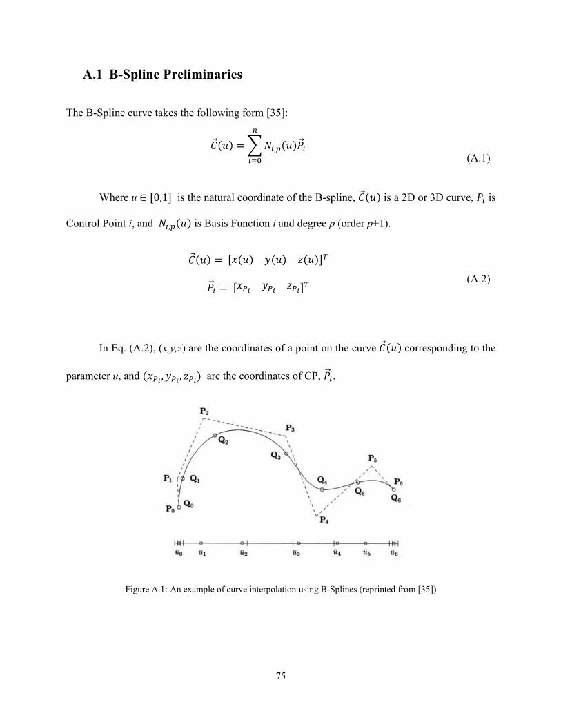
75

A.1 B-Spline Preliminaries

The B-Spline curve takes the following form [35]:

𝐶(𝑢) = ∑ 𝑁𝑖,𝑝(𝑢)�⃗⃗�𝑖

𝑛

𝑖=0

(A.1)

Where u ∈ [0,1] is the natural coordinate of the B-spline, 𝐶(𝑢) is a 2D or 3D curve, 𝑃𝑖 is

Control Point i, and 𝑁𝑖,𝑝(𝑢) is Basis Function i and degree p (order p+1).

𝐶(𝑢) = [𝑥(𝑢) 𝑦(𝑢) 𝑧(𝑢)]𝑇

�⃗⃗�𝑖 = [𝑥𝑃𝑖𝑦𝑃𝑖

𝑧𝑃𝑖]𝑇 (A.2)

In Eq. (A.2), (x,y,z) are the coordinates of a point on the curve 𝐶(𝑢) corresponding to the

parameter u, and (𝑥𝑃𝑖, 𝑦𝑃𝑖

, 𝑧𝑃𝑖) are the coordinates of CP, �⃗⃗�𝑖.

Figure A.1: An example of curve interpolation using B-Splines (reprinted from [35])

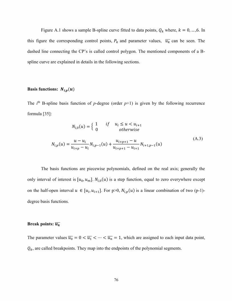
76

Figure A.1 shows a sample B-spline curve fitted to data points, 𝑄𝑘 where, 𝑘 = 0, … ,6. In

this figure the corresponding control points, 𝑃𝑘 and parameter values, 𝑢𝑘̅̅ ̅ can be seen. The

dashed line connecting the CP’s is called control polygon. The mentioned components of a B-

spline curve are explained in details in the following sections.

Basis functions: 𝑵𝒊,𝒑(𝒖)

The ith B-spline basis function of p-degree (order p+1) is given by the following recurrence

formula [35]:

𝑁𝑖,0(𝑢) = { 1 𝑖𝑓 𝑢𝑖 ≤ 𝑢 < 𝑢𝑖+1

0 𝑜𝑡ℎ𝑒𝑟𝑤𝑖𝑠𝑒

𝑁𝑖,𝑝(𝑢) =𝑢 − 𝑢𝑖

𝑢𝑖+𝑝 − 𝑢𝑖𝑁𝑖,𝑝−1(𝑢) +

𝑢𝑖+𝑝+1 − 𝑢

𝑢𝑖+𝑝+1 − 𝑢𝑖+1𝑁𝑖+1,𝑝−1(𝑢)

(A.3)

The basis functions are piecewise polynomials, defined on the real axis; generally the

only interval of interest is [𝑢0, 𝑢𝑚]. 𝑁𝑖,0(𝑢) is a step function, equal to zero everywhere except

on the half-open interval 𝑢 ∈ [𝑢𝑖, 𝑢𝑖+1]. For p>0, 𝑁𝑖,𝑝(𝑢) is a linear combination of two (p-1)-

degree basis functions.

Break points: 𝒖𝒌̅̅̅̅

The parameter values 𝑢0̅̅ ̅ = 0 < 𝑢1̅̅ ̅ < ⋯ < 𝑢𝑛̅̅ ̅ = 1, which are assigned to each input data point,

𝑄𝑘, are called breakpoints. They map into the endpoints of the polynomial segments.

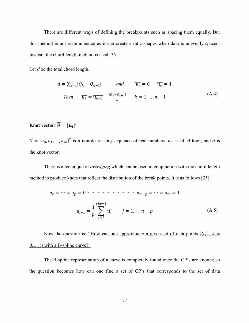
77

There are different ways of defining the breakpoints such as spacing them equally. But

this method is not recommended as it can create erratic shapes when data is unevenly spaced.

Instead, the chord length method is used [35].

Let d be the total chord length.

𝑑 = ∑ |𝑄𝑘 − 𝑄𝑘−1|𝑛𝑘=1 and 𝑢0̅̅ ̅̅ = 0 𝑢𝑛̅̅ ̅ = 1

Then 𝑢𝑘̅̅ ̅ = 𝑢𝑘−1̅̅ ̅̅ ̅̅ +|𝑄𝑘−𝑄𝑘−1|

𝑑 𝑘 = 1, … , 𝑛 − 1

(A.4)

Knot vector: �⃗⃗⃗� = [𝒖𝒊]𝑻

�⃗⃗⃗� = {𝑢0, 𝑢1, … , 𝑢𝑚}𝑇 is a non-decreasing sequence of real numbers. 𝑢𝑖 is called knot, and �⃗⃗⃗� is

the knot vector.

There is a technique of averaging which can be used in conjunction with the chord length

method to produce knots that reflect the distribution of the break points. It is as follows [35].

𝑢0 = ⋯ = 𝑢𝑝 = 0 ⋯ ⋯ ⋯ ⋯ ⋯ ⋯ ⋯ ⋯ ⋯ ⋯ 𝑢𝑚−𝑝 = ⋯ = 𝑢𝑚 = 1

𝑢𝑗+𝑝 =1

𝑝∑ 𝑢𝑖

𝑗+𝑝−1

𝑖=𝑗

𝑗 = 1, … , 𝑛 − 𝑝

(A.5)

Now the question is: “How can one approximate a given set of data points {𝑄𝑘}, 𝑘 =

0, … , 𝑛 with a B-spline curve?”

The B-spline representation of a curve is completely found once the CP’s are known; so

the question becomes how can one find a set of CP’s that corresponds to the set of data

78

{𝑄𝑘} 𝑤ℎ𝑒𝑟𝑒 𝑘 = 0, … , 𝑛, using a pth-degree B-spline curve? In fact, the following (n+1) × (n+1)

system of linear equations can be set up; where the control points, Pi are the unknowns:

𝑄𝑘 = 𝐶(𝑢𝑘̅̅ ̅) = ∑ 𝑁𝑖,𝑝(𝑢𝑘̅̅ ̅)𝑃𝑖

𝑛

𝑖=0

(A.6)

Where 𝐶(𝑢𝑘̅̅ ̅) is the interpolated curve which consists of n segments each of which is a

polynomial of pth-degree.

In order to solve for the unknown CP’s in Eq. (A.6), one needs to determine the

breakpoints 𝑢𝑘̅̅ ̅ and the corresponding knot vector �⃗⃗⃗� using Eq. (A.4) and (A.5), respectively.

Then, basis functions 𝑁𝑖,𝑝(𝑢𝑘̅̅ ̅) can be computed using Eq. (A.3) and the CP’s are obtained at the

data points.

A.2 B-spline Surface Interpolation

“Global Surface Interpolation” is a method based on B-splines for constructing surfaces. This

method inherits the principal features of B-spline curves which makes it robust and reliable. The

procedure to fit a surface through a number of data points using GSI is as follows.

Assume a set of (𝑛 + 1) × (𝑚 + 1) data points {𝑄𝑘,𝑙}, where 𝑘 = 0, … , 𝑛 and 𝑙 =

0, … , 𝑚 is given. {𝑄𝑘,𝑙} is typically a set of curves as shown in Figure A.2 which are called

section curves and can be planar or three-dimensional. The section curves are defined in the 𝑢

79

direction, and the blend direction is the 𝑣 (which is also referred to as longitudinal direction). A

non-rational (p,q)th-degree B-spline surface fitted to these points takes the following form.

𝑄𝑘,𝑙 = 𝑆(𝑢𝑘̅̅ ̅, 𝑣�̅�) = ∑ ∑ 𝑁𝑖,𝑝

𝑚

𝑗=0

𝑛

𝑖=0

(𝑢𝑘̅̅ ̅) 𝑁𝑗,𝑞(𝑣�̅�)𝑃𝑖,𝑗 (A.7)

The only unknown in this system of linear equations is the surface CP’s, 𝑃𝑖,𝑗 which needs

to be found to generate the B-spline surface.

Figure A.2: Sample of a number of section curves

The first step is to compute the parameter values, �̅�𝑘𝑙 for each cross sectional curve (𝑙 =

0, … , 𝑚) based on Eq. (A.4). Then, each �̅�𝑘 is computed by averaging across all �̅�𝑘𝑙 , 𝑙 = 0, … , 𝑚,

that is:

�̅�𝑘 =1

𝑚 + 1∑ �̅�𝑘

𝑙

𝑚

𝑙=0

𝑘 = 0, … , 𝑛 (A.8)

Y

X

Z

80

Once the common parameter values �̅�𝑘 are computed, knot vector U is calculated using

Eq. (A.5). This will be the common knot vector for all the section curves and will be used

throughout the calculations. It needs to be mentioned that �̅�𝑙 and V are calculated similarly.

The final step after the computation of the breakpoints and knot vectors is the calculation

of the surface control points. Eq. (A.7) represents (𝑛 + 1) × (𝑚 + 1) linear equations and the

unknowns are 𝑃𝑖,𝑗. As 𝑆(𝑢𝑘̅̅ ̅, 𝑣�̅�) is a tensor product surface, 𝑃𝑖,𝑗 can be computed more easily as a

sequence of curve interpolations. The following two relations demonstrate this sequence.

𝑄𝑘,𝑙 = ∑ 𝑁𝑖,𝑝(�̅�𝑘)

𝑛

𝑖=0

(∑ 𝑁𝑗,𝑞(�̅�𝑙) 𝑃𝑖,𝑗

𝑚

𝑗=0

) = ∑ 𝑁𝑖,𝑝(�̅�𝑘)

𝑛

𝑖=0

𝑅𝑖,𝑙 (A.9)

Where

𝑅𝑖,𝑙 = ∑ 𝑁𝑗,𝑞(�̅�𝑙) 𝑃𝑖,𝑗

𝑚

𝑗=0

(A.10)

𝑅𝑖,𝑙 in relation A.10 are the CP’s of the isoparametric curve on 𝑆(𝑢, 𝑣) at fixed 𝑣 = �̅�𝑙.

By fixing 𝑖 and letting 𝑙 vary, curve interpolation is done on the CP’s 𝑅𝑖,0, … , 𝑅𝑖,𝑚 and the

resulting surface CP’s 𝑃𝑖,0, … , 𝑃𝑖,𝑚 will be obtained. This process must be repeated 𝑛 + 1 times

to get all the control points 𝑃𝑖,𝑗.

81

The application of this method to generate three-dimensional blade surfaces is shown in

the next figures. Figure A.3 shows Rotor 37 which is constructed by GSI method using 8 section

curves in the spanwise direction.

Figure A.3: Rotor 37 blade surface interpolated by GSI method

Figure A.4 illustrates Stator 67 blade surface which is generated by GSI. Also, Figure A.5

shows two views of Rotor 67 constructed by the same method.

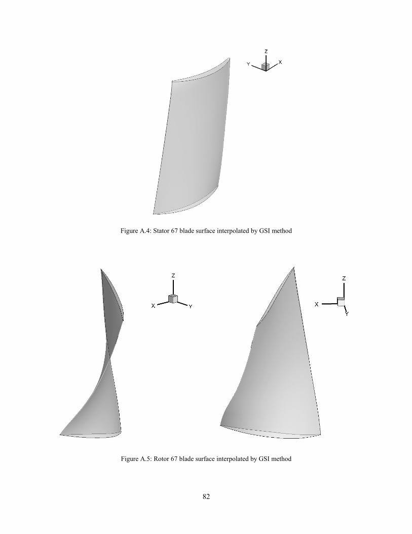
82

Figure A.4: Stator 67 blade surface interpolated by GSI method

Figure A.5: Rotor 67 blade surface interpolated by GSI method

83

APPENDIX B

B The Pressure GUI

In this Appendix, the developed Graphical User Interface (GUI) which is used for specification

of a target pressure (or loading) distribution is explained in detail. As it was stated in

section 3.2.2, this graphical interface is developed using MATLAB and works based on B-Spline

curves and surfaces. The details of the B-spline curve and surface generation can be found in

Appendix A.

The GUI can be used for two purposes: generating loading (or pressure) curves, and

creating loading (or pressure) surfaces. For simplicity, only the term “loading” is used

throughout this chapter. While a target loading curve is required as one of the inputs for two-

dimensional inverse design of an airfoil, a target loading surface is needed to inversely design a

three-dimensional blade.

Figure B.1 shows the general layout of the Pressure GUI once it is opened. As it can be

seen in this figure, the layout contains a toolbar and drop-down menu, several push buttons, and

two plots. Some of the push buttons are deactivated and will be only activated once certain

options are selected by the user. The function of each of the GUI components is briefly stated as

follows:

84

Figure B.1: General layout of Pressure GUI

“Open” Button

It opens the input file. The input must be an ASCII file. The data format is shown in Figure B.2.

The first line represents the number of input curves followed by the number of points on each

curve on the next lines, respectively. Then, the axial coordinates, corresponding loading, and

radial coordinates of each curve must be included.

Figure B.2: GUI input data format

85

Loading Plot

The axes on the left hand-side is used for plotting the original individual loading curves and

manipulating pre-defined CP’s to generate a target loading curve.

Meridional View of the Grid Lines

The right hand-side axes illustrate the meridional view of the input grid lines (mesh plot) and can

be seen in Figure B.3. This plot is mostly useful when user needs to specify a target loading for

several 2D sections along the span. It helps user to choose appropriate span-wise sections in

terms of radial spacing for the design. The total number of span-wise grid lines (or 2D sections)

is shown next to the plot.

Figure B.3: Sample of the meridional view of the input grid lines

86

“Select Grid Line” Input Box

This input box is to select the loading curve corresponding to the desired 2D section which is

meant to be redesigned. The input must be an integer smaller than or equal to the total number of

grid lines. The default value is 1. Once a number is entered into this box, the corresponding span-

wise location is highlighted in the Meridional view plot and the loading curve is plotted. Figure

B.3 demonstrates an example.

“Select Design Option” Drop-down Menu

This drop-down menu is used to select the design option. There are two options to choose from:

Design a few grid lines, and Design all the grid lines. The first option must be selected when the

output is required to be one or more than one loading curve(s). The second option must be

chosen when the output is required to be a loading surface.

Figure B.4: Sample of an original loading curve and generated target loading using Pressure GUI

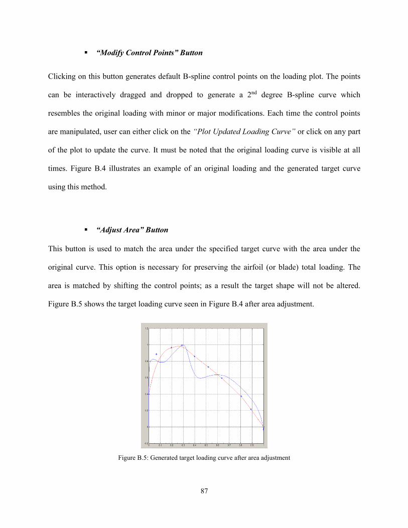
87

“Modify Control Points” Button

Clicking on this button generates default B-spline control points on the loading plot. The points

can be interactively dragged and dropped to generate a 2nd degree B-spline curve which

resembles the original loading with minor or major modifications. Each time the control points

are manipulated, user can either click on the “Plot Updated Loading Curve” or click on any part

of the plot to update the curve. It must be noted that the original loading curve is visible at all

times. Figure B.4 illustrates an example of an original loading and the generated target curve

using this method.

“Adjust Area” Button

This button is used to match the area under the specified target curve with the area under the

original curve. This option is necessary for preserving the airfoil (or blade) total loading. The

area is matched by shifting the control points; as a result the target shape will not be altered.

Figure B.5 shows the target loading curve seen in Figure B.4 after area adjustment.

Figure B.5: Generated target loading curve after area adjustment

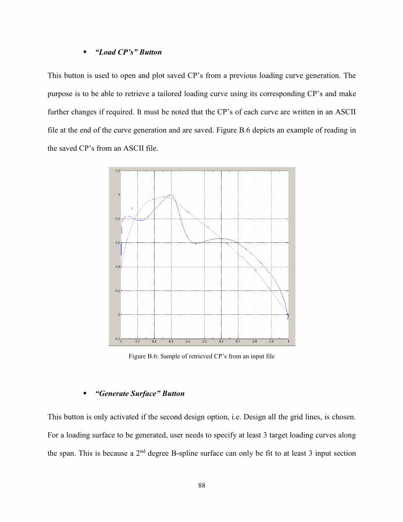
88

“Load CP’s” Button

This button is used to open and plot saved CP’s from a previous loading curve generation. The

purpose is to be able to retrieve a tailored loading curve using its corresponding CP’s and make

further changes if required. It must be noted that the CP’s of each curve are written in an ASCII

file at the end of the curve generation and are saved. Figure B.6 depicts an example of reading in

the saved CP’s from an ASCII file.

Figure B.6: Sample of retrieved CP’s from an input file

“Generate Surface” Button

This button is only activated if the second design option, i.e. Design all the grid lines, is chosen.

For a loading surface to be generated, user needs to specify at least 3 target loading curves along

the span. This is because a 2nd degree B-spline surface can only be fit to at least 3 input section

89

curves. The fitted surface is then plotted in a new window. More details will be provided in

section B.2.

“Clear” Button

This buttons clears all the plots, and input data.

“Write” Button

This push button is used to save the prescribed loading curves (and/or surface), and

corresponding CP’s. The files are written in the same format as the input.

In the next two sections, target loading curve and surface generation is explained in detail.

B.1 Target Loading Curve Generation

In order to create a single target loading curve, the original loading must be read into the GUI

using “Open” button. It is advised to use normalized values for the loading as well as axial

coordinates. The curve is automatically shown in the loading plot area. The next step is to choose

the design option from the drop-down menu. In this situation, “Design a few grid lines” must be

chosen. Once this option is selected, all the push buttons except for “Generate Surface” button

will be activated.

To start manipulating the curve, click on “Modify Control Points” to generate the pre-

defined control points on the plot. The number of CP’s used for curve fitting is set to be 8 by

90

default. However, it is possible for the user to increase or decrease this number to any desirable

value (greater than or equal to 3). This will provide the user with the opportunity to have more or

less control over the curve shape. The CP’s can be moved in any direction by the mouse;

however, the first and last CP’s are restricted to move in the y-direction to prevent any changes

in the axial chord length. As CP’s are moved, the fitted curve is constantly updated accordingly.

It goes without saying that the fitted curve will not necessarily pass through the CP’s.

Once the user is satisfied with the generated target curve, the area under the loading curve

can be matched by the area under the original curve to prevent changes in the blade loading.

“Adjust Area” button performs this area adjustment. In this case, the area under the original and

target curves are computed and the area ratio is obtained. This value is used to shift the CP’s so

as to match the area under the target curve with the original one. This process is repeated until a

certain tolerance is achieved. Once the area adjusted curve is plotted, the user has the possibility

to manipulate CP’s again if he/she is not satisfied with the final curve.

This procedure can take place for more than one curve at the same time; i.e. when the

user needs to define target loadings for more than one 2D span-wise sections on a 3D blade. This

will provide the designer with the opportunity to specify target loading curves for different 2D

sections while having the possibility to switch between loadings curves to tailor them

accordingly. For this purpose, one needs to input all the loading curves in one ASCII file as

mentioned in the previous section and go through each curve by selecting the span-wise section

index in the “Select grid line” box. Any time the user modifies a curve, the updated curve and

corresponding CP’s are saved and will be retrieved once the same curve is selected again for

further modifications.

91

B.2 Target Loading Surface Generation

Methods for three-dimensional inverse design of turbomachinery blades have been developed by

researchers such as Demeulenaere et al. [8], and Dang et al. [36]. On the other hand, the

developed 2D inverse design method discussed in this work is to be extended to three-

dimensional design. Regardless of the methodology, in any aerodynamic inverse design process

the first step for the designer is to tailor the design variables in certain ways to accomplish goals

such as enforcing a span-wise gradient, weakening or repositioning a shock wave, etc. In such

cases, the specification of local variables which would result in a global optimum is difficult.

This is specially challenging in the presence of strong three-dimensional effects such as tip and

hub clearance, which could change the flow field immediately. It also goes without saying that

for such cases, it is not desirable to have to specify every detail for the target along the whole

blade.

Despite all these concerns and the fact that several inverse design methodologies are

available and clearly elaborated in previous studies, very little is published about strategies and

methods for prescribing the design variables. The present work addresses this problem by using a

reliable B-spline interpolant for generating target design variables for three-dimensional blades.

For this purpose, the developed Pressure GUI which already provides user with the opportunity

to create multiple loading curves is used to generate surfaces from those input curves along the

span which would satisfy requirements in both streamwise and spanwise directions. As the

curves are interpolated using B-splines, the same tool is employed for surface construction. The

details of B-spline surface interpolation is explained in Appendix A.

92

As the imposed design variable in several previous works and the current study is either

the blade pressure or loading distribution, the developed Pressure GUI is customized for

generating pressure and loading surfaces. However, it might be used for specification of other

design variables such as Mach number by making minor modifications.

The interpolated loading surface by the Pressure GUI, inherits all the features

corresponding to the specified loadings by the designer and provides compatible smooth target

loadings for the intermediate sections which have not been directly tailored by the designer. This

will facilitate the designer’s job considerably.

In order to create a loading surface using the Pressure GUI, at least three target loading

curves must be prescribed in the spanwise direction because the degree of the interpolated B-

spline surface is 2 in this direction. For simplicity, the sections for which a target loading is

specified will be referred to as “Design sections”. The hub and tip must be necessarily included

in the design sections to satisfy boundary conditions for the B-spline interpolant. The number

and positioning of the other design sections is based on the design intents as well as controlling

the gradients in the spanwise direction. Special care has been taken to ensure a smooth transition

between the design sections and prevent generation of unphysical loading surfaces. Likewise, the

area under the loading surface is automatically matched with the original one to enforce the

blade original total work.

The steps for creating a loading surface begins with specifying a number of target loading

curves in the spanwise direction. This procedure was explained in the previous section. The only

difference is in the selection of the design option from the drop-down menu. In this case,

“Design all the grid lines” must be chosen which will activate the “Generate Surface” push

button. Besides, user is not required to adjust the area under the curve by pushing the “Adjust

93

Area” button, since this job is automatically done after surface fitting. Once specifying target

loadings for all the design sections is over, the user must press “Generate Surface” button to

interpolate a surface to the defined loading curves. Then, the interpolated loading surface before

and after area adjustment will be shown in two separate windows, enabling user to evaluate the

prescribed target. If the user is satisfied with the generated loading surface, the results can be

written out; otherwise, further changes may be made to the section curves and the procedure is

repeated. The written output is an ASCII file which contains the discrete target loading values for

all the individual axial and meridional locations in the original input file. Figure B.7 shows a

sample loading surface which is generated using the Pressure GUI.

Figure B.7: Interpolated loading surface using specified target loading at selected spanwise sections