Optimizing Dynamic Range for Distortion Measurements

Keysight Technologies Performance Spectrum Analyzer SeriesOptimizing Dynamic Range for Distortion Measurements

Application Note

https://www.TestWorld.com

Its wide dynamic range makes the spectrum analyzer the test instrument of choice for measuring

harmonic distortion, intermodulation distortion, adjacent channel power ratio, spurious-free dynamic

range, gain compression, etc. Distortion measurements such as these are bounded on one side by the

noise loor of the spectrum analyzer and on the other side by the signal power strength at which the spectrum analyzer’s internally generated distortion masks the distortion being measured. The simul-

taneous low noise loor and low internally generated distortion products uniquely qualify the spectrum analyzer for making distortion measurements.

Having wide dynamic range and accessing this dynamic range are two different things. Unless the

user is given enough information on how to optimize the spectrum analyzer to make distortion mea-

surements, its dynamic range performance cannot fully be exploited. Many distortion measurements

are very straightforward: measure the fundamental tone power, measure the distortion product power,

and compute the difference. Problems arise when the device under test has distortion product levels

that approach the internally generated distortion product levels of the spectrum analyzer. Further

complications arise when trying to maximize speed and minimize measurement uncertainty. In these

cases more care in the measurement technique is required.

The search for information on making distortion measurements begins with the spectrum analyzer

data sheet. The data sheet is most useful for comparing one spectrum analyzer against another in its

dynamic range capability and the relevant measurement uncertainties in the distortion measurement.

What the data sheet fails to convey is how to conigure the spectrum analyzer to achieve the speciied dynamic range performance.

Primers are another source of information. Two excellent references are [1] and [2] listed on page 39

of this document. Primers such as these provide the necessary fundamental knowledge for making

distortion measurements. Yet, primers treat spectrum analyzers as a general class of test instru-

mentation. In order to make truly demanding distortion measurements accurately or less demanding

measurements more quickly, the user needs product speciic information.

This product note bridges the gap between primers and data sheets, focusing on distortion mea-

surements using the Keysight Technologies, Inc. performance spectrum analyzer (PSA) series (model

E4440A). Part I is a self-contained section for making the less demanding distortion measurement

quickly using the auto-coupled settings found in the PSA. Part II guides the user in setting the appro-

priate power at the input mixer in order to maximize the dynamic range for carrier wave or continuous

wave (CW) measurements. Part III explains the measurement of distortion measurements on digitally

modulated signals. Part IV details some of the internal architecture of the PSA as it relates to dis-

tortion measurements. Finally, Part V describes some measurement techniques, both internal and external to the PSA, that yield more accuracy in certain kinds of distortion measurements.

Introduction

03 | Keysight | Optimizing Dynamic Range for Distortion Measurements - Application Note

Table of Contents

Part I: Distortion Measurement Examples 5

Harmonic Distortion 5

Intermodulation Distortion 7

Small Signal Desensitization 9

Spectral Regrowth of a Digitally Modulated Signal 11

Part II: Mixer Level Optimization 12

Signal-to-Noise versus Mixer Level 12

Signal-to-Noise with Excess Noise 15

Signal-to-Distortion versus Mixer Level 16

The Dynamic Range Chart 17

Adding Phase Noise to the Dynamic Range Chart 18

Noise Adding to the Distortion Product 19

SA Distortion Adding to DUT Distortion 20

Part III: Distortion Measurements on 22 Digitally Modulated Signals

Choice of Averaging Scale and Display Detector 22

Maximizing Spectrum Analyzer Dynamic Range 23

Signal-to-Noise of Digitally Modulated Signals 23

Spectral Regrowth Due to Spectrum Analyzer Intermodulation Distortion 24

Phase Noise Contribution 25

Dynamic Range Chart for Digitally Modulated Signals 26

Measurement Error Due to SA Spectral Regrowth Adding to DUT Spectral Regrowth 27

Part IV: PSA Architectural Effects on 28 Distortion Measurements

Input Attenuator Resolution 28

Internal Filtering 29

Internal Preampliier 30

Part V: Enhancing Distortion Measurements 31

Reducing Source Intermodulation Distortion 31

Effects of Harmonics on Intermodulation Distortion 32

Noise Subtraction Techniques 32

Conclusions 34

Glossary of Terms 35

References 36


About the Keysight PSA Performance Spectrum Analyzer Series

The Keysight PSA series are high-performance radio frequency (RF) and microwave spectrum analyzers that offer an exceptional

combination of dynamic range, accuracy and measurement

speed. The PSA series deliver the highest level of measure-

ment performance available in Keysight's spectrum analyzers.

An all-digital IF section includes fast Fourier transform (FFT)

analysis and a digital implementation of a swept IF. The digital IF

and innovative analog design provide much higher measurement

accuracy and improved dynamic range compared to traditional

spectrum analyzers. This performance is combined with mea-

surement speed typically 2 to 50 times faster than spectrum

analyzers using analog IF ilters.

The PSA series complement Keysight’s other spectrum analyzers

such as the ESA series, a family of mid-level analyzers that cover

a variety of RF and microwave frequency ranges while offering a great combination of features, performance and value.

Speciications:

Frequency coverage 3 Hz to 26.5 GHz

DANL -153 dBm (10 MHz to 3 GHz)

Absolute accuracy ±0.27 dB (50 MHz)

Frequency response ±0.40 dB (3 Hz to 3 GHz)

Display scale idelity ±0.07 dB total (below -20 dBm)

TOI (mixer level -30 dBm) +16 dBm (400 MHz to 2 GHz)

+17 dBm (2–2.7 GHz)

+16 dBm (2.7–3 GHz)

Noise sidebands (10 kHz offset) -113 dBc/Hz (CF = 1 GHz)

1 dB gain compression +3 dBm (200 MHz to 6.6 GHz)

Attenuator 0–70 dB in 2 dB steps


Part I: Distortion Measurement Examples

In this irst part we offer quick methods of making some common distortion measurements using a PSA series spectrum analyzer

(model E4440A). Measurements in this section emphasize the

auto-coupled features of the PSA series that serve the occasional

user or the user who must quickly make distortion measurements and just does not have the time to learn the intricacies of the

analyzer. Techniques outlined in this section purposely place the analyzer in states such that the measurement is noise-limited

rather than distortion-limited. The user does not need to worry if

the distortion generated within the analyzer is interfering with the

distortion generated by the device under test (DUT).

The measurement procedures outlined in this section place the

spectrum analyzer in narrow spans where only the fundamental

tone or only the distortion product is displayed at any given time.

This technique is in opposition to the more intuitive approach of using a span wide enough to view the fundamental tones and the

distortion products in one sweep. In order to increase the signal-

to-noise-ratio of the spectrum analyzer, the resolution bandwidth

(RBW) ilter setting must be reduced. Furthermore, to reduce the variance of the measured distortion products that appear close to

the noise loor, the video bandwidth (VBW) ilter setting must be reduced. The combination of wide span, narrow RBW and narrow

VBW, in general, increases the sweep time. By reducing the span,

more dynamic range is available without sacriicing sweep time.

For many measurements, the techniques described in this section are more than adequate. If the distortion product is measurable, then the measurement procedure is adequate. If only noise is discernible when measuring the distortion product, then tech-

niques in Parts II, III, IV and V must be considered to increase the dynamic range of the analyzer.

Harmonic Distortion

Harmonic distortion measurements on a CW tone are the most

straightforward of the distortion measurements. The method out-

lined here allows measurement of harmonics as low as -85 dBc

for fundamental frequencies below 1.6 GHz and as low as -110 dBc for fundamental frequencies above 1.6 GHz.

The mixer level (mixer level is deined as the power at the RF input port minus the nominal input attenuation value) of the analyzer is

set such that internally generated harmonic distortion products

are at least 18 dB below the harmonic distortion of the DUT. This

guarantees that the distortion measurement uncertainty due to

internal distortion combining with DUT distortion is less than 1 dB.

Notation used in this section

underlined commands = hardkeys

non-underlined commands = softkeys

: (colon) = separator between key sequences< numeric value > = user entered numeric value

(, * = the up and down arrow hardkeys


Setup PSA Series Analyzer:

Auto Couple Couples RBW ilter, VBW ilter, Span and Sweep time.Couples Reference Level and Input Attenuator.

AMPLITUDE: More: More: Max Mxr Lvl: < Mixer Level Value > : dBm Mixer Level Value = / -60 dBm for fo <1.6 GHz

\ -30 dBm for fo ≥1.6 GHz

BW / Avg: VBW/RBW: < .1 >Couples the VBW ilter and the RBW ilter with a bandwidth ratio of 1:10.

Tune to the Fundamental Tone:

FREQUENCY: Center Freq: < fo >: GHz, MHz, kHz or Hz. fo is the fundamental frequency at the output of the DUT.

SPAN: < 1 > : MHz

AMPLITUDE: Ref Level: < Reference Level Value > :dBm Sets Reference Level Value to be higher than the DUT’s fundamental tone output power.

Peak Search Positions marker at the peak of the fundamental tone.At this point, the source amplitude can be adjusted in order to set the desired DUT output power level.

Marker �: Mkr � Ref Lvl Brings displayed fundamental amplitude to the top line of the display graticule to optimize display range.

Marker �: Mkr � CF Step Center Frequency step size is set to fundamental frequency.

Marker: Delta Activates the Delta Marker.

Tune to the 2nd Harmonic:

FREQUENCY: ( Tune to the 2nd harmonic frequency

SPAN: * : * :*, etc. Reducing the frequency span automatically reduces the RBW value, which in turn reduces the displayed noise.Span down until the distortion product is at least 5 dB above the noise loor. If the noise loor falls below the bottom of the display then follow this procedure:

AMPLITUDE: Attenuation: Attenuation ‘Man’ should be underlined. This de-couples the input attenuator from the reference level.

AMPLITUDE: Ref Level: * :*, etc. Maximum power at the mixer is not altered by changing the Reference Level setting.

For distortion products close to the noise loor, the variance of the signal amplitude can be reduced by lowering the VBW value.

Bw / Avg: Video BW: * :*, etc.

Peak Search Positions delta marker at peak of the distortion product

The marker delta amplitude value is the 2nd harmonic power relative to the fundamental tone power.

Compute Output SHI (Second Harmonic Intercept) Power Level:

SHI [dBm]= DUT Output Power [dBm] + Δ2

DUT Output Power is the reference level value read from the display minus any loss between the DUT and the input of the PSA series analyzer. Δ2 is the negative of the marker delta amplitude value; Δ2 is a positive value.

For 3rd, 4th, etc. Harmonic, press FREQUENCY: ( to tune to each harmonic frequency and record the marker delta amplitude value.

Intercept points are computed using: Intercept Point [dBm] = DUT Output Power + Δi / (i -1); where i is the order of the harmonic.

Measurement Setup:The test setup for making harmonic measurements is shown in

Figure 1–1.

The DUT is represented as a two-port device, which most commonly

is an ampliier. For a three-port mixer, the local oscillator (LO) source is included in the model of the DUT. In this case the output frequency, fo, is a frequency-translated version of the input frequency, fi. One can

also use this procedure to measure the harmonics of the signal source

itself. For two- or three-port devices it may be necessary to include a

ilter between the signal source and the DUT in order ensure the mea-

sured harmonics are due to the DUT and not the signal source.

First, tune the signal source to the desired fundamental frequency, fo. If

the DUT is a mixer, then tune the source to an input frequency of fi and

tune the LO source to a frequency appropriate to output a fundamental frequency of fo from the DUT. For best results, the frequency refer-ences of all the sources and the PSA series analyzer should be locked

together where applicable.

Figure 1–1. Harmonic Distortion Measurement Setup

DUTfi fo

PSA

fi < fc < 2fi

fi fo= fi

amplifier

mixer

fi fo

signalsource

fo

DUT:

am

plit

ud

e

freq

. . .

fo 2fo 3fo

23


Intermodulation Distortion

Anytime multiple tones are present at the input of any nonlinear

device, these tones will mix together, creating distortion prod-

ucts. This phenomenon is known as intermodulation. Ampliiers, mixers and spectrum analyzer front ends are examples of nonlin-

ear devices prone to intermodulation distortion (IMD). Figure 1–2

depicts some of the intermodulation products generated when

two tones at frequencies f1 and f2 are presented to the input of a

nonlinear device.

The IMD products falling closest to the fundamental tones, at

frequencies 2f1-f2 and 2f2-f1, present the most trouble due to the

impracticality of removing these with iltering. These two closest distortion products follow a third order characteristic— their

power levels increase by a factor of three when measured on a

logarithmic display scale in relationship to the increase in the two

fundamental tone power levels. The third order IMD traditionally

has been the benchmark distortion igure of merit for mixers and ampliiers. The third order IMD is also a key predictor for spectral regrowth associated with digital modulation formats.

This procedure focuses on the measurement of third order IMD

for two CW tones present at the input of a DUT. In a similar vein

to the harmonic distortion measurement procedure, the sug-

gested coniguration ensures that IMD products generated by the analyzer are at least 18 dB below the IMD products of the DUT.

Again, this guarantees that the distortion measurement error due

to internal distortion added to DUT distortion is less than 1 dB.

Figure 1–2. Two-Tone Intermodulation Distortion

am

plit

ud

e

freq

. . .

f2-f1 3f1-2f2 2f1-f2 f1 f2 2f2-f1 3f2-2f1 2f1 f1+f2 2f2

Figure 1–3. Two-Tone Intermodulation Distortion Measurement Setup

f1

f2

DUT PSAΣ

Measurement Setup:Figure 1–3 shows the test setup for making a two-tone, third

order IMD measurement.

As with the harmonic distortion measurement, the DUT can

be a two- or three-port device. If the DUT is a mixer, then it is

assumed that the LO source is included in the DUT block and

that the output frequencies will be frequency-translated ver-sions of the input frequencies. This procedure can also be used to measure the intermodulation of the two sources themselves.

The measurement requires two sources using a means of power combination with adequate isolation such that the sources do not create their own IMD. Do not treat this part of the measurement

lightly; see Part V for a detailed description on source power

combination techniques. Filtering may be required between the power combiner and the DUT to remove unwanted harmonics.

For the same reason, additional iltering may be required between the DUT and the analyzer. Again, see Part V for more information.

Source 1 is tuned to one of the fundamental frequencies, f1, and

Source 2 is tuned to the other fundamental tone frequency, f2.

The frequency separation, Δf, of the two input tones is some-

times referred to as the tone spacing. The upper third order IMD

component falls at a frequency of 2 x f2 - f1 (or f1 + 2 x Δf) and

the lower third order IMD component falls at a frequency of 2 x

f1 - f2 (or f1 - Δf). For best results, if applicable, the frequency references of all the sources and the analyzer should be locked

together.




AMPLITUDE: More: More: Max Mxr Lvl: < -50 > : dBm Limits power at input mixer to less than -50 dBm.

SPAN: < frequency span > GHz, MHz, kHz or Hz Sets frequency span to be less than the separation frequency, Δf, to ensure that only one tone is displayed at a time.

FREQUENCY: CF Step : Bw / Avg: < .1 >

< Δf >: GHz, MHz, kHz or HzCouples the VBW ilter and the RBW ilter with a bandwidth ratio of 1:10.

Tune to the lower fundamental tone frequency:

FREQUENCY: Center Freq: < f1 >: GHz, MHz, kHz or Hz. If the DUT is a mixer, then tune to the translated frequency corresponding to f1.

AMPLITUDE: Ref Level: < Reference Level Value > :dBm Set Reference Level Value to be higher than the DUT’s fundamental tone output power.

Peak Search Marker will position itself at the peak of the fundamental at frequency f1.

Fine tune the DUT’s output power while monitoring the PSA’s marker amplitude value.

Marker �: Mkr � Ref Lvl Brings displayed fundamental amplitude to the top line of the display graticule to optimize display range

Marker: Delta Activates the Delta Marker where the reference is the fundamental tone at frequency f1.

Tune to the upper fundamental tone frequency:

FREQUENCY: Center Freq: ( If the DUT is a mixer, the frequency translation may reverse the frequency orientation of the tones, in which case substitute a down arrow hardkey, (, for the up arrow key in the rest of this procedure.In most cases, the fundamental tones are adjusted to have the same power levels. If so, then adjust the Source 2 power level for a displayed delta marker amplitude of 0 dB. Otherwise, adjust the Source 2 power level to the desired difference from the Source 1 power level.

Tune to the upper IMD product:

FREQUENCY: Center Freq: (

SPAN: * : * :*, etc.Spanning down in frequency will automatically reduce the RBW value, which in turn reduces the displayed noise.Span down until the distortion product is at least 5 dB above the noise loor. If the noise loor falls below the bottom of the display then follow this procedure:

AMPLITUDE: Attenuation: Attenuation‘Man’ should be underlined. This de-couples the input attenuator from the reference level.

AMPLITUDE: Ref Level: * :*, etc.Maximum power at the mixer is not altered by changing the Reference Level settingFor distortion products close to the noise loor, the variance of the signal amplitude can be reduced by lowering the VBW value.

Bw / Avg: Video BW: * :*, etc. The marker delta amplitude value is the upper IMD product power relative to the fundamental tone power.

Tune to the lower IMD product:

FREQUENCY: Center Freq: *, *, *The marker delta amplitude value is the lower IMD product power relative to the fundamental tone power.

To compute output TOI (Third Order Intercept) power level:

TOI [dBm]= DUT Output Power of each tone [dBm] + Δ/2 DUT Output Power is the reference level value read off the display minus any loss between the DUT and the input of the PSA series analyzer. Note that the power is the power of each tone and not the combined power of the two tones. Δ is the negative of the marker delta amplitude value; Δ is a positive value. In most cases TOI is computed using the higher amplitude of the upper or lower distortion products yielding the more conservative TOI result.


Small Signal Desensitization

Small signal desensitization measurement is a form of a gain

compression test on components intended for use in receiver

architectures. Another term for this measurement is two-tone

gain compression. This measurement predicts the amount of gain

change of a relatively low power signal in the presence of other

high power signals.

Network analyzers commonly are used to measure the gain

compression level of a nonlinear device. However, the spectrum

analyzer is quite capable of measuring gain compression as well. Whereas the network analyzer approach sweeps the power of

a single tone at a ixed frequency to characterize and display the power-out vs. power-in response, the spectrum analyzer

approach uses two tones in a test setup similar to the two-tone

intermodulation distortion measurement procedure. One tone at

a lower power level is monitored by the spectrum analyzer while

the other tone at a much higher power level drives the DUT into

gain compression. When in gain compression, the amplitude of

the lower power tone decreases by the gain compression value

(that is, for a 1 dB gain compression measurement, the ampli-

tude of the lower power tone is 1 dB lower than when the higher

power tone is turned off). When the desired gain compression is

reached, the amplitude of the higher power tone is measured by

the spectrum analyzer.

The two-tone method is not recommended for high power ampli-

iers in which a large CW signal could cause localized heating, thereby affecting the measured results. In these cases the

network analyzer is more appropriate. For more information refer

to the techniques in reference [3].


Measurement Setup:The measurement setup for the two-tone gain compression test is

shown in Figure 1–4.

The isolation requirements for the signal combiner described for the IMD measurement do not apply to the gain compression

test. The separation frequency of the two sources must be within the bandwidth of the DUT. The high power source needs enough

power to drive the DUT into gain compression. The power level of

the low power source is set at least 40 dB below the power level

of the high power source.


Auto Couple Couples RBW ilter, VBW ilter, Span and Sweep time. Couples Reference Level and Input Attenuator.

AMPLITUDE: More: More: Max Mxr Lvl: < -10 > : dBmDefault setting.

AMPLITUDE: Ref Level: < Reference Level Value >: dBm

Reference Level must be greater than the anticipated

DUT output power at gain compression.

AMPLITUDE: Attenuation: Attenuation

The ‘Man’ should be underlined. The PSA series’ Input Attenuator is now de-coupled at a setting where the analyzer will not be driven into compression.

Tune to the Low Power Source Frequency:

FREQUENCY: Center Freq: < f2 > : GHz, MHz, kHz or Hz.If the DUT is a mixer, then tune to the translated frequency corresponding to f2.

Set the Source 2 power level such that the displayed DUT output amplitude at frequency f2 is at least 40 dB below the

estimated DUT output power at gain compression.

SPAN:*, *, etc. Span down until the displayed amplitude at f2 is at least 20 dB above the noise loor.

Bw / Avg:Video BW: *, *, etc Reduce video bandwidth to reduce amplitude variance due to noise.

Drive DUT into Compression:

First, reduce Source 1 power such that the DUT is not gain compressed. Or better yet, turn off the Source 1 power.

Marker: Delta Activate the delta marker.

Increase Source 1 power until Delta Marker amplitude decreases by the desired gain compression amount. For example, if DUT output power at 1 dB gain compression is desired, then increase Source 1 power until the Delta Marker amplitude decreases by 1 dB.

Measure DUT Output Power:

FREQUENCY: Center Freq: < f1 >: GHz, MHz, kHz or Hz

Tune to Source 1 frequency.

Marker: Normal Turn off the delta marker mode.

Marker amplitude is the DUT output power at the speciied gain compression level. The digital IF in the PSA series allows valid measurement of signals whose amplitudes fall above or below the display graticule. As long as the ‘Final IF

Overload’ message is not present, the marker amplitude is valid.

Figure 1–4 Two-Tone Gain Compression Measurement Setup

f1

f2

DUT PSAΣ

HighPowerSource

Low PowerSource


Spectral Regrowth of a Digitally Modulated Signal

Digital modulation employing both amplitude and phase shifts

generates distortion known as spectral regrowth. As depicted in

Figure 1–5, spectral regrowth falls outside the main channel into

the lower and upper adjacent channels.

Like other distortion measurements, the spectrum analyzer

creates its own internally generated distortion which, in the case

of digitally modulated signals, is called spectral regrowth. In

most cases, the spectral regrowth distortion generated within

the spectrum analyzer is third order, meaning that for every 1

dB increase in main channel power, the spectral regrowth power

increases by 3 dB. In addition to spectral regrowth, phase noise

and broadband noise of the spectrum analyzer also limit the

dynamic range of this type of distortion measurement.

Adjacent Channel Power Ratio (ACPR) is the measure of the ratio

of the main channel power to the power in either of the adjacent

channels. Some modulation formats require a spot measurement where power measurements are made at speciic frequency offsets in the main and adjacent channels. Other formats require an integrated power measurement where the spectrum analyzer

individually computes the total power across the entire main

channel and each of the adjacent channels. In either case the

Figure 1–5 Spectral Regrowth of a Digitally Modulated Signal

SpectralRegrowth

MainChannelSignal

MainChannel

UpperAdjacentChannel

LowerAdjacentChannel



Bw/Avg: Resolution BW: < RBW Value >Set RBW Value to the speciied setting according to the modulation format guidelines. RBW setting must be much less than the modulation bandwidth.

Frequency: Center Freq: < Main Channel Frequency > GHz, MHz, kHz or Hz

Span: < Span > Set span in order to view the main channel and the adjacent channels.

Det/Demod: Detector: Average

Activates the Averaging detector, which reports the average signal amplitude between trace display points.

Sweep: < Sweep Time > With the average detector on, longer sweep times reduce the displayed variance of a noise-like signal.

Amplitude: Ref Level: < Reference Level Value >

Set Reference Level Value in order to place the main channel amplitude near the top of the display.

Amplitude: Attenuation < Attenuation Value > dBStart from a low attenuation setting. Increase attenuation until spectral regrowth amplitude in the adjacent channel no longer changes. Then increase attenuation by 10 dB.

Marker: Span Pair: Center: < Main Channel Center Frequency >

Marker: Span Pair: Span: < Channel Bandwidth >Record marker amplitude value. This is the main channel power in dBm.

Marker: Span Pair: Center: < Adjacent Channel center frequency >Record marker amplitude value. This is the adjacent channel power.

ACPR = Main channel power - Adjacent channel power [dB].

user must set the proper mixer level of the spectrum analyzer to

minimize the internally generated spectral regrowth. However,

minimizing internally generated spectral regrowth comes at the

price of increasing broadband noise, therefore a balance must

be reached between the two. Another complicating matter with

digitally modulated signals is that the mixer level cannot be set

based on average power at the mixer alone. The peak-to-average

ratio of the modulated signal affects the amount of internal-

ly-generated spectral regrowth and must be factored into the

setting of the mixer level.


Signal-to-Noise versus Mixer Level

The spectrum analyzer can be thought of as a two-port device

characterized by a power-out versus power-in transfer function,

as shown in Figure 2–1.

Power-in (Pin) is the power present at the RF input port and

power-out (Pout) is the signal as it appears on the display of the

spectrum analyzer. Both axes of the graph indicate RMS power

of a CW signal. The apparent gain of the spectrum analyzer is

0 dB, meaning that the displayed amplitude is the value of the

power at the RF input port. The noise loor of the spectrum analyzer places a limitation on the smallest amplitude that can

be measured. Displayed Average Noise Level (DANL) is the noise

loor as it appears on the display. For the PSA series, speciied DANL is given in units of dBm/Hz (the noise is normalized to a

1 Hz Resolution Bandwidth setting, measured in a 0 dB Input

Attenuation setting). Additionally, speciied DANL in the PSA series is measured using the Log-Power (Video) averaging scale.

(More on this subject later).

Figure 2–1 demonstrates that for every 1 dB drop in input power,

the output signal-to-noise ratio (S/N) drops by 1 dB. Input power

can be reduced in one of two ways: either the power level is

decreased externally or the spectrum analyzer Input Attenuation

is increased.

Part II: Mixer Level Optimization

The distortion measurements detailed in Part I have the spectrum

analyzer conigured such that its internally generated distortion products fall below the distortion being measured. While

guaranteed to make accurate measurements by ensuring that

the spectrum analyzer generated distortion does not mask the

DUT generated distortion, these techniques do not allow full use of the available dynamic range of the spectrum analyzer. In order

to make distortion measurements on highly linear devices whose

distortion is already very low, the user must override the auto-

couple features of the spectrum analyzer. Removing the auto-

coupling allows more lexibility in optimizing the dynamic range of the spectrum analyzer. Beginning with this part, techniques pertaining to optimizing the PSA series settings for maximum

distortion measurement capability are explained. This discussion

begins with setting the mixer level.

Controlling the amount of power present at the irst mixer of the spectrum analyzer is the irst step in making distortion mea-

surements. Optimizing this power, known as the mixer level,

maximizes the dynamic range of the spectrum analyzer. Where a

mixer level is set too low, the spectrum analyzer noise loor limits the distortion measurement. Where a mixer level is set too high,

the distortion products generated within the spectrum analyzer

limit the distortion measurement. The dynamic range charts

found in many spectrum analyzer data sheets show the dynamic

range plotted against the mixer level. This is an extremely useful

tool in understanding how to best set the mixer level for second

harmonic distortion and third order intermodulation distortion

measurements. Normally the dynamic range charts in data sheets

use speciied spectrum analyzer performance and not the better typical performance. Learning how to construct these charts not

only assists in understanding how to use them, but it also allows

lexibility so that the user can customize the chart for actual spectrum analyzer performance.

Signal-to-noise ratio, signal-to-distortion ratio and phase noise

contribute to the construction of the dynamic range chart. All of

these individual terms will be discussed starting with signal-to-

noise versus mixer level. Pin

(dBm)

Pout

(dBm)

S/N

SA Noise Floor

1Displayed Signal

Figure 2–1. Spectrum Analyzer Pout vs. Pin Characteristic


Another way of presenting the information in Figure 2–1 is to plot

S/N versus power at the input mixer. Figure 2–2 shows this plot.

The straight line data representing DANL relative to mixer level

(or inverted S/N) has a slope of -1 signifying that for every 1 dB

decrease in power at the input mixer, the S/N decreases 1 dB.

The spectrum analyzer’s DANL value locates the anchor point for

the straight line. At the y-axis 0 dBc point, the x-axis mixer level is

the DANL for 1 Hz RBW and 0 dB Input Attenuation. For example,

in Figure 2–2, the spectrum analyzer DANL is -155 dBm in a 1 Hz

RBW, measured with 0 dB Input Attenuation.

The noise loor of the spectrum analyzer can be affected in two ways. One is with the RBW setting. The noise loor rises over the 1 Hz normalized DANL value according to the equation: 10 Log(RBW); where RBW is the Resolution Bandwidth setting in

Hz. Increasing the RBW by a factor of 10 increases the noise loor by 10 dB. Figure 2–3 shows the noise loor with 1 Hz, 10 Hz and 1 kHz settings, demonstrating that the noise loor increases by 10 and 30 dB respectively relative to the 1 Hz RBW setting.

The other mechanism that affects the displayed noise loor is the averaging scale. Averaging scale selection is found under

the Mode Setup hardkey, Avg/VBW type softkey. The PSA series

has two averaging scales for power measurements: Log-Power

(Video) and Power (RMS). We discuss the distinction between

these two averaging scales at this point because of their affect

on displayed noise. Later we will discuss which averaging scale

is most appropriate for the type of distortion measurement being

made.

Figure 2–4 shows the relationship between noise, displayed noise

using the Log-Power (Video) scale, and displayed noise using the

Power (RMS) scale.

Figure 2–2. Signal to Noise vs. Power at the Input Mixer

-120

-100

-80

-60

-40

-20

0

-180 -160 -140 -120 -100 -80 -60 -40

DA

NL

rela

tive

to

Mix

er

Leve

l (d

Bc)

Mixer Level (dBm)

1

SA DANL Value (dBm)

Figure 2–3. Noise Floor with Different RBW Settings

DA

NL

rela

tive

to

Mix

er

Leve

l (d

Bc)

Mixer Level (dBm)

-100 -90 -80 -70 -60 -50

-30-40-50-60-70-80-90

-100

1 kHz RBW

10 Hz RBW

1 Hz RBW

10 dB

30 dB

Figure 2–4. Averaging Scale Effect on Displayed Noise

2.51 dB

Noise Level using Log-Power (Video) Averaging Scale

Noise Level using Power (RMS) Averaging Scale

Noise Level in an Ideal Rectangular RBW Filter

.25 dB

2.26 dB


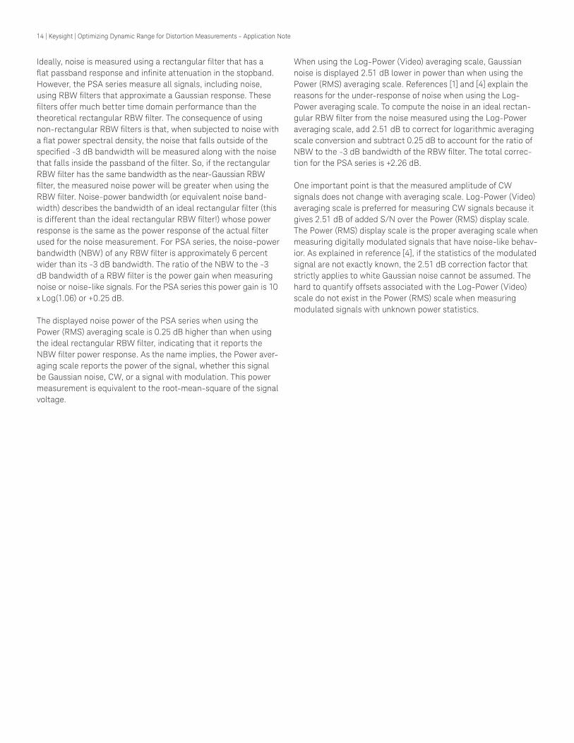
When using the Log-Power (Video) averaging scale, Gaussian

noise is displayed 2.51 dB lower in power than when using the

Power (RMS) averaging scale. References [1] and [4] explain the

reasons for the under-response of noise when using the Log-

Power averaging scale. To compute the noise in an ideal rectan-

gular RBW ilter from the noise measured using the Log-Power averaging scale, add 2.51 dB to correct for logarithmic averaging

scale conversion and subtract 0.25 dB to account for the ratio of

NBW to the -3 dB bandwidth of the RBW ilter. The total correc-

tion for the PSA series is +2.26 dB.

One important point is that the measured amplitude of CW

signals does not change with averaging scale. Log-Power (Video)

averaging scale is preferred for measuring CW signals because it

gives 2.51 dB of added S/N over the Power (RMS) display scale.

The Power (RMS) display scale is the proper averaging scale when

measuring digitally modulated signals that have noise-like behav-

ior. As explained in reference [4], if the statistics of the modulated

signal are not exactly known, the 2.51 dB correction factor that

strictly applies to white Gaussian noise cannot be assumed. The

hard to quantify offsets associated with the Log-Power (Video) scale do not exist in the Power (RMS) scale when measuring

modulated signals with unknown power statistics.

Ideally, noise is measured using a rectangular ilter that has a lat passband response and ininite attenuation in the stopband. However, the PSA series measure all signals, including noise,

using RBW ilters that approximate a Gaussian response. These ilters offer much better time domain performance than the theoretical rectangular RBW ilter. The consequence of using non-rectangular RBW ilters is that, when subjected to noise with a lat power spectral density, the noise that falls outside of the speciied -3 dB bandwidth will be measured along with the noise that falls inside the passband of the ilter. So, if the rectangular RBW ilter has the same bandwidth as the near-Gaussian RBW ilter, the measured noise power will be greater when using the RBW ilter. Noise-power bandwidth (or equivalent noise band-

width) describes the bandwidth of an ideal rectangular ilter (this is different than the ideal rectangular RBW ilter!) whose power response is the same as the power response of the actual ilter used for the noise measurement. For PSA series, the noise-power

bandwidth (NBW) of any RBW ilter is approximately 6 percent wider than its -3 dB bandwidth. The ratio of the NBW to the -3

dB bandwidth of a RBW ilter is the power gain when measuring noise or noise-like signals. For the PSA series this power gain is 10

x Log(1.06) or +0.25 dB.

The displayed noise power of the PSA series when using the

Power (RMS) averaging scale is 0.25 dB higher than when using

the ideal rectangular RBW ilter, indicating that it reports the NBW ilter power response. As the name implies, the Power aver-aging scale reports the power of the signal, whether this signal

be Gaussian noise, CW, or a signal with modulation. This power

measurement is equivalent to the root-mean-square of the signal voltage.


Signal-to-Noise with Excess Noise

The S/N vs. mixer level graph also works when the noise at the

input is greater than the noise loor of the spectrum analyzer, something not all that uncommon, especially when preampliiers are used as part of the measurement system. This excess noise

can stem from devices with relatively low signal-to-noise ratios as

compared with the spectrum analyzer. Some examples of these

devices are signal sources and elements in receiver architectures.

In this discussion, we are concerned with excess broadband

noise, not close-in phase noise.

Figure 2–5 depicts the situation where the external noise from the

DUT is greater than the noise loor of the spectrum analyzer (SA). At higher signal power levels the external signal-to-noise ratio

stays constant. As the input signal power decreases, the external

noise falls below the noise loor of the spectrum analyzer, in which case the S/N decreases in the familiar 1 dB per 1 dB of signal

power reduction.

Figure 2–6 shows how external noise appears on the S/N versus

mixer level graph. At higher powers, the DANL relative to the

power at the mixer stays constant and at lower mixer levels

the S/N curve shows the familiar slope of -1. The SA Noise and

the external noise add as uncorrelated powers such that at the

intersection of the SA noise and the external noise curves, the

combined noise is 3 dB higher than the two individual contrib-

utors alone. The external noise as displayed on the spectrum

analyzer follows the same dependency on RBW setting as the SA

noise, such that for every decade increase in RBW value, both the

SA Noise and the external noise curves shift up by 10 dB on the

dynamic range chart. Figure 2–6. Signal-to-Noise vs. Mixer Level with External Noise Greater than SA Noise

-120

-110

-100

-90

-80

-70

-80 -70 -60 -50 -40 -30

Mixer Level (dBm)

DA

NL

rela

tive

to

Mix

er

Leve

l (d

Bc)

External Noise Combined Noise

SA Noise

Pin(dBm)

Pout(dBm)

SA Noise Floor

S/Nexternal

Delayed Signal

ExternalNoise

Figure 2–5. SA Pout vs. Pin with External Noise


Pin(dBm)

Pout(dBm)

S/D

1N

Output InterceptPoint (dBm)

Fundamental Tone

DistortionProduct

Figure 2–8. Second and Third Order Distortion Spectrum

Second Order Third Order

P P

f0 2f0 2f1-f2 f1 f2 2f2-f1

Signal-to-Distortion versus Mixer Level

Distortion products can also be viewed on the Power-out vs.

Power-in graph. Figure 2–7 shows that Nth order distortion

product amplitudes increase N dB for every dB of fundamen-

tal tone power increase. The signal-to-distortion ratio (S/D)

decreases N-1 dB for every 1 dB of increase in fundamental tone

power. Above a certain power level, however, the spectrum ana-

lyzer gain compresses, at which point the output power no longer

increases in a linear relationship when plotted on a log power

scale. By extrapolating the below gain compression Pout vs. Pin

curves for both the fundamental tone and the distortion products,

the two lines cross at a ictional output power level above gain compression. The output power where these two lines meet is

termed Third Order Intercept (TOI) for third order intermodula-

tion distortion and Second Harmonic Intercept (SHI) for second

harmonic distortion.

For the spectrum analyzer, TOI and SHI are speciied with respect to the power at the input mixer. Another way of thinking about

these speciications is that TOI and SHI are measured assuming 0 dB Input Attenuation. Referring to Figure 2–8, SHI is calcu-

lated as: SHI = P + Δ; where P is the input power minus the Input

Attenuation value and Δ is the dB difference between the second

order distortion product power level and the fundamental tone

power level (Δ is a positive value). TOI is measured assuming two

equal power tones at the input and is calculated as: TOI = P + Δ/2.

In this case P is the power at the input mixer of each tone; P is

not the combined tone power, which would be 3 dB higher. Again

Δ is the power difference between each fundamental tone and

the intermodulation distortion product and is a positive value. If

the two intermodulation products have unequal amplitudes, the product with the higher amplitude is used, giving a worst-case

TOI result.

Having demonstrated the conversion of S/N from the Power-out

versus Power-in graph to the S/N versus mixer level graph, we

can also plot S/D versus mixer level. Figure 2–9 shows distortion

relative to mixer level (or inverted signal-to-distortion) in dBc

units versus the input power at the mixer for second and third

order distortion.

For second order distortion the slope of the S/D versus mixer

level curve is +1, signifying that for every 1 dB increase in power

at the mixer, the S/D decreases 1 dB. For third order the slope of

this curve is +2; for every 1 dB increase in the two fundamental

tone power levels, the S/D decreases by 2 dB. For the second

harmonic curve the 0 dBc intersection point on the y-axis cor-

responds to the SHI value in dBm on the x-axis. In the example

shown in Figure 2–9, the SHI performance of the spectrum ana-

lyzer is +45 dBm. For the third order curve the 0 dBc intersection

point on the y-axis corresponds to the TOI value in dBm. In this

example, the TOI of the spectrum analyzer is +20 dBm.

Figure 2–9. Signal to Distortion versus Power at the Input Mixer

-120

-100

-80

-60

-40

-20

0

Mixer Level (dBm)

-50 -40 -30 -20 -10 0 10 20 30 40 50

Dis

tort

ion

Rela

tive

to

Mix

er

Leve

l (d

Bc) 1

SHITOI

Third Order

2

Second Order

Figure 2–7. Pout vs. Pin Curves for Distortion


The Dynamic Range Chart

Combining the signal-to-noise and the signal-to-distortion versus

mixer level curves into the same graph yields the dynamic range

chart as shown in Figure 2–10.

The dynamic range chart allows a visual means of determining

the maximum dynamic range and the optimum power at the irst mixer where the maximum dynamic range occurs. Using simple

geometry on the curves that make up the dynamic range chart

yields closed form equations for maximum dynamic range and optimum mixer level. Figure 2–10. Dynamic Range Chart

-140-130-120-110-100

-90-80-70-60-50-40

DA

NL

an

d D

isto

rtio

nR

ela

tive

to

Mix

er

Leve

r (d

Bc)

-100 -90 -80 -70 -60 -50 -40 -30 -20 -10 0Mixer Lever (dBm)

Second OrderDistortion

Third OrderDistortion

DANL10 Hz RBW

DANL1 Hz RBW

Second Harmonic Distortion:

Maximum Dynamic Range = ½ SHI - DANL] dB (2–1)

Optimum Mixer Level = ½ [SHI + DANL ] dBm (2–2)

Third Order Intermodulation Distortion:

Maximum Dynamic Range = 2/3 [TOI - DANL] dB (2–3)

Optimum Mixer Level = 1/3 [2 x TOI + DANL] dBm (2–4)

For example, the values in Figure 2–10 are:

DANL = -145 dBm in 10 Hz RBW

TOI = +20 dBm

SHI = +45 dBm

Second Order Distortion in 10 Hz RBW:

Maximum Dynamic Range = 1/2 [45 - (-145)] = 95 dB

Optimum Mixer Level = 1/2 [45 - 145] = -50 dBm

Third Order Intermodulation Distortion in 10 Hz RBW:

Maximum Dynamic Range = 2/3 [20 - (-145)] = 110 dB

Optimum Mixer Level = 1/3 [2 x 20 - 145 ] = -35 dBm


Phase Noisemasks thedistortionproducts

f1 f2

RBW2

RBW1

PhaseNoise

f0 foffset

Figure 2–11b. Phase Noise as

a function of RBW

Figure 2–12. Phase Noise Represented on the Dynamic Range Chart

-140-130-120-110-100

-90-80-70-60-50-40

-100 -90 -80 -70 -60 -50 -40 -30 -20 -10 0

Mixer Level (dBm)

DA

NL

an

d D

isto

rtio

nR

ela

tive

to

Mix

er

Leve

l (d

Bc)

DANL1 Hz RBW

Third OrderDistortion

Phase Noise(Power Scale)

Phase Noise(Log Power Scale)

Equation 2-5.

Total Power = 10 x Log (10^(P1/10) + 10^(P2/10)) [dBm]

where P1 and P2 are the individual power terms in dBm

Adding Phase Noise to the Dynamic Range Chart

Phase noise, due to either the DUT or the spectrum analyzer, can

hide distortion products, as demonstrated in Figure 2–11a. In

this case, the third order intermodulation products fall under the

phase noise skirt, preventing them from being measured.

Like broadband noise, the displayed phase noise loor also changes level with RBW setting, as shown in Figure 2–11b. The

spectrum analyzer phase noise at a particular frequency offset is speciied in dB relative to carrier in a 1 Hz noise bandwidth. This 1 Hz noise bandwidth assumes a phase noise measurement on a

power scale with the over-response due to the ratio of the equiv-

alent noise bandwidth to the -3 dB bandwidth of the RBW ilter removed. The relationship of displayed broadband noise versus

averaging scale depicted in Figure 2–4 also applies to phase

noise. Therefore, if phase noise measurements are to be made

using the Log-Power (Video) scale, which is the preferred display

mode for CW signals, the phase noise value needs to be offset by

-2.26 dBc from its speciied level. When using the Power (RMS) averaging scale, the phase noise is offset by +0.25 dBc from its

speciied value.

Figure 2–12 demonstrates how phase noise appears on the

dynamic range chart. Note that phase at one offset frequency is presented. For this case the speciied phase noise at the particu-

lar offset frequency of interest is -110 dBc/Hz. Using the Log-Power (Video) averaging scale, the phase noise appears to be

-110 minus 2.26 dB or -112.26 dBc normalized to the 1 Hz RBW.

When using the Power display scale, the phase noise appears

to be 2.51 dB higher than with the Log-Power display scale, or

-109.75 dBc normalized to the 1 Hz RBW.

Referring to Figure 2–6 where external noise is shown adding

to the broadband noise of the spectrum analyzer, when two

uncorrelated noise signals combine, the resulting total power is

computed as shown in equation 2–5.

The phase noise and the broadband noise, being uncorrelated,

also follow equation 2–5 when they combine. So, at the intersec-

tion of the phase noise and the DANL curves, assuming both are

shown on the same display scale setting, the resulting total noise

power is 3 dB higher than the two individual contributors.

Figure 2–11a. Phase Noise

Limitations on Dynamic

Range


Noise Adding to the Distortion Product

This section concerns the measurement of CW-type distortion

products measured near the noise loor when using the Log-Power averaging scale. An overview is given here, and references

[4] and [6] explain this subject in greater detail.

When a CW tone amplitude is close to the noise loor, the signal and noise add together as shown in Figure 2–13.

The apparent signal is the signal and noise added together that

the user would see displayed on the spectrum analyzer. Reference

[4] gives this the name S+N for signal-plus-noise. The displayed

signal-to-noise ratio is the apparent signal peak to the broadband

noise (noise level with the CW tone removed). The term, actual

signal-to-noise ratio, means the ratio of the true CW tone peak

amplitude to the broadband noise level. The actual signal-to-

noise ratio is somewhat lower than the displayed signal-to-noise

ratio. Figure 2–14 shows graphically the signal-to-noise ratio error

versus the displayed signal-to-noise ratio. The difference between

the displayed S/N and the actual S/N is the signal-to-noise ratio

error. This graph pertains to CW distortion measurements using

the Log-Power (Video) averaging scale, not the Power (RMS)

averaging scale

To use the graph shown in Figure 2–14, locate the displayed

signal-to-noise ratio on the x-axis, then read off the error on

the y-axis. Subtract this error value from the displayed signal

amplitude to compute the true CW signal amplitude. For example,

suppose the displayed S/N is 3 dB for a displayed signal measur-

ing -100 dBm. The corresponding error is 1.1 dB, which means

that the true signal amplitude is -100 dBm minus the 1.1 dB error

term, or -101.1 dBm. One key observation is that when the CW

tone amplitude is equal to the broadband noise level, that is, 0 dB actual S/N, the displayed S/N is approximately 2.1 dB. For an

error in the displayed S/N to be less than 1 dB, the displayed S/N

should be at least 3.3 dB.

When making distortion measurements on CW-type signals, the

information in Figure 2–14 can be transferred to the dynamic

range chart. Figures 2–15 and 2–16 show how the second and

third order dynamic range curves change as a result of noise

adding to the distortion products.

Below the solid, heavy lines representing distortion-plus-noise,

the CW distortion products are not discernable. This translates

to a reduction in the spectrum analyzer’s maximum dynamic

range. Both the second and third order maximum dynamic ranges

reduce by approximately 2.1 dB when the effect of noise is added

to the CW distortion products displayed on the Log-Power scale.

The corresponding optimum mixer level is offset by +0.5 dB for

second harmonic distortion and by -0.36 dB for third order inter-

modulation distortion. All of these values are relative to the ideal

maximum dynamic ranges and optimum mixer levels given by

equations 2–1 through 2–4.

Figure 2–13. CW Tone Plus Noise

Actual S/N

DisplayedS/N

CW Signal

Apparent Signal

Figure 2–14. S/N error versus displayed Actual S/N for CW Signals using a

Log-Power Display

0.001.002.003.004.005.006.007.008.009.00

10.00

Displayed S/N (dB)0 1 2 3 4 5 6

S/N

Err

or

(dB

)

Figure 2–15. Dynamic Range Chart with Noise Added to the CW Second

Order Distortion Products

Figure 2–16. Dynamic Range Chart with Noise Added to the CW Third Order

Distortion Products

-104

-102

-100

-98

-96

-94

-92

-90

Mixer Level (dBm)

DA

NL

an

d D

isto

rtio

n R

ela

tive

to M

ixer

Leve

l (d

Bc)

-60 -59 -58 -57 -56 -55 -54 -53 -52 -51 -50

Distortion +Noise

SecondOrderDistortion

DANL

-120

-118

-116

-114

-112

-110

-108

-106

-45 -44 -43 -42 -41 -40 -39 -38 -37 -36 -35

Mixer Level (dBm)

DA

NL

an

d D

isto

rtio

n R

ela

tive

to M

ixer

Leve

l (d

Bc)

Distortion +Noise

ThirdOrderDistortion

DANL

Figures 2–15 and 2–16 show the reduced dynamic range assum-

ing no steps are taken to remove the near-noise measurement

errors. The S/N Error versus Displayed S/N graph (Figure 2–14)

indicates that white Gaussian noise adding to a CW signals

results in a predictable amount of error, which is different than an

uncertainty. To regain the lost 2.1 dB of dynamic range, one could

measure the displayed S/N of the near-noise distortion product

and, using the information in Figure 2–14, remove the corre-

sponding error value.


SA Distortion Adding to DUT Distortion

When the amplitudes of the distortion products of the DUT fall

close to the amplitudes of the internally generated distortion

products of the spectrum analyzer, an uncertainty in the dis-

played distortion amplitude results. The DUT distortion products

fall at the same frequencies as the SA generated distortion prod-

ucts such that they add as voltages with unknown phases. The

error uncertainty due to the addition of two coherent CW tones is

bounded by the values shown in equation 2–6.

Equation 2–6 is shown graphically in Figure 2–17. The amplitude error could vary anywhere between the two curves.

For the situation when the internally generated distortion product

is equal in amplitude to the external distortion product, and they are in-phase, the resulting displayed amplitude could be 6 dB

higher than the amplitudes of the individual contributors. For indi-

vidual contributors of equal amplitude that are 180 degrees out of phase, these signals would completely cancel, resulting in no

displayed distortion product.

Equation 2–6 and Figure 2–17 apply without qualiication to harmonic distortion measurements. For two-tone intermodulation

distortion measurements there is an exception. For most distor-

tion measurements, the input power at the spectrum analyzer’s

irst mixer is far below its gain compression level, making the spectrum analyzer a weakly-nonlinear device. Reference [5]

makes the case that for cascaded stages that exhibit a weak non-

linearity, the intermodulation distortion components add in-phase

only. Tests performed on the PSA series conirm this conclusion if the tone spacing is no greater than 1 MHz. Thus for two tone

intermodulation measurements with tone spacing ≤1MHz, the displayed amplitude error due to two distortion products adding

is given by equation 2–7.

To ensure that measurement error due to the combination of DUT

and SA distortion products falls below a given threshold, the

optimum mixer requires readjustment. Unfortunately, this read-

justment has an adverse effect on the maximum dynamic range

available from the spectrum analyzer. The following procedure

helps compute the readjusted dynamic range and the resulting

optimum mixer level needed to ensure that the distortion mea-

surement uncertainty falls below a desired error level.

Start with a desired amount of maximum measurement error and,

using the chart in Figure 2–17, read off the relative amplitudes

corresponding to the desired threshold. For harmonic measure-

ments or two- tone intermodulation measurements whose tone

separations are >1 MHz, use the lower curve as it gives the most

Equation 2-6.

Uncertainty = 20 x Log (1 ±10d/20) dB

where ‘d’ is the relative amplitudes of the two tones in dB

(a negative number).

+ is the case where the DUT and SA distortion products

add in-phase.

- is the case where the DUT and SA distortion products add

180 degrees out of phase.

Equation 2-7.

Amplitude error = 20 x Log (1 + 10d/20) dB

where ‘d’ is the relative amplitudes in dB between the internally

generated distortion and the external DUT generated distortion

amplitudes (a negative number).

conservative result. For IMD measurements with tone separations

≤1 MHz, use the upper curve in Figure 2–16. Or instead, equa-

tions 2–6 and 2–7 could be solved for ‘d’, which is the relative

amplitude value between external and internal distortion product

amplitudes. The relative amplitude value is then used to deter-

mine how to offset the distortion curves in the dynamic range

chart. Either offset the distortion curves up by -d dB or offset the

intercept point by d/(Intercept order -1). For example, for second

order distortion, the effective SHI is offset by ‘d’ and for third

order intermodulation the effective TOI is offset by 1/2 d. By

offsetting the intercept points, instead of offsetting the curves on

the dynamic range chart, equations 2–1 through 2–4 can be used to calculate the optimum mixer levels and the maximum dynamic

ranges.

Figure 2–17. Amplitude Uncertainty due to Two Coherent CW Tone Adding Together

-10.00

-8.00

-6.00

-4.00

-2.00

0.00

2.00

4.00

6.00

8.00

10.00

-25 -20 -15 -10 -5 0

Relative Amplitudes (dB)

Am

plit

ud

e U

nd

ert

ain

ty (

dB

)


Here is an example of how to use the information presented

on near noise and near distortion measurements. Consider the

situation where RBW = 10 Hz, DANL = -155 dBm/Hz and SA TOI

= +20 dBm. The objective is to compute the modiied maximum third order intermodulation dynamic range and the optimum

mixer level. Using equations 2–3 and 2–4, we earlier computed the ideal case maximum dynamic range as being 110 dB and the

corresponding optimum mixer level as being -35 dBm. Suppose

the error uncertainty due to DUT and SA distortion addition is to

be less than 1 dB. Solve equation 2–7 for d:

d = 20 x Log(10 dB Error/20 - 1 ) dB

d = 20 x Log(10 1/20 - 1) dB

d = -18.3 dB

The SA’s effective TOI is computed as SA TOI - d/2 or

+20 - 18.3/2 = +10.85 dBm. Figure 2–18 shows that the distortion

curve has been shifted up by 18.3 dB, corresponding to an effec-

tive loss of 9.2 dB in SA TOI. An intermediate maximum dynamic

range and optimum mixer level can be computed using the new

effective TOI value:

Third Order Distortion in 10 Hz RBW:

Maximum Dynamic Range = 2/3 [10.85 - (-145)] = 103.9 dB

Optimum Mixer Level = 1/3 [2 x 10.85 - 145 ] = -41.1 dBm

Thus in order to drive down measurement error, the loss in

dynamic range is 6.1 dB and the optimum mixer level is shifted

down in power by 6.1 dB.

But we are not done yet. Noise adds to the distortion product,

contributing to a dynamic range loss of 2.1 dB and an optimum

mixer level offset of -0.36 dB. If no steps are taken to remove

this noise error, a inal value for maximum dynamic range equals 101.8 dB with a corresponding optimum mixer level of -41.5 dBm.

The valid measurement region is the area of the dynamic range

chart where distortion interference error is below the desired

error value and the distortion product is discernable above the

noise loor. The valid measurement region for this example is shown in Figure 2–17. Keep in mind that the error due to near

noise addition is still present. This error can be removed with the

aid of the graph in Figure 2–14, resulting in an improvement of

2.1 dB in dynamic range.

One inal note, we mentioned that when measuring TOI with tone spacing ≤1MHz, the DUT distortion products add in-phase with the distortion products generated by the PSA series analyzers,

resulting in what looks like an error term. This situation seems

very similar to the near-noise case, in which the error term can

be subtracted from the displayed amplitude of the CW signal.

Theoretically, the TOI product addition is an error term, and theo-

retically, this error could be subtracted out to regain lost dynamic

range. The dificulty with TOI is with the inability to accurately measure the TOI of the spectrum analyzer. Spectrum analyzer TOI

luctuates with tune frequency due to constantly changing match, as seen by the irst mixer. To accurately measure SA TOI in the hopes of removing the error term, the same input match would

be required for both the SA TOI measurement as well as the inal DUT measurement. Removing the TOI related error term is not

impossible, but for practical reasons it is best to consider the

error term as an uncertainty that cannot be accurately removed

from the measurement.

Figure 2–18. Dynamic Range Chart Showing Valid Measurement Region for <1

dB Measurement Uncertainty for Third Order IMD

-120-115-110-105-100-95-90-85-80-75-70

-55 -50 -45 -40 -35 -30 -25

Mixer Level (dBm)

DA

NL

an

d D

isto

rtio

n R

ela

tive

to M

ixer

Leve

l (d

Bc)

Valid MeasurementRange

9.2 dB

18.3 dB


measurements on the Log-Power (Video) scale and the Power

(RMS) scale. However, if the PDF of the digitally modulated signal

is not known exactly, which is usually the case, then the 2.51 dB

offset does not necessarily hold true. The Power (RMS) averaging

scale must be used for digitally modulated signals as this scale

avoids the uncertainties incurred when computing the

amplitudes on the Log-Power (Video) averaging scale.

The Peak detector and the Normal detector should not be used

for measurements on digitally modulated signals. These detec-

tors report the peak amplitude excursions that occur between

display measurement cells, thus overemphasizing the amplitude

peaks of noise and noise-like signals. The Sample detector, by

contrast, reports the signal amplitude that occurs at the display

measurement cell (sometimes referred to as display “bucket”),

which does not peak bias the measurement. The PSA series

analyzer has another detector, called the Average detector, which

reports the average of the data across each display bucket.

When using the Average detector, the longer the sweep time,

the greater the amount of averaging. Either the Sample detector

or the Average detector should be used for measurements on

digitally modulated signals.

The Video Bandwidth (VBW) ilter reduces the amplitude luctu-

ations of the displayed signals and, depending on the spectrum

analyzer, is placed either before or after the linear to logarithmic

conversion process in the intermediate frequency (IF) chain. One new feature in the PSA series analyzer not found in previous

generation Keysight spectrum analyzers is that the VBW ilter does not affect the power summation performed when using the

Power (RMS) scale. When using spectrum analyzers in which the

VBW ilter is placed after the linear to logarithmic conversion process, the user is cautioned to keep the VBW ≥3 x RBW for the

measurement of signals that are random in nature. This ensures

that averaging occurs on the Power scale and avoids the offsets

that occur on the log scale. When using the Power (RMS) aver-

aging scale, the PSA series analyzer allows an arbitrarily narrow

VBW setting without the worry that the measured amplitude will

contain log scale uncertainties. This allows more lexibility to use the VBW to reduce the measured amplitude variance of the

digitally modulated signal.

Part III: Distortion Measurements on Digitally Modulated Signals

In Part II we concentrated on the distortion measurements of CW

signals containing no modulation. In Part III, we turn our atten-

tion to out-of-channel leakage measurements, such as adjacent

channel power (ACP) and alternate channel power on digitally

modulated signals. Optimizing the mixer level of the spectrum

analyzer is equally as important for these types of distortion mea-

surements as it is for distortion measurements on CW signals.

However, setting the mixer level for digitally modulated signals

requires different considerations than what we will discuss here in Part III.

Reference [4] states that under conditions where the measure-

ment bandwidth is much narrower than the modulation band-

width (BWm) of a digitally modulated signal, the signal exhibits

noise-like statistics in its amplitude distribution. In most practical

cases, the spectrum analyzer RBW is much narrower than BWm

and satisies the above condition. For example, when measur-ing adjacent channel power ratio (ACPR) on an IS-95 CDMA

signal with a 1.23 MHz BWm, the speciied measurement RBW is 30 kHz. Why is the fact that the signal exhibits noise-like behav-

ior important? First, unlike with CW tones, greater care must be

exercised in selecting the display mode, both the display detector

and the averaging scale, when measuring digitally modulated

signals. Second, both the displayed main channel power and the

displayed spectral regrowth (that is, distortion products) are a

function of the RBW setting of the spectrum analyzer. Finally, the

manner in which the digitally modulated signal’s noise-like dis-

tortion components and broadband noise add together behaves

differently than when the distortion is CW. These points will all be

discussed in greater detail in the following.

Choice of Averaging Scale and Display Detector

One of the irst considerations when measuring digitally modu-

lated signals is the choice of the averaging scale (Log-Power vs.

Power scale). In order for the digitally modulated signal to behave

exactly like noise, its amplitude versus time characteristic must

possess a Gaussian Probability Density Function (PDF). If the

Gaussian PDF is assumed then the displayed main channel power

spectral density (PSD) follows the same rules as white noise,

where a 2.51 dB displayed amplitude difference occurs between


Maximizing Spectrum Analyzer Dynamic Range

Three mechanisms inherent to the spectrum analyzer limit its

dynamic range when measuring out of channel distortion on

digitally modulated signals. These mechanisms are: the spectrum

analyzer noise loor, the spectrum analyzer phase noise and the spectrum analyzer intermodulation distortion. The noise loor is always a limit as it is with CW distortion measurements. Phase

noise and intermodulation, however, are limits that depend on

such parameters as channel separation and modulation band-

width. In other words, in the majority of cases, depending on the

modulation format, phase noise or intermodulation will limit the

dynamic range of the spectrum analyzer.

Signal-to-Noise of Digitally Modulated Signals

The spectrum analyzer displays the main channel PSD at a level

lower by 10 x Log(BWm) than the amplitude of a CW tone with

equal power. Therefore, the displayed S/N of the digitally mod-

ulated signal is reduced by 10 x Log(BWm). Figure 3–1a shows

this effect. Furthermore, the displayed amplitude and displayed

broadband noise are functions of the RBW setting which, unlike

the CW case, renders the S/N independent of the RBW. See

Figure 3–1b.

The displayed main channel PSD is Pch - 10 x Log(BWm/RBW) +

10 x Log(NBW/RBW). Pch is the total signal power and NBW is

the noise power bandwidth of the RBW ilter used for the mea-

surement. For the PSA series analyzer NBW/RBW is 1.06 or 10

x (NBW/RBW) = 0.25 dB. The following is an example for com-

puting the displayed amplitude of a -10 dBm IS-95 CDMA signal

measured with a 30 kHz RBW ilter setting:

Average Displayed Amplitude =

Pch – 10 x Log(BWm/RBW) +10 x Log(NBW/RBW)

Average Displayed Amplitude =

-10 - 10 x Log(1.2288 MHz/30 kHz) + 10 x Log(1.06)

Average Displayed Amplitude = -25.9 dBm

Broadband noise on the Power (RMS) averaging scale appears at

the speciied DANL + 10 x Log(RBW) + 2.51 + the Input Attenuator

setting. So for a spectrum analyzer with a DANL of -155 dBm/

Hz measured with a 30 kHz RBW ilter with 10 dB of Input Attenuation, the displayed noise level on the Power Scale is: -155

+ 10 x Log(30 kHz) + 2.51 + 10 = -97.7 dBm. The signal-to-noise

ratio computes to 71.8 dB.

For purposes of plotting the S/N on the dynamic range chart, it

is best to think of the channel power in terms of the power at the

input mixer of the spectrum analyzer; call this power MLch. MLch

= Pch - Input Attenuation. Thus, S/N as a function of power at the

irst mixer is given by equation 2–8.

Figure 3–1a. Displayed Amplitude of a CW Tone and a

Digitally Modulated Signal with Equal Powers

Figure 3–1b. Displayed Amplitude of Both Digitally

Modulated Signal and DANL varies with RBW

PSD in 1 Hz BW

CW Tone

10*Log(BWm)

RBW1

RBW2

S/N1S/N2

Figure 3–2. S/N vs. Mixer Level for Digitally Modulated Signals

-120-110-100-90-80-70-60-50-40-30-20-10

0

-100 -90 -80 -70 -60 -50 -40 -30 -20 -10

Mixer Level (dBm)

DA

NL

Rel

ativ

e to

Mix

er

Leve

l (dB

c) a

nd -

S/N

(dB

)

-S/N of aModulatedSignal

DANL in1 Hz RBW

10Log[BWm] + 2.26 dB

Equation 2–8 makes it evident that for digitally modulated signals, the S/N is a function of the modulation bandwidth. Wider

bandwidths lead to a lower S/N. Figure 3–2 shows the dynamic

range chart with the S/N plotted against the input power at the

irst mixer for an IS-95 CDMA modulated signal. The S/N curve of the modulated signal is offset from the DANL curve by 10 x

Log(BWm) - 2.26.

Equation 2-8.

S/N as a Function of Power at the irst mixerS/N = MLch -10 x Log(BWm) +10 x Log(NBW/RBW) - DANL -2.51 [dB]

S/N = MLch - DANL -10 x Log(BWm) - 2.26 [dB]


Spectral Regrowth Due to Spectrum Analyzer Intermodulation Distortion

Third, and in some cases ifth order intermodulation distortion of the spectrum analyzer create distortion products that fall outside

of the main channel. Unlike power ampliiers, and especially power ampliiers with feed-forward architectures, the spectral regrowth internal to the spectrum analyzer can easily be approx-

imated with simple algebra. The analysis of spectral regrowth

generated by spectrum analyzer intermodulation distortion relies

on the premise that when the power at the input mixer is far

below gain compression power level (by at least 15 dB), the

spectrum analyzer behaves as a weakly-nonlinear device. Such

a device has a voltage-in to voltage-out transfer function given

by the power series: Vo = a1Vi + a2Vi2 + a3Vi

3 + . . . + anVin. For

spectrum analyzer front ends, the power series does an excellent

job of predicting the frequencies of the intermodulation dis-

tortion terms and their relative amplitudes. As the input power

approaches the spectrum analyzer gain compression level, the

power series approximation no longer hold true, indicating the

limitation of this equation to relatively low power levels.

Spectral regrowth modeling for the spectrum analyzer front

end begins by breaking up the main channel into a series of

equal spaced divisions in the frequency domain. Each division is represented by a CW tone whose power is the same as the

total power in that particular division. Figure 3–3a depicts this

interpretation of the spectral regrowth model. Each CW tone

representing a segment of the main channel interacts with all of

the other CW tones creating intermodulation distortion products.

Intermodulation products resulting from different tones start

combining with each other, with the most products adding at the

edges of the main channel. It has been determined empirically

that the individual distortion products add as voltages using the

20 Log( ) relationship. In most cases a log amplitude scale is used

that displays the spectral regrowth falling off on a curve as shown

in Figure 3–3b. For third order distortion, the upper and lower

spectral regrowth bandwidths are only as wide as the modulation

bandwidth of the digitally modulated signal. The third order dis-

tortion extends out in frequency away from the main channel by one modulation bandwidth and ifth order extends by two mod-

ulation bandwidths. Third order distortion dominates in adjacent

channel measurements. For alternate channel measurements,

ifth order distortion becomes a concern.

Spectral regrowth due to intermodulation distortion is noise-like,

implying that the main signal power to spectral regrowth power

ratio is independent of the spectrum analyzer RBW setting. In

other words, the displayed main channel PSD and the spectral

regrowth PSD both vary by the 10 x Log(RBW) relation. Another

implication is that when the distortion approaches the system

noise loor, the distortion and noise add as uncorrelated powers using the relationship:

Figure 3–3b. Spectral Regrowth as Displayed on the Log Scale

3rd OrderDistortion

5th OrderDistortion

BWm BWm BWm BWm BWm

LowerAlternateChannel

LowerAdjacentChannel

MainChannel

UpperAdjacentChannel

UpperAlternateChannel

Figure 3–3a. Spectral Regrowth Generated Within the Spectrum Analyzer

can be Modeled by Treating the Digital Signal as a Series of CW Tones

Equation 3-1

Total Power = 10 x Log(10 Noise Power / 10 +10 Distortion Power / 10 ) dBm

where Noise Power is the system noise in dBm and Distortion

Power is the intermod-generated spectral regrowth in dBm.

20

15

10

5

0

-5

0.5 0.75 1 1.25

Foffset / BWm

TOI O

ffse

t (d

B)

Pk/Avg (dB)

5.5

11

16

Figure 3–4. Effective TOI of Digitally Modulated Signal versus Frequency Offset from Main Channel

Calculating the level of third order generated spectral regrowth

depends on the frequency offset from the main channel center frequency and the peak-to-average-ratio of the signal. A further complication is whether or not the adjacent channel

measurement is made at ixed offset frequencies, as with IS-95 CDMA, or the measurement, is an integrated power measurement

as with W-CDMA. For measurements at ixed offset frequencies, Figure 3–4 can be used to estimate the third order spectral

regrowth for the PSA series analyzer. Note that these results

cannot be generalized for other spectrum analyzers. Shown is the

TOI offset from the two-tone TOI performance of the spectrum

analyzer versus the frequency offset from the center of the main channel for three different peak-to-average ratios.


The best way to show how to use Figure 3–4 is through illustra-

tion. Suppose the ACPR is to be calculated at an offset of 885 kHz

for an IS-95 CDMA signal whose modulation bandwidth is 1.23

MHz and peak-to-average ratio is 11 dB. The Foffset/BWm ratio =

.885/1.23 = 0.72. From Figure 3–4, the TOI offset at Foffset/BWm

of 0.72 is +3 dB. Suppose the spectrum analyzer has a two tone

TOI of +20 dBm, the effective TOI at 885 kHz offset would be 20

dBm + 3 dB or +23 dBm. If the power at the spectrum analyzer’s

input mixer is -10 dBm, the spectral regrowth can be calculated

by manipulating the equation: TOI = P + Δ/2. In this case, Δ is the

dB difference of the main channel PSD to the third order spectral

regrowth. For the example in this discussion, this power differ-

ence is computed as

Δ = 2*(TOI - P)

Δ = 2 x (23 - (-10))

Δ = 66 dB

So at an offset of 885 kHz from the main channel center fre-

quency, the third order spectral regrowth generated within the spectrum analyzer would be 66 dB below the main channel

average PSD.

For measurements that rely on an integrated power measure-

ment across the adjacent channel, predicting the level of spectral

regrowth due to third order distortion depends on modulation

bandwidth and channel spacing. Channel spacing is important

because it determines the unused frequency band between channels, where the spectral regrowth can be ignored. W-CDMA

is one important class of digitally modulated signals that use an

integrated measurement. For W-CDMA with 3.84 MHz symbol

rate and a 5 MHz channel spacing, the effective TOI offset is

given in Table 3–1.

This table shows how to calculate the integrated adjacent channel

power due to third order distortion. For example, suppose the

W-CDMA signal has a peak-to-average ratio of 11 dB and the

spectrum analyzer has a two-tone TOI of +20 dBm. The effec-

tive TOI with a W-CDMA modulated signal is 20 dBm + 4 dB or

+24 dBm. Manipulating the math as in the previous example, the

spectral regrowth in the adjacent channel, assuming -10 dBm

power at the input mixer, is:

Δ = 2 x (24 - (-10))

Δ = 68 dB

That is, the power integrated across the adjacent channel is 68 dB

below the power integrated across the main channel.

Phase Noise Contribution

Just as internally generated phase noise can limit the dynamic

range when measuring CW tones, phase noise also places a lim-

itation on the dynamic range when measuring digitally modulated

signals. The model used to calculate intermodulation distortion

of a digitally modulated signal also proves useful in showing how

the phase noise adds to the spectral regrowth in the adjacent

channel. In Figure 3–5, the main channel is divided into segments

of equal frequency width with a CW tone representing the power in each segment.

Associated with each CW tone is a phase noise skirt. The

phase noise power contributed by individual tones at any given

frequency add in an uncorrelated fashion (that is, the 10 Log( ) relationship). The closer the frequency offset is to the main channel, the greater the summation of the phase noise power.

The end result is a reduction in the phase noise dynamic range of

roughly 10 x Log(BWm). For example, suppose at 100 kHz offset,

the spectrum analyzer’s speciied phase noise is -118 dBc/Hz. With a modulation bandwidth of 1.23 MHz, the phase noise power

at 100 kHz away from the edge of the main channel relative to

the PSD of the main channel would be -118 + 10 x Log(1.23 x 106)

+0.25 = -56.85 dB (the 0.25 dB term is the 10 x Log(NBW/RBW)

discussed earlier). This relative phase noise power is not exact,

because at any given frequency outside of the main channel, the phase noise derives from contributors that span the width of the

main channel. Therefore, use the 10 x Log(BWm) as a irst order guide and that is probably within a couple dB of the true phase

noise. From the depiction in Figure 3–5, for narrowly spaced

channels, the phase noise can be a serious limitation for ACPR

measurements.

Table 3–1. Effective TOI Offset for W-CDMA

Pk/Avg (dB) TOI Offset (dB)

5.5 7.5

11 4

14.5 2

Figure 3–5. Phase Noise Contribution of a Digitally Modulated Signal

Individual Phase Noises add as uncorrelatedpowers


Dynamic Range Chart for Digitally Modulated Signals

We now have all the ingredients to create the dynamic range

chart when making distortion measurements on digitally

modulated signals. Remember, the goal is to determine the

optimum input power at the mixer, which is a natural outcome

of the dynamic range chart. Unfortunately, the dynamic range

chart for digitally modulated signals is highly format depen-

dent. Parameters such as modulation bandwidth and channel

spacing— whether or not the ACPR measurement is at ixed offset frequencies or is an integrated power measurement—and the peak-to-average ratio of the main channel signal all affect

the formation of the dynamic range chart. While it is impossible

to generalize the dynamic range chart, we can get a feel for the

considerations involved in constructing a suitable dynamic range

chart by showing a couple of speciic examples.

Figure 3–6 shows the dynamic range chart for IS-95 CDMA with

an 11 dB peak-to-average ratio measured at a single offset fre-

quency of 885 kHz. The parameters used to construct this chart are: modulation bandwidth = 1.23 MHz, DANL = -155 dBm/Hz,

TOI = 20 dBm + 3 dB offset to account for the 11 dB peak-to-

average ratio, Fifth Order Intercept = +12 dBm, and phase noise =

-132 dBc/Hz at an offset of 270 kHz. The frequency offset value used to approximate the phase noise results from the following

computation: the half-bandwidth of the measurement channel is

(1.23 MHz / 2), or 615 kHz. At a measurement frequency 885 kHz away from the center of the main channel, the frequency differ-ence between the measurement frequency and the edge of the main channel is 885 kHz minus 615 kHz, or 270 kHz.

A few observations can be made regarding Figure 3–6. First,

because the measurement frequency is only 270 kHz away from the edge of the main channel, phase noise is the limiting mecha-

nism for dynamic range. Fifth order intermodulation distortion is

negligible. Third order intermodulation distortion and broadband

noise are minor contributors in the region of maximum dynamic

range. The optimum mixer level is nearly 20 dB higher than the

mixer level for the two-tone intermodulation distortion shown in

Figure 2–10.

Figure 3–7 shows the dynamic range chart for W-CDMA. Again,

the peak-to-average ratio for the signal is 11 dB. The mea-

surement uses integrated power across both the main and the

adjacent channel as opposed to the single frequency measure-

ment for IS-95 CDMA. The parameters used to construct this

chart are: symbol rate = 3.84 MHz, channel spacing = 5 MHz,

DANL = -155 dBm/Hz, TOI = 21 dBm + 4 dB offset to account for

the 11 dB peak-to-average ratio, Fifth Order Intercept = +12 dBm,

and phase noise = -150 dBc/Hz at an offset of 1.17 MHz. The

frequency offset used to estimate the phase noise contribution results from the fact that the frequency difference between the edge of the main channel and the edge of the adjacent channel is

1.17 MHz.

Figure 3–6. Dynamic Range Chart for IS-95 CDMA at 885 kHz Offset

-40 -35 -30 -25 -20 -15 -10 -5 0

-50

-55

-60

-65

-70

-75

-80

-85

Mixer Level (dBm)

Sp

ect

ral R

eg

row

th R

ela

tive

to M

ain

Ch

an

nel P

ow

er

(dB

)

Noise

PhaseNoise 3rd

Order

5th Order

Figure 3–7. Dynamic Range Chart for W-CDMA

-40 -35 -30 -25 -20 -15 -10 -5 0

-55

-60

-65

-70

-75

-80

-85

-90

Mixer Level (dBm)

Sp

ect

ral R

eg

row

th R

ela

tive

to M

ain

Ch

an

nel P

ow

er

(dB

)

Noise

PhaseNoise

3rd Order

5th Order

Because of the 1.17 MHz spacing between channel edges, the

phase noise is considerably lower than with the IS-95 CDMA

example. In fact, phase noise is not a signiicant contributor at all. In the region of maximum dynamic range, ifth order intermodu-

lation distortion is also not a signiicant contributor. Third order intermodulation distortion spectral regrowth and broadband

noise are the only limitations in the region of highest dynamic

range. Notice that the range of mixer levels where the dynamic

range is maximized is narrower than for the IS-95 CDMA case.

Optimum mixer level is about -13 dBm.

Figure 3–7 can also be used to interpret the optimum mixer level

for the alternate channel power measurement. In the alternate

channel, as depicted in Figure 3–3b, the third order distortion

products do not exist, leaving only the ifth order distortion contributing to intermodulation generated spectral regrowth. For

the PSA series, phase noise power stays at a near constant value

between 1 and 6 MHz offsets. Thus the phase noise curve in

Figure 3–7 used for the adjacent channel applies with little error

for the alternate channel measurement. For this measurement the

optimum mixer level is about -5 dBm.


Measurement Error Due to SA Spectral Regrowth Adding to DUT Spectral Regrowth

For CW distortion, we demonstrated that to reduce the measure-

ment error, the DUT and spectrum analyzer distortion product

levels must be offset by an amount dictated by the desired

measurement error. For digitally modulated signals, a similar

consideration must be taken into account. In the case of digitally

modulated signals, the level of intermodulation generated spec-

tral regrowth of the spectrum analyzer must be below the DUT

spectral regrowth by a calculated amount.

When the amplitude of the DUT’s spectral regrowth falls near

the spectral regrowth generated within the spectrum analyzer,

the two add in a manner dependent on the characteristics of the

modulation format. For extremely low peak-to-average ratios, the

distortion products add, approximately, as uncorrelated powers.

As the peak-to-average ratio increases, the spectral regrowth

levels of the DUT and the SA add in a fashion consistent with the

power addition of correlated signals. The conservative approach

would be to use equation 2–7 to estimate differences in DUT and SA spectral regrowth levels as a function of the desired amount

of measurement uncertainty. Once the desired spectral regrowth

level difference is calculated, the information can be applied to

the dynamic range charts to estimate the measurement dynamic

range and the corresponding mixer level. Using the example

in Part II where less than 1 dB of distortion related error was

desired, we apply the same +18.3 dB y-axis offsets to the third

and ifth order curves in the dynamic range charts for digitally modulated signals. For the IS-95 example where phase noise

mostly limits the ACPR measurement, the effect of offsetting

the third order curve is not very signiicant to the overall ACPR dynamic range. But for the W-CDMA example, where S/N and

third order distortion limit the ACPR dynamic range, offsetting the

third order curve has the same effect on dynamic range as with

the CW example where dynamic range is reduced by 6.1 dB and

the optimum mixer level is shifted 9.2 dB lower.


In Parts II and III we demonstrated that in order to maximize the

dynamic range of the spectrum analyzer, the power at the input

mixer must be optimized. Now in Part IV we begin discussing

some block diagram characteristics speciic to the PSA series that may prove useful in achieving the optimum mixer level.

Input Attenuator Resolution

Unless the mixer level can be optimally set, the full dynamic

range performance of the spectrum analyzer cannot be achieved.

Controlling the Input Attenuator provides an easy, and a very

accurate, means of controlling the power at the input mixer. If the

step resolution of the Input Attenuator is too coarse, then setting

the optimum mixer level may prove to be very dificult. Figure 4–1 shows the limitation of the achievable dynamic range due to the

resolution of the Input Attenuator.

If the Input Attenuator is adjusted too high in value, broadband

spectrum analyzer noise limits the achievable dynamic range

and if the Input Attenuator is adjusted too low in value, inter-

nally generated distortion limits the dynamic range. Figure 4–1

depicts the worst case situation where dynamic range is equally limited by noise or distortion as the Input Attenuator toggles

between two adjacent settings. One may get lucky and a particu-

lar attenuation setting may allow an optimal setting for the mixer

level, but in general this luck cannot be relied upon. The potential

dynamic range given up is the difference between the maximum

dynamic range and the achievable dynamic range in the worst

case scenario. Clearly, a iner resolution in the input attenuator allows more control of the power at the input mixer, which in turn

minimizes the dynamic range that is given up.

If one takes the simplistic view that maximum dynamic range

occurs at the intersection of the noise and the distortion product

curves, then the dynamic range given up can be substantial

unless a very ine resolution of the Input Attenuator step size is used. However, as indicated earlier, when the distortion amplitude

approaches the noise loor, the noise and distortion add giving a curve that is more of a trough where the maximum dynamic

range occurs. In this case the sensitivity of achievable dynamic

range versus attenuator step size is not nearly as great as in the

simplistic view.

Part IV: PSA Architectural Effects on Distortion Measurements

Figure 4–1. Attenuator Step Size Governs the Ability to Achieve the

Optimum Mixer Level

-117

-115

-113

-111

-109

-107

-105

-50 -48 -46 -44 -42 -40 -38 -36 -34

Mixer Level (dBm)

DA

NL

an

d D

isto

rtio

nR

ela

tive

to

Mix

er

Leve

l (d

Bc)

AttenuatorStep Size

Potential Dynamic Range Given UpWorst Case DR

due to insufficientattenuator step size

Table 4–1 summarizes the dynamic range given up versus attenu-

ator step size for three scenarios: the simplistic view where noise

and distortion curves meet at a point, CW type distortion on the

Log-Power (Video) averaging scale, and noise-like distortion on

the Power (RMS) averaging scale where the noise and distortion

add as uncorrelated powers. With the simplistic view, one is led

to believe that even iner than 1 dB input attenuator resolution is warranted in order to minimize the lost dynamic range. However,

for the more realistic cases where noise adds to the near-noise

distortion products, the dynamic range given up is not nearly as

great.

The PSA series offer an Input Attenuator with a 2 dB step size.

This allows the user to ine tune the mixer level so that in the worst case, only 0.28 dB of potential dynamic range is given up.

One could use external ixed attenuators to achieve the same results as the internal step attenuator. However, convenience

is certainly sacriiced and, more importantly, so is accuracy. External attenuators lack the frequency response calibration that is assured when using the Input Attenuator

of the PSA series analyzers.

Table 4–1. Potential Dynamic Range Given up [dB] versus Attenutor Step Size [dB].

Attenuator Step Size (dB)

Simplistic View

CW distortion adding to noise on the Log-Power scale

Noise-like distortion adding to noise on the Power scale

10 6.7 4.7 4.1

5 3.3 1.6 1.3

2 1.3 .28 .23

1 .67 .08 .06


Internal Filtering

Although knowing the internal architecture of the spectrum ana-

lyzer seems an unnecessary burden, some simple concepts such

as the internal ilters may help in achieving more dynamic range performance when making distortion measurements.

Figure 4–2 shows a highly simpliied block diagram of the PSA series front end.

Two paths exist: lowband for tuned frequencies less than 3 GHz and highband for tuned frequencies from 3 to 26.5 GHz. Lowband path is broadband in that all signals that fall below 3 GHz are

present at the input of the lowband mixer. Highband path, by

contrast, uses a tuning preselector ilter whose 3 dB bandwidth varies from 40 MHz at 3 GHz to more than 80 MHz at 26.5 GHz.

When measuring harmonic distortion, there is a clear demarca-

tion for fundamental frequencies whose harmonics fall above and below 3 GHz. For harmonics that fall below 3 GHz, the lowband

irst mixer contributes its internally generated distortion to the measurement. However, once the distortion frequency falls above 3 GHz, the highband path’s preselector greatly attenuates the

fundamental tone power before it can reach the highband mixer.

The PSA series speciication sheet shows that the SHI perfor-mance makes a dramatic improvement for source frequencies above 1.5 GHz.

One should also be aware of the potential of overloading the front

end when the lowband path is selected. The PSA series specify a

gain compression level that is the total power at the input mixer

at which the gain of the spectrum analyzer drops by 1 dB. That

is, if the power at the input mixer is at the gain compression level,

spectral components of the displayed signal could be as much as

1 dB lower than when the mixer level is less than -10 dBm. This

is important when working in a multi-tone environment and the

frequency span of the spectrum analyzer is suficiently narrow to remove large signals from view. For the highband path, knowl-

edge of the preselector bandwidth can help extend the gain com-

pression performance of the spectrum analyzer. The PSA series

speciication for gain compression in highband is for the power at the mixer. As the analyzer tunes away from a particularly strong

signal, the preselector ilter will attenuate this signal before it reaches the highband mixer. So in a multi-tone environment, if the

spectrum analyzer is tuned several preselector bandwidths away

from a strong signal, we can reduce the input attenuation, thus

improving dynamic range without worrying about front end com-

pression affecting the amplitude accuracy of the measurement.

One last item regarding internal iltering is the iltering in the inal IF of the PSA series. This discussion assumes that the PSA series

analyzer is in swept analysis mode as opposed to FFT analysis

mode. Swept analysis mode is selected by activating the Mode

Setup hardkey, FFT & Sweep softkey, Sweep Type set to Swp.

The maximum mixer level before the inal IF overloads is within 2 dB above -10 dBm. In fact, the user cannot set the reference

level such that the mixer level is above -10 dBm. Signals above

this level are displayed above the top of the screen and a ‘Final IF

Overload’ message appears on the display. However, the speci-

ied gain compression level is more than 10 dB above this level, which can yield 10 dB more compression-to-noise dynamic range

out of the spectrum analyzer over what is at irst apparent. When measuring a small signal in the presence of a large signal, irst measure the amplitude of the large signal with suficient input attenuation to drop the mixer level below -10 dBm. When mea-

suring the small signal, tune the start and stop frequency such that the large signal is at least 15 kHz or 15 x RBW setting (which-

ever is greater) outside of the frequency range of the spectrum analyzer. For example, if a large signal is present at 1 GHz and the

user wants to measure a small signal above 1 GHz and a 1MHz

RBW setting is selected, ensure that the start frequency of the spectrum analyzer is greater than 1.015 GHz (1 GHz + 15 x

1 MHz). Once the frequency span is set such that the large signal is no longer in view, the Input Attenuator can be adjusted lower

to improve the measurement sensitivity. However, care must be

observed when lowering the Input Attenuation so that the power

at the mixer is still below the speciied compression level.

3 GHz

DC to 3 GHz

Input Attenuator

RFInput

HighbandMixer

LowbandMixer

3—26.5 GHzHighbandPreselectionFilter

Figure 4–2. PSA Series Front End


Internal PreampliierThe PSA series offer an internal lowband 100 kHz—3GHz pream-

pliier as an option (Option 1DS). The preampliier is placed in the block diagram after the input attenuator, but before the lowband

input mixer. The preampliier places roughly 28 dB of gain ahead of the lowband irst mixer, which lowers the system DANL by about 15 dB. Normally, the preampliier is used to measure extremely low amplitude spurious signals, signals that would

normally fall close to or below the noise loor in the non-pream-

pliier path. However, it is worth mentioning the behavior of the preampliier path if this path is selected when making distortion measurements.

As previously mentioned, the preampliier lowers the noise loor of the spectrum analyzer by about 15 dB. The preampliier does not signiicantly add distortion to the system, however it does increase the power at the input mixer by the nominal gain value of

28 dB. This has the effect of lowering system SHI, TOI, and gain

compression level by around 28 dB. The result is a drop in the

second order dynamic range of 6.5 dB, a drop in the third order

dynamic range of 8.5 dB, and a drop in the compression to noise

dynamic range of 13 dB.

Figure 4–3 shows the dynamic range chart for the internal pream-

pliier path selected. For both second order dynamic range and third order dynamic range, the optimum mixer levels are consid-

erably lower than with the non-preampliier path. This may be of some beneit for low level applications where there is not enough DUT power to reach the optimum mixer level of the non-

preampliier path.

Figure 4–3. Dynamic Range Chart with the Internal Preamp Selected

-120-115-110-105-100-95-90-85-80-75-70-65-60

-100 -95 -90 -85 -80 -75 -70 -65 -60 -55 -50

Mixer Level (dBm)

DA

NL

an

d D

isto

rtio

n

Rela

tive

to

Mix

er

Leve

l (d

Bc)

1 Hz DANLSecond OrderDistortion

Third Order Distortion


In this inal Part, we cover a few miscellaneous items that could impact the distortion measurement.

Reducing Source Intermodulation Distortion

Equally as important as ensuring proper coniguration of the spectrum analyzer used to measure intermodulation distortion is

that the sources used to generate the multi-tone stimulus be free

of IMD. IMD generated in the sources is normally a result of insuf-

icient isolation between the sources. Figure 5–1 shows a highly simpliied block diagram of a signal source.

The signal source generates the CW tone at frequency f1 . A

second CW source at frequency f2 is connected to this signal

source by some means of power combination. Signal energy

from the second source enters the output port of the source and,

because the output coupler does not have ininite isolation, a portion of the f2 signal leaks into the coupled port of the output

coupler. Both the signals at f1 and f2 are detected, which creates

a beat note at a frequency of |f2 - f1|. If this beat note is lower

in frequency than the loop bandwidth of the automatic leveling control (ALC) circuit, the ALC will respond to this signal causing

AM sidebands on the output signal. Unfortunately, the AM side-

bands fall right at the intermodulation distortion product frequen-

cies, resulting in what appears as IMD out of the source.

The solution to improving source generated IMD is to prevent the

energy of the second source signal from entering the output

port of the signal source. The required isolation between the two sources is dependent on the susceptibility of the signal source

to signals entering the output port as well as the acceptable AM

sideband level needed for the TOI measurement.

Some of the better power combination techniques are:

Wilkinson Power Combiners— these can achieve greater than

30 dB isolation.

Class A Ampliiers at the output of the sources—important to not use ampliiers that have leveling control circuitry of their own.

Fixed Attenuators—these should be used in conjunction with

power splitters and ampliiers.

Isolators—the downside is their relatively narrow bandwidth.

Couplers—high directivity couplers needed.

Some power combiners that do not work very well are two- and

three-resistor splitters. The temptation to use these are great due

to their very wide bandwidth. However the two-resistor splitter

only has 12 dB of isolation and the three-resistor splitter only has

6 dB of isolation. A device that should never be used is the T (BNC

T and smb T are examples). These not only have zero isolation, but

also they present a very poor match to the DUT, which can have

an adverse effect on the measurement accuracy.

Part V: Enhancing Distortion Measurements

LevelAdjust

OutputAmp

PowerDetector

f1

f1

f2

f1f2

ALC

Figure 5–1. Simpliied Output Section of a Signal Generator


Effects of Harmonics on Intermodulation Distortion

When measuring intermodulation distortion, an important con-

sideration is the harmonic content from the sources as well as

the device under test. Two-tone IMD will be used in the following

example, however this analysis can be extrapolated to multi-tone

IMD.

Suppose a nonlinear device, either the DUT or the spectrum ana-

lyzer used to make the IMD measurement, can be modeled using

the power series up through the third order term:

Equation 5-1

Vo = a1Vi + a2Vi2 + a3Vi

3

Now subject this nonlinear device to the following two-tone input

signal:

Equation 5-2

Vi = A x Cos(ω1t) + B x Cos(ω2t) + C x Cos(2ω1t)

For a two-tone IMD measurement, amplitudes A and B are set

to be the same. The third term represents the second harmonic

of the irst term. Inserting the input voltage into the model of the nonlinear device, performing the trigonometric expansions and

collecting terms, the low side IMD product is given by:

Equation 5-3

Vo = [(3/4)a3A2B + a2BC] x Cos((2ω2 - ω1)t)

Clearly, the second harmonic of the term at 2ω1 contributes to

the intermodulation distortion product. In fact, depending on the

phase of the second harmonic distortion term, the second har-

monic can add constructively or destructively to the IMD term.

For a two-tone measurement setup as shown in Figure 1–3, the

second harmonic can originate from either the sources them-

selves, the device under test, or the spectrum analyzer used

to make the IMD measurement. Evidence of second harmonic

interference is asymmetry in the amplitudes of the low side and

high side IMD products; this is especially true if one of the sources

has worse harmonic performance than the other source. Another

clear sign is IMD, which varies widely across a narrow frequency range.

The obvious solution to a suspected harmonic interference

problem is to place ilters in the measurement setup. Filtering in front of the DUT will reduce harmonic content due to the sources,

and iltering after the DUT will reduce the harmonic interference generated by the DUT itself.

However, caution must be exercised when placing ilters in the measurement system. Being relective in the stopband, the ilters can contribute to some unexpected results in the IMD measure-

ment. If the DUT is an ampliier, it may be driven into an unstable

state if ilters are placed at either the input or the output ports. For DUTs such as mixers, poor match at image and spurious

frequencies can make the DUT IMD worse than if no ilters were used at all. Placing ixed value attenuators between the DUT and the ilters can mitigate the effects of the poor stopband matches —if the system can tolerate the power loss.

Noise Subtraction Techniques

Noise subtraction is the process of mathematically removing the

system noise of the spectrum analyzer from displayed signals,

thus improving the apparent signal-to-noise ratio of the measure-

ment. This technique is especially powerful for signals that fall within a few dB of the displayed noise loor. In reference [4], the mathematical justiication for noise subtraction and the mea-

surement requirements under which noise subtraction is valid are presented. Here we will show a couple of distortion measurement

examples where noise subtraction can be used.

As stated in reference [4], the signal power, powers, can be

derived from:

Equation 5-4

powers = powers+n - powern [mW]

where powers+n is the displayed signal plus noise power and

powern is the spectrum analyzer’s noise loor measured with the signal disconnected from the input of the spectrum analyzer. All

powers are in linear power units such as mW.

The caveat is that the measurement be carried out using power

detection, that is, the averaging scale on the PSA series analyzer

should be set to Power (RMS). This stipulation must be observed

for CW signals that are normally measured with the Log-Power

(Video) averaging scale selected.

The procedure for performing the noise subtraction on the PSA

series analyzer is as follows:

1. Set the Detector Mode to Average Detector.

Set the Avg/VBW Type to Pwr Avg (RMS)

Set the Input Attenuator, RBW, VBW appropriately for the

distortion measurement.

2. Remove the signal from the analyzer input. For even more

accuracy, the RF input can be terminated in 50 Ohms. Slow

the sweep time in order to reduce the variance of the noise

signal. Read in the trace data to an external computer; this

is the noise power data.

3. Connect the signal to the analyzer input. Read in the trace

data. Avoid changing the RBW, VBW, Input Attenuator or

Sweep speed settings from the settings in step 2. Read in

the trace data to an external computer; this is the signal

plus noise power data.

4. In the external computer, convert the log measurements to

linear values, perform the subtraction of equation 5–4 on a point by point basis. Convert the result to convenient units,

such as dBm.


Subtracting the linear power noise data from the linear power

signal-plus-noise data can result in negative power values, which

cause an illegal operation when mathematically converting the

resultant value back to log power. One can set these negative

values to an arbitrarily small linear value to avoid the mathemat-

ical anomaly. However, if an integrated channel power measure-

ment is to be performed it is best to leave the negative linear

power values intact, add all the linear trace data points across the

channel, and then convert the integrated channel power back to

a log power value. Otherwise, the effect of discarding negative

results will increase the computed average power.

There is a relationship between the amount of noise that can be

cancelled and the variance of the measured data. Lower variance

using averaging or longer sweep times with the average detec-

tor activated results in more noise cancellation. One can expect

about a 10 dB improvement in the amount of noise that can be

reliably cancelled.

Figure 5–2 shows the results of noise subtraction on a CW signal.

The upper trace shows the displayed signal using the Power

display scale. It shows a displayed signal to noise ratio of 4 dB.

The lower trace shows the noise subtracted. One observation is

that the signal no longer contains the noise error, which in this

case is 2 dB. Also note that the noise loor drops by at least 10 dB. In this particular example, the sweep times for both the noise

and the signal plus noise measurements are 45 seconds.

Figure 5–3 shows noise subtraction performed on a W-CDMA

signal. The upper trace shows that the noise loor of the PSA series analyzer limits the dynamic range of the measurement in

the adjacent channel. The lower trace shows the result of noise

subtraction. This trace clearly shows the third order distortion

component of the spectral regrowth in the adjacent channel.

Without noise subtraction, the noise loor of the spectrum ana-

lyzer limits the dynamic range. However, with noise subtraction,

the third order distortion generated within the spectrum analyzer

limits the dynamic range. One could improve the measurement by

reducing the signal power in order to drive down the third order

distortion. The sweep times for this example are 120 seconds for

both the noise and the signal-plus-noise measurements.

Figure 5–2. CW Signal with and without Noise Subtraction

Figure 5–3. W-CDMA Signal with and without Noise Subtraction


One of the primary uses of the spectrum analyzer is for making

distortion measurements. This product note has served as both

an introductory tutorial on distortion measurements and as a

guide to making these measurements accurately using a PSA

series analyzer. Not only has the reader been introduced to prop-

erly coniguring the PSA spectrum analyzer for optimum dynamic range performance, but also some of the measurement errors

as well as guidelines on reducing measurement error have been

presented.

Conclusions


NBWNoise Power Bandwidth. The

bandwidth of a ictional rectangular bandpass ilter that passes the same amount of white noise power as does the RBW ilter. For the PSA series, NBW/RBW = 1.06

Power (RMS)The averaging scale in which effects of log scale processing on

displayed noise are removed.

RBWResolution Bandwidth Filter. This IF ilter is placed before the envelope detector. Reducing its bandwidth improves the selectiv-

ity of closely spaced signals as well as lowers the displayed noise

loor.

RMSRoot Mean Square. Noise measured on the power scale is reported in RMS notation, which removes the -2.51 dB offset due

to log display processing.

SHISecond Harmonic Intercept. A igure of merit for second harmonic distortion.

S/DSignal-to-Distortion Ratio. Units are dB.

S/NSignal-to-Noise Ratio. Units are dB.

TOIThird Order Intercept. A igure of merit for third order intermodu-

lation distortion.

VBWVideo Bandwidth Filter. This ilter is placed after the envelope detector. Reducing its bandwidth reduces the variability of the

displayed signal.

ACPRAdjacent Channel Power Ratio = Adjacent channel power in dBm

minus Main channel power in dBm. Units are dB.

CWCarrier Wave or Continuous Wave. A sinusoidal signal without

modulation.

DANLDisplayed Average Noise Level. The noise loor as it appears on the display of the spectrum analyzer.

dBcdB relative to the carrier

dBmdB relative to 1 mWatt

IMDIntermodulation Distortion

Log-Power (Video) The default averaging scale for measuring CW

type distortion.

Max Mxr LvlMaximum Mixer Level. Reference Level and Input Attenuator are

automatically coupled such that, when an input signal amplitude

is at the highest vertical display division, the power at the input

mixer is no higher than the Max Mxr Lvl value.

Mixer LevelPower at the input mixer. Equals the RF Input power minus the nominal Input Attenuator value.

Glossary of Terms


1. Spectrum Analyzer Basics, Keysight Technologies

Application Note 150, literature number 5952-0292, 2014.

2. Witte, Robert A., "Spectrum and Network Measurements",

Prentice Hall, Inc., 1993.

3. Using a Network Analyzer to Characterize High Power

Components, Keysight Technologies Application Note

1287-6, literature number 5966-3319E, 2014.

4. Spectrum Analyzer Measurements and Noise, Keysight

Technologies Application Note 1303, literature number

5966-4008E, 2014.

5. Maas, S. A., "Third Order Intermodulation Distortion in

Cascaded Stages", IEEE Microwaves and Guided Waves

Letters, Vol. 5, No. 6, June 1995, pg. 189-191.

6. Mouthrup, Andrew A. and Muha, Michael S., "Accurate

Measurement of Signals Close to the Noise Floor of a

Spectrum Analyzer", IEEE Transactions on Microwave

Theory and Techniques, Vol. 39, No. 11, November 1991, pg. 1882 - 1885.

References Related Literature for the Keysight PSA Performance Spectrum Analyzer Series

"The Next Generation"

Brochure

literature number 5980-1283E

"E4440A PSA"

Spectrum Analyzer Series

Technical Speciicationsliterature number 5980-1284E

"Amplitude Accuracy"

Product Note

literature number 5980-3080EN

"Measurement Innovations and Beneits"Product Note


"Select the Right PSA Spectrum Analyzer for Your Needs"

Selection Guide

literature number 5968-3413E

"Self-Guided Demonstration"

Product Note


"Swept and FFT Analysis"

Product Note



This information is subject to change without notice.© Keysight Technologies, 2000-2014Published in USA, July 31, 20145980-3079ENwww.keysight.com

myKeysight

www.keysight.com/find/mykeysight

A personalized view into the information most relevant to you.

Three-Year Warranty

www.keysight.com/find/ThreeYearWarranty

Keysight’s commitment to superior product quality and lower total cost of ownership. The only test and measurement company with three-year

warranty standard on all instruments, worldwide.

Keysight Assurance Plans

www.keysight.com/find/AssurancePlans

Up to five years of protection and no budgetary surprises to ensure your

instruments are operating to specification so you can rely on accurate

measurements.

www.keysight.com/quality

Keysight Technologies, Inc.

DEKRA Certified ISO 9001:2008

Quality Management System

Keysight Channel Partners

www.keysight.com/find/channelpartners

Get the best of both worlds: Keysight’s measurement expertise and product

breadth, combined with channel partner convenience.

www.keysight.com/find/pna

For more information on Keysight

Technologies’ products, applications or

services, please contact your local Keysight

office. The complete list is available at:

www.keysight.com/find/contactus

Americas

Canada (877) 894 4414Brazil 55 11 3351 7010Mexico 001 800 254 2440United States (800) 829 4444

Asia PaciicAustralia 1 800 629 485China 800 810 0189Hong Kong 800 938 693India 1 800 112 929Japan 0120 (421) 345Korea 080 769 0800Malaysia 1 800 888 848Singapore 1 800 375 8100Taiwan 0800 047 866Other AP Countries (65) 6375 8100

Europe & Middle East

Austria 0800 001122Belgium 0800 58580Finland 0800 523252France 0805 980333Germany 0800 6270999Ireland 1800 832700Israel 1 809 343051Italy 800 599100Luxembourg +32 800 58580Netherlands 0800 0233200Russia 8800 5009286Spain 0800 000154Sweden 0200 882255Switzerland 0800 805353

Opt. 1 (DE)Opt. 2 (FR)Opt. 3 (IT)

United Kingdom 0800 0260637

For other unlisted countries:


(BP-07-01-14)

www.keysight.com

www.keysight.com/find/mykeysight

www.keysight.com/find/ThreeYearWarranty

www.keysight.com/find/AssurancePlans

www.keysight.com/quality

www.keysight.com/find/channelpartners

http://www.keysight.com/find/pna



Optimizing Dynamic Range for Distortion Measurements

Documents

Transcript of Optimizing Dynamic Range for Distortion Measurements