Optimization/Gradient Descent

Kyle Andelin

Optimization?

• Selecting the “best” elements of some set given a problem

• E.g. the #hours spent studying class1, class2, and class3 to maximize gpa

Formally

• 𝑦 = 𝑓 𝑥1, 𝑥2, … , 𝑥𝑛• Find 𝑥1, 𝑥2, … , 𝑥𝑛 that maximizes or

minimizes y

• Usually a cost/loss function or a profit/likelihood function

How?

Calculus - Geometrically

Global/Local Max/Mins

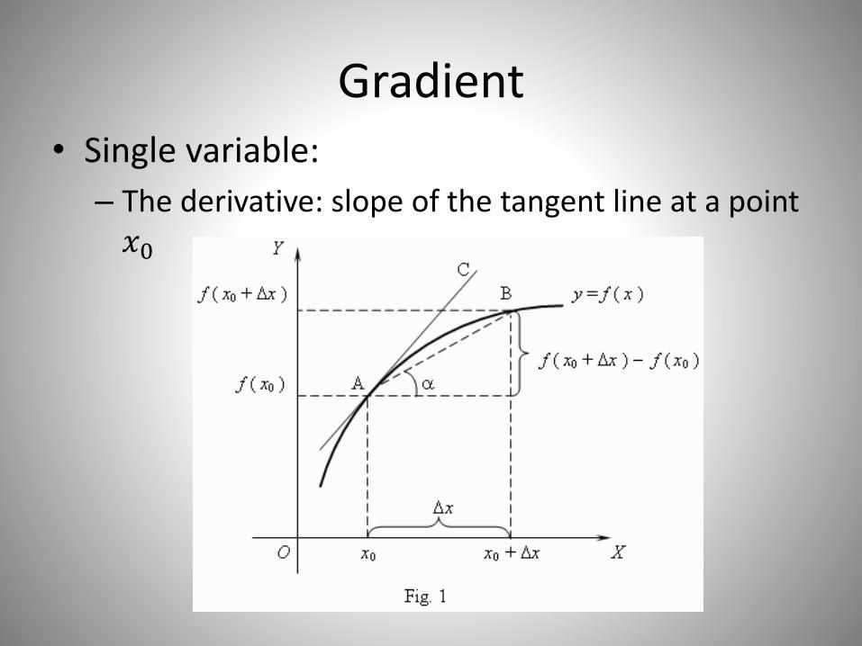
Gradient• Single variable:

– The derivative: slope of the tangent line at a point 𝑥0

Gradient• Multivariable:

– 𝛻𝑓 =𝜕𝑓

𝜕𝑥1,𝜕𝑓

𝜕𝑥2, … ,

𝜕𝑓

𝜕𝑥𝑛

– A vector of partial derivatives with respect to each of the independent variables

• 𝛻𝑓 points in the direction of greatest rate of change or “steepest ascent”

• Magnitude (or length) of 𝛻𝑓 is the greatest rate of change

Gradient

The general idea

• We have k parameters 𝜃1, 𝜃2, … , 𝜃𝑘we’d like to train for a model – with respect to some error/loss function 𝐽(𝜃1, … , 𝜃𝑘) to be minimized

• Gradient descent is one way to iteratively determine the optimal set of parameter values:

1. Initialize parameters

2. Keep changing values to reduce 𝐽(𝜃1, … , 𝜃𝑘)

– 𝛻𝐽 tells us which direction increases 𝐽 the most

– We go in the opposite direction of 𝛻𝐽

To actually descend…

Set initial parameter values 𝜃10, … , 𝜃𝑘

0

while(not converged) {

calculate 𝛻𝐽 (i.e. evaluate 𝜕𝐽

𝜕𝜃1, … ,

𝜕𝐽

𝜕𝜃𝑘)

do {

𝜃1 ≔ 𝜃1 − α𝜕𝐽

𝜕𝜃1

𝜃2 ≔ 𝜃2 − α𝜕𝐽

𝜕𝜃2

⋮𝜃𝑘 ≔ 𝜃𝑘 − α

𝜕𝐽

𝜕𝜃𝑘}

}

Where α is the ‘learning rate’ or ‘step size’

- Small enough α ensures 𝐽 𝜃1𝑖 , … , 𝜃𝑘

𝑖 ≤ 𝐽(𝜃1𝑖−1, … , 𝜃𝑘

𝑖−1)

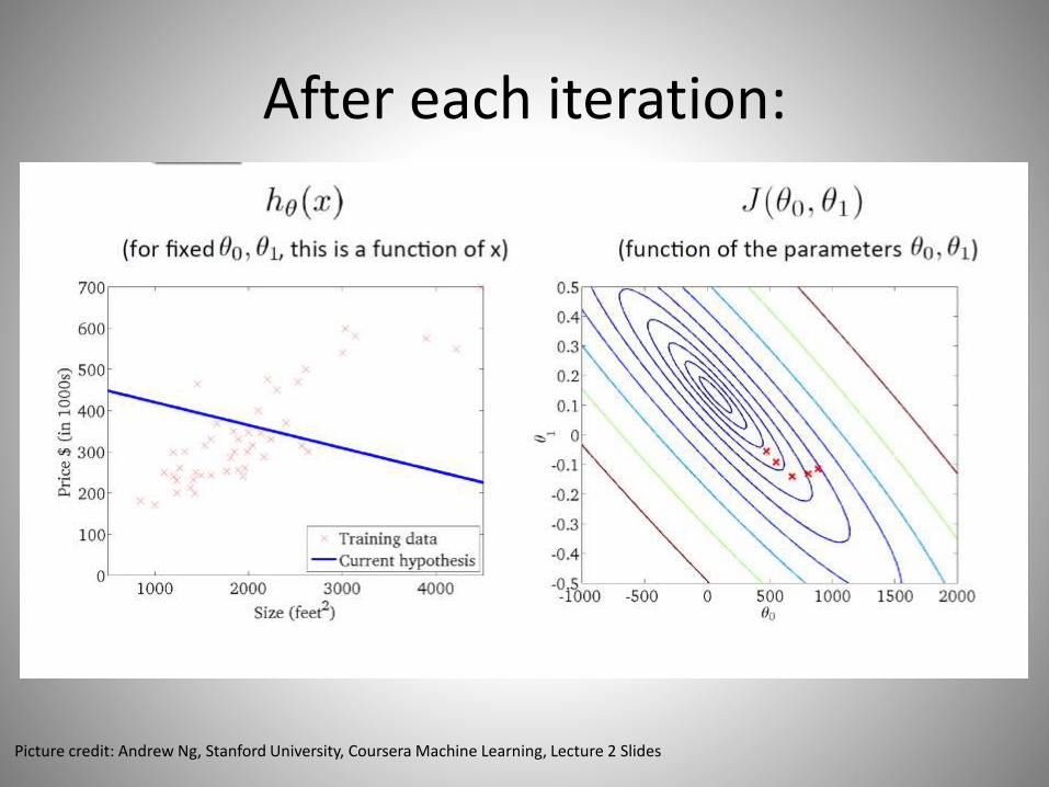
After each iteration:

Picture credit: Andrew Ng, Stanford University, Coursera Machine Learning, Lecture 2 Slides

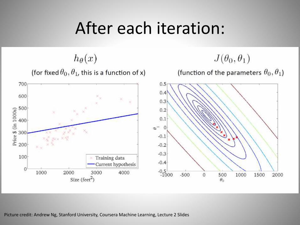
After each iteration:

Picture credit: Andrew Ng, Stanford University, Coursera Machine Learning, Lecture 2 Slides

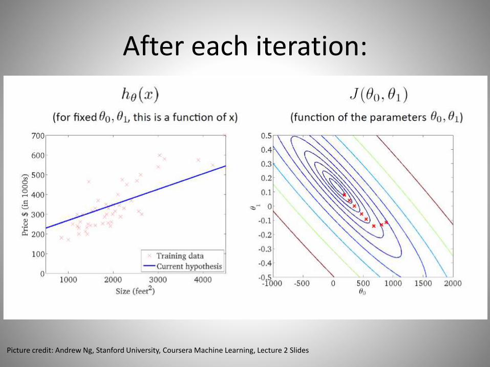
After each iteration:

Picture credit: Andrew Ng, Stanford University, Coursera Machine Learning, Lecture 2 Slides

After each iteration:

Picture credit: Andrew Ng, Stanford University, Coursera Machine Learning, Lecture 2 Slides

After each iteration:

Picture credit: Andrew Ng, Stanford University, Coursera Machine Learning, Lecture 2 Slides

After each iteration:

Picture credit: Andrew Ng, Stanford University, Coursera Machine Learning, Lecture 2 Slides

After each iteration:

Picture credit: Andrew Ng, Stanford University, Coursera Machine Learning, Lecture 2 Slides

After each iteration:

Picture credit: Andrew Ng, Stanford University, Coursera Machine Learning, Lecture 2 Slides

Issues

• Convex objective function guarantees convergence to global minimum

• Non-convexity brings the possibility of getting stuck in a local minimum

– Different, randomized starting values can fight this

Initial Values and Convergence

Picture credit: Andrew Ng, Stanford University, Coursera Machine Learning, Lecture 2 Slides

Initial Values and Convergence

Picture credit: Andrew Ng, Stanford University, Coursera Machine Learning, Lecture 2 Slides

Issues cont.

• Convergence can be slow

– Larger learning rate α can speed things up, but with too large of α, optimums can be ‘jumped’ or skipped over - requiring more iterations

– Too small of a step size will keep convergence slow

– Can be combined with a line search to find the optimal α on every iteration