Learning to learn by gradient descentby gradient descent

Marcin Andrychowicz1, Misha Denil1, Sergio Gómez Colmenarejo1, Matthew W. Hoffman1,David Pfau1, Tom Schaul1, Brendan Shillingford1,2, Nando de Freitas1,2,3

1Google DeepMind 2University of Oxford 3Canadian Institute for Advanced Research

marcin.andrychowicz@gmail.com

{mdenil,sergomez,mwhoffman,pfau,schaul}@google.com

brendan.shillingford@cs.ox.ac.uk, nandodefreitas@google.com

Abstract

The move from hand-designed features to learned features in machine learning hasbeen wildly successful. In spite of this, optimization algorithms are still designedby hand. In this paper we show how the design of an optimization algorithm can becast as a learning problem, allowing the algorithm to learn to exploit structure inthe problems of interest in an automatic way. Our learned algorithms, implementedby LSTMs, outperform generic, hand-designed competitors on the tasks for whichthey are trained, and also generalize well to new tasks with similar structure. Wedemonstrate this on a number of tasks, including simple convex problems, trainingneural networks, and styling images with neural art.

1 Introduction

Frequently, tasks in machine learning can be expressed as the problem of optimizing an objectivefunction f(✓) defined over some domain ✓ 2 ⇥. The goal in this case is to find the minimizer✓

⇤= argmin✓2⇥

f(✓). While any method capable of minimizing this objective function can beapplied, the standard approach for differentiable functions is some form of gradient descent, resultingin a sequence of updates

✓t+1

= ✓t � ↵trf(✓t) .

The performance of vanilla gradient descent, however, is hampered by the fact that it only makes useof gradients and ignores second-order information. Classical optimization techniques correct thisbehavior by rescaling the gradient step using curvature information, typically via the Hessian matrixof second-order partial derivatives—although other choices such as the generalized Gauss-Newtonmatrix or Fisher information matrix are possible.

Much of the modern work in optimization is based around designing update rules tailored to specificclasses of problems, with the types of problems of interest differing between different researchcommunities. For example, in the deep learning community we have seen a proliferation of optimiza-tion methods specialized for high-dimensional, non-convex optimization problems. These includemomentum [Nesterov, 1983, Tseng, 1998], Rprop [Riedmiller and Braun, 1993], Adagrad [Duchiet al., 2011], RMSprop [Tieleman and Hinton, 2012], and ADAM [Kingma and Ba, 2015]. Morefocused methods can also be applied when more structure of the optimization problem is known[Martens and Grosse, 2015]. In contrast, communities who focus on sparsity tend to favor verydifferent approaches [Donoho, 2006, Bach et al., 2012]. This is even more the case for combinatorialoptimization for which relaxations are often the norm [Nemhauser and Wolsey, 1988].

30th Conference on Neural Information Processing Systems (NIPS 2016), Barcelona, Spain.

optimizer optimizee

parameter updates

error signal

Figure 1: The optimizer (left) is provided withperformance of the optimizee (right) and proposesupdates to increase the optimizee’s performance.[photos: Bobolas, 2009, Maley, 2011]

This industry of optimizer design allows differ-ent communities to create optimization meth-ods which exploit structure in their problemsof interest at the expense of potentially poorperformance on problems outside of that scope.Moreover the No Free Lunch Theorems for Op-timization [Wolpert and Macready, 1997] showthat in the setting of combinatorial optimization,no algorithm is able to do better than a randomstrategy in expectation. This suggests that spe-cialization to a subclass of problems is in factthe only way that improved performance can beachieved in general.

In this work we take a different tack and insteadpropose to replace hand-designed update ruleswith a learned update rule, which we call the op-timizer g, specified by its own set of parameters�. This results in updates to the optimizee f ofthe form

✓t+1

= ✓t + gt(rf(✓t),�) . (1)A high level view of this process is shown in Figure 1. In what follows we will explicitly modelthe update rule g using a recurrent neural network (RNN) which maintains its own state and hencedynamically updates as a function of its iterates.

1.1 Transfer learning and generalization

The goal of this work is to develop a procedure for constructing a learning algorithm which performswell on a particular class of optimization problems. Casting algorithm design as a learning problemallows us to specify the class of problems we are interested in through example problem instances.This is in contrast to the ordinary approach of characterizing properties of interesting problemsanalytically and using these analytical insights to design learning algorithms by hand.

It is informative to consider the meaning of generalization in this framework. In ordinary statisticallearning we have a particular function of interest, whose behavior is constrained through a data set ofexample function evaluations. In choosing a model we specify a set of inductive biases about howwe think the function of interest should behave at points we have not observed, and generalizationcorresponds to the capacity to make predictions about the behavior of the target function at novelpoints. In our setting the examples are themselves problem instances, which means generalizationcorresponds to the ability to transfer knowledge between different problems. This reuse of problemstructure is commonly known as transfer learning, and is often treated as a subject in its own right.However, by taking a meta-learning perspective, we can cast the problem of transfer learning as oneof generalization, which is much better studied in the machine learning community.

One of the great success stories of deep-learning is that we can rely on the ability of deep networks togeneralize to new examples by learning interesting sub-structures. In this work we aim to leveragethis generalization power, but also to lift it from simple supervised learning to the more generalsetting of optimization.

1.2 A brief history and related work

The idea of using learning to learn or meta-learning to acquire knowledge or inductive biases has along history [Thrun and Pratt, 1998]. More recently, Lake et al. [2016] have argued forcefully forits importance as a building block in artificial intelligence. Similarly, Santoro et al. [2016] framemulti-task learning as generalization, however unlike our approach they directly train a base learnerrather than a training algorithm. In general these ideas involve learning which occurs at two differenttime scales: rapid learning within tasks and more gradual, meta learning across many different tasks.

Perhaps the most general approach to meta-learning is that of Schmidhuber [1992, 1993]—buildingon work from [Schmidhuber, 1987]—which considers networks that are able to modify their ownweights. Such a system is differentiable end-to-end, allowing both the network and the learning

2

algorithm to be trained jointly by gradient descent with few restrictions. However this generalitycomes at the expense of making the learning rules very difficult to train. Alternatively, the workof Schmidhuber et al. [1997] uses the Success Story Algorithm to modify its search strategy ratherthan gradient descent; a similar approach has been recently taken in Daniel et al. [2016] which usesreinforcement learning to train a controller for selecting step-sizes.

Bengio et al. [1990, 1995] propose to learn updates which avoid back-propagation by using simpleparametric rules. In relation to the focus of this paper the work of Bengio et al. could be characterizedas learning to learn without gradient descent by gradient descent. The work of Runarsson andJonsson [2000] builds upon this work by replacing the simple rule with a neural network.

Cotter and Conwell [1990], and later Younger et al. [1999], also show fixed-weight recurrent neuralnetworks can exhibit dynamic behavior without need to modify their network weights. Similarly thishas been shown in a filtering context [e.g. Feldkamp and Puskorius, 1998], which is directly relatedto simple multi-timescale optimizers [Sutton, 1992, Schraudolph, 1999].

Finally, the work of Younger et al. [2001] and Hochreiter et al. [2001] connects these different threadsof research by allowing for the output of backpropagation from one network to feed into an additionallearning network, with both networks trained jointly. Our approach to meta-learning builds on thiswork by modifying the network architecture of the optimizer in order to scale this approach to largerneural-network optimization problems.

2 Learning to learn with recurrent neural networks

In this work we consider directly parameterizing the optimizer. As a result, in a slight abuse of notationwe will write the final optimizee parameters ✓⇤(f,�) as a function of the optimizer parameters � andthe function in question. We can then ask the question: What does it mean for an optimizer to begood? Given a distribution of functions f we will write the expected loss as

L(�) = Ef

hf

�✓

⇤(f,�)

�i. (2)

As noted earlier, we will take the update steps gt to be the output of a recurrent neural network m,parameterized by �, whose state we will denote explicitly with ht. Next, while the objective functionin (2) depends only on the final parameter value, for training the optimizer it will be convenient tohave an objective that depends on the entire trajectory of optimization, for some horizon T,

L(�) = Ef

"TX

t=1

wtf(✓t)

#where ✓t+1

= ✓t + gt ,gt

ht+1

�= m(rt, ht,�) .

(3)

Here wt 2 R�0

are arbitrary weights associated with each time-step and we will also use the notationrt = r✓f(✓t). This formulation is equivalent to (2) when wt = 1[t = T ], but later we will describewhy using different weights can prove useful.

We can minimize the value of L(�) using gradient descent on �. The gradient estimate @L(�)/@� canbe computed by sampling a random function f and applying backpropagation to the computationalgraph in Figure 2. We allow gradients to flow along the solid edges in the graph, but gradientsalong the dashed edges are dropped. Ignoring gradients along the dashed edges amounts to makingthe assumption that the gradients of the optimizee do not depend on the optimizer parameters, i.e.@rt

�@� = 0. This assumption allows us to avoid computing second derivatives of f .

Examining the objective in (3) we see that the gradient is non-zero only for terms where wt 6= 0. Ifwe use wt = 1[t = T ] to match the original problem, then gradients of trajectory prefixes are zeroand only the final optimization step provides information for training the optimizer. This rendersBackpropagation Through Time (BPTT) inefficient. We solve this problem by relaxing the objectivesuch that wt > 0 at intermediate points along the trajectory. This changes the objective function, butallows us to train the optimizer on partial trajectories. For simplicity, in all our experiments we usewt = 1 for every t.

3

Optimizee

Optimizer

t-2 t-1 t

m m m

+ + +

ft-1 ftft-2

∇t-2 ∇t-1 ∇t

ht-2 ht-1 ht ht+1

gt-1 gt

θt-2 θt-1 θt θt+1

gt-2

Figure 2: Computational graph used for computing the gradient of the optimizer.

2.1 Coordinatewise LSTM optimizer

One challenge in applying RNNs in our setting is that we want to be able to optimize at least tens ofthousands of parameters. Optimizing at this scale with a fully connected RNN is not feasible as itwould require a huge hidden state and an enormous number of parameters. To avoid this difficulty wewill use an optimizer m which operates coordinatewise on the parameters of the objective function,similar to other common update rules like RMSprop and ADAM. This coordinatewise networkarchitecture allows us to use a very small network that only looks at a single coordinate to define theoptimizer and share optimizer parameters across different parameters of the optimizee.

Different behavior on each coordinate is achieved by using separate activations for each objectivefunction parameter. In addition to allowing us to use a small network for this optimizer, this setup hasthe nice effect of making the optimizer invariant to the order of parameters in the network, since thesame update rule is used independently on each coordinate.

LSTM1

f

LSTMn

∇1

θ1

θn

+

+

…

∇n

…… ……

Figure 3: One step of an LSTM optimizer. AllLSTMs have shared parameters, but separate hid-den states.

We implement the update rule for each coordi-nate using a two-layer Long Short Term Memory(LSTM) network [Hochreiter and Schmidhuber,1997], using the now-standard forget gate archi-tecture. The network takes as input the opti-mizee gradient for a single coordinate as wellas the previous hidden state and outputs the up-date for the corresponding optimizee parameter.We will refer to this architecture, illustrated inFigure 3, as an LSTM optimizer.

The use of recurrence allows the LSTM to learndynamic update rules which integrate informa-tion from the history of gradients, similar tomomentum. This is known to have many desir-able properties in convex optimization [see e.g.Nesterov, 1983] and in fact many recent learning procedures—such as ADAM—use momentum intheir updates.

Preprocessing and postprocessing Optimizer inputs and outputs can have very different magni-tudes depending on the class of function being optimized, but neural networks usually work robustlyonly for inputs and outputs which are neither very small nor very large. In practice rescaling inputsand outputs of an LSTM optimizer using suitable constants (shared across all timesteps and functionsf ) is sufficient to avoid this problem. In Appendix A we propose a different method of preprocessinginputs to the optimizer inputs which is more robust and gives slightly better performance.

4

Figure 4: Comparisons between learned and hand-crafted optimizers performance. Learned optimiz-ers are shown with solid lines and hand-crafted optimizers are shown with dashed lines. Units for they axis in the MNIST plots are logits. Left: Performance of different optimizers on randomly sampled10-dimensional quadratic functions. Center: the LSTM optimizer outperforms standard methodstraining the base network on MNIST. Right: Learning curves for steps 100-200 by an optimizertrained to optimize for 100 steps (continuation of center plot).

3 Experiments

In all experiments the trained optimizers use two-layer LSTMs with 20 hidden units in each layer.Each optimizer is trained by minimizing Equation 3 using truncated BPTT as described in Section 2.The minimization is performed using ADAM with a learning rate chosen by random search.

We use early stopping when training the optimizer in order to avoid overfitting the optimizer. Aftereach epoch (some fixed number of learning steps) we freeze the optimizer parameters and evaluate itsperformance. We pick the best optimizer (according to the final validation loss) and report its averageperformance on a number of freshly sampled test problems.

We compare our trained optimizers with standard optimizers used in Deep Learning: SGD, RMSprop,ADAM, and Nesterov’s accelerated gradient (NAG). For each of these optimizer and each problemwe tuned the learning rate, and report results with the rate that gives the best final error for eachproblem. When an optimizer has more parameters than just a learning rate (e.g. decay coefficients forADAM) we use the default values from the optim package in Torch7. Initial values of all optimizeeparameters were sampled from an IID Gaussian distribution.

3.1 Quadratic functions

In this experiment we consider training an optimizer on a simple class of synthetic 10-dimensionalquadratic functions. In particular we consider minimizing functions of the form

f(✓) = kW✓ � yk22

for different 10x10 matrices W and 10-dimensional vectors y whose elements are drawn from an IIDGaussian distribution. Optimizers were trained by optimizing random functions from this family andtested on newly sampled functions from the same distribution. Each function was optimized for 100steps and the trained optimizers were unrolled for 20 steps. We have not used any preprocessing, norpostprocessing.

Learning curves for different optimizers, averaged over many functions, are shown in the left plot ofFigure 4. Each curve corresponds to the average performance of one optimization algorithm on manytest functions; the solid curve shows the learned optimizer performance and dashed curves showthe performance of the standard baseline optimizers. It is clear the learned optimizers substantiallyoutperform the baselines in this setting.

3.2 Training a small neural network on MNIST

In this experiment we test whether trainable optimizers can learn to optimize a small neural networkon MNIST, and also explore how the trained optimizers generalize to functions beyond those theywere trained on. To this end, we train the optimizer to optimize a base network and explore a seriesof modifications to the network architecture and training procedure at test time.

5

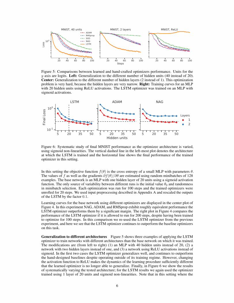
Figure 5: Comparisons between learned and hand-crafted optimizers performance. Units for they axis are logits. Left: Generalization to the different number of hidden units (40 instead of 20).Center: Generalization to the different number of hidden layers (2 instead of 1). This optimizationproblem is very hard, because the hidden layers are very narrow. Right: Training curves for an MLPwith 20 hidden units using ReLU activations. The LSTM optimizer was trained on an MLP withsigmoid activations.

Figure 6: Systematic study of final MNIST performance as the optimizee architecture is varied,using sigmoid non-linearities. The vertical dashed line in the left-most plot denotes the architectureat which the LSTM is trained and the horizontal line shows the final performance of the trainedoptimizer in this setting.

In this setting the objective function f(✓) is the cross entropy of a small MLP with parameters ✓.The values of f as well as the gradients @f(✓)/@✓ are estimated using random minibatches of 128examples. The base network is an MLP with one hidden layer of 20 units using a sigmoid activationfunction. The only source of variability between different runs is the initial value ✓

0

and randomnessin minibatch selection. Each optimization was run for 100 steps and the trained optimizers wereunrolled for 20 steps. We used input preprocessing described in Appendix A and rescaled the outputsof the LSTM by the factor 0.1.

Learning curves for the base network using different optimizers are displayed in the center plot ofFigure 4. In this experiment NAG, ADAM, and RMSprop exhibit roughly equivalent performance theLSTM optimizer outperforms them by a significant margin. The right plot in Figure 4 compares theperformance of the LSTM optimizer if it is allowed to run for 200 steps, despite having been trainedto optimize for 100 steps. In this comparison we re-used the LSTM optimizer from the previousexperiment, and here we see that the LSTM optimizer continues to outperform the baseline optimizerson this task.

Generalization to different architectures Figure 5 shows three examples of applying the LSTMoptimizer to train networks with different architectures than the base network on which it was trained.The modifications are (from left to right) (1) an MLP with 40 hidden units instead of 20, (2) anetwork with two hidden layers instead of one, and (3) a network using ReLU activations instead ofsigmoid. In the first two cases the LSTM optimizer generalizes well, and continues to outperformthe hand-designed baselines despite operating outside of its training regime. However, changingthe activation function to ReLU makes the dynamics of the learning procedure sufficiently differentthat the learned optimizer is no longer able to generalize. Finally, in Figure 6 we show the resultsof systematically varying the tested architecture; for the LSTM results we again used the optimizertrained using 1 layer of 20 units and sigmoid non-linearities. Note that in this setting where the

6

Figure 7: Optimization performance on the CIFAR-10 dataset and subsets. Shown on the left is theLSTM optimizer versus various baselines trained on CIFAR-10 and tested on a held-out test set. Thetwo plots on the right are the performance of these optimizers on subsets of the CIFAR labels. Theadditional optimizer LSTM-sub has been trained only on the heldout labels and is hence transferringto a completely novel dataset.

test-set problems are similar enough to those in the training set we see even better generalization thanthe baseline optimizers.

3.3 Training a convolutional network on CIFAR-10

Next we test the performance of the trained neural optimizers on optimizing classification performancefor the CIFAR-10 dataset [Krizhevsky, 2009]. In these experiments we used a model with bothconvolutional and feed-forward layers. In particular, the model used for these experiments includesthree convolutional layers with max pooling followed by a fully-connected layer with 32 hidden units;all non-linearities were ReLU activations with batch normalization.

The coordinatewise network decomposition introduced in Section 2.1—and used in the previousexperiment—utilizes a single LSTM architecture with shared weights, but separate hidden states,for each optimizee parameter. We found that this decomposition was not sufficient for the modelarchitecture introduced in this section due to the differences between the fully connected and convo-lutional layers. Instead we modify the optimizer by introducing two LSTMs: one proposes parameterupdates for the fully connected layers and the other updates the convolutional layer parameters. Likethe previous LSTM optimizer we still utilize a coordinatewise decomposition with shared weightsand individual hidden states, however LSTM weights are now shared only between parameters of thesame type (i.e. fully-connected vs. convolutional).

The performance of this trained optimizer compared against the baseline techniques is shown inFigure 7. The left-most plot displays the results of using the optimizer to fit a classifier on a held-outtest set. The additional two plots on the right display the performance of the trained optimizer onmodified datasets which only contain a subset of the labels, i.e. the CIFAR-2 dataset only containsdata corresponding to 2 of the 10 labels. Additionally we include an optimizer LSTM-sub which wasonly trained on the held-out labels.

In all these examples we can see that the LSTM optimizer learns much more quickly than the baselineoptimizers, with significant boosts in performance for the CIFAR-5 and especially CIFAR-2 datsets.We also see that the optimizers trained only on a disjoint subset of the data is hardly effected by thisdifference and transfers well to the additional dataset.

3.4 Neural Art

The recent work on artistic style transfer using convolutional networks, or Neural Art [Gatys et al.,2015], gives a natural testbed for our method, since each content and style image pair gives rise to adifferent optimization problem. Each Neural Art problem starts from a content image, c, and a styleimage, s, and is given by

f(✓) = ↵Lcontent

(c, ✓) + �Lstyle

(s, ✓) + �Lreg

(✓)

The minimizer of f is the styled image. The first two terms try to match the content and style ofthe styled image to that of their first argument, and the third term is a regularizer that encouragessmoothness in the styled image. Details can be found in [Gatys et al., 2015].

7

Figure 8: Optimization curves for Neural Art. Content images come from the test set, which was notused during the LSTM optimizer training. Note: the y-axis is in log scale and we zoom in on theinteresting portion of this plot. Left: Applying the training style at the training resolution. Right:Applying the test style at double the training resolution.

Figure 9: Examples of images styled using the LSTM optimizer. Each triple consists of the contentimage (left), style (right) and image generated by the LSTM optimizer (center). Left: The result ofapplying the training style at the training resolution to a test image. Right: The result of applying anew style to a test image at double the resolution on which the optimizer was trained.

We train optimizers using only 1 style and 1800 content images taken from ImageNet [Deng et al.,2009]. We randomly select 100 content images for testing and 20 content images for validation oftrained optimizers. We train the optimizer on 64x64 content images from ImageNet and one fixedstyle image. We then test how well it generalizes to a different style image and higher resolution(128x128). Each image was optimized for 128 steps and trained optimizers were unrolled for 32steps. Figure 9 shows the result of styling two different images using the LSTM optimizer. TheLSTM optimizer uses inputs preprocessing described in Appendix A and no postprocessing. SeeAppendix C for additional images.

Figure 8 compares the performance of the LSTM optimizer to standard optimization algorithms. TheLSTM optimizer outperforms all standard optimizers if the resolution and style image are the sameas the ones on which it was trained. Moreover, it continues to perform very well when both theresolution and style are changed at test time.

Finally, in Appendix B we qualitatively examine the behavior of the step directions generated by thelearned optimizer.

4 Conclusion

We have shown how to cast the design of optimization algorithms as a learning problem, whichenables us to train optimizers that are specialized to particular classes of functions. Our experimentshave confirmed that learned neural optimizers compare favorably against state-of-the-art optimizationmethods used in deep learning. We witnessed a remarkable degree of transfer, with for example theLSTM optimizer trained on 12,288 parameter neural art tasks being able to generalize to tasks with49,152 parameters, different styles, and different content images all at the same time. We observedsimilar impressive results when transferring to different architectures in the MNIST task.

The results on the CIFAR image labeling task show that the LSTM optimizers outperform hand-engineered optimizers when transferring to datasets drawn from the same data distribution.

ReferencesF. Bach, R. Jenatton, J. Mairal, and G. Obozinski. Optimization with sparsity-inducing penalties. Foundations

and Trends in Machine Learning, 4(1):1–106, 2012.

8

S. Bengio, Y. Bengio, and J. Cloutier. On the search for new learning rules for ANNs. Neural Processing Letters,2(4):26–30, 1995.

Y. Bengio, S. Bengio, and J. Cloutier. Learning a synaptic learning rule. Université de Montréal, Départementd’informatique et de recherche opérationnelle, 1990.

F. Bobolas. brain-neurons, 2009. URL https://www.flickr.com/photos/fbobolas/3822222947. Cre-ative Commons Attribution-ShareAlike 2.0 Generic.

N. E. Cotter and P. R. Conwell. Fixed-weight networks can learn. In International Joint Conference on NeuralNetworks, pages 553–559, 1990.

C. Daniel, J. Taylor, and S. Nowozin. Learning step size controllers for robust neural network training. InAssociation for the Advancement of Artificial Intelligence, 2016.

J. Deng, W. Dong, R. Socher, L.-J. Li, K. Li, and L. Fei-Fei. Imagenet: A large-scale hierarchical image database.In Computer Vision and Pattern Recognition, pages 248–255. IEEE, 2009.

D. L. Donoho. Compressed sensing. Transactions on Information Theory, 52(4):1289–1306, 2006.J. Duchi, E. Hazan, and Y. Singer. Adaptive subgradient methods for online learning and stochastic optimization.

Journal of Machine Learning Research, 12:2121–2159, 2011.L. A. Feldkamp and G. V. Puskorius. A signal processing framework based on dynamic neural networks

with application to problems in adaptation, filtering, and classification. Proceedings of the IEEE, 86(11):2259–2277, 1998.

L. A. Gatys, A. S. Ecker, and M. Bethge. A neural algorithm of artistic style. arXiv Report 1508.06576, 2015.S. Hochreiter and J. Schmidhuber. Long short-term memory. Neural computation, 9(8):1735–1780, 1997.S. Hochreiter, A. S. Younger, and P. R. Conwell. Learning to learn using gradient descent. In International

Conference on Artificial Neural Networks, pages 87–94. Springer, 2001.D. P. Kingma and J. Ba. Adam: A method for stochastic optimization. In International Conference on Learning

Representations, 2015.A. Krizhevsky. Learning multiple layers of features from tiny images. Technical report, 2009.B. M. Lake, T. D. Ullman, J. B. Tenenbaum, and S. J. Gershman. Building machines that learn and think like

people. arXiv Report 1604.00289, 2016.T. Maley. neuron, 2011. URL https://www.flickr.com/photos/taylortotz101/6280077898. Creative

Commons Attribution 2.0 Generic.J. Martens and R. Grosse. Optimizing neural networks with Kronecker-factored approximate curvature. In

International Conference on Machine Learning, pages 2408–2417, 2015.G. L. Nemhauser and L. A. Wolsey. Integer and combinatorial optimization. John Wiley & Sons, 1988.Y. Nesterov. A method of solving a convex programming problem with convergence rate o (1/k2). In Soviet

Mathematics Doklady, volume 27, pages 372–376, 1983.M. Riedmiller and H. Braun. A direct adaptive method for faster backpropagation learning: The RPROP

algorithm. In International Conference on Neural Networks, pages 586–591, 1993.T. P. Runarsson and M. T. Jonsson. Evolution and design of distributed learning rules. In IEEE Symposium on

Combinations of Evolutionary Computation and Neural Networks, pages 59–63. IEEE, 2000.A. Santoro, S. Bartunov, M. Botvinick, D. Wierstra, and T. Lillicrap. Meta-learning with memory-augmented

neural networks. In International Conference on Machine Learning, 2016.J. Schmidhuber. Evolutionary principles in self-referential learning; On learning how to learn: The meta-meta-...

hook. PhD thesis, Institut f. Informatik, Tech. Univ. Munich, 1987.J. Schmidhuber. Learning to control fast-weight memories: An alternative to dynamic recurrent networks.

Neural Computation, 4(1):131–139, 1992.J. Schmidhuber. A neural network that embeds its own meta-levels. In International Conference on Neural

Networks, pages 407–412. IEEE, 1993.J. Schmidhuber, J. Zhao, and M. Wiering. Shifting inductive bias with success-story algorithm, adaptive levin

search, and incremental self-improvement. Machine Learning, 28(1):105–130, 1997.N. N. Schraudolph. Local gain adaptation in stochastic gradient descent. In International Conference on

Artificial Neural Networks, volume 2, pages 569–574, 1999.R. S. Sutton. Adapting bias by gradient descent: An incremental version of delta-bar-delta. In Association for

the Advancement of Artificial Intelligence, pages 171–176, 1992.S. Thrun and L. Pratt. Learning to learn. Springer Science & Business Media, 1998.T. Tieleman and G. Hinton. Lecture 6.5-rmsprop: Divide the gradient by a running average of its recent

magnitude. COURSERA: Neural Networks for Machine Learning, 4:2, 2012.P. Tseng. An incremental gradient (-projection) method with momentum term and adaptive stepsize rule. Journal

on Optimization, 8(2):506–531, 1998.D. H. Wolpert and W. G. Macready. No free lunch theorems for optimization. Transactions on Evolutionary

Computation, 1(1):67–82, 1997.A. S. Younger, P. R. Conwell, and N. E. Cotter. Fixed-weight on-line learning. Transactions on Neural Networks,

10(2):272–283, 1999.A. S. Younger, S. Hochreiter, and P. R. Conwell. Meta-learning with backpropagation. In International Joint

Conference on Neural Networks, 2001.

9