Optimization of Rib-to-Deck Welds for Steel Orthotropic ... · PDF fileOptimization of...

Optimization of Rib-to-Deck Welds forSteel Orthotropic Bridge Decks

PUBLICATION NO. FHWA-HRT-17-020 FEBRUARY 2017

Research, Development, and TechnologyTurner-Fairbank Highway Research Center6300 Georgetown PikeMcLean, VA 22101-2296

FOREWORD

This report documents fatigue testing results of full-scale geometries of various orthotropic rib-to-deck weld geometries. The Federal Highway Administration undertook this study in order to assess these weld geometries and potentially provide performance data that might alleviate restrictive fabrication specifications. Currently, these restrictions are reducing the competitiveness of orthotropic steel decks versus other alternatives. Parameters explored in the research were welding process, weld penetration, and fit-up tolerance. The results showed that fatigue resistance could be assured in design through simple fabrication rules that define the weld leg size and target penetration and, if implemented, should make rib-to-deck welds more fabricator-friendly to produce while still maintaining reliability against fatigue failures.

This report will benefit those interested in the design and fabrication of steel orthotropic bridge decks, including State transportation departments, steel bridge fabricators, design consultants, and researchers.

Cheryl Richter Director, Office of Infrastructure Research and Development

Notice This document is disseminated under the sponsorship of the U.S. Department of Transportation in the interest of information exchange. The U.S. Government assumes no liability for the use of the information contained in this document. The U.S. Government does not endorse products or manufacturers. Trademarks or manufacturers’ names appear in this report only because they are considered essential to the objective of the document.

Quality Assurance Statement The Federal Highway Administration (FHWA) provides high-quality information to serve Government, industry, and the public in a manner that promotes public understanding. Standards and policies are used to ensure and maximize the quality, objectivity, utility, and integrity of its information. FHWA periodically reviews quality issues and adjusts its programs and processes to ensure continuous quality improvement.

TECHNICAL REPORT DOCUMENTATION PAGE 1. Report No. FHWA-HRT-17-020

2. Government Accession No.

3. Recipient’s Catalog No.

4. Title and Subtitle Optimization of Rib-to-Deck Welds for Steel Orthotropic Bridge Decks

5. Report Date February 2017 6. Performing Organization Code:

7. Author(s) J.M. Ocel, B. Cross, W.J. Wright, and H. Yuan

8. Performing Organization Report No.

9. Performing Organization Name and Address Office of Infrastructure Research & Development Federal Highway Administration 6300 Georgetown Pike McLean, VA 22101-2296 Virginia Polytechnic Institute and State University Civil and Environmental Engineering Department 1880 Pratt Drive Blacksburg, VA 24060-6343

10. Work Unit No. 11. Contract or Grant No. DTFH61-04-C-00029 including Task Orders 28–30 DTFH061-10-D-00017 including Task Order 2

12. Sponsoring Agency Name and Address Office of Infrastructure Research and Development Federal Highway Administration 6300 Georgetown Pike McLean, VA 22101-2296

13. Type of Report and Period Covered Final Report, October 2009–July 2012 14. Sponsoring Agency Code HRDI-40

15. Supplementary Notes Justin Ocel (HRDI-40) conducted the testing at Turner-Fairbank Highway Research Center, was the technical monitor of all task orders, and prepared the final report with assistance from onsite contractor staff under both contracts. The Contracting Officer’s Representative for both contracts was Fassil Beshah (HRDI-40). 16. Abstract Orthotropic steel decks have been widely used over the decades, especially on long-span bridges as a result of their lightweight and fast construction. However, fatigue cracking problems have been observed in the welds in many cases because of wheel loads. The rib-to-deck welds need special care because they are directly located under wheel loads and are subjected to both local and global stress effects.

When this research began, the current practice in the United States was to use a one-sided partial penetration weld joining the rib and deck plates together with a minimum of 80-percent penetration requirement. Melt-through and blow were also considered rejectable defects. Restrictive requirements such as these result in a very narrowly defined welding procedure with little tolerance for variation. In practice, this leads to numerous weld repairs and rigorous inspection requirements that drive up the cost of orthotropic deck fabrication.

This study shows that the 80-percent penetration requirement can be significantly relaxed because fatigue performance was largely dictated by weld size and not penetration. A simple correlation is provided between weld size and penetration to guarantee American Association of State and Highway Transportation Officials category C fatigue performance that should provide for more relaxed fabrication specifications. Finally, specimens fabricated with purposeful fit-up gaps were found to close provided the original gap did not exceed 0.020 inch. 17. Key Words Local structural stress, steel bridge, orthotropic steel deck, fatigue testing

18. Distribution Statement No restrictions. This document is available through the National Technical Information Service, Springfield, VA 22161. http://www.ntis.gov

19. Security Classif. (of this report) Unclassified

20. Security Classif. (of this page) Unclassified

21. No. of Pages 121

22. Price N/A

Form DOT F 1700.7 (8-72) Reproduction of completed page authorized.

iii

TABLE OF CONTENTS

INTRODUCTION......................................................................................................................... 1 BACKGROUND ....................................................................................................................... 1 OBJECTIVES ........................................................................................................................... 2 APPROACH .............................................................................................................................. 3

EXPERIMENTAL STUDY ......................................................................................................... 5 SPECIMEN FABRICATION .................................................................................................. 5 TEST MATRIX ......................................................................................................................... 8 TEST SETUP AND PROCEDURE ...................................................................................... 14

Test Setup .............................................................................................................................. 14 Test Procedure ...................................................................................................................... 17

LSS ANALYSIS .......................................................................................................................... 19

RESULTS .................................................................................................................................... 25 ROOT CONDITION .............................................................................................................. 38 FATIGUE RESULTS ............................................................................................................. 40

REGRESSION ANALYSIS OF FATIGUE RESULTS .......................................................... 47 STATISTICAL DATASET .................................................................................................... 47

Regression Function .............................................................................................................. 48 Cross-Validation ................................................................................................................... 49 Standard Least Squares Linear Regression ........................................................................... 50

DESIGN RECOMMENDATIONS ....................................................................................... 55

CONCLUSIONS AND RECOMMENDATIONS .................................................................... 61 RECOMMENDATIONS........................................................................................................ 61 FUTURE RESEARCH ........................................................................................................... 62

APPENDIX A. SECTIONING OF PANELS INTO SPECIMENS........................................ 63

APPENDIX B. WELD DIMENSIONS ..................................................................................... 69

APPENDIX C. LASER WELD DIMENSIONS ..................................................................... 109

REFERENCES .......................................................................................................................... 113

iv

LIST OF FIGURES

Figure 1. Illustration. Typical closed-rib steel orthotropic deck panel ........................................... 2 Figure 2. Illustration. Type 1 rib geometry ..................................................................................... 6 Figure 3. Illustration. Type 2 rib geometry ..................................................................................... 7 Figure 4. Illustration. Type 3 rib geometry ..................................................................................... 8 Figure 5. Illustration. Comparison of rib edge preparation: beveled (left) and no

preparation (right) ................................................................................................................... 10 Figure 6. Illustration. Overbeveled (left) and underbeveled (right) edge preparation .................. 11 Figure 7. Photo. Typical saw cuts introduced at the weld roots on the OB and UB series

specimens ................................................................................................................................ 11 Figure 8. Illustration. Intentional fit-up gaps in OG1 panel (left) and OG2 panel (right) ............ 12 Figure 9. Illustration. Fit-up gap and edge preparation for W series ............................................ 13 Figure 10. Illustration. Test setup ................................................................................................. 15 Figure 11. Photo. Test setup at VT ............................................................................................... 16 Figure 12. Photo. Test setup at TFHRC ........................................................................................ 16 Figure 13. Illustration. Partitioning of specimen .......................................................................... 20 Figure 14. Illustration. Meshed specimen ..................................................................................... 21 Figure 15. Illustration. Membrane stress in specimen under unit load ......................................... 22 Figure 16. Illustration. Extrapolation points from rib and deck plate ........................................... 23 Figure 17. Photo. Macro of specimen SA4-2 (example of open root condition).......................... 38 Figure 18. Photo. Macro of specimen SA6-1 (example of closed root condition) ....................... 39 Figure 19. Photo. Macro of specimen W-1 ................................................................................... 39 Figure 20. Photo. Macro of specimen W-11 ................................................................................. 40 Figure 21. Graph. Plot of all R = −1 data ...................................................................................... 41 Figure 22. Graph. Plot of all R = 0 data ........................................................................................ 41 Figure 23. Graph. Plot of all root failures (R = −1) ...................................................................... 42 Figure 24. Graph. Plot of all R = 0 data sorted by penetration ..................................................... 43 Figure 25. Graph. Plot of all fatigue data differentiated by welding process ............................... 44 Figure 26. Graph. Relation between rib and deck plate leg sizes at R = −1 ................................. 45 Figure 27. Graph. Relation between rib and deck plate leg sizes at R = 0 ................................... 45 Figure 28. Graph. Relation between weld penetration and deck plate leg size at R = −1 ............ 45 Figure 29. Graph. Relation between weld penetration and deck plate leg size at R = 0 ............... 45 Figure 30. Graph. Relation between throat and deck plate leg sizes at R = −1 ............................ 46 Figure 31. Graph. Relation between throat and deck plate leg sizes at R = 0............................... 46 Figure 32. Graph. Relation between weld penetration and throat at R = −1 ................................ 46 Figure 33. Graph. Relation between weld penetration and throat at R = 0 ................................... 46 Figure 34. Equation. General regression function ........................................................................ 48 Figure 35. Equation. Linear regression function .......................................................................... 49 Figure 36. Equation. Standard least squares regression error function ......................................... 50 Figure 37. Graph. Standard regression cross-validation error ...................................................... 52 Figure 38. Equation. Least squares regression final predictive model ......................................... 54 Figure 39. Equation. Simplified least squares regression final predictive model ......................... 54 Figure 40. Graph. Normal probability plot of standard regression studentized residuals ............ 55 Figure 41. Histogram. Distribution of model residuals ................................................................ 56 Figure 42. Equation. Design fatigue resistance coefficient .......................................................... 56

v

Figure 43. Equation. Simplified design fatigue resistance coefficient ......................................... 56 Figure 44. Equation. Design weld-dimension inequality.............................................................. 57 Figure 45. Equation. Final design weld-dimension inequality ..................................................... 57 Figure 46. Scatterplot. Weld design inequality ............................................................................. 58 Figure 47. Histogram. Frequency of h-to-d1 ratio in experimental specimens ............................. 59 Figure 48. Illustration. Comparison of minimum weld dimensions for categories C or B

fatigue design .......................................................................................................................... 60 Figure 49. Illustration. GM8 series panel ..................................................................................... 63 Figure 50. Illustration. SA8 series panel ....................................................................................... 63 Figure 51. Illustration. SA6 series panel ....................................................................................... 63 Figure 52. Illustration. SA4 series panel ....................................................................................... 64 Figure 53. Illustration. SA2 series panel ....................................................................................... 64 Figure 54. Illustration. FIL series panel ........................................................................................ 64 Figure 55. Illustration. LP1 series panel ....................................................................................... 65 Figure 56. Illustration. LP2 series panel ....................................................................................... 65 Figure 57. Illustration. LP3 series panel ....................................................................................... 66 Figure 58. Illustration. OB series panel ........................................................................................ 66 Figure 59. Illustration. UB series panel ........................................................................................ 67 Figure 60. Illustration. OG1 series panel ...................................................................................... 67 Figure 61. Illustration. OG2 series panel ...................................................................................... 68 Figure 62. Illustration. W series panel .......................................................................................... 68 Figure 63. Schematic. Denotation of weld locations .................................................................... 69 Figure 64. Schematic. Measured dimensions ............................................................................... 70 Figure 65. Schematic. Denotation of weld locations for laser panel specimens......................... 109 Figure 66. Schematic. Measured dimensions for laser panel specimens .................................... 110

vi

LIST OF TABLES

Table 1. Test specimen series ......................................................................................................... 9 Table 2. LSSs from unit load for type 1 geometry ....................................................................... 23 Table 3. LSSs from unit load for type 2 geometry ....................................................................... 24 Table 4. LSSs from unit load for type 3 geometry ....................................................................... 24 Table 5. GM8 series results .......................................................................................................... 26 Table 6. SA8 series results ............................................................................................................ 27 Table 7. SA6 series results ............................................................................................................ 28 Table 8. SA4 series results ............................................................................................................ 28 Table 9. SA2 series results ............................................................................................................ 29 Table 10. FIL series results ........................................................................................................... 29 Table 11. LP1 and LP2 series results ............................................................................................ 30 Table 12. LP3 series results .......................................................................................................... 32 Table 13. OB series results ........................................................................................................... 33 Table 14. UB series results ........................................................................................................... 34 Table 15. OG1 series results ......................................................................................................... 35 Table 16. OG2 series results ......................................................................................................... 36 Table 17. W series results ............................................................................................................. 37 Table 18. Statistical data variables................................................................................................ 47 Table 19. Standard regression predictor variables ........................................................................ 51 Table 20. Final model regression coefficients by forward selection ............................................ 53 Table 21. Weld leg design coefficient .......................................................................................... 57 Table 22. Weld dimensions of GM8 series ................................................................................... 71 Table 23. Weld dimensions of SA8 series .................................................................................... 76 Table 24. Weld dimensions of SA6 series .................................................................................... 81 Table 25. Weld dimensions of SA4 series .................................................................................... 84 Table 26. Weld dimensions of SA2 series .................................................................................... 87 Table 27. Weld dimensions of FIL series ..................................................................................... 90 Table 28. Weld dimensions of OB series...................................................................................... 93 Table 29. Weld dimensions of UB series...................................................................................... 98 Table 30. Weld dimensions of W series ..................................................................................... 103 Table 31. Weld dimensions of some LP series specimens ......................................................... 111

vii

LIST OF ABBREVIATIONS

AASHTO American Association of State and Highway Transportation Officials CAFT constant amplitude fatigue threshold GMAW gas metal arc welding HLAW hybrid laser arc welding ID identification IIW International Institute of Welding LRFD load-and-resistance factor design LSS local structural stress MSE mean square error SAW submerged arc welding TFHRC Turner-Fairbank Highway Research Center VT Virginia Tech

1

INTRODUCTION

BACKGROUND

Many steel orthotropic bridge decks have been built over the last 60 years in Europe, the United States, Japan, and many other countries. The origin of this bridge deck type dates back to the “orthotropic plate” patent issued in Germany in 1948.(1) The major advantages of steel orthotropic decks include their light weight, rapid erection, and easy assembly. The original patent claimed that the steel consumption could be reduced by half. With these advantages, orthotropic bridge decks have been widely used on long-span highway, movable, cable-stayed, and suspension bridges because of their light weight. They have also been used on other types of bridges where fast construction is desired, such as temporary bridges and bridges in high population density areas. Orthotropic steel decks are also a common solution for redecking old bridges because of their easy assembly.

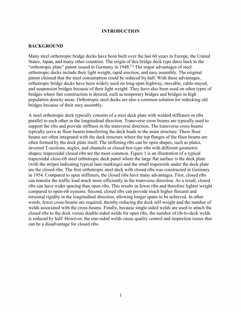
A steel orthotropic deck typically consists of a steel deck plate with welded stiffeners or ribs parallel to each other in the longitudinal direction. Transverse cross beams are typically used to support the ribs and provide stiffness in the transverse direction. The transverse cross beams typically serve as floor beams transferring the deck loads to the main structure. These floor beams are often integrated with the deck structure where the top flanges of the floor beams are often formed by the deck plate itself. The stiffening ribs can be open shapes, such as plates, inverted T-sections, angles, and channels or closed box-type ribs with different geometric shapes; trapezoidal closed ribs are the most common. Figure 1 is an illustration of a typical trapezoidal close-rib steel orthotropic deck panel where the large flat surface is the deck plate (with the stripes indicating typical lane markings) and the small trapezoids under the deck plate are the closed ribs. The first orthotropic steel deck with closed ribs was constructed in Germany in 1954. Compared to open stiffeners, the closed ribs have many advantages. First, closed ribs can transfer the traffic load much more efficiently in the transverse direction. As a result, closed ribs can have wider spacing than open ribs. This results in fewer ribs and therefore lighter weight compared to open-rib systems. Second, closed ribs can provide much higher flexural and torsional rigidity in the longitudinal direction, allowing longer spans to be achieved. In other words, fewer cross-beams are required, thereby reducing the deck self-weight and the number of welds associated with the cross-beams. Finally, because single-sided welds are used to attach the closed ribs to the deck versus double-sided welds for open ribs, the number of rib-to-deck welds is reduced by half. However, the one-sided welds cause quality control and inspection issues that can be a disadvantage for closed ribs.

2

Figure 1. Illustration. Typical closed-rib steel orthotropic deck panel.

To overcome the disadvantages of one-sided welding and prevent premature fatigue failure, more careful consideration is needed to design rib-to-deck welds. Many of the earlier vintage orthotropic decks with closed ribs experienced fatigue cracking problems. There was a lack of knowledge about fatigue and a lack of guidance in the structural design codes. The complex stress state present at the rib-to-deck welds makes fatigue design even more difficult. Many orthotropic decks before the late 1970s were constructed under this state of knowledge. The quest for lighter self-weight led to relatively thin deck plates in the structural design. However, many of the designs with thinner deck plates were vulnerable to high local stress effects from wheel loads. The contribution of the wheel-load effect was not fully considered in early deck designs, and many bridges experienced fatigue cracking problems. Compared to main structural members, orthotropic steel decks tend to have a higher incidence of fatigue problems because of the local effects of wheel loads. Wheel loads cause large local stress variations, stress reversals, and an increased number of stress cycles that must be considered in fatigue design.

Steel orthotropic decks have been part of engineering practice and extensively studied in Europe for decades. Partially to the result of the use of relatively thin deck plates, premature fatigue cracking was observed in many European countries. (See references 2 through 6.) Steel orthotropic decks have also been widely constructed in the United States with mixed experiences relating to fatigue behavior. The situation has been steadily improving as more knowledge becomes available on how to improve fatigue resistance.

OBJECTIVES

The first objective of this study was to determine the effect of weld process and geometry on the fatigue resistance of the rib-deck weld. This was accomplished by fatigue testing a series of 159 specimens with different welding processes and different levels of weld penetration under two different loading regimes. A statistical analysis of the data was used to determine the effect each variable has on fatigue resistance.

The second objective of this research was to optimize the size and shape of rib-to-deck welds as the basis of the detailing requirements. At the time the project began (2008), the fourth edition of the American Association of State Highway and Transportation Officials (AASHTO) Load-and-Resistance Factor Design (LRFD) Bridge Design Specification was the current version.(7) Article 9.8.3.7.2 stated that “Eighty percent partial penetration welds between the webs of a

3

closed rib and the deck plate should be permitted,” and the commentary states that “Such welds, which require careful choice of automatic welding processes and a tight fit, are less susceptible to fatigue failure than full penetration groove welds requiring backup bars.”(7)(pp. 9–23) This provision was commonly perceived as rib-to-deck welds requiring a minimum penetration of 80 percent with a tight fit not to exceed 0.01 inch. An upper bound on penetration is typically applied such that the welds cannot have blow-through or melt-through that creates defects inside the ribs. In reality, because of the thin rib plate thickness that is commonly used in steel orthotropic decks, 80 percent penetration without melt-through or blow-through is difficult to achieve consistently, and, because of to the natural waviness of hot-rolled plate, the tight fit-up was also difficult to consistently achieve. A more tolerant penetration requirement is needed to reduce the need for weld repairs and increase fabrication efficiency. However, any relaxation of the 80 percent penetration must not increase the potential for fatigue cracking.

The last objective of this research was to validate the level 3 design approach currently published in the seventh edition of the AASHTO LRFD Bridge Design Specification (here forth referred to as AASHTO BDS in the remainder of this document) for the design of rib-to-deck welds.(8) This approach adopts a local structural stress (LSS) methodology for fatigue design where three-dimensional finite element models are used to characterize the stress state near weld toes. Stress is interrogated at two points away from the weld toe and then extrapolated to a theoretical stress at the weld toe that is used in the fatigue assessment. Fatigue life data collected in this project will be compared to the extrapolated LSSs based on finite element analysis of the specimens.

APPROACH

Fatigue resistance is typically characterized into S-N curves where fatigue test data is plotted based on the stress range (S) and the number of cycles to failure (N) on a logarithmic scale. Most previous orthotropic deck research used full-scale components to conduct fatigue testing. While this provides an accurate representation of a real structure in terms of boundary conditions and stress fields, the cost of specimens and testing equipment is prohibitively expensive. This research took a different approach where full scale was maintained but through a small test specimen. In this case, a full-thickness deck plate and full-scale rib are welded together into a panel that varied between 3 and 6 ft in length. This creates a full-scale geometry, and the residual welding stresses should be commensurate with a real structure. However, instead of testing the panel to only acquire one fatigue data point, the panel was sectioned into 4-inch-wide specimens, and loads were applied to the rib while supporting the deck, which caused out-of-plane (from the viewpoint of an entire deck) flexing of the rib, placing the weld in a high demand. While this loading pattern does not create a realistic stress pattern in the specimen as compared to a real deck, the concept does allow for rapid and cheap comparison of many specimens testing a variety of different variables on an equal playing ground.

It can be argued that sectioning of the panel reduces the residual stress and that the weak-link concept is lost. The weak-link concept can be illustrated when placing an entire panel under a fatigue test. Likely, that panel will develop a single fatigue crack at some localized point where there is an internal discontinuity within the weld. However, if that panel were sectioned into many smaller specimens, then that localized discontinuity is only within one of them, and that specimen will likely have the lowest fatigue resistance. The argument is that the distribution of

4

fatigue life attained from many specimens extracted from one panel may be different than the distribution produced from testing many single panels. The researchers believe that it was more important to generate a large population of data rather than a small population.

5

EXPERIMENTAL STUDY

SPECIMEN FABRICATION

Either 3- or 6-ft-long weldments were fabricated from a single rib and flat plate meant to represent the deck plate. Two fabricators were used to make the specimens. Most specimens were made by a prominent steel bridge fabricator using typical weld processes. Specimens welded with hybrid laser arc welding (HLAW) were made by a small business that specializes in HLAW. HLAW was integrated into the test program because it produces a higher-quality weld that may lead to higher fatigue resistance.

After welding, the panel was transversely sectioned with a bandsaw to isolate individual 4.25-inch-wide test specimens. The saw-cut edges of the specimens were milled to provide uniform specimen width of 4 inches. Also, a hole was drilled through the flat bottom of the rib plate to enable mounting in the loading frame. The tack weld locations were marked on each specimen to determine whether tack welds influenced the fatigue crack initiation location.

Schematics of each panel sectioning and specimen naming conventions can be found in appendix A.

Welded panels were procured in four distinct batches throughout the life of the project. A byproduct of this was the rib geometry changed slightly from one batch to another. Because this affects the loading of the specimen, figure 2 through figure 4 show the variation in the specimen geometries referred to as types 1–3 rib geometries. Type 1 specimens used a 3/4-inch-thick deck plate and a 5/16-inch-thick rib that was nominally 14 inches tall. Type 2 specimens used a 3/4-inch-thick deck plate and a 5/16-inch-thick rib that was nominally 12 inches tall. Type 3 specimens used a 5/8-inch-thick deck plate and a 5/16-inch-thick rib that was nominally 12 inches tall.

6

Units = Inches.

Figure 2. Illustration. Type 1 rib geometry.

7

Units = Inches.


8

Units = Inches.


The specimen geometries shown in figure 2 through figure 4 represent the as-designed rib, though it was noted during the project that the as-built geometry did deviate from the ideal geometry, but the deviation was not quantified in the project. For instance, the top of the rib was not always parallel to the deck plate, the rib legs were not always perfectly symmetrical, and the height of the rib varied.

TEST MATRIX

Table 1 highlights the major variables explored in the program: welding process, weld penetration, edge preparation, and fit-up gap.

9

Table 1. Test specimen series.

Series Name

Rib Geometry

Welding Process

Target Penetration

(percent)

Rib Plate Beveling

Intentional Fit-up Gap

(inches)

Number of

Specimens

GM8 Type 1 GMAW 80 None 0 16 SA8 Type 1 SAW 80 None 0 16 SA6 Type 1 SAW 60 None 0 8 SA4 Type 1 SAW 40 None 0 8 SA2 Type 1 SAW 20 None 0 8 FIL Type 1 SAW None None 0 8 LP1 Type 1 HLAW 100 Beveled 0 14 LP2 Type 1 HLAW 100 Beveled 0 13 LP3 Type 1 HLAW 100 Beveled 0 14

OB Type 2 SAW None Beveled

(5 degrees over)

0 16

UB Type 2 SAW None Beveled

(5 degrees under)

0 16

OG1 Type 3 SAW 60–100 None 0.02 16 OG2 Type 3 SAW 60–100 None 1/32 16 W Type 3 SAW 60–100 Beveled 0.02 16

GMAW = Gas metal arc welding. SAW = Submerged arc welding.

Three welding processes were explored: GMAW, SAW, and HLAW. It was suggested that weld quality may be a factor between the three processes and may lead to different fatigue lives.

Weld penetration is an obvious variable that may control fatigue life because this is a partial penetration weld under a tensile load. Because partial penetration welds inherently leave an unfused section of the rib at the root, it creates a notch-like defect that could spawn weld root failures. As the penetration value increased, it was thought the fatigue resistance would commensurate.

Edge preparation and fit-up gap are interrelated to the weld penetration, and figure 5 illustrates the differences. Because the rib is trapezoidal, the rib walls intersect the deck plate at a non-normal angle; therefore, without edge preparation, only a corner of the rib wall touches the deck plate prior to welding. This creates a larger face gap than root gap when there is no edge preparation. This requires more weld consumable to fill the larger gap; however, no edge preparation results in larger penetration because there is less base metal to melt in the rib wall, and the wire is able to get closer to the root. When the edge is prepared by milling, it is able to sit flat on the deck plate prior to welding, resulting in less penetration because more rib wall base

10

metal has to be melted. From a fabrication standpoint, edge preparation is not desirable because of the added expense/time in handling the plate and conducting the milling operation. The fit-up gap is related to just the root gap. Because of the natural waviness of hot-rolled plates, a root gap is inevitable, but a tolerance should be provided, and this is referred to as the “fit-up gap.” Larger fit-up gaps can lead to melt-through and blow-through during welding, and small fit-up gaps can increase the cost of fabrication.

Figure 5. Illustration. Comparison of rib edge preparation: beveled (left) and no

preparation (right).

Table 1 also shows horizontal division lines depicting the four distinct batches in which specimens were procured and tested. The first batch of panels was the GM8, SA8, SA6, SA4, SA2, FIL, and LP series. The variable that was targeted was the penetration of the weld and whether it was process dependent. The number in the series title correlates to the target percent penetration (in 10s of percent), GM means that it was made with GMAW, and SA means that it was made with SAW. The FIL series was made with SAW, but the intent was that it would literally be a fillet weld with very little penetration. Because of the face gap from no edge penetration on the rib, the GMAW and SAW processes were unable to attain penetration values less than approximately 60 percent despite attempts to make it vary from 0 to 80 percent. The LP series were made with HLAW, which is inherently intolerant of gaps and by its very nature required edge preparation. The HLAW process was able to consistently achieve 100 percent penetration. Because the two conventional weld processes achieved a consistent penetration, welding process was not considered a variable, and fit-up gap and edge preparation were considered a larger player in achieving the desired weld penetration.

The OB and UB series panels were designed to investigate the influence of the weld root gap and whether weld root failures could be forced to happen. This was done by using an intentionally 5-degree overbeveled and underbeveled edge preparation, as shown in figure 6. The OB

11

specimens were prepared with a bevel angle greater than the rib angle, resulting in a root gap that was open before welding. The UB series had a bevel angle less than the rib angle, resulting in a closed root gap before welding. Despite this bevel preparation, weld shrinkage due to cooling of the weld metal caused the root gaps to close after welding in both series. However, the different bevel preparation resulted in different amounts of contact pressure at the root. The UB series showed definite plastic distortion where the two plates were pressed together from weld shrinkage. This was less evident in the OB series, where the root gap had to close before pressure could develop. Because the OB series did not result in the desired open root gap, they were all saw-cut at the root to open the gap before testing. The saw cuts were performed carefully to avoid contact with the weld, thereby preserving the natural situation at the tip of the root notch. Additionally, half of the UB series had their roots saw-cut. Figure 7 shows typical saw cuts on both the OB and UB specimens.

Figure 6. Illustration. Overbeveled (left) and underbeveled (right) edge preparation.

Figure 7. Photo. Typical saw cuts introduced at the weld roots on the OB and UB

series specimens.

The OG series was meant to explore the effect of potential fit-up gaps that naturally occur as a result of the waviness of hot-rolled plates. No bevel preparation was used. The fabricator used jacks to either lift the rib up or push it down before tacking the rib in place prior to welding. The gap was set using feeler gauges and was mostly uniform along the length of the panel prior to welding. The OG1 panel had an intentional 0.020-inch gap placed where the OG2 panel had an intentional 0.031-inch gap. This is illustrated in figure 8.

12

Units = Inches.

Figure 8. Illustration. Intentional fit-up gaps in OG1 panel (left) and OG2 panel (right).

The last panel fabricated was the W series and was meant to include all the lessons learned from the previous sets of panels to attain a target penetration of 70 percent with variance allowed between 60 and 100 percent. The edge was bevel prepared by the fabricator to attain better control over the penetration. In addition, a 0.020-inch fit-up gap was purposely introduced. This is illustrated in figure 9.

13

Units = Inches.

Figure 9. Illustration. Fit-up gap and edge preparation for W series.

Residual stress is a key factor in the fatigue performance of welded joints; therefore, tests were performed at different load ratios (R-ratios) to study their effect on fatigue life, though this is not reflected in table 1. The R-ratio represents the ratio between the minimum and maximum loads of the applied load cycle. The stress cycle is under full tension when R = 0, and it is under an equal tension-compression stress reversal when R = −1. Only ratios of 0 and −1 were explored in this program. Comparison of fatigue results from the two test conditions can help determine how much of the compression stress range is being placed in relative tension as a result of superposition of residual stresses. The R = 0 test condition will provide a lower bound for fatigue life. Each test series had a blend of specimens tested at both load ratios.

14

TEST SETUP AND PROCEDURE

Fatigue tests were conducted concurrently at both the Structures Laboratory at the Turner-Fairbank Highway Research Center (TFHRC) and the Structures Laboratory at Virginia Tech (VT). Each testing site both used closed-loop, servo valve-controlled hydraulic testing frames. The following subsections describe the loading fixture and testing procedures.

Test Setup

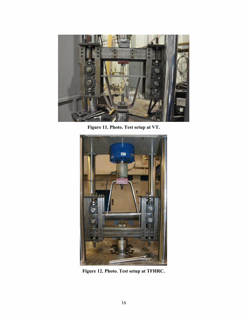
Two customized test fixtures were fabricated to hold a specimen and facilitate applying loads in the universal testing machines. An illustration of the customized fixture is shown in figure 10. Conceptually, the fixture was a spreader beam that supported four adjustable rollers. The rollers were meant to clamp the deck plate so it could resist full load reversals. Each of the rollers was supported by two take-up bearings. The bearings could allow some angular adjustment so the rollers could be adjusted to be parallel to the deck plate surface. The welded test specimens had a certain amount of plate distortion induced by welding. The angular adjustment capability of the rollers was essential to allow the rollers to adapt to the specimen and prevent distortional twisting that could cause error in the applied stress range. This fixture was mounted to either the actuator piston or load cell, depending on the preference of each test site.

15

Units = Inches.

Figure 10. Illustration. Test setup.

The flat of the rib attached to the other side of the machine from the customized fixture. To uniformly load across the width of the rib, the rib was sandwiched between two thick plate washers. The thick plate washers were 5 inches long at TFHRC but only 3.75 inches long at VT. This is specifically noted because it slightly altered the loading in the specimens between the two testing sites. In addition, since the rib flat was typically not parallel to the deck plate, spherical washers were placed between the thick plate washer and the testing machine to ensure the deck plate sat parallel to the hollow structural section of the customized fixture.

Photos of the fixture and a specimen mounted into the testing frames at each of the test sites are shown in figure 11 and figure 12.

16

Figure 11. Photo. Test setup at VT.

Figure 12. Photo. Test setup at TFHRC.

17

Test Procedure

Consistent boundary conditions between specimens were essential to minimize scatter in the test results. Ideally, the top and bottom rollers should have provided ideal boundary conditions. However, excessive clamping force between the two rollers could potentially add some fixity. The stress state at the potential cracking locations was expected to change dramatically if fixed-end conditions existed instead of the ideal rollers. Too much clamping force from the rollers on the deck plate could cause roller friction that would effectively create a semi-fixed boundary condition. Too little clamping force would introduce slip in the load path and allow the specimen to bang and vibrate in the test fixture under load reversal. Therefore, an installation procedure was initiated to measure and limit the clamping force to ensure that the ideal roller boundary condition was present. After a few trials, the clamping force was set to 70 lb on each side (140 lb in total). The force was measured by monitoring the load cell output during the clamping procedure while in displacement control. Rollers on one side of the deck plate were brought into contact with the deck plate equally until the load cell read 140 lb, and then the rollers on the other side were brought into contact until the load cell registered 0 lb. It was observed that the rollers were still able to rotate freely at this clamping force level.

19

LSS ANALYSIS

The specimens were analyzed according to the level 3 design procedures outlined in AASHTO BDS to attain the LSS range. This design philosophy is based on the International Institute of Welding (IIW) document entitled Recommendations for Fatigue Design of Welded Joints and Components.(9) The LSS is defined via linear extrapolation of surfaces stress near the weld toe to the weld toe location. AASHTO BDS adopted the IIW coarse meshing option where the mesh size at the weld has element dimensions of approximately t by t, where t is the plate thickness. The IIW method requires extrapolating stresses from 0.5t and 1.5t distance away from the weld toe. It is further suggested that stresses are taken at mid-side nodes, suggesting that quadratic element formulations are used. This also requires two rows of elements, each t long, meshed on the extrapolated side of the weld toe. This is better shown in figure 13 where the geometry of the mid-plate thickness is shown. At the line defining the weld toe, two parallel lines are offset up the rib (generally in the Y direction) and across the deck plate (in the X direction). These parallel lines are offset by the thickness of the respective plates. Only one element width would be meshed between these parallel lines, and the mesh would be seeded across the width of the specimen (in the Z direction) such that the element width would be approximately t.

20

Units = Inches.

Figure 13. Illustration. Partitioning of specimen.

Since each lab used a different-sized thick plate washer to clamp the rib to the testing machine, each model was analyzed considering these two boundary conditions. Figure 13 shows a hatched area at the top of the rib. This hatched area was either 3.75 or 5 inches in the X direction for the specimens tested at VT and TFHRC, respectively. This area of the rib was modeled with a shell thickness of 2 inches to represent the added stiffness provided by the two thick plate washers. A unit point load was applied at the center of the hatched area to represent the applied load to the specimen. Because the specimens remained elastic, the results from this unit load analysis were multiplied by the applied load range to attain LSS ranges.

Finite element models were constructed with an analysis program capable of capturing nonlinear material and nonlinear geometric behavior; however, the models were fully elastic following the level 3 design procedure. A typical mesh is shown in figure 14. The mesh may appear discontinuous at the intersection of the rib and deck. With the restriction of approximately t by t element dimensions, it becomes difficult to attain a continuous mesh when there are large

21

disparities in the plate thicknesses, such as this case, where the deck plate is over twice as thick as the rib plate. However, the analysis program has the capability of enforcing surface-based tie constraints between different parts. In this case, the rib and deck are modeled as individual parts and then assembled together with tie constraints to represent the weld. Tie constraints have no volume or mass; they merely enforce compatibility between two meshes. This enforces compatible displacements and rotations between the incompatible meshes through interpolation between node regions. Therefore, the rib and deck plates could be modeled with their respective t by t element dimensions within the same model.

Figure 14. Illustration. Meshed specimen.

As mentioned previously, only a unit load was modeled at the middle of the rib top. The resulting stress contours through a typical specimen is shown in figure 15 superimposed on the deflected shape. This contour plot shows the stresses at the element surfaces near the weld toe; these are in a direction perpendicular to the weld toe. The local structural extrapolation required interrogation of mid-side nodes at a distance of 0.5 and 1.5 plate thicknesses from the intersection. In AASHTO BDS, these are called the f0.5 and f1.5 stresess, and they should be in the direction perpendicular to the weld toe. The illustration shown in figure 16 is a zoomed-in view of figure 15 to just the weld region. Also shown by black dots are the mid-side nodes where the f0.5 and f1.5 stresses are taken for both the rib and deck plate. The model ignored the geometry of the weld as a simplification, and, because of this, the extrapolation was to the plate intersection, not the location of the theoretical weld toe. This was done for two reasons: (1) it was thought this would be a conservative assumption, and (2) all of the welds tested had quite a variation in weld geometry, so it would have been burdensome to model every specimen in lieu of just ignoring the weld.

22

Figure 15. Illustration. Membrane stress in specimen under unit load.

23

Figure 16. Illustration. Extrapolation points from rib and deck plate.

LSS results from all the models are shown in table 2 through table 4, respectively, for the types 1–3 specimen geometries. Because the models were based on unit loads, the f0.5 and f1.5 stresses reported are from the unit load. The flss stress is the actual LSS based on extrapolation. Because of the unit load analysis, all stresses are reported in units of ksi per kip of load. This was purposeful because in the fatigue analysis of the specimens, the flss value only had to be multiplied by the load range applied to the specimen to attain the total LSS range.

Table 2. LSSs from unit load for type 1 geometry.

Test Lab Location f0.5 (ksi)

f1.5 (ksi)

flss (ksi)

TFHRC Deck plate 6.662 5.327 7.330 Rib wall 7.053 6.522 7.318

Weld root 4.710 4.319 4.906

VT Deck plate 6.663 5.328 7.331 Rib wall 7.682 7.085 7.981

24


Location f0.5 (ksi)

f1.5 (ksi)

flss (ksi)

Deck plate 6.663 5.331 7.329 Rib wall 8.246 7.581 8.579 Weld root 5.906 5.378 6.170


Test Lab Location f0.5 (ksi)

f1.5 (ksi)

flss (ksi)

TFHRC Deck plate 9.734 7.692 10.755 Rib wall 11.035 10.174 11.466

VT Deck plate 9.733 7.692 10.754 Rib wall 11.457 10.547 11.912

Because of the boundary condition differences between the two labs, table 2 and table 4 report different flss values for each lab, as those rib geometries were tested at each lab. The type 2 geometry in table 3 was only tested at VT.

Finally, it can be noted that in table 2 and table 3, LSSs are also reported at the weld root. The LSS method was never intended for characterizing the stress state at a weld root. However, in this research, some specimens failed from the weld root, and, to plot those failures relative to all the other data, the LSS was extrapolated on the inside surface of the rib wall to represent the LSS of the weld root.

25

RESULTS

The raw data for all of the fatigue results are shown in table 5 through table 17 for all of the different series of panels tested. Each table reports the minimum and maximum loads applied to the specimen, the total force range, the load ratio, the percent penetration that was achieved (calculated as the projection of rib thickness onto the deck plate by the penetration measured along the deck plate), failure mode (either in the deck plate, rib wall, or weld root), LSS, and the number of cycles to failure. Finally, the tables report the root condition that existed in the as-welded condition.

26

Table 5. GM8 series results.

Specimen ID Minimum/ Maximum

Loads (kips)

Load Ratio

Load Range (kips)

Root Gap Penetration (percent) Failure Mode

LSS Range (ksi)

Cycles to Failure

GM8-1 2.75/−2.75 −1 5.50 Close 72.7 Deck weld toe 40.32 888,807 GM8-2 0.00/5.00 0 5.00 Close 73.3 Runout 36.65 20,000,655 GM8-3 0.00/2.75 0 2.75 Close 79.0 Deck weld toe 20.16 18,253,515 GM8-4 2.50/−2.50 −1 5.00 Close 67.0 Weld root 24.53a 6,060,816 GM8-5 2.75/−2.75 −1 5.50 Close 81.2 Deck weld toe 40.32 770,672 GM8-6 2.50/−2.50 −1 5.00 Close 79.1 Deck weld toe 36.65 1,517,705 GM8-7 2.75/−2.75 −1 5.50 Close 83.0 Deck weld toe 40.32 751,609 GM8-8 0.00/5.00 0 5.00 Close 69.3 Deck weld toe 36.65 302,451 GM8-9 1.25/−1.25 −1 2.50 Close 84.1 Runout 18.33 10,000,000 GM8-10 0.00/5.00 0 5.00 Close 85.3 Deck weld toe 36.65 296,571 GM8-11 2.50/−2.50 −1 5.00 Close 88.8 Deck weld toe 36.65 1,390,062 GM8-12 2.00/−2.00 −1 4.00 Close 87.8 Deck weld toe 29.32 2,112,094 GM8-13 1.25/−1.25 −1 2.50 Close 94.5 Runout 18.33 10,000,000 GM8-14 0.00/6.00 0 6.00 Close 77.9 Deck weld toe 43.98 146,635 GM8-15 2.50/−2.50 −1 5.00 Close 96.5 Deck weld toe 36.65 863,459 GM8-16 2.50/−2.50 −1 5.00 Close 83.3 Deck weld toe 36.65 1,657,918

aLSS analysis is only applicable to the analysis of weld toe cracking. LSS range reported is based on extrapolation of stresses on the inside surface of the rib. ID = Identification.

27

Table 6. SA8 series results.


Loads (kips)

Load Ratio

Load Range (kips)


LSS Range (ksi)

Cycles to Failure

SA8-1 2.50/−2.50 −1 5.00 Close 58.5 Rib weld toe 39.91 689,134 SA8-3 2.50/−2.50 −1 5.00 Close 53.0 Rib weld toe 39.91 3,732,998 SA8-4 2.50/−2.50 −1 5.00 Close 76.2 Rib weld toe 39.91 2,321,046 SA8-5 2.50/−2.50 −1 5.00 Close 73.8 Deck weld toe 36.66 3,332,973 SA8-6 2.50/−2.50 −1 5.00 Close 66.5 Deck weld toe 36.66 2,623,398 SA8-7 2.50/−2.50 −1 5.00 Close 67.9 Rib weld toe 39.91 3,399,577 SA8-8 2.50/−2.50 −1 5.00 Close 56.0 Rib weld toe 39.91 2,743,534 SA8-9 2.75/−2.75 −1 5.50 Close 53.4 Rib weld toe 43.90 283,556 SA8-10 2.50/−2.50 −1 5.00 Close 51.9 Rib weld toe 39.91 869,732 SA8-11 2.75/−2.75 −1 5.50 Close 60.4 Rib weld toe 43.90 617,702 SA8-12 2.75/−2.75 −1 5.50 Close 73.1 Deck weld toe 40.32 1,930,296 SA8-13 2.75/−2.75 −1 5.50 Close 72.7 Deck weld toe 40.32 1,782,037 SA8-14 0.00/5.00 0 5.00 Close 71.6 Deck weld toe 36.66 1,417,734 SA8-15 0.00/5.00 0 5.00 Close 67.1 Deck weld toe 36.66 943,434 SA8-16 0.00/5.00 0 5.00 Close 74.4 Deck weld toe 36.66 927,241

28



Loads (kips)

Load Ratio

Load Range (kips)


LSS Range (ksi)

Cycles to Failure

SA6-1 0.00/5.00 0 5.00 Close 72.8 Deck weld toe 36.65 317,140 SA6-2 0.00/5.00 0 5.00 Close 70.0 Deck weld toe 36.65 257,016 SA6-3 0.00/5.00 0 5.00 Close 66.2 Deck weld toe 36.65 286,626 SA6-4 2.75/−2.75 −1 5.50 Close 71.3 Deck weld toe 40.32 629,917 SA6-5 2.75/−2.75 −1 5.50 Close 65.4 Deck weld toe 40.32 2,074,221 SA6-6 2.75/−2.75 −1 5.50 Close 72.3 Deck weld toe 40.32 860,759 SA6-7 2.75/−2.75 −1 5.50 Close 69.3 Deck weld toe 40.32 588,156 SA6-8 2.75/−2.75 −1 5.50 Close 64.7 Deck weld toe 40.32 521,486



Loads (kips)

Load Ratio

Load Range (kips)


LSS Range (ksi)

Cycles to Failure

SA4-1 2.75/−2.75 −1 5.50 Close 58.3 Deck weld toe 40.32 643,413 SA4-2 2.75/−2.75 −1 5.50 Closea 62.6 Deck weld toe 40.32 540,472 SA4-3 2.75/−2.75 −1 5.50 Close 57.0 Deck weld toe 40.32 607,547 SA4-4 2.75/−2.75 −1 5.50 Close 59.5 Deck weld toe 40.32 840,760 SA4-5 2.75/−2.75 −1 5.50 Close 61.8 Deck weld toe 40.32 649,093 SA4-6 0.00/5.00 0 5.00 Close 58.2 Deck weld toe 36.65 294,621 SA4-7 0.00/5.00 0 5.00 Close 52.3 Deck weld toe 36.65 300,716 SA4-8 0.00/5.00 0 5.00 Close 66.1 Deck weld toe 36.65 407,819

aSide opposite the failure did have an open gap.

29



Loads (kips)

Load Ratio

Load Range (kips)


LSS Range (ksi)

Cycles to Failure

SA2-1 2.75/−2.75 −1 5.50 Close 89.1 Deck weld toe 40.32 750,996 SA2-2 2.75/−2.75 −1 5.50 Close 66.8 Deck weld toe 40.32 2,690,351 SA2-3 2.75/−2.75 −1 5.50 Close 71.4 Deck weld toe 40.32 708,693 SA2-4 2.75/−2.75 −1 5.50 Close 65.2 Deck weld toe 40.32 381,990 SA2-5 2.75/−2.75 −1 5.50 Close 62.0 Deck weld toe 40.32 534,364 SA2-6 0.00/5.00 0 5.00 Close 64.1 Deck weld toe 36.65 258,639 SA2-7 0.00/5.00 0 5.00 Close 71.4 Deck weld toe 36.65 222,741 SA2-8 0.00/5.00 0 5.00 Close 64.5 Deck weld toe 36.65 238,136

Table 10. FIL series results.


Loads (kips)

Load Ratio

Load Range (kips)


LSS Range (ksi)

Cycles to Failure

FIL-1 0.00/5.00 0 5.00 Close 66.1 Deck weld toe 36.65 308,351 FIL-2 0.00/5.00 0 5.00 Close 58.5 Deck weld toe 36.65 352,981 FIL-3 0.00/5.00 0 5.00 Close 64.2 Deck weld toe 36.65 302,927 FIL-4 2.75/−2.75 −1 5.50 Close 67.2 Deck weld toe 40.32 698,763 FIL-5 2.75/−2.75 −1 5.50 Close 62.8 Deck weld toe 40.32 855,918 FIL-6 2.75/−2.75 −1 5.50 Close 65.1 Deck weld toe 40.32 2,179,319 FIL-7 2.75/−2.75 −1 5.50 Close 46.4 Deck weld toe 40.32 870,418 FIL-8 2.75/−2.75 −1 5.50 Close 69.6 Deck weld toe 40.32 529,113

30

Table 11. LP1 and LP2 series results.


Loads (kips)

Load Ratio

Load Range (kips)


LSS Range (ksi)

Cycles to Failure

LP1-1 0.00/5.00 0 5.00 None 100 Deck weld toe 36.65 278,209 LP1-2 0.00/5.00 0 5.00 None 100 Deck weld toe 36.65 193,114 LP1-3 2.75/−2.75 −1 5.50 None 100 Deck weld toe 40.32 302,479 LP1-4 2.75/−2.75 −1 5.50 None 100 Deck weld toe 40.32 235,185 LP1-5 2.75/−2.75 −1 5.50 None 100 Deck weld toe 40.32 315,624 LP1-6 2.75/−2.75 −1 5.50 None 100 Deck weld toe 40.32 367,003 LP1-7 2.75/−2.75 −1 5.50 None 100 Deck weld toe 40.32 367,875 LP1-8 2.75/−2.75 −1 5.50 None 100 Deck weld toe 40.32 407,218 LP1-9 3.00/−3.00 −1 6.00 None 100 Deck weld toe 43.98 381,539 LP1-10 2.75/−2.75 −1 5.50 None 100 Deck weld toe 40.32 513,805 LP1-12 2.75/−2.75 −1 5.50 None 100 Deck weld toe 40.32 552,488 LP1-13 2.75/−2.75 −1 5.50 None 100 Deck weld toe 40.32 492,048 LP1-14 2.75/−2.75 −1 5.50 None 100 Deck weld toe 40.32 435,953 LP1-15 2.75/−2.75 −1 5.50 None 100 Deck weld toe 40.32 404,372 LP2-1 1.60/−1.60 −1 3.20 None 100 Deck weld toe 23.46 1,788,904 LP2-2 1.60/−1.60 −1 3.20 None 100 Deck weld toe 23.46 2,956,726 LP2-3 1.60/−1.60 −1 3.20 None 100 Deck weld toe 23.46 2,898,356 LP2-4 1.60/−1.60 −1 3.20 None 100 Deck weld toe 23.46 2,448,412 LP2-5 1.60/−1.60 −1 3.20 None 100 Deck weld toe 23.46 3,276,984 LP2-6 1.60/−1.60 −1 3.20 None 100 Deck weld toe 23.46 2,440,312 LP2-7 1.60/−1.60 −1 3.20 None 100 b 23.46 635,000 LP2-8 0.00/3.20 0 3.20 None 100 Deck weld toe 23.46 2,021,012

31


Loads (kips)

Load Ratio

Load Range (kips)


LSS Range (ksi)

Cycles to Failure

LP2-9 0.00/3.20 0 3.20 None 100 Deck weld toe 23.46 741,520 LP2-10 0.00/3.20 0 3.20 None 100 Deck weld toe 23.46 967,256 LP2-11 0.00/3.20 0 3.20 None 100 Deck weld toe 23.46 1,138,650 LP2-12 0.00/3.20 0 3.20 None 100 Deck weld toe 23.46 861,537 LP2-13 0.00/3.20 0 3.20 None 100 Deck weld toe 23.46 992,876 LP2-14a 0.00/3.20 0 3.20 None Not measured Deck weld toe 23.46 1,320,314

aThis specimen was not HLAW welded; it was just fillet welds used to hold the rib in place for HLAW. bData quality was questionable due to lack of documentation for this particular specimen, and, based on unusually low fatigue resistance, it was not included in any analysis.

32

Table 12. LP3 series results.


Loads (kips)

Load Ratio

Load Range (kips)


LSS Range (ksi)

Cycles to Failure

LP3-0a 2.75/−2.75 −1 5.50 None Not measured Deck weld toe 40.32 1,262,905 LP3-1 2.75/−2.75 −1 5.50 None 100 Deck weld toe 40.32 471,293 LP3-2 0.00/5.00 0 5.00 None 100 Deck weld toe 36.65 208,968 LP3-3 2.75/−2.75 −1 5.50 None 100 Deck weld toe 40.32 251,375 LP3-4 2.75/−2.75 −1 5.50 None 100 Deck weld toe 40.32 338,584 LP3-5 0.00/5.00 0 5.00 None 100 Deck weld toe 36.65 169,658 LP3-6 2.75/−2.75 −1 5.50 None 100 Deck weld toe 40.32 474,830 LP3-7 0.00/4.00 0 4.00 None 100 Deck weld toe 29.32 302,748 LP3-8 0.00/4.00 0 4.00 None 100 Deck weld toe 29.32 425,770 LP3-9 0.00/4.00 0 4.00 None 100 Deck weld toe 29.32 361,781 LP3-10 0.00/4.00 0 4.00 None 100 Deck weld toe 29.32 502,781 LP3-11 0.00/4.00 0 4.00 None 100 Deck weld toe 29.32 477,681 LP3-12 0.00/4.00 0 4.00 None 100 Deck weld toe 29.32 430,735 LP3-13a 0.00/3.20 0 3.20 None Not measured Deck weld toe 23.46 5,407,198

aThis specimen was not HLAW welded; it used fillet welds to hold the rib in place for HLAW.

33

Table 13. OB series results.


Loads (kips)

Load Ratio

Load Range (kips)


LSS Range (ksi)

Cycles to Failure

OB-1 2.50/−2.50 −1 5.00 Open 45.2 Weld root 30.85a 647,879 OB-2 2.50/−2.50 −1 5.00 Open 65.1 Weld root 30.85a 981,142 OB-3 2.50/−2.50 −1 5.00 Open 67.0 Weld root 30.85a 2,385,939 OB-4 2.50/−2.50 −1 5.00 Open 80.6 Weld root 30.85a 1,376,487 OB-5 0.00/5.00 0 5.00 Open 66.5 Deck weld toe 36.65 574,148 OB-6 0.00/5.00 0 5.00 Open 66.3 Deck weld toe 36.65 688,273 OB-7 2.75/−2.75 −1 5.50 Open 66.0 Weld root 33.94a 1,076,871 OB-8 2.75/−2.75 −1 5.50 Open 70.1 Weld root 33.94a 618,383 OB-9 2.50/−2.50 −1 5.00 Open 76.3 Weld root 30.85a 2,451,238 OB-10 2.50/−2.50 −1 5.00 Open 52.8 Weld root 30.85a 1,056,726 OB-11 2.50/−2.50 −1 5.00 Open 54.2 Weld root 30.85a 996,626 OB-12 2.50/−2.50 −1 5.00 Open 65.8 Weld root 30.85a 1,316,952 OB-13 0.00/5.00 0 5.00 Open 67.7 Deck weld toe 36.65 990,806 OB-14 0.00/5.00 0 5.00 Open 57.1 Deck weld toe 36.65 979,089 OB-15 2.75/−2.75 −1 5.50 Open 64.8 Rib weld toe 47.18 660,272 OB-16 2.75/−2.75 −1 5.50 Open 51.6 Weld root 33.94a 768,171

aLSS analysis is only applicable to the analysis of weld toe cracking. LSS range reported is based on extrapolation of stresses on the inside surface of the rib.

34

Table 14. UB series results.


Loads (kips)

Load Ratio

Load Range (kips)


LSS Range (ksi)

Cycles to Failure

UB-1 2.50/−2.50 −1 5.00 Close 65.1 Deck weld toe 36.65 1,359,570 UB-2 2.50/−2.50 −1 5.00 Close 68.8 Weld root 30.85a 694,734 UB-3 2.50/−2.50 −1 5.00 Close 65.1 Rib weld toe 42.90 2,011,029 UB-4 2.50/−2.50 −1 5.00 Close 60.7 Deck weld toe 36.65 1,372,641 UB-5 0.00/5.00 0 5.00 Close 65.6 Deck weld toe 36.65 386,829 UB-6 0.00/5.00 0 5.00 Close 66.2 Deck weld toe 36.65 474,226 UB-7 2.75/−2.75 −1 5.50 Close 72.9 Deck weld toe 40.31 1,292,525 UB-8 2.75/−2.75 −1 5.50 Close 70.7 Deck weld toe 40.31 1,182,601 UB-9 2.50/−2.50 −1 5.00 Open 76.4 Deck weld toe 36.65 2,024,920 UB-10 2.50/−2.50 −1 5.00 Open 69.8 Runout 36.65 4,725,868 UB-11 2.50/−2.50 −1 5.00 Open 54.6 Weld root 30.85a 1,483,203 UB-12 2.50/−2.50 −1 5.00 Open 54.0 Weld root 30.85a 1,590,018 UB-13 0.00/5.00 0 5.00 Open 45.4 Rib weld toe 42.90 448,014 UB-14 0.00/5.00 0 5.00 Open 64.4 Deck weld toe 36.65 591,939 UB-15 2.75/−2.75 −1 5.50 Open 64.9 Weld root 33.94a 856,676 UB-16 2.75/−2.75 −1 5.50 Open 57.4 Rib weld toe 47.18 1,177,345

aLSS analysis is only applicable to the analysis of weld toe cracking. LSS range reported is based on extrapolation of stresses on the inside surface of the rib.

35

Table 15. OG1 series results.


Loads (kips)

Load Ratio

Load Range (kips)

Root Gapa (inches)

Penetration (percent) Failure Mode

LSS Range (ksi)

Cycles to Failure

OG-1 2.75/−2.75 −1 5.50 0.000 b Rib weld toe 65.52 716,527 OG-2 2.75/−2.75 −1 5.50 0.000 b Deck weld toe 59.15 674,990 OG-3 2.75/−2.75 −1 5.50 0.000 b Deck weld toe 59.15 536,828 OG-4 — — — 0.000 — — — — OG-5 — — — 0.000 — — — —

OG-6 — — — 0.013 0.000 — — — —

OG-7 — — — 0.005 0.000 — — — —

OG-8 — — — 0.006 0.000 — — — —

OG-9 — — — 0.006 0.007 — — — —

OG-10 — — — 0.000 — — — — OG-11 — — — 0.000 — — — — OG-12 — — — 0.000 — — — — OG-13 — — — 0.000 — — — —

OG-14 — — — 0.000 0.003 — — — —

OG-15 — — — 0.000 0.009 — — — —

OG-16 — — — 0.000 0.007 — — — —

aThe target pre-weld gap was 0.020 inch. When two numbers are presented in a cell, they represent measurements that were different on each of the rib legs. bMacro-etch was never performed, so weld dimensions could not be reported. —Specimen was accidently destroyed (no data to report).

36

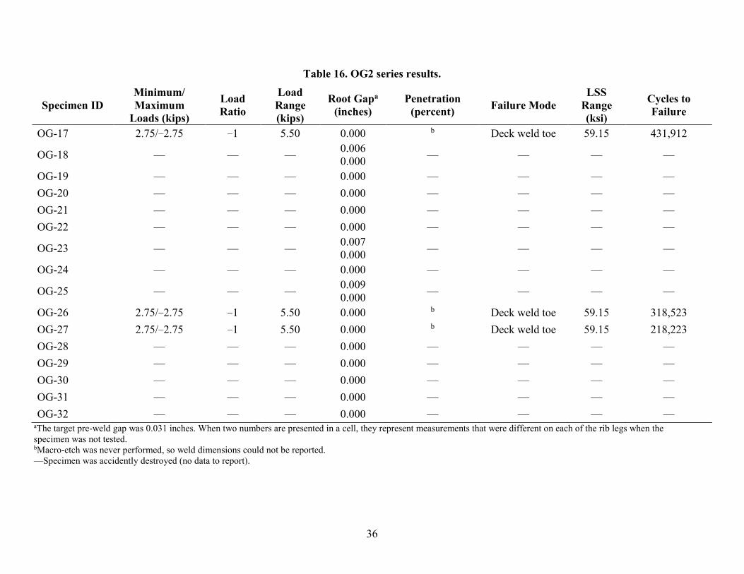
Table 16. OG2 series results.


Loads (kips)

Load Ratio

Load Range (kips)

Root Gapa

(inches) Penetration

(percent) Failure Mode LSS

Range (ksi)

Cycles to Failure

OG-17 2.75/−2.75 −1 5.50 0.000 b Deck weld toe 59.15 431,912

OG-18 — — — 0.006 0.000 — — — —

OG-19 — — — 0.000 — — — — OG-20 — — — 0.000 — — — — OG-21 — — — 0.000 — — — — OG-22 — — — 0.000 — — — —

OG-23 — — — 0.007 0.000 — — — —

OG-24 — — — 0.000 — — — —

OG-25 — — — 0.009 0.000 — — — —

OG-26 2.75/−2.75 −1 5.50 0.000 b Deck weld toe 59.15 318,523 OG-27 2.75/−2.75 −1 5.50 0.000 b Deck weld toe 59.15 218,223 OG-28 — — — 0.000 — — — — OG-29 — — — 0.000 — — — — OG-30 — — — 0.000 — — — — OG-31 — — — 0.000 — — — — OG-32 — — — 0.000 — — — —

aThe target pre-weld gap was 0.031 inches. When two numbers are presented in a cell, they represent measurements that were different on each of the rib legs when the specimen was not tested. bMacro-etch was never performed, so weld dimensions could not be reported. —Specimen was accidently destroyed (no data to report).

37

Table 17. W series results.


Loads (kips)

Load Ratio

Load Range (kips)


LSS Range (ksi)

Cycles to Failure

W-1 1.50/−1.50 −1 3.00 Closed 32.7 Deck weld toe 32.27 2,852,314 W-2 0.00/4.00 0 4.00 Closed 32.4 Deck weld toe 43.02 341,178 W-3 2.00/−2.00 −1 4.00 Closed 40.7 Deck weld toe 43.02 972,348 W-4 0.00/3.00 0 3.00 Closed 42.3 Deck weld toe 32.27 600,935 W-5 2.00/−2.00 −1 4.00 Closed 33.2 Deck weld toe 43.02 859,795 W-6 0.00/3.00 0 3.00 Closed 38.0 Deck weld toe 32.27 689,455 W-7 2.00/−2.00 −1 4.00 Closeda 47.4 Rib weld toe 45.86 795,766 W-8 0.00/3.00 0 3.00 Closeda 45.6 Deck weld toe 32.27 552,962 W-9 2.00/−2.00 −1 4.00 Closed 36.6 Deck weld toe 43.02 858,519 W-10 0.00/3.20 0 3.20 Closed 36.4 Deck weld toe 34.42 483,507 W-11 2.20/−2.20 −1 4.40 Open 34.9 Deck weld toe 47.32 512,260 W-12 0.00/3.20 0 3.20 Closed 40.3 Deck weld toe 34.42 403,150 W-13 2.20/−2.20 −1 4.40 Closed 46.5 Deck weld toe 47.32 655,818 W-14 0.00/3.00 0 3.00 Closed 31.4 Deck weld toe 32.27 624,567 W-15 2.00/−2.00 −1 4.00 Closed 38.5 Deck weld toe 43.02 1,211,796 W-16 0.00/3.00 0 3.00 Closed 40.0 Deck weld toe 32.27 980,335

aSide opposite the failure did have an open gap.

38

ROOT CONDITION

Root condition is controlled by fit-up tolerance between the rib and deck plate prior to welding. The root condition being open or closed was only determined visually. As previously described, the OB and UB series had many specimens with purposeful saw cuts to expose the root, and these were obviously open conditions (as shown in figure 7). The open condition can also occur naturally, as shown in the macro in figure 17, where the inside corner of the rib was not in contact with the deck plate prior to welding, and weld shrinkage did not close that gap. For the specimens that had purposeful fit-up gaps introduced, it was observed in most instances that the gap would disappear from weld shrinkage. This is mainly shown in table 15 through table 17. For the OG1, OG2, and W series specimens covered in these tables, the fabricator tack welded the rib to deck with pre-set gaps along the entire length of the panel before final welding. This was done by clamping and jacking the rib relative to the deck plate using feeler gauges to set the gap. The rib was tacked approximately every 6 inches. The OG1 and W panels had a 0.020-inch pre-weld gap, and the OG2 panel had a 0.031-inch gap.

Figure 17. Photo. Macro of specimen SA4-2 (example of open root condition).

Once the OG1 and OG2 panels had been cut up into distinct specimens, feeler gauges were once again used to see if they could be inserted into the root on each side of the specimen. For the OG1 panel with a pre-weld gap of 0.020 inch, it can be seen in in table 15 that of the 32 roots, a feeler gauge could not be inserted into 25 of them. The remaining seven had measurable gaps varying from 0.003 to 0.013 inch. The OG2 panel had a pre-weld gap of 0.031 inch, and it can be seen in table 16 that of the 32 roots measured after welding, 29 had fully closed, with the remaining 3 with measurable gaps varying from 0.006 to 0.009 inch. Unfortunately, the W series specimen gaps were not measured with feeler gauges; and the determination was made strictly based on visual appearance from the weld macro of each specimen.

The closed root condition was interpreted as a condition where the unfused portion of the rib was in contact or almost in contact with the deck plate. A photo of the closed root condition is shown in figure 18; the inside corner of the rib was plastically deformed into the deck plate from the weld shrinkage. Figure 19 and figure 20 show photos from two W series specimen welds. Because this panel used a rib beveled to sit flush on the deck plate, 29 of the welds from all the specimens looked like the photo in figure 19, and this was considered to be a closed root condition. Three of the weld macros from the W series panel specimens looked like the specimen

39

in figure 20 where there was a gap at the root (likely formed because the bevel was not fully machined), and this was considered to be an open root condition. In the closed root condition, stresses could be transferred through bearing between the rib and deck plates without large deformation to the rib.

Figure 18. Photo. Macro of specimen SA6-1 (example of closed root condition).

Figure 19. Photo. Macro of specimen W-1.

40

Figure 20. Photo. Macro of specimen W-11.

FATIGUE RESULTS

Several additional points should be noted when reviewing table 5 through table 17. First, all of the HLAW-welded panels achieved 100-percent penetration through visual inspection of the cross section exposed at the edge of each specimen. In fact, the weld root even had a small amount of reinforcement, indicating that penetration even exceeded 100 percent at times. However, in the tables, a value of 100 percent was assumed. Taking photos of every HLAW weld was deemed unproductive because the photos were only being used for attaining weld penetration, which was greater than or equal to 100 percent. Therefore, only 10 specimens had their weld cross sections photographed. As the program progressed, the photographs of all specimens were used to define further geometric variables beyond just penetration. However, the data for the HLAW series of panels may appear incomplete for this reason.

Second, most of the specimens from the OG1 and OG2 panel were accidently destroyed before they were tested. In addition, none of the photographs of the weld cross sections were preserved, and this gap appears in the data tables in appendix B.

The data from all specimens tested at a load ratio of −1 are plotted as blue-filled squares in figure 21 in S-N format against the AASHTO category B, C, and D curves. The heavy line represents the lower bound of the data (i.e., mean minus two standard deviations) and plots slightly above the category B curve. The data from all specimens tested at a load ratio of zero are plotted as circles in figure 22. The heavy line represents the lower bound of the data and plots just below the category C curve. The difference between these two results comes down to magnitude of residual stress and how effective the compression portion of the fatigue cycle is for R = −1 loading. Because it is nearly impossible to predict the load ratio in design because residual stresses are not known, it would be best to categorize the rib-to-deck weld based on tension-only loaded specimens.

41

Figure 21. Graph. Plot of all R = −1 data.

Figure 22. Graph. Plot of all R = 0 data.

The data from all weld root failures, which coincidently only occurred at load ratios of −1, are plotted as triangles in figure 23. The heavy green line represents the lower bound of the data and plots slightly above the category B curve. This indicates that according to the LSS procedure implemented in this document, weld root failures would be a category B detail. However, the procedure was slightly unconventional and used the LSSs on the inside of the rib wall that

1

10

100

0.1 1.0 10.0 100.0

LSS

Ran

ge (k

si)

Cycles to Failure (millions)

R= -1

R= -1 (95% confidence)

Runout

Cat B

Cat CCat D

1

10

100

0.1 1.0 10.0 100.0

LSS

Ran

ge (k

si)


R= 0

R= 0 (95% confidence)

Runout

Cat B

Cat C

Cat D

42

happened to not be at the weld toe. If the interior LSS is less than the LSS at the weld toe on the outside of the rib, then there should be no concern for weld root failures. If the interior LSS is larger, then that stress range should be compared to category B for design purposes. The specimens that suffered weld root failures had penetrations that varied between 45 and 76 percent.

Figure 23. Graph. Plot of all root failures (R = −1).

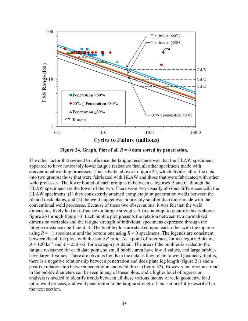
Because the original hypothesis guiding the work assumed penetration had an influence on fatigue resistance, all of the R = 0 data are presented in S-N format in figure 24. The data were divided into three groups: penetration greater than 80 percent, penetration between 80 and 60 percent, and penetration less than 60 percent. The group representing specimens with penetration less than 60 percent demonstrated higher fatigue resistance with a lower bound just above category B. The other two groups of specimens had lower bound resistance around category C. This may indicate that penetration is not as influential on fatigue resistance as originally thought when the research began.

1

10

100

0.1 1.0 10.0 100.0

LSS

Ran

ge a

t Wel

d R

oot (

ksi)


Root Failures (R= -1)

Root Failure (95% confidence)

Cat B

Cat C

Cat D

43

Figure 24. Graph. Plot of all R = 0 data sorted by penetration.

The other factor that seemed to influence the fatigue resistance was that the HLAW specimens appeared to have noticeably lower fatigue resistance than all other specimens made with conventional welding processes. This is better shown in figure 25, which divides all of the data into two groups: those that were fabricated with HLAW and those that were fabricated with other weld processes. The lower bound of each group is in between categories B and C, though the HLAW specimens are the lower of the two. There were two visually obvious differences with the HLAW specimens: (1) they consistently attained complete joint penetration welds between the rib and deck plates, and (2) the weld nugget was noticeably smaller than those made with the conventional weld processes. Because of these two observations, it was felt that the weld dimensions likely had an influence on fatigue strength. A first attempt to quantify this is shown figure 26 through figure 33. Each bubble plot presents the relation between two normalized dimension variables and the fatigue strength of individual specimens expressed through the fatigue resistance coefficient, A. The bubble plots are stacked upon each other with the top one using R = −1 specimens and the bottom one using R = 0 specimens. The legends are consistent between the all the plots with the same R-ratio. As a point of reference, for a category B detail, A = 120 ksi3 and A = 250 ksi3 for a category A detail. The area of the bubbles is scaled to the fatigue resistance for each data point, so small bubble area have low A values, and large bubbles have large A values. There are obvious trends in the data as they relate to weld geometry, that is, there is a negative relationship between penetration and deck plate leg length (figure 28) and a positive relationship between penetration and weld throat (figure 32). However, no obvious trend in the bubble diameters can be seen in any of these plots, and a higher level of regression analysis is needed to identify trends between all these various factors of weld geometry, load ratio, weld process, and weld penetration to the fatigue strength. This is more fully described in the next section.

44

Figure 25. Graph. Plot of all fatigue data differentiated by welding process.

45

Figure 26. Graph. Relation between rib and deck plate leg sizes at R = −1.

Figure 27. Graph. Relation between rib and deck plate leg sizes at R = 0.

Figure 28. Graph. Relation between weld penetration and deck plate leg size at R = −1.

Figure 29. Graph. Relation between weld penetration and deck plate leg size at R = 0.

0.0

0.3

0.6

0.9

1.2

1.5

1.8

0.0 0.3 0.6 0.9 1.2 1.5 1.8

h/d 4

(nor

mal

ized

leg

dim

ensi

on o

n rib

pla

te)

d1/d4 (normalized leg dimension on deck plate)

A = 250 ksi3

A = 500 ksi3

A = 1000 ksi3

A = 2000 ksi3

0.0

0.3

0.6

0.9

1.2

1.5

1.8

0.0 0.3 0.6 0.9 1.2 1.5 1.8

h/d 4

(nor

mal

ized

leg

dim

ensi

on o

n rib

pla

te)


A = 188 ksi3

A = 375 ksi3

A = 750 ksi3

A = 1500 ksi3

0.0

0.3

0.6

0.9

1.2

1.5

1.8

0.0 0.3 0.6 0.9 1.2 1.5 1.8

d 2/d

4(n

orm

aliz

ed w

eld

pene

tratio

n)


A = 250 ksi3

A = 500 ksi3

A = 1000 ksi3

A = 2000 ksi3

0.0

0.3

0.6

0.9

1.2

1.5

1.8

0.0 0.3 0.6 0.9 1.2 1.5 1.8

d 2/d

4(n

orm

aliz

ed w

eld

pene

tratio

n)


A = 188 ksi3

A = 375 ksi3

A = 750 ksi3

A = 1500 ksi3

46

Figure 30. Graph. Relation between throat and deck plate leg sizes at R = −1.

Figure 31. Graph. Relation between throat and deck plate leg sizes at R = 0.

Figure 32. Graph. Relation between weld penetration and throat at R = −1.

Figure 33. Graph. Relation between weld penetration and throat at R = 0.

0.0

0.3

0.6

0.9

1.2

1.5

1.8

0.0 0.3 0.6 0.9 1.2 1.5 1.8

t/d4

(nor

mal

ized

thro

at)


A = 250 ksi3

A = 500 ksi3

A = 1000 ksi3

A = 2000 ksi3

0.0

0.3

0.6

0.9

1.2

1.5

1.8

0.0 0.3 0.6 0.9 1.2 1.5 1.8

t/d4

(nor

mal

ized

thro

at)


A = 188 ksi3

A = 375 ksi3

A = 750 ksi3

A = 1500 ksi3

0.0

0.3

0.6

0.9

1.2

1.5

1.8

0.0 0.3 0.6 0.9 1.2 1.5 1.8

d 2/d

4(n

orm

aliz

ed w

eld

pene

tratio

n)

t/d4 (normalized throat)

A = 250 ksi3

A = 500 ksi3

A = 1000 ksi3

A = 2000 ksi3

0.0

0.3

0.6

0.9

1.2

1.5

1.8

0.0 0.3 0.6 0.9 1.2 1.5 1.8

d 2/d

4(n

orm

aliz

ed w

eld

pene

tratio

n)

t/d4 (normalized throat)

A = 188 ksi3

A = 375 ksi3

A = 750 ksi3

A = 1500 ksi3

47

REGRESSION ANALYSIS OF FATIGUE RESULTS

Fatigue tests were performed on specimens consisting of differing geometries using two different load ratios. Furthermore, specimen weld dimensions varied from test to test. Thus, there were several possible sources of variation in fatigue resistance for the tested specimens. A statistical regression analysis was conducted to determine which factors and quantitative variables best explained the specimen-to-specimen variation in fatigue resistance. The primary objective of the regression analysis was to derive a parametric predictive model that could be used to calculate the fatigue resistance of welded orthotropic details similar to those examined in this study. Determining which test variables are most strongly correlated to fatigue performance allows the possibility of less uncertainty in the classification of the proper fatigue design category for welded orthotropic details. As mentioned previously, the fact that small specimens were used to obtain fatigue resistance data was not considered as part of the analysis. All analysis was conducted using the R statistical computing environment.(11)

STATISTICAL DATASET

Table 18 summarizes the observed dataset variables that were considered in the regression analysis. Of the 12 variables, 5 were factor variables (i.e., categorical variables), and 7 were continuous variables. The range column gives the set of possible values for each variable. The meanings of the weld dimension variables are illustrated in appendix B and appendix C.

Table 18. Statistical data variables.

Variable Type Range Load ratio Factor {−1, 0} Failure mode Factor {Deck, Rib, Root} Geometry Factor {Type 1, Type 2, Type 3} Laser welded Factor {Laser, Non-Laser} Root gap opening Factor {Open, Closed} Cycles Continuous ≥ 0 Stress range Continuous ≥ 0 d1 Continuous ≥ 0 d2 Continuous [0,1] d4 Continuous ≥ 0 h Continuous ≥ 0 t Continuous ≥ 0

With the exception of some of the laser-welded specimens, the dataset consisted of complete observations. As shown in appendix C, weld geometry measurements were available for only 10 of the laser welded specimens. One of the primary goals in building a predictive regression model was to uncover possible relationships between weld geometry and fatigue resistance. Thus, the laser-welded specimens without weld measurements were excluded from the

48

regression analysis. While it is possible to impute values for the specimens without measurements in some way using the specimens for which measurements were available, this was avoided so as not to diminish any relationships between geometry and resistance.

The dataset originally consisted of 144 specimens after excluding runouts. Eliminating laser specimens without weld geometry measurements removed 28 specimens from the analysis dataset. In addition, specimens GM8-3 and SA8-9 were removed from the dataset for statistical analysis purposes after data preprocessing, leaving 114 specimens. The fatigue resistance of specimen GM8-3 was significantly higher than for the remaining specimens with the same load ratio. Examination of the data in table 5 shows that this specimen was loaded at 20.16 ksi for 18,253,515 cycles prior to failure. This is the third-lowest stress range amongst all of the specimens tested from that series. The only two specimens with a lower stress range were runout specimens. It is likely that the loading conditions for specimen GM8-3 were within the transition region in going from log-linear S-N behavior to infinite fatigue life behavior. As is the case with the runout specimens, banishing the specimen from the dataset results in more conservative fatigue resistance predictions.

It can be seen in table 6 that specimen SA8-9 had a particularly low fatigue resistance relative to other specimens. Exploratory data analysis revealed that the weld dimension along the rib plate, h, was noticeably lower than the measured values for other specimens relative to the specimen rib thickness. It was suspected there may have been a transcription error with this specimen, and it was excluded from the dataset to prevent it from masking relationships. All plots and analysis moving forward in this chapter correspond to the dataset after removal of the aforementioned specimens.

Regression Function

The S-N fatigue life model for welded steel bridge details implicitly assumes that there is a linear relationship in log-log space between the number of cycles to failure and the applied stress range when the stress range is above some specified fatigue threshold. In non-log space, this amounts to saying that the number of cycles to failure for a welded steel bridge detail is proportional to the stress range raised to some power. Thus, fatigue resistance can be thought of as a product of the underlying process parameters in non-log space. The error component in this case can be assumed to be a positive multiplicative value as opposed to additive. With this in mind, the regression function used to model the experimental fatigue resistance coefficients in its most general non-log form is shown in figure 34.

Figure 34. Equation. General regression function.

Where:

Ai = Fatigue resistance coefficient of the ith test specimen. = Base fatigue resistance coefficient (ksi3).

𝐴𝐴𝑖𝑖 = ��̃�𝐴�𝑥𝑥𝑖𝑖𝑖𝑖 𝛽𝛽𝑖𝑖𝑝𝑝

𝑖𝑖=1

�𝜀𝜀𝑖𝑖

�̃�𝐴

49

xij = Value of the jth predictor variable for the ith test specimen. j = Coefficient corresponding to the jth predictor variable.

i = Random error component (> 0) for the ith test specimen.

Thus, the fatigue resistance coefficient was modeled as the product of some base resistance coefficient and a series of p modifiers that depend on the observed experimental variables. Taking the base 10 log of both sides of the equation given in figure 34 gives the result shown in figure 35.

Figure 35. Equation. Linear regression function.

It is seen from the form of this equation that the regression function is a linear model in log-space. The fatigue resistance coefficient for a test specimen was taken as the product of the number of cycles to failure and the cube of the calculated hot spot stress range as is consistent with the fatigue provisions for welded steel bridge details included in AASHTO BDS. Thus, it was implicitly assumed that the number of cycles to failure for a test specimen is inversely proportional to the cube of the corresponding stress range.

It should be noted that the value of the base fatigue resistance coefficient depends on relative factor levels should any factor variables be included as predictors in the model. Non-reference factor variable levels were coded in standard non-log space as either 1 if not applicable or 10 if applicable, corresponding to values of either 0 or 1, respectively, in the additive log-space regression function of figure 35. Thus, the presence of a factor variable in the model amounts to increasing or decreasing the fatigue resistance coefficient by a specified constant multiplicative factor in standard space when applicable. Also, note that if the random error component follows a lognormal distribution, then the value in parentheses of the equation in figure 34 represents the conditional median value of the fatigue resistance coefficient given the specified values of the predictor variables.

Cross-Validation

Regression analysis involves determining the unknown model parameters for the chosen function that minimize some specified error criterion for the dataset that was used in the analysis or the training set. The average error of a fitted regression model corresponding to the training set observations will tend to be lower than the actual error that would be observed when using the model to predict a response for new and unseen observations that were not part of the training set. Thus, a different selection criterion other than training error is necessary to select a model that minimizes prediction error for unseen observations that were not part of the model fitting process.

For the fatigue resistance analysis, repeated tenfold cross-validation was used as a means to select the optimal model that minimizes prediction error. Tenfold cross-validation involves randomly splitting the statistical dataset observations into 10 approximately equally sized subset splits. A candidate regression model is then fit 10 times to the data, leaving a different split out

𝛽𝛽 𝜀𝜀

log10 𝐴𝐴𝑖𝑖 = log10 �̃�𝐴 + �𝛽𝛽𝑖𝑖 log10 𝑥𝑥𝑖𝑖𝑖𝑖

𝑝𝑝

𝑖𝑖=1

+ log10 𝜀𝜀𝑖𝑖

50

each time. The excluded split is used to estimate the prediction error of the candidate model. The cross-validation errors for the model are then averaged over all splits. The average errors can be used to discriminate between different candidate models that were fit using different model parameters. Five tenfold repetitions were used in calculating cross-validation errors for a total of 50 model fits corresponding to a given candidate regression model. The calculated average error for a specific training/test split was naively assumed to be independent of the average error calculated using some other split. In the case of standard linear regression, different candidate models correspond to models containing different combinations of the predictor variables.

Standard Least Squares Linear Regression

Using standard least squares linear regression, the values of the predictor variable coefficients in the equation of figure 35 are determined by minimizing the sum of the squared model residuals over some training set of observations, given by the equation shown in figure 36.

Figure 36. Equation. Standard least squares regression error function.

The model-tuning parameter to be determined by cross-validation in this case was the number of predictor variables to be included in the regression function. Table 19 lists the predictor variables considered in fitting the least squares model. For factor variables, the reference level used in the regression analysis is listed in parentheses in the “Type” column. The levels for each factor variable were given in table 18. Note that for the factor variable coding scheme used, the number of candidate predictors for a factor variable is always one less than the number of corresponding factor levels; as mentioned previously, the reference level given in parentheses is implicitly included as part of the base fatigue resistance coefficient of the regression function. Weld dimension predictor variables were normalized by the d4 dimension, which is strongly related to the thickness of the orthotropic rib plate. This was done so that the weld dimension variables would be independent of the overall structural geometry between different specimens. For example, one might expect that a 1/4-inch weld would experience different stress gradients in a structural configuration where the rib plate was 1 inch thick compared to a configuration where the rib plate was only 1/2 inch thick. The d3 dimension and the d5 dimension were excluded because they are linear combinations of the weld dimensions that are shown in the table and result in near perfect correlations with the other dimensions even after the log transformation.

𝐸𝐸𝐿𝐿𝐿𝐿 = ��log10 𝐴𝐴𝑖𝑖 − log10 �̃�𝐴 −�𝛽𝛽𝑖𝑖

𝑝𝑝

𝑖𝑖=1

log10 𝑥𝑥𝑖𝑖𝑖𝑖 �

2

𝑖𝑖

51

Table 19. Standard regression predictor variables.

Variable Type Load ratio Factor (−1) Failure mode Factor (Deck) Geometry Factor (Type 1) Laser Factor (Laser) Gap Factor (Closed) d1/d4 Continuous d2/d4 Continuous h/d4 Continuous t/d4 Continuous (Failure mode):(d1/d4) Factor-continuous interaction (Deck:d1/d4) (Failure mode):(d2/d4) Factor-continuous interaction (Deck:d2/d4) (Failure mode):(h/d4) Factor-continuous interaction (Deck:h/d4) (Failure mode):(t/d4) Factor-continuous interaction (Deck:t/d4) (Load ratio):(d1/d4) Factor-continuous interaction (Load ratio = −1:d1/d4) (Load ratio):(d2/d4) Factor-continuous interaction (Load ratio = −1:d2/d4) (Load ratio):(h/d4) Factor-continuous interaction (Load ratio = −1:h/d4) (Load ratio):(t/d4) Factor-continuous interaction (Load ratio = −1:t/d4)

Even though deck plate thickness did vary in the testing matrix, this was not exclusively considered in the regression because it was inherently coupled to the stress range calculation.

In addition to the factor variables and normalized weld dimensions, interaction variables between each normalized weld dimension together with the failure mode and load ratio were considered. This was done to account for the possibility that one weld dimension may be of greater importance in the presence of a particular failure mode or load ratio in comparison to other dimensions. Including such an interaction in the model would result in a change of the weld dimension exponent as shown in the equation of figure 34 given the occurrence of the particular failure mode or load ratio under consideration in the interaction.

Forward stepwise selection with a slight modification to satisfy the principle of hierarchy was used to select the best model for each given model size and a given training/test cross-validation split. The principle of hierarchy specifies that when an interaction term is included in a regression model, it should also be the case that the main effects of the interaction are included in the model to preserve the intended meaning of the interaction. Thus, if it were determined by forward selection for a given model size that the best model included an interaction term, a check was made to insure that the main effect terms were already included in the model. If this was not the case, the next best model of the intended size was selected, and the check repeated until the principle of hierarchy was satisfied.

52

Figure 37 shows a plot of the average cross-validation mean square errors (MSEs) as determined by the model fitting procedure. The error bars in the plot represent one standard error above and below the mean cross-validation error. It is likely that the standard errors shown are larger in reality because of the implicit assumption of independence in the calculation. The zero variable model, or null model, corresponds to the case where only the base fatigue resistance coefficient is included in the regression function. This is equivalent to predicting the value of the fatigue resistance coefficient for a test specimen using the geometric mean of all observed resistance coefficients used to fit the model.

Figure 37. Graph. Standard regression cross-validation error.

The final model predictor variable coefficients in log-space found using the aforementioned forward selection process applied to the full statistical dataset are given in table 20. The lowest cross-validation error occurs when seven predictor variables are included in the model, not including the base fatigue resistance coefficient. Thus only models with seven variables or less are shown in the table. Also shown are the average cross-validation MSEs together with the corresponding standard errors for the given number of variables used. While a model with seven predictor variables results in the lowest cross-validation error, it can be seen that the cross-validation error for a model containing four predictor variables falls within the standard error bounds for the seven variable model. Thus it was decided to use the less complex regression function containing three predictor variables as the final selected predictive model determined using standard regression. As can be seen in table 20, the four most influential predictors ranked in the order that they enter the model are load ratio, weld leg length along the deck plate, weld root failure, and weld penetration. The four-variable model can be expressed as shown in figure 38.

53

Table 20. Final model regression coefficients by forward selection.

Model Variables

Cross- Validation

MSE

Standard Error of

MSE

Load Ratio = 0a d1/d4

Weld Root

Failureb d2/d4

Root Failure:

d1/d4b

Rib Failure

Rib Failure:

d1/d4b

0 0.109 0.00561 10.6 NA NA NA NA NA NA NA 1 0.0654 0.00308 10.7 −0.447 NA NA NA NA NA NA 2 0.0601 0.00327 10.8 −0.450 0.661 NA NA NA NA NA 3 0.0475 0.00247 10.9 −0.524 0.884 −0.356 NA NA NA NA 4 0.0427 0.00247 11.2 −0.513 1.44 −0.414 0.960 NA NA NA 5 0.0417 0.00257 11.2 −0.514 1.51 −0.416 1.02 −3.12 NA NA 6 0.0399 0.00294 11.2 −0.495 1.42 −0.382 0.969 −3.04 0.118 NA 7 0.0390 0.00297 11.2 −0.494 1.476 −0.389 −0.985 −3.09 0.0762 −1.934

a value already includes the reference level of load ratio = −1 as shown in table 19. b value already includes the reference level of failure mode = deck as shown in table 19. NA = Not applicable.

𝑨𝑨�

�̃�𝐴 �̃�𝐴

54

Figure 38. Equation. Least squares regression final predictive model.

Where:

1 = 1 for tension-only loading, 0 for load reversals. α 2 = 1 for weld root failure, 0 otherwise. After further simplification, the least squares regression final predictive model is shown in figure 39.

Figure 39. Equation. Simplified least squares regression final predictive model.

The model specifies that full load reversals (load ratio = −1) correspond to fatigue resistances in the test specimens approximately three times greater in an average sense than tension-only specimens (load ratio = 0) assuming that other variables remain constant. It is also seen that there is a reduced fatigue resistance coefficient for weld root failures in comparison to other failure modes. Note that the model as shown is somewhat deceptive in this regard as a result of the fact that weld root failures occurred only in the presence of load reversals, so the two reduction factors in the model do not apply simultaneously for any of the specimens tested. Finally, it can be seen that the fatigue resistance is given as a function of the d1

weld dimension as well as weld penetration. For both variables, there is positive correlation with fatigue resistance. However, it should be noted that the d1 dimension has a higher exponent and is generally not restricted to values less than or equal to 1 as is the weld penetration. Thus, for the experimental specimens, the d1 dimension is a more influential predictor of fatigue resistance than is the weld penetration. Furthermore, as the normalized d1 dimension increases, the weld penetration generally tends to decrease. Thus, it makes sense to specify design requirements for the weld leg dimension.

A normal probability plot of the deleted residuals for the final model fit is shown in figure 40. The residuals were externally studentized and segregated by load ratio: squares for R = −1 and circles for R = 0. It can be seen that the residuals for the four-variable model exhibit some right skewness with a mean approximately equal to zero. It is also seen that the tails of the residual distribution are dominated by specimens that were subjected to load reversals. The ramifications of the residual distribution in deriving design guidelines are discussed in the next section.

log10 𝐴𝐴 = 11.2 − 0.513𝛼𝛼1 + 1.44 log10 �𝑑𝑑1

𝑑𝑑4� − 0.414𝛼𝛼2 + 0.960 log10 �

𝑑𝑑2

𝑑𝑑4�

α

𝐴𝐴 = 1585𝑒𝑒8 𝑘𝑘𝑘𝑘𝑖𝑖3 ∙ 0.307𝛼𝛼1 ∙ 0.385𝛼𝛼2 ∙ �𝑑𝑑1

𝑑𝑑4�

1.44

�𝑑𝑑2

𝑑𝑑4�

0.960

55

Figure 40. Graph. Normal probability plot of standard regression studentized residuals.

DESIGN RECOMMENDATIONS

It was shown in figure 40 that the standard regression model residuals exhibit right skewness in log-space. Figure 41 shows a histogram of the final fitted model residuals. Also shown on the plot are two different continuous normal distributions. The solid line distribution illustrates a normal distribution with location parameter equal to zero and scale parameter equal to the standard deviation of the fitted model residuals. As mentioned previously, the expected value of the MSE as calculated on the training set potentially gives an overly optimistic estimate for the actual error that would be observed when using the model to predict values for new observations. Thus, for design purposes, it is prudent to use a larger-scale parameter than is given by the standard deviation of the model residuals. The dashed line normal distribution shown in figure 41 is the distribution obtained when using the cross-validation MSE to calculate the scale parameter. The tails of the distribution are larger than in the previous case. While the distribution does not precisely capture the small amount of skewness in the residual distribution, the tails of the distribution should provide a sufficient lower bound estimate for design purposes. Furthermore, if design guidelines are derived assuming a zero load ratio, most of the extreme residuals shown in the histogram become irrelevant, as was illustrated in figure 40. Thus, for design purposes, model predictions were assumed to have a lognormal distribution as represented by the green dashed line curve in figure 41 and a zero load ratio. The assumption of a zero load ratio will become clear in the derivations that follow.

56

Figure 41. Histogram. Distribution of model residuals.

As is consistent with current fatigue design practice, a lower bound fatigue resistance for the experimental specimens can be expressed as the resistance corresponding to two standard deviations below the mean in log-space. The cross-validation standard deviation estimate (square root of the MSE) for the standard regression model was 0.207 in log-space. Using this as an estimate of the true prediction error of fatigue resistance for the standard regression model gives for a design resistance coefficient as shown in figure 42.

Figure 42. Equation. Design fatigue resistance coefficient.

All variables in the equation are as defined for the equation in figure 38. As mentioned previously, it can be conservatively assumed for design purposes that the load ratio will be equivalent to the worst case, tension-only load ratio loading. Revising the equation to account for this assumption and reverting out of log-space gives the result shown in figure 43.

Figure 43. Equation. Simplified design fatigue resistance coefficient.

log10 𝐴𝐴𝐷𝐷 ≤ 11.2 − 0.513𝛼𝛼1 − 0.414𝛼𝛼2 + 1.44 log10 �𝑑𝑑1

𝑑𝑑4� + 0.960 log10 �

𝑑𝑑2

𝑑𝑑4� − 2 ∙ 0.207

𝐴𝐴𝐷𝐷 ≤ (187𝑒𝑒08 𝑘𝑘𝑘𝑘𝑖𝑖3) ∙ 0.385𝛼𝛼2 ∙ �𝑑𝑑1

𝑑𝑑4�

1.44

�𝑑𝑑2

𝑑𝑑4�

0.960

57

Regarding the occurrence of weld root failures, examination of the statistical dataset shows the following:

• All weld root failures occurred under load reversals (R = −1). • Fourteen of the sixteen weld root failures occurred in conjunction with an open root gap.

Implicit in the inequality is the assumption of a zero load ratio, therefore it would be conservative to simply use the inequality of figure 44 with the weld root term eliminated. The second observation can be used as a basis for a fabrication guideline specifying that rib-to-deck welds be fabricated with closed root gaps in the welded condition. A final design inequality is shown in figure 44.

Figure 44. Equation. Design weld-dimension inequality.

There is discretion to choose a value for AD, though based on the presentation in figure 19 and figure 20, categories B or C would be most prudent. However, as the first term in figure 44 has a denominator of 187e08 ksi3 indicates the fitted model for design is halfway between category B (120e08 ksi3) and category A (250e08 ksi3). For the sake for further presentation of the design inequality, the first term in figure 44 can be represented by a constant, k, and results in the equation shown in figure 45.

Figure 45. Equation. Final design weld-dimension inequality.

The value of the constant, k, in the inequality is given in table 21 for fatigue design categories A–C.

Table 21. Weld leg design coefficient.

Design Category k

A 1.35 B 0.630 C 0.222

Figure 46 graphically illustrates the experimental data and the derived weld design inequality of figure 45. The data are plotted with the weld penetration (d2/d4) on the y-axis, and the normalized d1-dimension is plotted on the x-axis. The dashed lines represent the boundaries for fatigue design by category as given by the weld design inequality. The sizes of the plotted points are representative of the measured fatigue resistance coefficients as specified in the corresponding legends. As per the equation in figure 39, the fatigue resistances should increase in moving up

�𝐴𝐴𝐷𝐷

187𝑒𝑒08 𝑘𝑘𝑘𝑘𝑖𝑖3�1.04

∙ �𝑑𝑑1

𝑑𝑑4�−1.50

≤ �𝑑𝑑2

𝑑𝑑4�

𝑘𝑘 �𝑑𝑑1

𝑑𝑑4�−1.50

≤ �𝑑𝑑2

𝑑𝑑4�

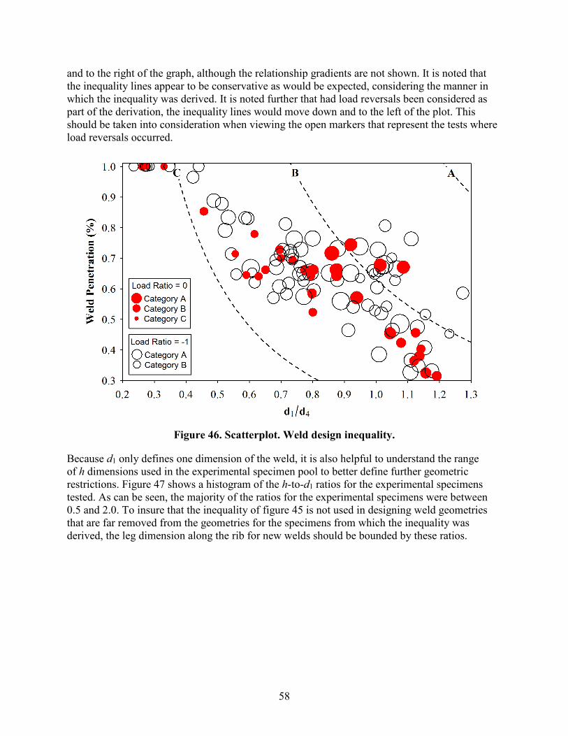
58

and to the right of the graph, although the relationship gradients are not shown. It is noted that the inequality lines appear to be conservative as would be expected, considering the manner in which the inequality was derived. It is noted further that had load reversals been considered as part of the derivation, the inequality lines would move down and to the left of the plot. This should be taken into consideration when viewing the open markers that represent the tests where load reversals occurred.

Figure 46. Scatterplot. Weld design inequality.

Because d1 only defines one dimension of the weld, it is also helpful to understand the range of h dimensions used in the experimental specimen pool to better define further geometric restrictions. Figure 47 shows a histogram of the h-to-d1 ratios for the experimental specimens tested. As can be seen, the majority of the ratios for the experimental specimens were between 0.5 and 2.0. To insure that the inequality of figure 45 is not used in designing weld geometries that are far removed from the geometries for the specimens from which the inequality was derived, the leg dimension along the rib for new welds should be bounded by these ratios.

59

Figure 47. Histogram. Frequency of h-to-d1 ratio in experimental specimens.

Finally, the design parameter, k, used in the previous discussion provides leeway to selection of fatigue resistance to be categories C or B. Selecting one versus the other effectively changes minimum weld size and penetration per the design inequality. Considering the S-N plot shown in figure 22, category C would be a good candidate. Another reason to use category C is to avoid the conundrum of constant amplitude fatigue threshold (CAFT) with LSS analysis as the category C CAFT is 10 ksi. To illustrate the difference, figure 48 shows the variation in required weld sizes when using the category C design versus the category B design using the same rib and deck plate geometries with an assumed 60 percent penetration requirement. The design inequality was used to determine the required minimum d1 dimension, and then h dimensions of 0.6d1 and 2.0d1 were drawn to show the bounds. Therefore, the minimum weld is filled with a cross-hatch pattern and the maximum weld with a hatched pattern. While category B design would allow for use of higher stress ranges in the design model, this comes at the expense of a larger weld as shown in figure 48.

From the stance of this research, there should be no problem making the d1 dimension larger than output from the design inequality, though the largest d1/d4 ratio of all the specimens was approximately 1.30. This would be helpful because the minimum diagrammatic welds shown in figure 48 may not be welds that are efficient, or even feasible, and other criteria may control such as maintaining a throat dimension equal to the rib thickness. The design inequality allows the engineer to assume the rib-to-deck plate weld has category C resistance in design and allows them flexible detailing requirements in terms of weld penetration and deck plate leg length to ensure that category C resistance is delivered.

60

Figure 48. Illustration. Comparison of minimum weld dimensions for categories C or B

fatigue design.

61

CONCLUSIONS AND RECOMMENDATIONS

This research was performed to develop design and detailing recommendations to make the rib-to-deck weld for orthotropic decks more friendly for fabrication. At the time the research began, the current standard for this detail was an 80-percent minimum weld penetration requirement with an initial tight fit and no tolerance for melt- or blow-through in the as-welded condition. As an example, the difference between 80- and 100-percent penetration given a 5/16-inch rib wall thickness is quite small, and further coupling with a fit-up tolerance not to exceed 0.01 inch makes the weld prohibitively difficult to fabricate. Variations in the fit-up tolerance between the rib and deck can easily result in melt-through or blow-through when attempting to achieve nearly full penetration, especially if the fit-up between the plates is not consistent.

A number of variables were hypothesized to affect the fatigue resistance of this detail, and it was not possible to test a statistically significant population of full-size decks for all of the variables. Therefore, a full-scale, small-specimen fatigue testing protocol was developed to investigate the fatigue resistance of this detail by slicing an individual welded panel into numerous individual specimens. These tests are a cost-effective way to rapidly generate large amounts of data and study the significance of weld procedure variables.

Overall, the study determined that the primary factor in the fatigue resistance of the rib-to-deck weld is its geometry. Welds with larger leg dimensions along the deck plate perform better in fatigue, and, as this leg dimension increases, there is a commensurate decrease in the required penetration. Welds with penetration varying from 40 to 100 percent can be designed assuming a level 3 fatigue analysis with category C fatigue resistance provided the weld leg dimension meets minimum size requirements.

RECOMMENDATIONS

The stress analysis used throughout this report was consistent with a level-3 design procedure. The following recommendations are proposed for consideration and potential adoption into the Federal Highway Administration Manual for Design, Construction, and Maintenance of Orthotropic Steel Deck Bridges and the seventh edition of the AASHTO LRFD Bridge Design Specifications; however, no consideration of level-1 or level-2 design procedures was considered:(10,8)

1. Weld geometry must be made to satisfy the inequality that penetration shall be greater than 0.222(d1/d4) −1.50, where d1/d4 is the normalized leg weld dimension along the deck plate. Therefore, two options exist: (1) pick a target penetration value and calculate minimum leg size or (2) select a leg size and calculate a minimum penetration. Either way will produce welds that exceed category C design resistance.

2. The ratio of weld leg dimensions, h-to-d1, shall be between 0.6 and 2.0, and d1/d4 shall be between 0.40 and 1.30. This is to maintain consistency with the specimens tested and reported herein.

3. Qualification shall be performed to ensure welding procedures produce production welds with a closed root condition. The closed root condition is not defined as being fused; it is

62

merely the notion that the inside rib corner is visibly in close contact with the deck plate. Provided a closed root condition is maintained, root failures should be suppressed.

4. The current pre-welded fit-up gap of 0.020 inch is considered sufficient. For the two panels fabricated with 0.020-inch fit-up gaps, the gap mostly closed across the whole length of panel from weld shrinkage, and there were no weld root failures from these populations of specimens1. Some evidence was presented that 1/32-inch gaps can also close, though they were largely not fatigue tested, and the 0.020-inch recommendation is considered conservative.

FUTURE RESEARCH

The full-scale small-specimen test(s) should be developed into a standardized testing protocol that can evaluate the rib-to-deck weld prior to fabrication. Most bridge owners already require fabricators to produce full-scale mock-ups of rib-to-deck weldments as a qualification test prior to fabrication. It would be relatively inexpensive to section some fatigue test specimens from the mock-ups, and it takes about 1 to 2 d to perform a fatigue test. Such a qualification test can be useful to allow fabricators leeway for efficient design of this weldment.

Currently, the LSS method is limited to weld toes only. The reason is the LSS method assumes that the disparity between the predicted structural stress and the actual stress is uniform throughout all weld toes. Hence, the fatigue resistance for all weld toes follows the same S-N curve. However, this assumption no longer holds for weld roots because the notch effect is much more severe. This is especially true for open root gaps because they create crack-like defects whose fatigue resistance highly depends on the local geometry and is thus difficult to capture by a single S-N curve. A more comprehensive methodology to determine the fatigue resistance from the root of partial penetration welds will be a useful advance in practice.

The use of the AASHTO category C resistance curve has been shown to work well with the LSS method in the finite life regime where all stress cycles exceed the fatigue threshold. However, it is unknown if the 10-ksi fatigue threshold for this category applies to the rib-to-deck weld. Additional testing is recommended at lower stress ranges to determine the proper threshold for this weldment. This will enable design of orthotropic decks for infinite fatigue life.

More work is needed to correlate the full-scale small-specimen tests to full-scale testing and in-service performance of orthotropic decks. The full-scale, small specimen tests should be considered to supplement any future tests of orthotropic decks.

There is one exception to this statement. Specimen UB-2 was reported to have a closed root condition and did fail in the weld root under reversal loading. However, a macroetch of that weld was not provided, and it is possible that this may have been reported as a closed condition because that was the intent of the UB panel, but the actual welded condition may have been open.

63

APPENDIX A. SECTIONING OF PANELS INTO SPECIMENS

Figure 49 through figure 62 in this appendix show how individual panels were cut into specimens for the first series of panels that were machined at TFHRC. In the later stages of the project, the fabricator was paid to section the panels with a bandsaw, and it is presumed that specimens were ordered sequentially along the length of the panel.

Units = Inches.

Figure 49. Illustration. GM8 series panel.

Units = Inches.

Figure 50. Illustration. SA8 series panel.

Units = Inches.


64

Units = Inches.


Units = Inches.


Units = Inches.

Figure 54. Illustration. FIL series panel.

65

Units = Inches.

Figure 55. Illustration. LP1 series panel.

Units = Inches.


66

Units = Inches.


Units = Inches.

Figure 58. Illustration. OB series panel.

Units = Inches.

67

Figure 59. Illustration. UB series panel.

Units = Inches.

Figure 60. Illustration. OG1 series panel.

68

Units = Inches.

Figure 61. Illustration. OG2 series panel.

Units = Inches.

Figure 62. Illustration. W series panel.

69

APPENDIX B. WELD DIMENSIONS

This appendix presents the data associated with all measurements taken of weld cross sections from some panel series. These measurements were not taken on any of the OG series panels. Measurements for the laser welded specimens are in appendix C. The weld location syntax used in table 22 through table 30 is shown in figure 63. Weld locations 1 and 2 are on one machined face of the specimen, and locations 3 and 4 are on the opposing machined face. Locations 1 and 3 are on the side with the dominant fatigue crack size because both welds sometimes cracked simultaneously. The exception to this rule is for the W series specimens in table 30, where a table footnote is used to denote the side with the dominant fatigue crack. In addition, the W series specimens were only etched on one face of each specimen in lieu of both sides for the majority of the specimens. This was done to save time because the unetched face of one specimen abuts the etched face of the neighboring specimen. The remaining column headings in this appendix’s tables present the measurements recorded as shown in figure 64.

Figure 63. Schematic. Denotation of weld locations.

70

Figure 64. Schematic. Measured dimensions.

Where:

d1 = Weld length along the deck plate. d2 = Weld penetration along the deck plate. d3 = Size of the gap behind the weld. d4 = Projected width of rib on deck plate. d5 = Length from weld toe to inside edge of rib. d2/d4 = Percentage of the weld penetration. h = Total weld length along the rib plate. h1 = Weld length along the rib plate. h2 = Face gap. t = Actual weld throat size, defined as the distance from the weld root to the nearest point on the curved weld surface.

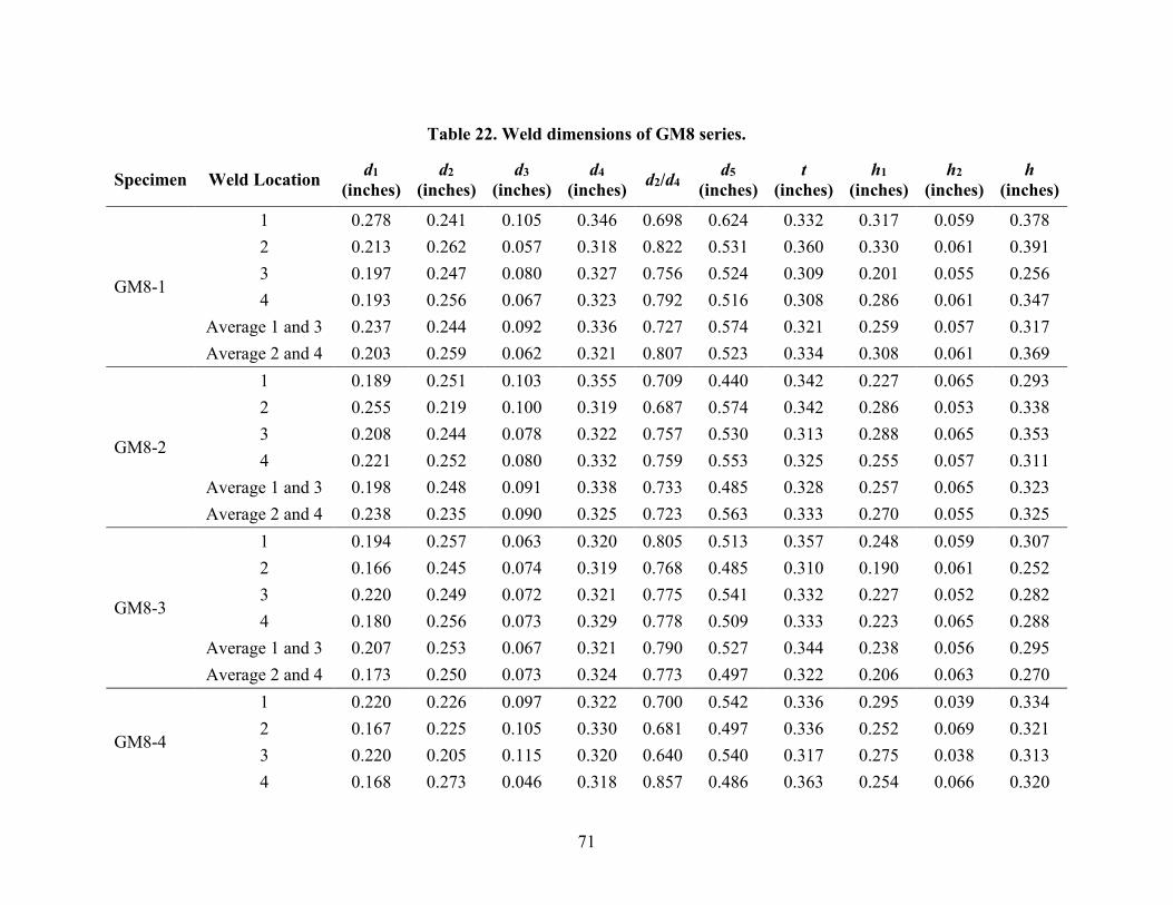
71

Table 22. Weld dimensions of GM8 series.

Specimen Weld Location d1 (inches)

d2 (inches)

d3 (inches)

d4 (inches) d2/d4 d5

(inches) t

(inches) h1

(inches) h2

(inches) h

(inches)

GM8-1

1 0.278 0.241 0.105 0.346 0.698 0.624 0.332 0.317 0.059 0.378 2 0.213 0.262 0.057 0.318 0.822 0.531 0.360 0.330 0.061 0.391 3 0.197 0.247 0.080 0.327 0.756 0.524 0.309 0.201 0.055 0.256 4 0.193 0.256 0.067 0.323 0.792 0.516 0.308 0.286 0.061 0.347

Average 1 and 3 0.237 0.244 0.092 0.336 0.727 0.574 0.321 0.259 0.057 0.317 Average 2 and 4 0.203 0.259 0.062 0.321 0.807 0.523 0.334 0.308 0.061 0.369

GM8-2

1 0.189 0.251 0.103 0.355 0.709 0.440 0.342 0.227 0.065 0.293 2 0.255 0.219 0.100 0.319 0.687 0.574 0.342 0.286 0.053 0.338 3 0.208 0.244 0.078 0.322 0.757 0.530 0.313 0.288 0.065 0.353 4 0.221 0.252 0.080 0.332 0.759 0.553 0.325 0.255 0.057 0.311


GM8-3

1 0.194 0.257 0.063 0.320 0.805 0.513 0.357 0.248 0.059 0.307 2 0.166 0.245 0.074 0.319 0.768 0.485 0.310 0.190 0.061 0.252 3 0.220 0.249 0.072 0.321 0.775 0.541 0.332 0.227 0.052 0.282 4 0.180 0.256 0.073 0.329 0.778 0.509 0.333 0.223 0.065 0.288


GM8-4

1 0.220 0.226 0.097 0.322 0.700 0.542 0.336 0.295 0.039 0.334 2 0.167 0.225 0.105 0.330 0.681 0.497 0.336 0.252 0.069 0.321 3 0.220 0.205 0.115 0.320 0.640 0.540 0.317 0.275 0.038 0.313 4 0.168 0.273 0.046 0.318 0.857 0.486 0.363 0.254 0.066 0.320

72


d2 (inches)

d3 (inches)


(inches) t

(inches) h1

(inches) h2

(inches) h

(inches)


GM8-5

1 0.217 0.252 0.053 0.305 0.828 0.522 0.347 0.222 0.052 0.275 2 0.154 0.274 0.043 0.317 0.863 0.471 0.348 0.226 0.061 0.286 3 0.220 0.246 0.063 0.309 0.797 0.529 0.347 0.245 0.052 0.297 4 0.170 0.248 0.065 0.313 0.792 0.483 0.327 0.206 0.061 0.267


GM8-6

1 0.162 0.265 0.061 0.325 0.814 0.487 0.350 0.224 0.063 0.286 2 0.157 0.254 0.076 0.330 0.770 0.411 0.352 0.256 0.055 0.311 3 0.185 0.262 0.079 0.340 0.768 0.526 0.350 0.222 0.068 0.290 4 0.216 0.195 0.135 0.330 0.592 0.545 0.304 0.230 0.056 0.286


GM8-7

1 0.181 0.268 0.047 0.315 0.851 0.496 0.357 0.251 0.056 0.308 2 0.196 0.256 0.055 0.312 0.822 0.508 0.332 0.206 0.063 0.269 3 0.195 0.255 0.060 0.316 0.809 0.511 0.341 0.235 0.057 0.292 4 0.165 0.267 0.054 0.321 0.831 0.486 0.334 0.222 0.062 0.284


GM8-8 1 0.244 0.219 0.106 0.325 0.674 0.569 0.338 0.243 0.054 0.297 2 0.174 0.255 0.072 0.326 0.780 0.500 0.339 0.241 0.062 0.303 3 0.233 0.229 0.093 0.322 0.711 0.554 0.351 0.274 0.055 0.329

73


d2 (inches)

d3 (inches)


(inches) t

(inches) h1

(inches) h2

(inches) h

(inches)

4 0.141 0.276 0.051 0.327 0.844 0.468 0.350 0.218 0.062 0.280 Average 1 and 3 0.238 0.224 0.099 0.323 0.693 0.562 0.344 0.259 0.054 0.313 Average 2 and 4 0.157 0.265 0.061 0.327 0.812 0.484 0.344 0.230 0.062 0.292

GM8-9

1 0.171 0.253 0.059 0.312 0.810 0.483 0.309 0.308 0.046 0.354 2 0.157 0.314 0.014 0.328 0.957 0.485 0.320 0.285 0.070 0.355 3 0.182 0.271 0.040 0.311 0.871 0.494 0.308 0.351 0.048 0.399 4 0.192 0.253 0.055 0.308 0.822 0.501 0.302 0.289 0.059 0.349


GM8-10

1 0.151 0.272 0.065 0.336 0.808 0.487 0.347 0.225 0.066 0.291 2 0.207 0.255 0.076 0.331 0.770 0.538 0.363 0.272 0.055 0.327 3 0.151 0.292 0.034 0.326 0.897 0.477 0.372 0.244 0.065 0.308 4 0.213 0.214 0.107 0.321 0.666 0.535 0.323 0.244 0.053 0.296


GM8-11

1 0.149 0.303 0.019 0.322 0.940 0.471 0.316 0.312 0.062 0.374 2 0.161 0.262 0.076 0.337 0.776 0.498 0.347 0.316 0.068 0.384 3 0.166 0.270 0.053 0.323 0.836 0.488 0.359 0.357 0.058 0.415 4 0.188 0.259 0.075 0.334 0.776 0.522 0.368 0.307 0.063 0.370


GM8-12 1 0.168 0.298 0.042 0.340 0.878 0.507 0.392 0.262 0.064 0.326 2 0.201 0.262 0.062 0.325 0.808 0.525 0.375 0.262 0.055 0.316

74


d2 (inches)

d3 (inches)


(inches) t

(inches) h1

(inches) h2

(inches) h

(inches)

3 0.180 0.298 0.042 0.340 0.878 0.507 0.392 0.232 0.059 0.291 4 0.229 0.241 0.085 0.326 0.738 0.554 0.349 0.276 0.050 0.326


GM8-13

1 0.134 0.308 0.000 0.308 1.000 0.458 0.425 0.346 0.053 0.399 2 0.148 0.278 0.045 0.323 0.861 0.472 0.355 0.275 0.067 0.342 3 0.169 0.283 0.035 0.317 0.890 0.486 0.368 0.268 0.055 0.323 4 0.167 0.264 0.056 0.319 0.825 0.487 0.335 0.285 0.067 0.356


GM8-14

1 0.221 0.220 0.103 0.323 0.682 0.544 0.293 0.190 0.061 0.251 2 0.176 0.273 0.053 0.326 0.837 0.502 0.364 0.250 0.054 0.304 3 0.172 0.277 0.039 0.317 0.876 0.489 0.376 0.276 0.058 0.334 4 0.196 0.277 0.058 0.335 0.826 0.531 0.376 0.274 0.058 0.332


GM8-15

1 0.132 0.315 0.000 0.315 1.000 0.454 0.434 0.355 0.061 0.416 2 0.153 0.265 0.061 0.326 0.814 0.479 0.336 0.310 0.067 0.377 3 0.134 0.293 0.022 0.315 0.930 0.449 0.399 0.348 0.054 0.402 4 0.159 0.266 0.055 0.321 0.827 0.480 0.352 0.226 0.066 0.292


GM8-16 1 0.187 0.244 0.075 0.318 0.765 0.505 0.347 0.242 0.055 0.297

75


d2 (inches)

d3 (inches)


(inches) t

(inches) h1

(inches) h2

(inches) h

(inches)

2 0.154 0.243 0.082 0.325 0.748 0.479 0.316 0.216 0.063 0.279 3 0.153 0.286 0.031 0.317 0.901 0.470 0.440 0.309 0.056 0.364 4 0.140 0.257 0.067 0.325 0.793 0.464 0.373 0.231 0.063 0.294


Average 1 and 3 0.187 0.262 0.060 0.323 0.814 0.507 0.353 0.269 0.056 0.326 2 and 4 0.181 0.256 0.068 0.324 0.790 0.502 0.341 0.256 0.061 0.317

All 0.184 0.259 0.064 0.323 0.802 0.505 0.347 0.263 0.059 0.322

Standard Deviation

1 and 3 0.035 0.028 0.031 0.011 0.092 0.039 0.036 0.048 0.007 0.046 2 and 4 0.028 0.022 0.022 0.007 0.068 0.033 0.021 0.035 0.005 0.036

All 0.031 0.025 0.027 0.009 0.081 0.036 0.030 0.042 0.007 0.042

76

Table 23. Weld dimensions of SA8 series.


d2 (inches)

d3 (inches)


(inches) t

(inches) h1

(inches) h2

(inches) h

(inches)

SA8-1

1 0.374 0.167 0.153 0.320 0.521 0.693 0.263 0.193 0.059 0.252 2 0.083 0.139 0.166 0.305 0.456 0.387 0.154 0.066 0.000 0.066 3 0.436 0.205 0.111 0.315 0.650 0.752 0.275 0.166 0.064 0.231 4 0.348 0.159 0.102 0.261 0.609 0.609 0.278 0.235 0.003 0.238


SA8-3

1 0.359 0.201 0.135 0.336 0.598 0.694 0.296 0.195 0.064 0.260 2 0.290 0.216 0.112 0.329 0.658 0.619 0.277 0.167 0.058 0.226 3 0.351 0.119 0.206 0.325 0.365 0.676 0.207 0.132 0.060 0.192 4 0.299 0.219 0.097 0.316 0.692 0.615 0.282 0.181 0.062 0.242


SA8-4

1 0.245 0.266 0.074 0.340 0.784 0.585 0.305 0.142 0.063 0.206 2 0.312 0.216 0.106 0.321 0.672 0.633 0.295 0.198 0.058 0.256 3 0.265 0.258 0.091 0.349 0.739 0.614 0.313 0.183 0.066 0.249 4 0.337 0.254 0.068 0.323 0.788 0.660 0.328 0.200 0.061 0.261


SA8-5

1 0.289 0.263 0.056 0.319 0.823 0.608 0.325 0.187 0.059 0.246 2 0.312 0.283 0.064 0.347 0.815 0.659 0.339 0.184 0.068 0.252 3 0.322 0.213 0.113 0.326 0.653 0.648 0.279 0.164 0.058 0.222 4 0.321 0.212 0.119 0.331 0.641 0.657 0.284 0.178 0.065 0.243

77


d2 (inches)

d3 (inches)


(inches) t

(inches) h1

(inches) h2

(inches) h

(inches)


SA8-6

1 0.319 0.234 0.109 0.343 0.683 0.662 0.303 0.176 0.069 0.245 2 0.297 0.220 0.110 0.330 0.668 0.627 0.306 0.198 0.059 0.257 3 0.389 0.208 0.114 0.322 0.646 0.711 0.307 0.211 0.061 0.273 4 0.253 0.226 0.106 0.332 0.679 0.585 0.289 0.170 0.061 0.231


SA8-7

1 0.313 0.263 0.075 0.338 0.777 0.651 0.326 0.186 0.068 0.254 2 0.322 0.238 0.088 0.325 0.730 0.648 0.313 0.192 0.055 0.247 3 0.375 0.193 0.139 0.331 0.582 0.706 0.292 0.177 0.063 0.239 4 0.275 0.252 0.078 0.331 0.762 0.607 0.310 0.171 0.061 0.232


SA8-8

1 0.324 0.195 0.139 0.334 0.584 0.658 0.290 0.205 0.059 0.264 2 0.348 0.203 0.134 0.337 0.601 0.685 0.289 0.196 0.066 0.262 3 0.276 0.183 0.159 0.342 0.535 0.618 0.263 0.163 0.062 0.225 4 0.331 0.236 0.096 0.332 0.710 0.663 0.293 0.161 0.067 0.228


SA8-9 1 0.311 0.209 0.122 0.331 0.633 0.641 0.282 0.117 0.067 0.184 2 0.377 0.202 0.136 0.339 0.596 0.716 0.282 0.202 0.071 0.273 3 0.166 0.139 0.179 0.319 0.435 0.485 0.151 0.032 0.056 0.088

78


d2 (inches)

d3 (inches)


(inches) t

(inches) h1

(inches) h2

(inches) h

(inches)


SA8-10

1 0.330 0.168 0.169 0.337 0.499 0.667 0.253 0.162 0.065 0.226 2 0.366 0.217 0.111 0.328 0.661 0.695 0.306 0.226 0.068 0.294 3 0.344 0.176 0.151 0.327 0.539 0.670 0.265 0.151 0.062 0.212 4 0.350 0.162 0.171 0.333 0.487 0.683 0.259 0.177 0.069 0.247


SA8-11

1 0.315 0.220 0.113 0.333 0.660 0.648 0.291 0.178 0.061 0.240 2 0.375 0.209 0.123 0.332 0.629 0.704 0.305 0.224 0.069 0.293 3 0.349 0.180 0.148 0.327 0.549 0.676 0.259 0.168 0.060 0.228 4 0.313 0.215 0.121 0.336 0.640 0.649 0.296 0.190 0.070 0.259


SA8-12

1 0.280 0.266 0.064 0.330 0.807 0.610 0.333 0.195 0.061 0.256 2 0.354 0.220 0.117 0.337 0.652 0.691 0.315 0.226 0.069 0.295 3 0.302 0.218 0.115 0.333 0.655 0.635 0.291 0.182 0.061 0.243 4 0.304 0.216 0.116 0.332 0.652 0.636 0.302 0.202 0.069 0.271


SA8-13 1 0.305 0.250 0.082 0.332 0.752 0.637 0.338 0.226 0.069 0.295 2 0.270 0.265 0.062 0.327 0.810 0.596 0.333 0.196 0.060 0.255

79


d2 (inches)

d3 (inches)


(inches) t

(inches) h1

(inches) h2

(inches) h

(inches)

3 0.364 0.235 0.099 0.334 0.703 0.698 0.321 0.215 0.067 0.282 4 0.283 0.277 0.056 0.333 0.832 0.616 0.338 0.191 0.060 0.250


SA8-14

1 0.306 0.223 0.107 0.330 0.676 0.636 0.299 0.189 0.061 0.250 2 0.349 0.217 0.112 0.329 0.659 0.678 0.300 0.191 0.065 0.256 3 0.265 0.252 0.081 0.334 0.756 0.599 0.326 0.197 0.061 0.259 4 0.354 0.202 0.133 0.335 0.603 0.690 0.302 0.228 0.066 0.294


SA8-15

1 0.354 0.209 0.119 0.329 0.636 0.684 0.295 0.195 0.065 0.260 2 0.315 0.246 0.085 0.331 0.742 0.647 0.338 0.221 0.062 0.283 3 0.367 0.237 0.098 0.336 0.706 0.702 0.323 0.243 0.067 0.309 4 0.311 0.235 0.104 0.339 0.693 0.650 0.317 0.199 0.061 0.260


SA8-16

1 0.282 0.274 0.061 0.336 0.817 0.617 0.342 0.222 0.060 0.282 2 0.325 0.232 0.093 0.325 0.714 0.650 0.313 0.198 0.063 0.260 3 0.334 0.225 0.110 0.335 0.671 0.669 0.309 0.197 0.061 0.258 4 0.343 0.237 0.097 0.334 0.709 0.677 0.318 0.209 0.064 0.274


Average 1 and 3 0.320 0.215 0.116 0.331 0.651 0.652 0.291 0.178 0.063 0.241

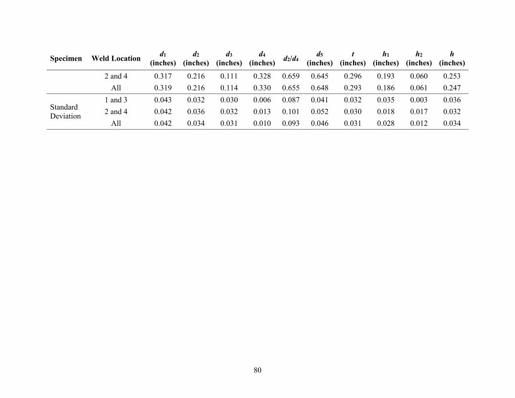
80


d2 (inches)

d3 (inches)


(inches) t

(inches) h1

(inches) h2

(inches) h

(inches)

2 and 4 0.317 0.216 0.111 0.328 0.659 0.645 0.296 0.193 0.060 0.253 All 0.319 0.216 0.114 0.330 0.655 0.648 0.293 0.186 0.061 0.247

Standard Deviation

1 and 3 0.043 0.032 0.030 0.006 0.087 0.041 0.032 0.035 0.003 0.036 2 and 4 0.042 0.036 0.032 0.013 0.101 0.052 0.030 0.018 0.017 0.032

All 0.042 0.034 0.031 0.010 0.093 0.046 0.031 0.028 0.012 0.034

81



d2 (inches)

d3 (inches)


(inches) t

(inches) h1

(inches) h2

(inches) h

(inches)

SA6-1

1 0.227 0.261 0.091 0.353 0.741 0.579 0.320 0.185 0.065 0.250 2 0.256 0.229 0.098 0.328 0.700 0.584 0.310 0.199 0.068 0.267 3 0.253 0.241 0.096 0.337 0.716 0.590 0.313 0.232 0.061 0.293 4 0.226 0.240 0.095 0.336 0.716 0.561 0.310 0.223 0.069 0.292


SA6-2

1 0.235 0.236 0.083 0.319 0.740 0.554 0.314 0.226 0.056 0.282 2 0.185 0.253 0.069 0.321 0.786 0.506 0.319 0.220 0.067 0.287 3 0.222 0.222 0.114 0.337 0.660 0.559 0.302 0.220 0.059 0.279 4 0.256 0.225 0.106 0.331 0.680 0.587 0.307 0.211 0.069 0.280


SA6-3

1 0.241 0.229 0.135 0.363 0.630 0.604 0.321 0.240 0.066 0.306 2 0.245 0.260 0.077 0.337 0.771 0.582 0.320 0.206 0.059 0.265 3 0.220 0.242 0.107 0.349 0.694 0.569 0.305 0.199 0.077 0.275 4 0.219 0.249 0.081 0.329 0.755 0.549 0.315 0.193 0.058 0.252


SA6-4

1 0.229 0.224 0.102 0.326 0.686 0.554 0.302 0.254 0.057 0.312 2 0.247 0.227 0.094 0.321 0.708 0.568 0.284 0.157 0.067 0.223 3 0.223 0.238 0.084 0.321 0.740 0.545 0.315 0.230 0.057 0.286 4 0.171 0.257 0.059 0.315 0.814 0.486 0.311 0.172 0.064 0.237

82


d2 (inches)

d3 (inches)


(inches) t

(inches) h1

(inches) h2

(inches) h

(inches)


SA6-5

1 0.279 0.202 0.123 0.325 0.621 0.605 0.280 0.219 0.064 0.284 2 0.416 0.021 0.297 0.318 0.065 0.734 0.185 0.430 0.051 0.480 3 0.236 0.224 0.102 0.326 0.687 0.562 0.306 0.219 0.066 0.285 4 0.222 0.205 0.121 0.326 0.628 0.548 0.274 0.184 0.056 0.240


SA6-6

1 0.243 0.230 0.093 0.323 0.713 0.566 0.303 0.205 0.056 0.262 2 0.236 0.249 0.070 0.319 0.780 0.555 0.309 0.246 0.066 0.312 3 0.231 0.241 0.088 0.329 0.733 0.560 0.316 0.246 0.057 0.303 4 0.235 0.223 0.098 0.321 0.696 0.556 0.297 0.202 0.066 0.268


SA6-7

1 0.231 0.228 0.092 0.320 0.712 0.552 0.301 0.230 0.055 0.285 2 0.251 0.232 0.090 0.322 0.721 0.572 0.314 0.228 0.065 0.293 3 0.206 0.217 0.105 0.321 0.674 0.527 0.296 0.216 0.055 0.270 4 0.268 0.214 0.105 0.319 0.671 0.587 0.307 0.221 0.062 0.283


SA6-8 1 0.219 0.250 0.167 0.417 0.600 0.636 0.324 0.227 0.056 0.283 2 0.297 0.175 0.152 0.327 0.535 0.624 0.250 0.256 0.067 0.325 3 0.196 0.233 0.103 0.335 0.694 0.532 0.296 0.209 0.059 0.268

83


d2 (inches)

d3 (inches)


(inches) t

(inches) h1

(inches) h2

(inches) h

(inches)


Average 1 and 3 0.231 0.232 0.105 0.338 0.690 0.568 0.307 0.222 0.060 0.283 2 and 4 0.246 0.218 0.110 0.327 0.665 0.574 0.294 0.225 0.064 0.289

All 0.239 0.225 0.107 0.332 0.677 0.571 0.300 0.224 0.062 0.286

Standard Deviation

1 and 3 0.019 0.014 0.022 0.025 0.044 0.028 0.012 0.018 0.006 0.016 2 and 4 0.054 0.057 0.056 0.013 0.175 0.054 0.035 0.061 0.005 0.059

All 0.041 0.041 0.042 0.020 0.126 0.042 0.026 0.044 0.006 0.042

84



d2 (inches)

d3 (inches)


(inches) t

(inches) h1

(inches) h2

(inches) h

(inches)

SA4-1

1 0.248 0.199 0.170 0.369 0.540 0.617 0.290 0.224 0.056 0.280 2 0.152 0.333 0.000 0.333 1.000 0.485 0.374 0.226 0.065 0.292 3 0.253 0.209 0.125 0.335 0.626 0.587 0.285 0.242 0.057 0.299 4 0.266 0.236 0.138 0.374 0.630 0.640 0.304 0.211 0.062 0.273


SA4-2

1 0.258 0.195 0.133 0.328 0.593 0.586 0.282 0.223 0.058 0.280 2 0.219 0.333 0.000 0.333 1.000 0.552 0.358 0.150 0.067 0.218 3 0.253 0.219 0.114 0.333 0.658 0.585 0.301 0.238 0.060 0.298 4 0.191 0.290 0.058 0.348 0.834 0.539 0.316 0.130 0.073 0.203


SA4-3

1 0.226 0.190 0.185 0.375 0.506 0.601 0.281 0.234 0.057 0.292 2 0.196 0.320 0.000 0.320 1.000 0.516 0.372 0.272 0.059 0.331 3 0.244 0.207 0.120 0.326 0.634 0.570 0.286 0.221 0.056 0.277 4 0.182 0.323 0.000 0.323 1.000 0.505 0.377 0.426 0.061 0.487


SA4-4

1 0.255 0.200 0.142 0.342 0.586 0.597 0.290 0.256 0.058 0.314 2 0.210 0.276 0.050 0.326 0.846 0.536 0.323 0.207 0.064 0.271 3 0.277 0.193 0.127 0.321 0.603 0.598 0.297 0.255 0.056 0.312 4 0.197 0.200 0.123 0.323 0.618 0.520 0.256 0.193 0.064 0.257

85


d2 (inches)

d3 (inches)


(inches) t

(inches) h1

(inches) h2

(inches) h

(inches)


SA4-5

1 0.256 0.194 0.127 0.321 0.605 0.576 0.284 0.193 0.055 0.248 2 0.234 0.284 0.053 0.336 0.844 0.571 0.306 0.191 0.067 0.189 3 0.222 0.213 0.125 0.339 0.630 0.560 0.281 0.171 0.063 0.234 4 0.205 0.284 0.075 0.359 0.792 0.564 0.349 0.302 0.061 0.363


SA4-6

1 0.261 0.200 0.135 0.334 0.597 0.596 0.290 0.230 0.058 0.288 2 0.202 0.221 0.102 0.323 0.684 0.525 0.267 0.186 0.064 0.250 3 0.265 0.185 0.141 0.326 0.568 0.591 0.282 0.241 0.059 0.300 4 0.251 0.177 0.150 0.327 0.542 0.578 0.238 0.166 0.064 0.230


SA4-7

1 0.278 0.143 0.180 0.324 0.443 0.601 0.251 0.213 0.052 0.265 2 0.362 0.085 0.246 0.331 0.255 0.693 0.222 0.187 0.067 0.254 3 0.242 0.196 0.129 0.324 0.604 0.567 0.286 0.237 0.054 0.291 4 0.211 0.256 0.081 0.337 0.759 0.548 0.296 0.176 0.068 0.244


SA4-8 1 0.245 0.231 0.115 0.346 0.667 0.591 0.304 0.229 0.063 0.291 2 0.278 0.153 0.181 0.334 0.459 0.612 0.253 0.229 0.058 0.287 3 0.271 0.210 0.111 0.320 0.655 0.591 0.280 0.178 0.065 0.244

86


d2 (inches)

d3 (inches)


(inches) t

(inches) h1

(inches) h2

(inches) h

(inches)


Average 1 and 3 0.253 0.199 0.136 0.335 0.595 0.588 0.286 0.224 0.058 0.282 2 and 4 0.226 0.249 0.086 0.335 0.745 0.560 0.307 0.216 0.064 0.276

All 0.239 0.224 0.111 0.335 0.670 0.574 0.296 0.220 0.061 0.279

Standard Deviation

1 and 3 0.016 0.019 0.023 0.016 0.059 0.015 0.012 0.025 0.004 0.024 2 and 4 0.049 0.071 0.072 0.014 0.215 0.053 0.050 0.070 0.004 0.071

All 0.038 0.057 0.058 0.015 0.173 0.041 0.037 0.052 0.005 0.052

87



d2 (inches)

d3 (inches)


(inches) t

(inches) h1

(inches) h2

(inches) h

(inches)

SA2-1

1 0.196 0.289 0.035 0.324 0.891 0.520 0.332 0.179 0.063 0.242 2 0.200 0.210 0.116 0.326 0.643 0.526 0.289 0.217 0.065 0.282 3 0.188 0.255 0.076 0.331 0.771 0.519 0.311 0.232 0.066 0.298 4 0.197 0.206 0.120 0.326 0.632 0.523 0.292 0.223 0.063 0.287


SA2-2

1 0.196 0.217 0.114 0.332 0.654 0.527 0.294 0.204 0.066 0.270 2 0.173 0.279 0.053 0.332 0.840 0.505 0.330 0.325 0.064 0.389 3 0.205 0.224 0.105 0.329 0.681 0.535 0.296 0.206 0.067 0.273 4 0.264 0.202 0.147 0.349 0.580 0.613 0.320 0.475 0.068 0.543


SA2-3

1 0.194 0.269 0.061 0.330 0.814 0.524 0.317 0.190 0.064 0.253 2 0.182 0.210 0.120 0.331 0.636 0.513 0.283 0.216 0.066 0.282 3 0.167 0.208 0.131 0.339 0.614 0.506 0.297 0.280 0.069 0.349 4 0.202 0.206 0.118 0.324 0.636 0.526 0.302 0.269 0.063 0.332


SA2-4

1 0.212 0.208 0.116 0.323 0.643 0.535 0.287 0.237 0.064 0.301 2 0.333 0.194 0.125 0.319 0.609 0.652 0.340 0.443 0.058 0.501 3 0.188 0.221 0.114 0.334 0.661 0.522 0.288 0.205 0.068 0.274 4 0.182 0.242 0.082 0.324 0.747 0.506 0.292 0.212 0.060 0.273

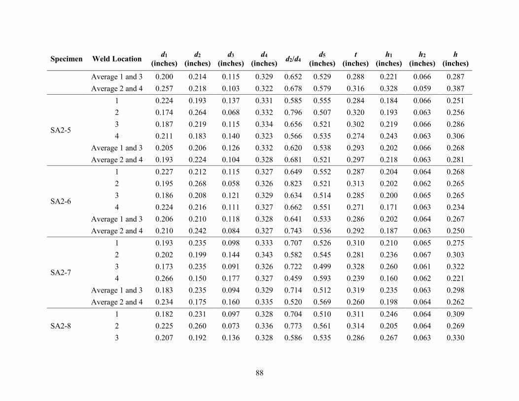
88


d2 (inches)

d3 (inches)


(inches) t

(inches) h1

(inches) h2

(inches) h

(inches)


SA2-5

1 0.224 0.193 0.137 0.331 0.585 0.555 0.284 0.184 0.066 0.251 2 0.174 0.264 0.068 0.332 0.796 0.507 0.320 0.193 0.063 0.256 3 0.187 0.219 0.115 0.334 0.656 0.521 0.302 0.219 0.066 0.286 4 0.211 0.183 0.140 0.323 0.566 0.535 0.274 0.243 0.063 0.306


SA2-6

1 0.227 0.212 0.115 0.327 0.649 0.552 0.287 0.204 0.064 0.268 2 0.195 0.268 0.058 0.326 0.823 0.521 0.313 0.202 0.062 0.265 3 0.186 0.208 0.121 0.329 0.634 0.514 0.285 0.200 0.065 0.265 4 0.224 0.216 0.111 0.327 0.662 0.551 0.271 0.171 0.063 0.234


SA2-7

1 0.193 0.235 0.098 0.333 0.707 0.526 0.310 0.210 0.065 0.275 2 0.202 0.199 0.144 0.343 0.582 0.545 0.281 0.236 0.067 0.303 3 0.173 0.235 0.091 0.326 0.722 0.499 0.328 0.260 0.061 0.322 4 0.266 0.150 0.177 0.327 0.459 0.593 0.239 0.160 0.062 0.221


SA2-8 1 0.182 0.231 0.097 0.328 0.704 0.510 0.311 0.246 0.064 0.309 2 0.225 0.260 0.073 0.336 0.773 0.561 0.314 0.205 0.064 0.269 3 0.207 0.192 0.136 0.328 0.586 0.535 0.286 0.267 0.063 0.330

89


d2 (inches)

d3 (inches)


(inches) t

(inches) h1

(inches) h2

(inches) h

(inches)


Average 1 and 3 0.195 0.226 0.104 0.330 0.686 0.525 0.301 0.220 0.065 0.285 2 and 4 0.224 0.223 0.106 0.329 0.678 0.554 0.302 0.253 0.063 0.316

All 0.210 0.225 0.105 0.330 0.682 0.539 0.301 0.237 0.064 0.301

Standard Deviation

1 and 3 0.017 0.026 0.027 0.004 0.082 0.015 0.016 0.030 0.002 0.030 2 and 4 0.054 0.038 0.039 0.008 0.116 0.054 0.031 0.090 0.003 0.090

All 0.042 0.032 0.033 0.006 0.099 0.042 0.024 0.068 0.003 0.068

90

Table 27. Weld dimensions of FIL series.


d2 (inches)

d3 (inches)


(inches) t

(inches) h1

(inches) h2

(inches) h

(inches)

FIL-1

1 0.241 0.248 0.076 0.324 0.767 0.565 0.353 0.290 0.067 0.356 2 0.259 0.226 0.108 0.335 0.675 0.594 0.312 0.230 0.063 0.293 3 0.278 0.184 0.148 0.332 0.555 0.610 0.293 0.310 0.070 0.380 4 0.248 0.218 0.097 0.315 0.691 0.563 0.319 0.316 0.056 0.372


FIL-2

1 0.269 0.172 0.154 0.326 0.528 0.594 0.300 0.334 0.060 0.334 2 0.262 0.202 0.130 0.332 0.608 0.594 0.314 0.298 0.069 0.366 3 0.263 0.218 0.122 0.340 0.642 0.602 0.318 0.378 0.068 0.445 4 0.240 0.222 0.099 0.321 0.690 0.561 0.310 0.256 0.065 0.321


FIL-3

1 0.267 0.206 0.119 0.324 0.634 0.591 0.316 0.333 0.060 0.393 2 0.205 0.272 0.044 0.316 0.860 0.521 0.357 0.328 0.065 0.392 3 0.255 0.216 0.116 0.332 0.650 0.587 0.316 0.328 0.060 0.388 4 0.268 0.150 0.181 0.331 0.453 0.599 0.301 0.292 0.070 0.362


FIL-4

1 0.261 0.225 0.105 0.329 0.682 0.591 0.335 0.336 0.060 0.396 2 0.241 0.211 0.116 0.327 0.646 0.568 0.320 0.301 0.067 0.368 3 0.235 0.213 0.110 0.323 0.661 0.558 0.327 0.355 0.061 0.416 4 0.264 0.334 0.000 0.334 1.000 0.598 0.293 0.246 0.070 0.317

91


d2 (inches)

d3 (inches)


(inches) t

(inches) h1

(inches) h2

(inches) h

(inches)


FIL-5

1 0.269 0.233 0.092 0.325 0.718 0.594 0.328 0.298 0.067 0.365 2 0.284 0.151 0.165 0.315 0.478 0.600 0.273 0.256 0.054 0.311 3 0.301 0.175 0.151 0.326 0.538 0.631 0.310 0.317 0.066 0.384 4 0.275 0.180 0.137 0.316 0.569 0.591 0.289 0.275 0.057 0.331


FIL-6

1 0.270 0.208 0.117 0.326 0.640 0.596 0.314 0.304 0.060 0.364 2 0.196 0.265 0.058 0.323 0.821 0.519 0.353 0.286 0.066 0.353 3 0.285 0.215 0.109 0.325 0.663 0.610 0.319 0.331 0.061 0.392 4 0.271 0.164 0.160 0.324 0.507 0.595 0.289 0.267 0.065 0.332


FIL-7

1 0.324 0.079 0.253 0.332 0.239 0.657 0.235 0.252 0.067 0.318 2 0.326 0.082 0.249 0.331 0.249 0.658 0.244 0.255 0.060 0.315 3 0.265 0.221 0.100 0.321 0.689 0.585 0.304 0.245 0.065 0.310 4 0.286 0.206 0.120 0.326 0.633 0.612 0.300 0.242 0.059 0.301


FIL-8 1 0.232 0.232 0.091 0.323 0.720 0.555 0.345 0.253 0.065 0.318 2 0.245 0.194 0.135 0.328 0.589 0.573 0.311 0.278 0.059 0.337 3 0.246 0.220 0.107 0.327 0.672 0.574 0.292 0.265 0.066 0.330

92


d2 (inches)

d3 (inches)


(inches) t

(inches) h1

(inches) h2

(inches) h

(inches)


Average 1 and 3 0.266 0.204 0.123 0.327 0.625 0.594 0.313 0.308 0.064 0.368 2 and 4 0.260 0.202 0.122 0.325 0.624 0.584 0.303 0.274 0.062 0.336

All 0.263 0.203 0.123 0.326 0.624 0.589 0.308 0.291 0.063 0.352

Standard Deviation

1 and 3 0.024 0.039 0.041 0.005 0.122 0.026 0.027 0.039 0.004 0.038 2 and 4 0.032 0.058 0.058 0.007 0.177 0.034 0.029 0.028 0.005 0.029

All 0.028 0.049 0.049 0.006 0.150 0.030 0.028 0.037 0.005 0.037

93

Table 28. Weld dimensions of OB series.


d2 (inches)

d3 (inches)


(inches) t

(inches) h1

(inches) h2

(inches) h

(inches)

OB-1

1 0.448 0.094 0.234 0.328 0.288 0.776 0.262 0.254 0.074 0.328 2 0.213 0.241 0.088 0.329 0.732 0.542 0.342 0.255 0.085 0.341 3 0.364 0.204 0.127 0.331 0.616 0.695 0.314 0.265 0.075 0.341 4 0.238 0.215 0.126 0.341 0.630 0.579 0.312 0.200 0.090 0.290


OB-2

1 0.361 0.220 0.117 0.337 0.652 0.697 0.329 0.246 0.076 0.321 2 0.264 0.240 0.088 0.329 0.731 0.593 0.337 0.224 0.087 0.311 3 0.345 0.199 0.130 0.329 0.604 0.067 0.325 0.277 0.074 0.351 4 0.267 0.200 0.129 0.329 0.609 0.596 0.320 0.225 0.086 0.311


OB-3

1 0.356 0.228 0.120 0.348 0.656 0.704 0.322 0.195 0.074 0.269 2 0.285 0.242 0.071 0.313 0.774 0.598 0.348 0.241 0.061 0.302 3 0.332 0.224 0.103 0.327 0.684 0.661 0.319 0.212 0.069 0.281 4 0.310 0.199 0.108 0.307 0.647 0.617 0.314 0.227 0.061 0.287


OB-4

1 0.306 0.304 0.015 0.319 0.954 0.625 0.356 0.192 0.062 0.254 2 0.307 0.226 0.100 0.327 0.691 0.634 0.324 0.238 0.082 0.320 3 0.349 0.209 0.109 0.318 0.657 0.668 0.328 0.255 0.061 0.316 4 0.253 0.240 0.114 0.354 0.677 0.636 0.326 0.235 0.095 0.330

94


d2 (inches)

d3 (inches)


(inches) t

(inches) h1

(inches) h2

(inches) h

(inches)


OB-5

1 0.296 0.222 0.116 0.337 0.659 0.633 0.320 0.224 0.092 0.316 2 0.338 0.220 0.121 0.341 0.646 0.679 0.323 0.241 0.078 0.319 3 0.290 0.222 0.109 0.332 0.670 0.622 0.324 0.214 0.089 0.303 4 0.332 0.204 0.131 0.335 0.610 0.667 0.313 0.250 0.079 0.329


OB-6

1 0.305 0.221 0.108 0.330 0.672 0.634 0.305 0.210 0.089 0.299 2 0.326 0.203 0.133 0.336 0.605 0.662 0.307 0.230 0.076 0.306 3 0.288 0.228 0.120 0.348 0.655 0.636 0.327 0.225 0.095 0.320 4 0.351 0.185 0.161 0.345 0.535 0.696 0.306 0.249 0.077 0.327


OB-7

1 0.339 0.202 0.142 0.344 0.587 0.683 0.307 0.226 0.077 0.303 2 0.293 0.225 0.103 0.328 0.685 0.621 0.310 0.194 0.087 0.281 3 0.328 0.243 0.088 0.331 0.733 0.659 0.341 0.236 0.072 0.308 4 0.310 0.271 0.074 0.345 0.785 0.655 0.338 0.195 0.090 0.285


OB-8 1 0.332 0.235 0.097 0.332 0.708 0.664 0.333 0.229 0.074 0.303 2 0.313 0.207 0.125 0.332 0.624 0.645 0.299 0.190 0.086 0.276 3 0.366 0.230 0.101 0.332 0.694 0.698 0.329 0.261 0.073 0.333

95


d2 (inches)

d3 (inches)


(inches) t

(inches) h1

(inches) h2

(inches) h

(inches)


OB-9

1 0.338 0.252 0.066 0.319 0.792 0.656 0.328 0.202 0.062 0.264 2 0.311 0.205 0.127 0.332 0.618 0.644 0.345 0.228 0.062 0.320 3 0.371 0.233 0.085 0.318 0.733 0.689 0.329 0.238 0.059 0.297 4 0.327 0.174 0.146 0.320 0.545 0.647 0.282 0.244 0.063 0.307


OB-10

1 0.339 0.176 0.166 0.341 0.515 0.680 0.278 0.220 0.083 0.303 2 0.309 0.242 0.072 0.314 0.772 0.622 0.346 0.246 0.072 0.317 3 0.329 0.178 0.151 0.329 0.541 0.657 0.293 0.218 0.084 0.302 4 0.308 0.241 0.096 0.337 0.715 0.645 0.340 0.238 0.079 0.317


OB-11

1 0.350 0.149 0.193 0.342 0.436 0.692 0.279 0.228 0.083 0.310 2 0.290 0.176 0.147 0.323 0.546 0.613 0.295 0.221 0.077 0.298 3 0.345 0.215 0.116 0.331 0.649 0.675 0.313 0.235 0.083 0.318 4 0.299 0.220 0.112 0.332 0.664 0.630 0.326 0.236 0.079 0.314


OB-12 1 0.341 0.233 0.121 0.355 0.658 0.696 0.321 0.198 0.089 0.286 2 0.339 0.200 0.131 0.331 0.604 0.671 0.309 0.233 0.078 0.311

96


d2 (inches)

d3 (inches)


(inches) t

(inches) h1

(inches) h2

(inches) h

(inches)

3 0.354 0.219 0.114 0.333 0.659 0.686 0.319 0.214 0.084 0.298 4 0.323 0.231 0.098 0.329 0.701 0.652 0.325 0.225 0.077 0.302


OB-13

1 0.345 0.242 0.095 0.336 0.719 0.681 0.323 0.211 0.090 0.301 2 0.327 0.202 0.127 0.329 0.614 0.656 0.301 0.217 0.076 0.292 3 0.331 0.211 0.121 0.332 0.635 0.663 0.310 0.218 0.088 0.306 4 0.346 0.141 0.200 0.342 0.413 0.688 0.279 0.216 0.082 0.298


OB-14

1 0.339 0.167 0.166 0.333 0.501 0.672 0.300 0.228 0.077 0.305 2 0.339 0.188 0.143 0.331 0.568 0.670 0.299 0.204 0.087 0.290 3 0.290 0.216 0.121 0.337 0.641 0.626 0.332 0.229 0.079 0.307 4 0.335 0.201 0.137 0.338 0.595 0.673 0.308 0.228 0.087 0.314


OB-15

1 0.257 0.213 0.129 0.342 0.624 0.599 0.315 0.242 0.075 0.317 2 0.325 0.192 0.134 0.327 0.588 0.651 0.297 0.223 0.085 0.308 3 0.253 0.223 0.109 0.332 0.672 0.585 0.307 0.307 0.078 0.385 4 0.318 0.222 0.108 0.330 0.674 0.648 0.315 0.230 0.087 0.317


OB-16 1 0.376 0.172 0.160 0.332 0.517 0.708 0.291 0.220 0.082 0.302

97


d2 (inches)

d3 (inches)


(inches) t

(inches) h1

(inches) h2

(inches) h

(inches)

2 0.213 0.216 0.109 0.326 0.665 0.539 0.353 0.279 0.073 0.351 3 0.391 0.171 0.160 0.331 0.516 0.722 0.336 0.295 0.084 0.379 4 0.248 0.212 0.118 0.329 0.643 0.577 0.319 0.220 0.075 0.295


Average 1 and 3 0.336 0.211 0.122 0.333 0.636 0.650 0.316 0.232 0.078 0.310 2 and 4 0.303 0.212 0.119 0.331 0.641 0.635 0.318 0.229 0.079 0.309

All 0.319 0.212 0.120 0.332 0.639 0.643 0.317 0.230 0.079 0.309

Standard Deviation

1 and 3 0.035 0.029 0.031 0.007 0.092 0.079 0.015 0.021 0.009 0.022 2 and 4 0.036 0.020 0.022 0.008 0.063 0.038 0.014 0.014 0.009 0.012

All 0.039 0.024 0.027 0.007 0.078 0.062 0.014 0.018 0.009 0.017

98

Table 29. Weld dimensions of UB series.


d2 (inches)

d3 (inches)


(inches) t

(inches) h1

(inches) h2

(inches) h

(inches)

UB-1

1 0.251 0.223 0.113 0.335 0.664 0.587 0.332 0.235 0.087 0.322 2 0.345 0.166 0.166 0.333 0.500 0.678 0.280 0.218 0.083 0.301 3 0.262 0.211 0.120 0.331 0.637 0.593 0.318 0.230 0.082 0.312 4 0.347 0.203 0.129 0.332 0.612 0.679 0.303 0.218 0.079 0.294


UB-2

1 0.322 0.183 0.151 0.334 0.549 0.656 0.293 0.267 0.078 0.345 2 0.261 0.224 0.110 0.334 0.669 0.595 0.327 0.282 0.083 0.371 3 0.311 0.241 0.094 0.334 0.720 0.645 0.321 0.215 0.083 0.298 4 0.270 0.250 0.086 0.336 0.744 0.606 0.336 0.223 0.080 0.302


UB-3

1 0.281 0.226 0.080 0.306 0.740 0.587 0.344 0.263 0.063 0.326 2 0.367 0.177 0.157 0.334 0.529 0.701 0.286 0.216 0.081 0.296 3 0.280 0.172 0.134 0.306 0.563 0.586 0.307 0.248 0.063 0.311 4 0.337 0.148 0.183 0.332 0.447 0.669 0.275 0.240 0.078 0.318


UB-4

1 0.254 0.214 0.117 0.331 0.647 0.585 0.323 0.231 0.082 0.313 2 0.344 0.144 0.169 0.312 0.459 0.656 0.276 0.234 0.077 0.311 3 0.206 0.189 0.144 0.333 0.567 0.539 0.363 0.286 0.081 0.366 4 0.370 0.156 0.176 0.332 0.469 0.702 0.285 0.232 0.083 0.315

99


d2 (inches)

d3 (inches)


(inches) t

(inches) h1

(inches) h2

(inches) h

(inches)


UB-5

1 0.279 0.240 0.103 0.343 0.699 0.622 0.337 0.230 0.085 0.315 2 0.333 0.137 0.192 0.329 0.417 0.662 0.264 0.207 0.083 0.290 3 0.258 0.204 0.129 0.333 0.613 0.591 0.328 0.229 0.084 0.313 4 0.329 0.202 0.129 0.331 0.609 0.660 0.297 0.220 0.080 0.300


UB-6

1 0.262 0.251 0.089 0.342 0.732 0.604 0.346 0.304 0.088 0.392 2 0.356 0.175 0.154 0.330 0.532 0.686 0.283 0.214 0.082 0.296 3 0.287 0.201 0.138 0.340 0.593 0.626 0.309 0.209 0.083 0.293 4 0.337 0.193 0.140 0.333 0.580 0.670 0.298 0.222 0.081 0.303


UB-7

1 0.265 0.241 0.094 0.335 0.719 0.600 0.337 0.315 0.085 0.400 2 0.327 0.191 0.142 0.333 0.573 0.660 0.287 0.205 0.086 0.291 3 0.245 0.247 0.087 0.334 0.739 0.580 0.349 0.329 0.085 0.414 4 0.321 0.179 0.152 0.331 0.541 0.653 0.287 0.225 0.080 0.304


UB-8 1 0.247 0.224 0.115 0.338 0.661 0.585 0.342 0.277 0.082 0.359 2 0.326 0.191 0.140 0.331 0.577 0.657 0.286 0.258 0.083 0.343 3 0.248 0.254 0.083 0.338 0.753 0.586 0.345 0.321 0.084 0.404

100


d2 (inches)

d3 (inches)


(inches) t

(inches) h1

(inches) h2

(inches) h

(inches)


UB-9

1 0.280 0.249 0.084 0.333 0.747 0.613 0.341 0.316 0.079 0.394 2 0.281 0.205 0.119 0.324 0.633 0.603 0.314 0.288 0.084 0.372 3 0.251 0.259 0.072 0.331 0.782 0.058 0.366 0.303 0.080 0.383 4 0.305 0.198 0.137 0.335 0.590 0.640 0.296 0.219 0.083 0.302


UB-10

1 0.273 0.244 0.088 0.332 0.734 0.605 0.332 0.285 0.084 0.370 2 0.274 0.227 0.103 0.329 0.688 0.604 0.322 0.231 0.078 0.309 3 0.262 0.221 0.113 0.334 0.662 0.595 0.317 0.228 0.086 0.315 4 0.308 0.225 0.108 0.333 0.677 0.641 0.349 0.280 0.074 0.354


UB-11

1 0.298 0.187 0.141 0.328 0.571 0.626 0.298 0.243 0.072 0.315 2 0.276 0.211 0.126 0.337 0.626 0.613 0.311 0.225 0.087 0.312 3 0.348 0.175 0.161 0.336 0.521 0.684 0.327 0.231 0.077 0.307 4 0.270 0.203 0.128 0.331 0.614 0.602 0.311 0.239 0.083 0.322


UB-12 1 0.340 0.176 0.160 0.336 0.523 0.676 0.302 0.271 0.074 0.345 2 0.295 0.193 0.140 0.333 0.581 0.628 0.292 0.205 0.085 0.290

101


d2 (inches)

d3 (inches)


(inches) t

(inches) h1

(inches) h2

(inches) h

(inches)

3 0.291 0.192 0.154 0.346 0.556 0.637 0.297 0.206 0.081 0.286 4 0.263 0.157 0.169 0.326 0.482 0.589 0.283 0.225 0.082 0.307


UB-13

1 0.343 0.148 0.186 0.334 0.444 0.677 0.270 0.212 0.070 0.282 2 0.300 0.228 0.107 0.335 0.679 0.635 0.326 0.234 0.085 0.319 3 0.361 0.157 0.181 0.338 0.465 0.699 0.264 0.237 0.073 0.310 4 0.311 0.205 0.126 0.331 0.620 0.642 0.300 0.214 0.083 0.296


UB-14

1 0.307 0.218 0.120 0.338 0.644 0.645 0.306 0.222 0.094 0.315 2 0.342 0.215 0.122 0.336 0.638 0.678 0.304 0.207 0.078 0.285 3 0.282 0.216 0.120 0.336 0.643 0.618 0.315 0.233 0.086 0.319 4 0.342 0.187 0.143 0.330 0.567 0.672 0.292 0.225 0.077 0.302


UB-15

1 0.318 0.243 0.089 0.333 0.731 0.650 0.339 0.267 0.076 0.343 2 0.275 0.198 0.146 0.344 0.577 0.619 0.316 0.227 0.087 0.314 3 0.343 0.187 0.143 0.330 0.567 0.673 0.290 0.213 0.077 0.290 4 0.295 0.204 0.132 0.336 0.607 0.631 0.310 0.243 0.081 0.324


UB-16 1 0.268 0.188 0.148 0.336 0.559 0.604 0.315 0.252 0.083 0.335

102


d2 (inches)

d3 (inches)


(inches) t

(inches) h1

(inches) h2

(inches) h

(inches)

2 0.311 0.165 0.176 0.341 0.485 0.652 0.299 0.220 0.080 0.300 3 0.254 0.199 0.139 0.339 0.588 0.593 0.298 0.310 0.083 0.393 4 0.420 0.168 0.176 0.344 0.489 0.764 0.316 0.295 0.082 0.377


Average 1 and 3 0.284 0.212 0.122 0.334 0.639 0.601 0.321 0.257 0.080 0.337 2 and 4 0.317 0.191 0.141 0.333 0.575 0.649 0.300 0.233 0.082 0.315

All 0.300 0.202 0.131 0.333 0.607 0.625 0.311 0.245 0.081 0.326

Standard Deviation

1 and 3 0.034 0.026 0.027 0.008 0.079 0.079 0.021 0.030 0.007 0.032 2 and 4 0.033 0.024 0.023 0.004 0.070 0.033 0.017 0.018 0.003 0.019

All 0.037 0.027 0.026 0.006 0.080 0.064 0.022 0.027 0.005 0.028

103

Table 30. Weld dimensions of W series.


d2 (inches)

d3 (inches)


(inches) t

(inches) h

(inches)

W-1

1 0.432 0.092 0.232 0.325 0.283 0.757 0.220 0.319 2 0.318 0.122 0.197 0.319 0.382 0.637 0.304 0.382 3 0.401 0.106 0.219 0.324 0.327 0.725 0.285 0.382 4 0.394 0.087 0.233 0.320 0.272 0.714 0.298 0.385

Average 1 and 3 0.417 0.099 0.226 0.325 0.305 0.741 0.253 0.351 Average 2 and 4a 0.356 0.105 0.215 0.320 0.327 0.676 0.301 0.384

W-2

1 0.401 0.106 0.219 0.324 0.327 0.725 0.285 0.382 2 0.394 0.087 0.233 0.320 0.272 0.714 0.298 0.385 3 0.348 0.104 0.221 0.325 0.320 0.673 0.248 0.384 4 0.388 0.125 0.197 0.323 0.387 0.711 0.291 0.331

Average 1 and 3a 0.375 0.105 0.220 0.325 0.324 0.699 0.267 0.383 Average 2 and 4 0.391 0.106 0.215 0.322 0.330 0.713 0.295 0.358

W-3

1 0.348 0.104 0.221 0.325 0.320 0.673 0.248 0.384 2 0.388 0.125 0.197 0.323 0.387 0.711 0.291 0.331 3 0.363 0.141 0.200 0.341 0.413 0.704 0.255 0.418 4 0.365 0.141 0.189 0.330 0.427 0.694 0.298 0.323


W-4

1 0.363 0.141 0.200 0.341 0.413 0.704 0.255 0.418 2 0.365 0.141 0.189 0.330 0.427 0.694 0.298 0.323 3 0.351 0.139 0.183 0.322 0.432 0.673 0.222 0.313 4 0.386 0.101 0.205 0.306 0.330 0.692 0.263 0.452

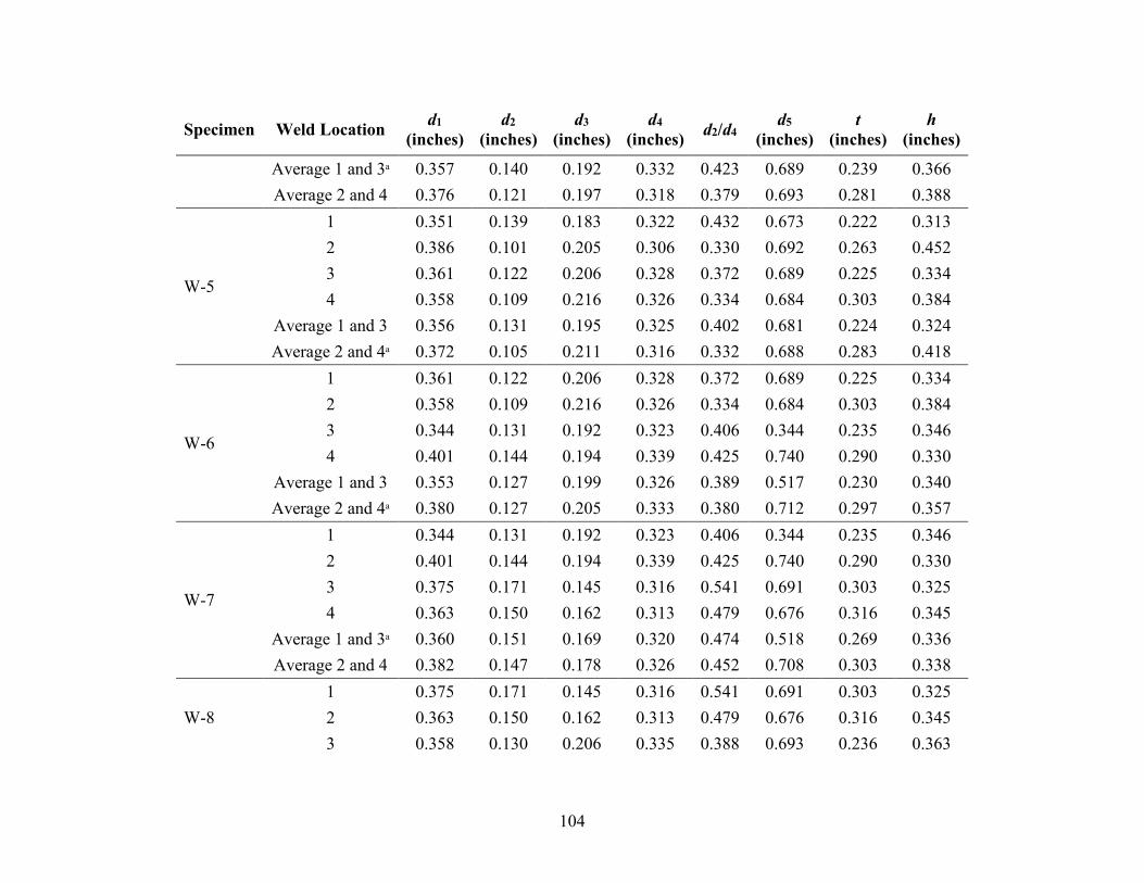
104


d2 (inches)

d3 (inches)


(inches) t

(inches) h

(inches)


W-5

1 0.351 0.139 0.183 0.322 0.432 0.673 0.222 0.313 2 0.386 0.101 0.205 0.306 0.330 0.692 0.263 0.452 3 0.361 0.122 0.206 0.328 0.372 0.689 0.225 0.334 4 0.358 0.109 0.216 0.326 0.334 0.684 0.303 0.384


W-6

1 0.361 0.122 0.206 0.328 0.372 0.689 0.225 0.334 2 0.358 0.109 0.216 0.326 0.334 0.684 0.303 0.384 3 0.344 0.131 0.192 0.323 0.406 0.344 0.235 0.346 4 0.401 0.144 0.194 0.339 0.425 0.740 0.290 0.330


W-7

1 0.344 0.131 0.192 0.323 0.406 0.344 0.235 0.346 2 0.401 0.144 0.194 0.339 0.425 0.740 0.290 0.330 3 0.375 0.171 0.145 0.316 0.541 0.691 0.303 0.325 4 0.363 0.150 0.162 0.313 0.479 0.676 0.316 0.345


W-8 1 0.375 0.171 0.145 0.316 0.541 0.691 0.303 0.325 2 0.363 0.150 0.162 0.313 0.479 0.676 0.316 0.345 3 0.358 0.130 0.206 0.335 0.388 0.693 0.236 0.363

105


d2 (inches)

d3 (inches)


(inches) t

(inches) h

(inches)

4 0.357 0.141 0.186 0.326 0.433 0.683 0.296 0.335 Average 1 and 3 0.367 0.151 0.176 0.326 0.465 0.692 0.270 0.344 Average 2 and 4a 0.360 0.146 0.174 0.320 0.456 0.680 0.306 0.340

W-9

1 0.358 0.130 0.206 0.335 0.388 0.693 0.236 0.363 2 0.357 0.141 0.186 0.326 0.433 0.683 0.296 0.335 3 0.369 0.110 0.210 0.320 0.344 0.690 0.288 0.369 4 0.359 0.137 0.188 0.326 0.420 0.685 0.290 0.339


W-10

1 0.369 0.110 0.210 0.320 0.344 0.690 0.288 0.369 2 0.359 0.137 0.188 0.326 0.420 0.685 0.290 0.339 3 0.344 0.122 0.196 0.318 0.384 0.663 0.279 0.329 4 0.381 0.149 0.192 0.341 0.437 0.721 0.302 0.355


W-11

1 0.344 0.122 0.196 0.318 0.384 0.663 0.279 0.329 2 0.381 0.149 0.192 0.341 0.437 0.721 0.302 0.355 3 0.361 0.130 0.198 0.329 0.395 0.690 0.288 0.342 4 0.379 0.084 0.237 0.322 0.261 0.701 0.280 0.371


W-12 1 0.361 0.130 0.198 0.329 0.395 0.690 0.288 0.342 2 0.379 0.084 0.237 0.322 0.261 0.701 0.280 0.371

106


d2 (inches)

d3 (inches)


(inches) t

(inches) h

(inches)

3 0.381 0.132 0.189 0.322 0.410 0.702 0.298 0.387 4 0.330 0.174 0.150 0.324 0.537 0.654 0.311 0.347


W-13

1 0.381 0.132 0.189 0.322 0.410 0.702 0.298 0.387 2 0.330 0.174 0.150 0.324 0.537 0.654 0.311 0.347 3 0.396 0.096 0.228 0.324 0.296 0.720 0.301 0.386 4 0.361 0.132 0.203 0.336 0.393 0.697 0.312 0.385


W-14

1 0.396 0.096 0.228 0.324 0.296 0.720 0.301 0.386 2 0.361 0.132 0.203 0.336 0.393 0.697 0.312 0.385 3 0.378 0.108 0.217 0.325 0.332 0.704 0.287 0.341 4 0.292 0.119 0.202 0.322 0.370 0.614 0.297 0.376


W-15

1 0.378 0.108 0.217 0.325 0.332 0.704 0.287 0.341 2 0.292 0.119 0.202 0.322 0.370 0.614 0.297 0.376 3 0.362 0.072 0.236 0.307 .235 0.670 0.268 0.355 4 0.357 0.128 0.192 0.320 0.400 0.677 0.280 0.338


W-16 1 0.362 0.072 0.236 0.307 .235 0.670 0.268 0.355

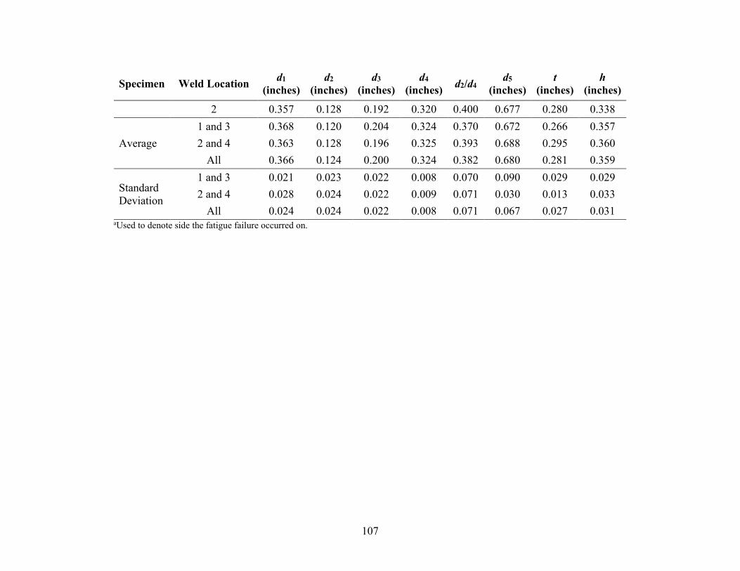
107


d2 (inches)

d3 (inches)


(inches) t

(inches) h

(inches)

2 0.357 0.128 0.192 0.320 0.400 0.677 0.280 0.338

Average 1 and 3 0.368 0.120 0.204 0.324 0.370 0.672 0.266 0.357 2 and 4 0.363 0.128 0.196 0.325 0.393 0.688 0.295 0.360

All 0.366 0.124 0.200 0.324 0.382 0.680 0.281 0.359

Standard Deviation

1 and 3 0.021 0.023 0.022 0.008 0.070 0.090 0.029 0.029 2 and 4 0.028 0.024 0.022 0.009 0.071 0.030 0.013 0.033

All 0.024 0.024 0.022 0.008 0.071 0.067 0.027 0.031 aUsed to denote side the fatigue failure occurred on.

109

APPENDIX C. LASER WELD DIMENSIONS

This appendix presents the data associated with measurements of some of the laser panel specimens. The original intent of etching the welds was to confirm the weld penetration, and, after etching so many laser welded specimens, it was clear that it consistently attained 100 percent or more penetration, and further documentation of weld cross sections ceased. Later in the research program, it was found the dimensions of the weld were relevant to fatigue life; however, only a few of the weld cross sections were photo documented, and the data in this appendix may appear incomplete. Only one face of the laser panel specimens was etched. The weld location syntax used in table 31 is shown in figure 65. Location 1 represents the side with the dominant fatigue crack size because sometimes both welds cracked simultaneously. The remaining column headings in table 31 present the measurements recorded as shown in figure 66.

Because the laser was able to achieve full penetration, there is no definition for the weld throat as there was for the conventional weld processes. To be able to introduce the weld throat dimension in the multiple linear regression statistical analysis, a throat dimension had to be defined for the laser specimens. For this work and for just the laser specimens, the actual throat dimension was taken from the toe of the root reinforcement to the outside of the face weld in a direction aligned with the thickness direction of the rib wall.

Figure 65. Schematic. Denotation of weld locations for laser panel specimens.

110

Figure 66. Schematic. Measured dimensions for laser panel specimens.

Where:

d1 = Weld length along the deck plate. d2 = Weld penetration. d4 = Projected width of rib on deck plate. d2/d4 = Percentage of the weld penetration. t = Actual weld throat measured from the toe of the root reinforcement to the face of the weld aligned in the thickness direction of the rib wall. h = Weld length along the rib plate.

111

Table 31. Weld dimensions of some LP series specimens.


d2 (inches)

d4 (inches) d2/d4 t

(inches) h

(inches)

LP1-1 1 0.109 0.454 0.322 1.410 0.543 0.207 2 0.112 0.392 0.323 1.214 0.450 0.199

LP1-2 1 0.099 0.366 0.322 1.137 0.448 0.206 2 0.120 0.424 0.322 1.317 0.495 0.174

LP1-3 1 0.100 0.377 0.317 1.189 0.450 0.178 2 0.119 0.433 0.323 1.341 0.471 0.164

LP1-4 1 0.142 0.394 0.321 1.227 0.470 0.187 2 0.091 0.419 0.324 1.293 0.485 0.192

LP1-5 1 0.097 0.409 0.317 1.290 0.487 0.192 2 0.110 0.476 0.320 1.488 0.539 0.200

LP1-6 1 0.142 0.432 0.317 1.363 0.515 0.223 2 0.107 0.467 0.317 1.473 0.519 0.215

LP1-7 1 0.106 0.429 0.318 1.349 0.478 0.190 2 0.128 0.432 0.322 1.342 0.494 0.192

LP3-1 1 0.143 0.325 0.325 1.000 0.436 0.195 2 0.138 0.315 0.315 1.000 0.427 0.211

LP3-2 1 0.127 0.382 0.322 1.186 0.481 0.185 2 0.135 0.409 0.320 1.278 0.502 0.198

LP3-6 1 0.160 0.400 0.320 1.250 0.495 0.214 2 0.120 0.404 0.320 1.263 0.497 0.203

113

REFERENCES

1. Sedlacek, G. (1992). “Orthotropic Plate Bridge Decks,” Constructional Steel Design—An International Guide, Chapter 2.10, edited by Dowling, P.J., Harding, J.E., and Björhovde, R., pp. 227–245, Elsevier, Essex, England.

2. Mehue, P. (1981). “Steel Decks in Road Bridges,” International Symposium on the Management of Civil Structures: Surveillance, Maintenance and Repair of Road and Railway Bridges (translated), pp. 609–612, Paris, France.

3. Mehue, P. (1990). “Cracks in Steel Orthotropic Decks,” Proceedings of the International Conference on Bridge Management, pp. 633–642, Surrey, United Kingdom.

4. Mehue, P. (1992). “Repair Procedures for Cracks in Steel Orthotropic Decks,” Proceedings of the 3rd International Workshop on Bridge Rehabilitation, pp. 159–163, Darmstadt, Germany.

5. Burdekin, F.M. (1981). “Fatigue Cracks in Some Steel Bridges,” International Symposium on the Management of Civil Structures: Surveillance, Maintenance and Repair of Road and Railway Bridges (translated), pp. 163–167, Paris, France.

6. Leendertz, J.S. and Jong de, F.B.P. (2003). “Fatigue Aspects of Orthotropic Steel Decks,” Proceedings of the Lightweight Bridge Decks: European Bridge Engineering Conference, pp. 1–13, Rotterdam, The Netherlands.

7. AASHTO. (2007). AASHTO LRFD Bridge Design Specifications, Fourth Edition, American Association of State Highway and Transportation Officials, Washington, DC.

8. AASHTO. (2014). AASHTO LRFD Bridge Design Specifications, Seventh Edition, American Association of State Highway and Transportation Officials, Washington, DC.

9. Hobbacher, A. (2008). Recommendations for Fatigue Design of Welded Joints and Components, IIW Document IIW-1823-07, International Institute of Welding, Paris, France.

10. Connor, R.J. et al. (2012). Manual for Design, Construction, and Maintenance of Orthotropic Steel Deck Bridges, Report No. FHWA-IF-12-027, Federal Highway Administration. Washington, DC.

11. R Core Team. (2014). R: A Language and Environment for Statistical Computing, R Foundation for Statistical Computing, Vienna, Austria, obtained from: http://www. R-project.org, last accessed June 1, 2016.

HRDI-40/02-17(WEB)E

Optimization of Rib-to-Deck Welds for Steel Orthotropic ... · PDF fileOptimization of...

Documents

Transcript of Optimization of Rib-to-Deck Welds for Steel Orthotropic ... · PDF fileOptimization of...