Optimization methods and their applications in DSP · Optimization methods and their applications...
65
Optimization methods and their applications in DSP Ivan Tashev Principal Architect Microsoft Research
Transcript of Optimization methods and their applications in DSP · Optimization methods and their applications...

Optimization methods and their
applications in DSP
Ivan Tashev
Principal Architect
Microsoft Research

Tutorial outline
• Introduction
• Single parameter optimization
• Multidimensional optimization
• Practical aspects and distributed optimization
• Examples
• Conclusions and Q&A
1/12/2012
2
Optimization methods in DSP

1/12/2012
3
Optimization methods in DSP

Mathematical optimization
• Subfields▫ Convex programming
Linear programming
Second order programming
▫ Integer programming▫ Quadratic programming▫ Fractional programming▫ Non-linear programming▫ Multi-objective programming▫ Multi-modal optimization
• Optimization algorithms – typically iterative
1/12/2012Optimization methods in DSP
4
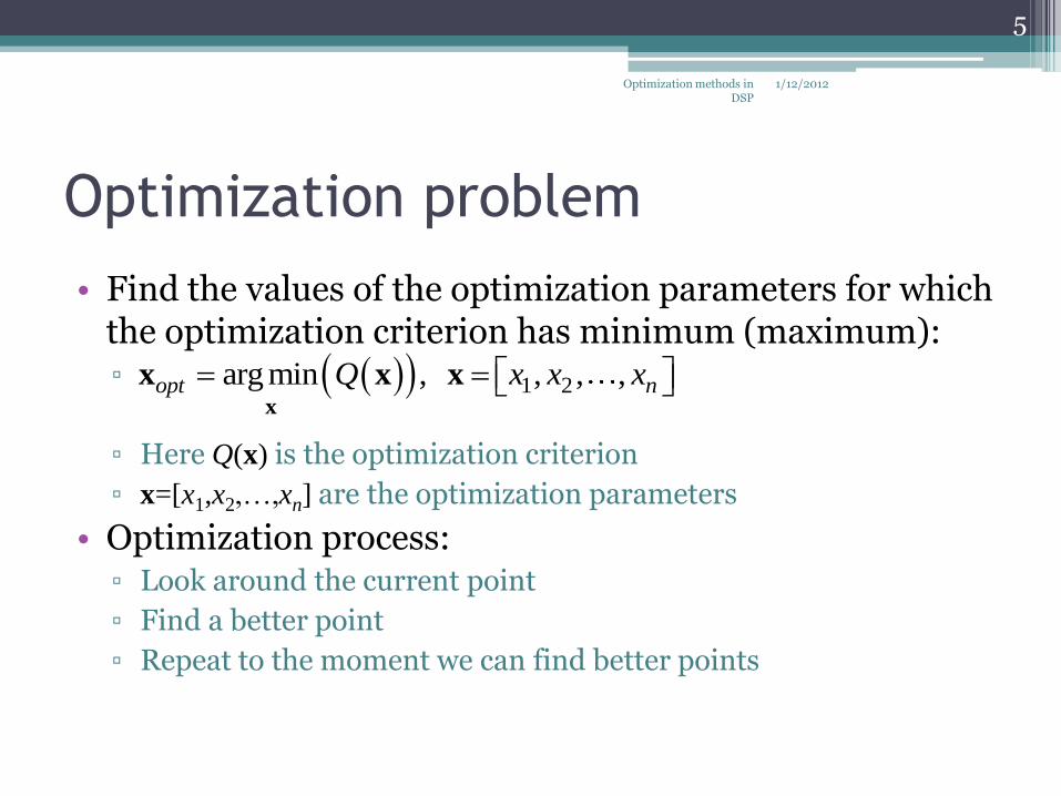
Optimization problem
• Find the values of the optimization parameters for which the optimization criterion has minimum (maximum):▫
▫ Here Q(x) is the optimization criterion
▫ x=[x1,x2,…,xn] are the optimization parameters
• Optimization process:▫ Look around the current point
▫ Find a better point
▫ Repeat to the moment we can find better points
1 2arg min , , , ,opt nQ x x x x
x x x
1/12/2012
5
Optimization methods in DSP

Optimization criteria
• Also called objective or cost function• It is a single number only in very simple cases
▫ In reality we have multiple requirements (sub-criteria)
• Sum:
• Multiplication:
• Minimax:
• Limiting:
• Local and global minimum
1
0
M
i ii
Q w q
1
0
M
ii
Q q
maxi i
Q wq
max ,min ,i i i iq m q
1/12/2012
6
Optimization methods in DSP

Constrained optimization
• Notation:▫
• Constraints convert the optimization problem from mathematical to real
• Parameter values constraints▫
• Intermediate values constraints▫
• Relation constraints▫
i i ia x b
i ic F d x
0G x
1/12/2012
7
Optimization methods in DSP
arg min subject to i i i
opti i
a x bQ
c F d
x
x xx

Introducing the constraints
• Convert the constrained optimization problem into unconstrained
• Punishing functions:▫ Constant: if xi>bi pj =1e10; else pj=0;
▫ Linear: if xi>bi pj =(xi – bi); else pj=0;
▫ Quadratic: if xi>bi pj =(xi – bi)2; else pj=0;
• Adding the punishing function to the optimization criterion:▫ j j
J
Q Q p
1/12/2012
8
Optimization methods in DSP
1/12/2012
9
Optimization methods in DSP

General assumptions
• One minimum in given interval [a, b] – range of uncertainty
• The goal is to reduce the uncertainty interval – process called bracketing
• Can be iterative
• Simple algorithms, predictable performance
1/12/2012
10
Optimization methods in DSP

Scanning
• Compute the criterion in the middle of N equally wide intervals
• Find the minimal point
• The new interval is times smaller
• This can be repeated for another iteration. Then:
▫ Nopt = 3,
a b
x
Q
new interval
2
1f
N
2
1
K
fN
1/12/2012
11
Optimization methods in DSP

Dichotomy
• “cut in two”, bi-section
• Compute the criterion in the middle of the interval in two very close points
• Select the new interval, repeat
▫1
2 2
K
f
a b
x
new interval 1
new interval 2
Q
1/12/2012
12
Optimization methods in DSP
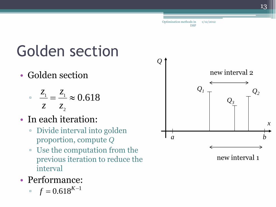
Golden section
• Golden section
▫
• In each iteration:▫ Divide interval into golden
proportion, compute Q
▫ Use the computation from the previous iteration to reduce the interval
• Performance:▫
1/12/2012Optimization methods in DSP
13
1 1
2
0.618z z
z z
10.618Kf
a b
x
new interval 1
new interval 2
Q
Q1
Q3
Q2

Variable step search
• Given start point x0 determine the direction
• Make a step σ towards desired direction
• Increase the step if successful:▫
• Stop when reached worse point
• Repeat from the new point if necessary
1/12/2012Optimization methods in DSP
14
x0
x
Q
1 1, if , 1k k k kQ Q x0+σ x0+2σ x0+4σ x0+8σ
Q1
Q3
Q2
Q4
Q5
α=2.0

Quadratic interpolation
• Also known as Brent’s method:▫ Compute Q in three points
▫ Find a second degree polynomial going trough these three points: Q=c3x
2+c2x+c1
▫ Find the minimum: xopt= – c2/(2c3)
▫ Select the best solution from [Q1,Q2,Q3,Qopt]
• Good for finalizing any of the previous methods
1/12/2012Optimization methods in DSP
15
a b
x
Q
Q1 Q3Q2
Qopt
x1 x2 xopt x3

1/12/2012
16
Optimization methods in DSP

General problem
• Lower chances to have unimodal hypersurface
• Efforts increase exponentially with the number of optimization parameters
• Typically non-deterministic
• Iterative, move from the current work point to a better work point. ▫ Stop when you cant find better work point
• Critical role of the starting point
1/12/2012Optimization methods in DSP
17
Net search
• Multidimensional equivalent of the scanning method
• Compute the criterion in a grid of possible parameter values
• Select the new volume, repeat if necessary
• The only multidimensional method with deterministic performance
• Extremely inefficient, last hope to find a solution
1/12/2012Optimization methods in DSP
18

-2 -1.5 -1 -0.5 0 0.5 1 1.5 2-2
-1.5
-1
-0.5
0
0.5
1
1.5
2
Parameter x1
Pa
ram
ete
r x 2
Function optimization
Simplex method
• Simplex: closed n-dimensional polytopewhich is a convex hull of n+1 vertices
▫ Triangle (2D), tetrahedron (3D), pentachoron (4D), …
• For each iteration:
▫ Compute the criterion in vertices
▫ Find vertex symmetric to the worst
▫ Throw away the worst one
• Stop when the symmetric vortex is even worse
• Variant: variable size simplex
▫ Increase it when you have better point, decrease otherwise: reflection and expansion or reflection and contraction
1/12/2012Optimization methods in DSP
19
12
43

-2 -1.5 -1 -0.5 0 0.5 1 1.5 2-2
-1.5
-1
-0.5
0
0.5
1
1.5
2
Parameter x1
Pa
ram
ete
r x 2
Function optimization
Gaussian optimization
• Fix all parameters, except one, perform single dimensional optimization
• Repeat for the rest of the parameters
• If they are statistically independent – one iteration is sufficient
• Repeat the iteration otherwise
1/12/2012Optimization methods in DSP
20
1
2
3

Gradient methods
• The gradient is a vector pointing towards steepest increase
▫
• For each iteration▫ Compute the gradient
▫ Make a step in the opposite direction, change the work point if successful
▫ Increase the step size if successful, decrease otherwise
▫ Stop when the step is smaller than given value
1/12/2012Optimization methods in DSP
21
-2 -1.5 -1 -0.5 0 0.5 1 1.5 2-2
-1.5
-1
-0.5
0
0.5
1
1.5
2
Parameter x1
Pa
ram
ete
r x 2
Function optimization
0 12
4
3
5
1 2
1 2
n
n
Q Q QQ e e e
x x x

-2 -1.5 -1 -0.5 0 0.5 1 1.5 2-2
-1.5
-1
-0.5
0
0.5
1
1.5
2
Parameter x1
Pa
ram
ete
r x 2
Function optimization
Gradient methods (2)
• Steepest gradient descent▫ Do single dimensional search
towards the gradient
• Countless other variations
• Requires analytical derivatives, sensitive to the gradient estimation precision
• Still:
1/12/2012Optimization methods in DSP
22
0
1
2
i
i
Q QQ
x
x x

-2 -1.5 -1 -0.5 0 0.5 1 1.5 2-2
-1.5
-1
-0.5
0
0.5
1
1.5
2
Parameter x1
Pa
ram
ete
r x 2
Function optimization
Configuration method
• A configuration: the work point plus the neighbors
• Compute a configuration, move the work point towards the best point
• Vary the step size to increase the speed
• Stop when the best point is in the middle
1/12/2012Optimization methods in DSP
23
0
1
2
3
Variable metric methods in
multiple dimensions• Quasi-Newton solvers in multiple dimensions
▫ Find the root of the gradient function
▫ Typically estimate Hessian matrix
• Come in two main flavors:
▫ Davidon-Fletcher-Powel (DFP)
▫ Broyden-Fletcher-Goldfarb-Shano (BFGS)
1/12/2012Optimization methods in DSP
24

Methods comparison:
example
• Rosenbrock’s function, k=1:
▫
• Matlab functions:▫ Simplex method fminsearch()▫ Gradient method fminunc()
• Gradient method with variants:▫ findMin()
• Gaussian method with variants:▫ findMinGauss()
• Gaussian search with variants:▫ findMinGaussSearch()
1/12/2012Optimization methods in DSP
25
2 221 2 2 1 1
22 1 1 1
1
22 1
1
( , ) 1
4 2 1
2
Q x x k x x x
Qk x x x x
x
Qk x x
x
-2.5 -2 -1.5 -1 -0.5 0 0.5 1 1.5 2 2.5-2.5
-2
-1.5
-1
-0.5
0
0.5
1
1.5
2
2.5
Parameter x1
Pa
ram
ete
r x2
Function optimization
*
+
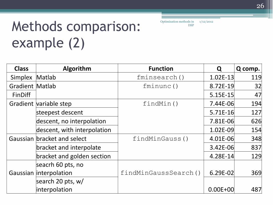
Methods comparison:
example (2)
1/12/2012Optimization methods in DSP
26
Class Algorithm Function Q Q comp.
Simplex Matlab fminsearch() 1.02E-13 119
Gradient Matlab fminunc() 8.72E-19 32
FinDiff 5.15E-15 47
Gradient variable step findMin() 7.44E-06 194
steepest descent 5.71E-16 127
descent, no interpolation 7.81E-06 626
descent, with interpolation 1.02E-09 154
Gaussian bracket and select findMinGauss() 4.01E-06 348
bracket and interpolate 3.42E-06 837
bracket and golden section 4.28E-14 129
Gaussianseacrh 60 pts, no interpolation findMinGaussSearch() 6.29E-02 369search 20 pts, w/ interpolation 0.00E+00 487

1/12/2012
27
Optimization methods in DSP

Practical considerations
• Limiting the search scope▫ Every engineering problem deal with limited parameter values
• Limiting the values of the internal variables
• Limiting the precision ▫ Don’t go for too small improvements
• Dealing with discrete values of the parameters▫ Use Gaussian search
• Dealing with the discrete values of the criterion▫ Modified min() function in Matlab
• Dynamic range of the variables▫ Scaling to magnitudes of 1’s or 10’s
1/12/2012Optimization methods in DSP
28

Training, development, and test sets
• Split the data corpus on three
• The training set is used to compute the optimization criterion
• The development set is computed after each iteration
• Test set is for the final evaluation
1/12/2012
29
Optimization methods in DSP
Number of iterations
Q
Qopt
Training set
Development set
Stop here!

Parallelization of the optimization
process• Parallelization:
▫ Running multiple threads on a multi-CPU and/or multicore-CPU
▫ Using a computing cluster
• Parallelization of the optimization criterion▫ Run job for each of the components of the data corpus
• Parallelization of the optimization process▫ Computing the gradient in parallel
▫ Doing search for many points at once Good for steepest gradient descent and Gaussian methods
• Parallelization has limits▫ Robust code with retries when some job fails
▫ Network search still takes a lot of time
1/12/2012
30
Optimization methods in DSP

1/12/2012
31
Optimization methods in DSP

Simple antenna filter
1/12/2012
32
Optimization methods in DSP
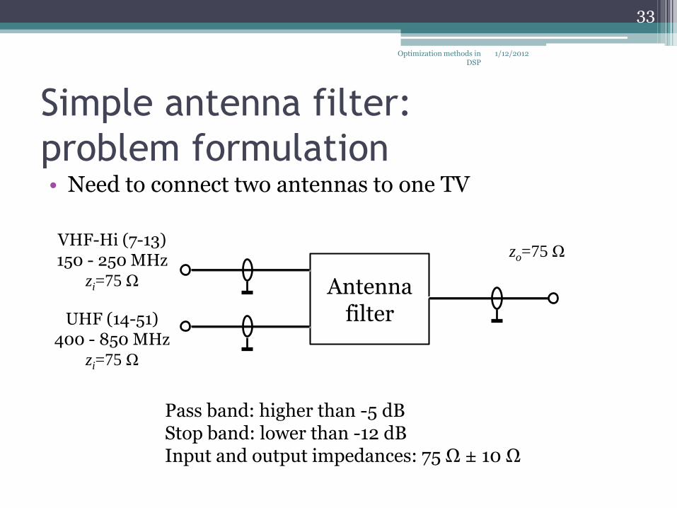
Simple antenna filter:
problem formulation• Need to connect two antennas to one TV
1/12/2012Optimization methods in DSP
33
Antenna filter
VHF-Hi (7-13)150 - 250 MHz
zi=75 Ω
UHF (14-51)400 - 850 MHz
zi=75 Ω
zo=75 Ω
Pass band: higher than -5 dBStop band: lower than -12 dBInput and output impedances: 75 Ω ± 10 Ω

102
103
-40
-35
-30
-25
-20
-15
-10
-5
0
5
Frequency, MHz
Tra
nsfe
r ra
tio
, d
B
Low pass filter
Simple antenna filter:
low pass filter
1/12/2012Optimization methods in DSP
34
L L
C
2 S
zL
F
2
2 S
CF z
zL
C
z = 75 Ω FS = 275 MHz
L = 43.4 nH
C = 15.4 pF10
210
30
50
100
150
Frequency, MHz
Inp
ut im
pe
da
nce
, O
hm
s
Low pass filter

102
103
-40
-35
-30
-25
-20
-15
-10
-5
0
5
Frequency, MHz
Tra
nsfe
r ra
tio
, d
B
High pass filterSimple antenna filter:
high pass filter
4 S
zL
F
1
2 S
CF z
zL
C
z = 75 Ω FS = 375 MHz
L = 15.9 nH
C = 5.7 pF
L
C C
102
103
0
50
100
150
Frequency, MHz
Inp
ut im
pe
da
nce
, O
hm
s
High pass filter
1/12/2012
35
Optimization methods in DSP

Simple antenna filter:
full diagram
1/12/2012Optimization methods in DSP
36
L1=47.7 nH
C1=16.9 pF
L2=47.7 nH
L3=17 nH
C2=6 pF C3=6 pF
Input 1150 - 250 MHz
zi=75 Ω
Input 2400 - 850 MHz
zi=75 Ω
Outputzo=75 Ω
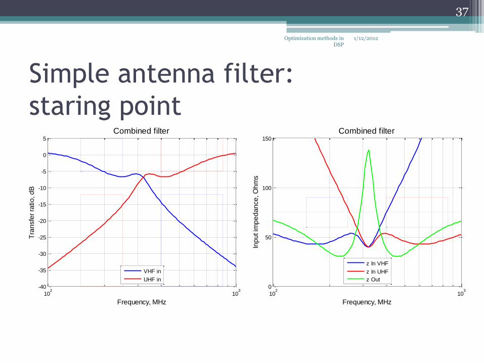
Simple antenna filter:
staring point
102
103
-40
-35
-30
-25
-20
-15
-10
-5
0
5
Frequency, MHz
Tra
nsfe
r ra
tio
, d
B
Combined filter
VHF in
UHF in
102
103
0
50
100
150
Frequency, MHz
Inp
ut im
pe
da
nce
, O
hm
s
Combined filter
z In VHF
z In UHF
z Out
1/12/2012
37
Optimization methods in DSP

Simple antenna filter:
optimization• Optimization parameters: L1, L2, C1, C2, C3, L3.
• Optimization criterion: weighted sum of 8 sub-criteria▫ Impedance match: VHF and UHF inputs, Output VHF, Output
UHF
▫ Frequency response: VHF and UHF inputs, stop and pass bands
▫ Weights: [0.1 0.1 2.0 2.0 20.0 10.0 20.0 10.0]
• Starting point: estimated with the filter design
• Constraints:▫
▫
• Q0 = 16.801, Qend = 2.898
3 300inH L nH
1 100ipF C pF
1/12/2012
38
Optimization methods in DSP

Simple antenna filter:
optimization results
L1=67.2 nH
C1=11.3 pF
L2=55.8 nH
L3=23.2 nH
C2=4.1 pF C3=5.5 pF
Input 1150 - 250 MHz
zi=75 Ω
Input 2400 - 850 MHz
zi=75 Ω
Outputzo=75 Ω
1/12/2012
39
Optimization methods in DSP

Simple antenna filter:
after optimization
102
103
-40
-35
-30
-25
-20
-15
-10
-5
0
5
Frequency, MHz
Tra
nsfe
r ra
tio
, d
B
Combined filter - optimized
VHF in
UHF in
102
103
0
50
100
150
Frequency, MHz
Inp
ut im
pe
da
nce
, O
hm
s
Combined filter - optimized
z In VHF
z In UHF
z Out
1/12/2012
40
Optimization methods in DSP

Simple antenna filter:
methods comparison
1/12/2012Optimization methods in DSP
41
Class Algorithm Function Q Q comp.
Simplex Matlab fminsearch() 2.965 826
Gradient Matlab fminunc() 2.964 1962
FinDiff 2.964 310
Gradient variable step findMin() 2.974 9507
steepest descent 2.976 5108
descent, no interpolation 2.976 9558descent, with interpolation 2.975 6764
Gaussian bracket and select findMinGauss() 2.921 279
bracket and interpolate 2.898 380
bracket and golden section 2.903 666
Gaussianseacrh 60 pts, no interpolation findMinGaussSearch() 2.986 1467search 20 pts, with interpolation 2.971 795

Noise suppressor optimization
1/12/2012
42
Optimization methods in DSP

Noise suppressor architecture
1/12/2012Optimization methods in DSP
43
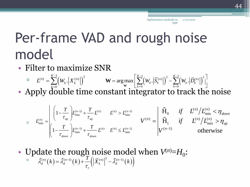
Per-frame VAD and rough noise
model• Filter to maximize SNR
▫• Apply double time constant integrator to track the noise
▫
• Update the rough noise model when V(n)=H0:▫
1/12/2012Optimization methods in DSP
44
1 12 2
( ) ( )
0 0
arg max . .K K
n n
k k k k
k k
W S W D
W
W 1 2
( ) ( )
0
.K
n n
k k
k
L W X
( ) ( )
0 min
( ) ( ) ( )
1 min
( 1)
H
H
otherwise
n n
down
n n n
up
n
if L L
V if L L
V
( 1) ( ) ( ) ( 1)
min min
( )
min
( 1) ( ) ( ) ( 1)
min min
1
1
n n n n
up upn
n n n n
down down
T TL L L L
LT T
L L L L
2( ) ( 1) ( ) ( 1)n n n n
d d k d
r
Tk k X k

Soft VAD and precise noise model
• From the PDFs of the noise p(Xk|H0) and the speech p(Xk|H1) compute the likelihood ratio (Sohn et all, 1998):
▫• Smooth using first order HMM
▫• Compute the speech presence probability
▫• Update the precise noise model
▫
1/12/2012Optimization methods in DSP
45
1
0
| H 1exp
| H 1 1
k k k
k
k k k
p X
p X
( 1)
( ) ( )01 11
( 1)
00 10
n
n nk
k kn
k
a a
a a
0( ) ( )
1
.n n
k k
P
P
( )
( )
( )1
n
n k
k n
k
P
2( ) ( 1) ( ) ( ) ( ) ( 1)
, , ,1 1 .n n n n n n
d k d k k k d k
p
TP P X

Suppression rules
• Prior and posterior SNRs:
▫
▫
• MMSE, Wiener (1947)
▫• Spectral subtraction, Boll (1975):
• Maximum Likelihood, McAulay & Malpass (1981):
▫
1/12/2012Optimization methods in DSP
46
( )
( ) ( ) 1
s k
k
s d k
kH
k k
2
( ),
( ) ( )
ks
k k
d d
Xk
k k
2( )d kk E D 2
( )s kk E S
1
kk
k
H
1 1
2 2 1
kk
k
H
0 0.5 1 1.5 2 2.5 3 3.5 4 4.5 50
0.1
0.2
0.3
0.4
0.5
0.6
0.7
0.8
0.9
1
Winer, spectral subtraction and ML suppression rules
a posteriori SNR k
Su
pp
ressio
n r
ule
Hk ,
dB
Wiener
Spectral subtrcation
Max likelihood

-30
-20
-10
0
10
20
30 -30-20
-100
1020
30
-5
0
5
a priori SNR k
, dB
Comparision MMSE and log-MMSE rules
a posteriori SNR k
, dB
Diffe
ren
ce
, d
B
Suppression rules (2)
• ST-MMSE, Ephraim & Malah (1984):
▫
▫
• ST-logMMSE, Ephraim & Malah (1985):
▫
• Efficient alternatives, Wolfe&Godsill (2001):▫ Joint Maximum A Posteriori Spectral
Amplitude and Phase (JMAP SAP) Estimator▫ Maximum A Posteriori Spectral Amplitude
(MAP SA) Estimator▫ MMSE Spectral Power (MMSE SP) Estimator
1/12/2012Optimization methods in DSP
47
0 11 I I exp2 2 2 2
k k k kk k k
k
H
1 exp( )
1 2k
kk
k
tH dt
t
-30
-20
-10
0
10
20
30 -30-20
-100
1020
30
-30
-20
-10
0
10
20
a priori SNR k
, dB
Ephraim and Malah log-MMSE rule
a posteriori SNR k
, dB
Su
pp
ressio
n r
ule
Hk ,
dB
( )1
kk
k
k

Prior SNR estimation and rule modifier
• Prior SNR using decision directed approach, Ephraim & Malah(1984):
▫
• Uncertain presence of the speech signal▫ Pauses are integral part of the speech signal▫ McAulay & Malpass (1981):
▫ Ephraim & Malah (1984):
▫ Middleton & Esposito (1968)
1/12/2012Optimization methods in DSP
48
2( 1)
( ) ( )
( )
ˆ
1 .max 0, 1
n
kn n
k kn
d
S
( ) ( ) ( ).n n n
k k kH P H
,.
1 ,
k k
k k
k k
X qH H
X q
1
0
| H,
| H
k
k k k
k
P XY q
P X 1 /k k kq q

Practical aspects
• Avoid division by zero : ▫ Check for, or add a small constant
• Avoid overflow: ▫ exp(max(700,x))
▫ ln(x+ε)
• Limit the values in realistic boundaries:▫ probabilities [0.001,0.999], etc.
• Smooth in time▫ First order integrator
▫ HMM based
• Limiting suppression gains ▫
1/12/2012Optimization methods in DSP
49
( ) ( ) ( )1 1n n n
k Um Um k m m kH G G P G G H

Tuning as optimization problem
• Numerous parameters that can’t be computed▫ Adaptation time constants, thresholds, feedback parameters
• Formulate good optimization criterion▫ “Better” noise suppressor? SNR? MMSE? LSD? ML? log-MMSE?
We actually don’t want MMSE, or ML, or even log-MMSE estimators
We want humans to perceive the output signal as “better” quality
▫ Perceptual quality
Mean Opinion Score (MOS), ITU.T Recommendation P.800
Perceptual Evaluation of Sound Quality (PESQ)
Computational proxy of MOS measurements
ITU-T Recommendation P.864.2
▫ Combined optimization criterion:
Q = w1*PESQ + w2*SNR - w3*LSD - w4*MMSE
1/12/2012Optimization methods in DSP
50

Tuning as optimization problem (2)
• Generate proper data corpus (synthetic vs. real recordings)▫ Measure the impulse responses between various positions of the
driver’s head (9) and microphone (12)
▫ Record noise corpus under various driving conditions (5x3)
▫ Clean speech corpus: TMIT (6300 utterances)
▫ Combine randomly, correct for the Lombard effect, split on 3
• Perform the optimization▫ Gaussian minimization
▫ Parallelized for execution on 240 CPUs
• See Tashev, Lovitt, Acero – PacRim 2009 for details
1/12/2012Optimization methods in DSP
51

Tuning as optimization problem (2)
• Generate proper data corpus (synthetic vs. real recordings)▫ Measure the impulse responses between various positions of the
driver’s head (9) and microphone (12)
▫ Record noise corpus under various driving conditions (5x3)
▫ Clean speech corpus: TMIT (6300 utterances)
▫ Combine randomly, correct for the Lombard effect, split on 3
• Perform the optimization▫ Gaussian minimization
▫ Parallelized for execution on 240 CPUs
• See Tashev, Lovitt, Acero – PacRim 2009 for details
1/12/2012Optimization methods in DSP
52

Tuning as optimization problem (2)
• Generate proper data corpus (synthetic vs. real recordings)▫ Measure the impulse responses between various positions of the
driver’s head (9) and microphone (12)
▫ Record noise corpus under various driving conditions (5x3)
▫ Clean speech corpus: TMIT (6300 utterances)
▫ Combine randomly, correct for the Lombard effect, split on 3
• Perform the optimization▫ Gaussian minimization
▫ Parallelized for execution on 240 CPUs
• See Tashev, Lovitt, Acero – PacRim 2009 for details
1/12/2012Optimization methods in DSP
53

Results
• Suppression rule independent parameters
• Suppression rules
1/12/2012Optimization methods in DSP
54
0.035 20.0 1.1 2.9 1.39 0.825 0.37 0.11 0.41 0.73 0.940 0.974
down updown up
r p 01a 10a 01b 10b VAD
Rule PESQ SNR MSE LSD Gm GUm
Base line 2.449 7.62 0.718820 7.654
MMSE 2.839 22.11 0.434427 9.410 0.329 0.092
MMSE DDA 3.020 31.58 0.419704 10.256 0.020 0.100
ML 2.795 19.24 0.457038 8.188 0.001 0.018
SS 2.983 25.02 0.421912 9.394 0.001 0.083
ST-MMSE 3.003 28.15 0.419987 9.316 0.024 0.100
ST log-MMSE 3.018 30.49 0.420202 9.797 0.001 0.103
JMAP SAP 3.011 28.18 0.419490 9.392 0.020 0.100
MAP SAE 3.021 29.42 0.419297 9.640 0.020 0.100
MMSE SP 3.011 28.70 0.419637 9.468 0.001 0.097
Improvements:
0.57 – baseline
0.17-0.27 – industrial
(in PESQ points)
20-22 dBC – baseline
10-14 dBC – industrial
(in SNR)

Audio pipeline in Kinect
1/12/2012Optimization methods in DSP
55

Audio pipeline architecture
1/12/2012Optimization methods in DSP
56
AECBF
Microphone Array
AES NSAECAECCTR
Calib-ration
AECAECAECMAEC AGC
SSL
Echo Est.
VAD
Surround sound output
Direction, confidence
Audio pipeline output
To all blocks

End-to-end optimization
• Mean Opinion Score (MOS) and Perceptual Evaluation of Sound Quality (PESQ)
• 75 parameters for optimization
• Optimization criterion:▫ Q = PESQ+0.01*ERLE+0.001*SNR-0.001*LSD-0.01*MSE
• Optimization algorithm▫ Gaussian minimization
• Data corpus with various distance, levels, reverberation
• Parallelized processing on computing cluster, 216 CPUs
• Optimization time: ~50 hours
1/12/2012Optimization methods in DSP
57

End-to-end optimization: results
1/12/2012Optimization methods in DSP
58
0
10
20
30
40
50
60
70
80
90
100
0 20 40 60 80 100
Imp
ro
ve
me
nts
in
WE
R,
%
Loudspeaker volume, %
Multi-volume recognition results
Do nothing
Before optim
After optim
After training
Speech NUI goodup to here
Supported levelsup to here

Results: demo
1/12/2012Optimization methods in DSP
59
AECBF
Microphone Array
AES NSAECAECCTR
Calib-ration
AECAECAECMAEC AGC
SSL
Echo Est.
VAD
Surround sound output
Direction, confidence
Audio pipeline output
To all blocks

1/12/2012
60
Optimization methods in DSP
Conclusions
• Optimization methods are powerful tool for improving the parameters of complex DSPsystems
• Your data corpus is the model of the world you want your system to work – it is not going to work in conditions not in the corpus
• Use training, development, and test data
• Don’t chase the mathematical optimum, use engineering precision and common sense
1/12/2012
61
Optimization methods in DSP

Shameless plug-in #1
Ivan Tashev. Sound Capture and Processing: Practical Approaches. Willey, 2009
Contains algorithms, a lot of figures, and sample Matlab code
1/12/2012Optimization methods in DSP
62
Shameless plug-in #2
Saturday, January 14
10:15 – 10:45, Milano I
“Audio for Kinect: nearly impossible”Dr. Ivan Tashev, Microsoft Research
1/12/2012
63
Optimization methods in DSP

References
• W. Press, S. Teukolsky, W. Vetterling, B. Flannery. Numerical Recipes in C++, Cambridge University Press, 2002.
• A. Antoniou, W.-S. Lu. Practical Optimization, Springer, 2007.
• T. Shoup. A Practical Guide to Computer Methods for Engineers, Prentice Hall, 1979.
• R. P. Brent. Algorithms for Minimization without Derivatives, Prentice Hall, 1973.
• J. E. Dennis, R. B. Schnabel. Numerical Methods for Unconstrained Optimization and Nonlinear Equations, SIAM, 1983.
• D. A. H. Jacobs. The State of the Art in Numerical Analysis, Academic Press, 1977.
• S. Boyd, L. Vandenberghe. Convex Optimization, Cambridge University Press, 2004
1/12/2012Optimization methods in DSP
64

Finally
Questions?
Bring your USB memory sticks to copy the Matlabsoftware!
Contact info:[email protected]
http://research.microsoft.com/en-us/people/ivantash/
1/12/2012
65
Optimization methods in DSP