OPTIMAL RESOURCE ALLOCATION AND CROSS-LAYER CONTROL IN

COGNITIVE AND COOPERATIVE WIRELESS NETWORKS

by

Rahul Urgaonkar

A Dissertation Presented to theFACULTY OF THE USC GRADUATE SCHOOLUNIVERSITY OF SOUTHERN CALIFORNIA

In Partial Fulfillment of theRequirements for the Degree

DOCTOR OF PHILOSOPHY(ELECTRICAL ENGINEERING)

May 2011

Copyright 2011 Rahul Urgaonkar

Dedication

To Aai-Baba, BB, and Paulami

ii

Acknowledgments

This work would not have been possible without the encouragement, help, and guidance

that I received over the years from many individuals. First and foremost is my advisor,

Prof. Michael J. Neely. I remember attending a seminar talk that he gave at USC as

a new faculty member sometime in early 2004. At that time, I was a Master’s student,

barely contemplating the idea of pursuing a Ph.D. I still remember the sense of awe that

I felt listening to him talk about his doctoral work. I thought that if I were to ever

pursue a Ph.D., this is the kind of research I would want to do. I am forever grateful

to Prof. Neely for taking me as his student and patiently helping me through thick and

thin, from being a role model and a guide to sharing his candid assessments of my work

and providing valuable feedback. I hope I have been able to achieve at least some of what

I set out to do in my work.

I would like to express my sincere thanks to Prof. Bhaskar Krishnamachari who was

my research advisor during my Master’s studies and who served on my committee. It

was with Bhaskar that I got the first opportunity to do research in the area of Wireless

Networks. His enthusiasm for research, learning, and mentoring students is truly inspiring

and I feel lucky to have benefitted from that. I am also thankful to my other committee

iii

members: Prof. Giuseppe Caire, Prof. Leana Golubchik, Prof. Keith M. Chugg, and

Prof. C.-C. Jay Kuo for their time.

Working in the Communication Sciences Institute was made memorable by my friends

and colleagues Ozgun, Chih-ping, and Longbo as well as Gerrie, Anita, Mayumi, and

Milly. I also thank Apoorva, my room-mate for several years, and Sumit and Anant, for

their friendship. I wish everyone the best in all future endeavors of their lives.

My family has been the constant force supporting me religiously in my darkest hours.

I could count on them to discuss with me at any hour what now seem the most trivial of

all “problems”. My parents, Narendra and Dr. Charu Urgaonkar, have been my greatest

fans and this work is dedicated to them. My brother, Prof. Bhuvan Urgaonkar has been

a role model and a friend whose advice has helped me in innumerable ways. I am also

thankful to my Uncle and Aunt, Dr. Mohan and Shachi Gawande and my grandfather,

Dr. Trimbak Gawande for providing me a home away from home.

Last, but not the least of all who helped me jump “The Fence” is my best friend,

my dear wife Paulami whose love for me knows no bounds. The best thing that ever

happened to me was meeting with her. Thank you Paulami, for making every day with

you an adventure!

Rahul Urgaonkar

March 2011

iv

Table of Contents

Dedication ii

Acknowledgments iii

List of Figures viii

Abstract x

Chapter 1: Introduction 11.1 Models for Cognitive Radio Networks . . . . . . . . . . . . . . . . . . . . 31.2 Summary of Contributions . . . . . . . . . . . . . . . . . . . . . . . . . . . 51.3 Outline of Thesis . . . . . . . . . . . . . . . . . . . . . . . . . . . . . . . . 8

Chapter 2: Reliable Scheduling in Cognitive Radio Networks 92.1 Introduction . . . . . . . . . . . . . . . . . . . . . . . . . . . . . . . . . . . 102.2 Network Model . . . . . . . . . . . . . . . . . . . . . . . . . . . . . . . . . 12

2.2.1 Mobility Model . . . . . . . . . . . . . . . . . . . . . . . . . . . . . 132.2.2 Interference Model . . . . . . . . . . . . . . . . . . . . . . . . . . . 142.2.3 Primary User Traffic Model . . . . . . . . . . . . . . . . . . . . . . 162.2.4 Channel State Information Model . . . . . . . . . . . . . . . . . . 172.2.5 Queueing Dynamics and Control Decisions . . . . . . . . . . . . . 202.2.6 Discussion of Network Model . . . . . . . . . . . . . . . . . . . . . 21

2.3 Maximum Throughput Objective . . . . . . . . . . . . . . . . . . . . . . . 222.4 Optimal Control Algorithm . . . . . . . . . . . . . . . . . . . . . . . . . . 24

2.4.1 Cognitive Network Control Algorithm (CNC) . . . . . . . . . . . . 252.4.2 Comparison with a Counter Based Algorithm . . . . . . . . . . . . 282.4.3 Performance Analysis . . . . . . . . . . . . . . . . . . . . . . . . . 31

2.5 Stochastic Lyapunov Optimization . . . . . . . . . . . . . . . . . . . . . . 352.5.1 Lyapunov Drift . . . . . . . . . . . . . . . . . . . . . . . . . . . . . 372.5.2 Optimal Stationary, Randomized Policy . . . . . . . . . . . . . . . 39

2.6 Distributed Implementation . . . . . . . . . . . . . . . . . . . . . . . . . . 422.7 Simulations . . . . . . . . . . . . . . . . . . . . . . . . . . . . . . . . . . . 452.8 Chapter Summary . . . . . . . . . . . . . . . . . . . . . . . . . . . . . . . 47

v

Chapter 3: Delay-Limited Cooperative Communication 493.1 Introduction . . . . . . . . . . . . . . . . . . . . . . . . . . . . . . . . . . . 503.2 Basic Network Model . . . . . . . . . . . . . . . . . . . . . . . . . . . . . . 55

3.2.1 Example of Channel State Information Models . . . . . . . . . . . 573.2.2 Control Options . . . . . . . . . . . . . . . . . . . . . . . . . . . . 583.2.3 Discussion of Basic Model . . . . . . . . . . . . . . . . . . . . . . . 61

3.3 Control Objective . . . . . . . . . . . . . . . . . . . . . . . . . . . . . . . . 623.4 Optimal Control Algorithm . . . . . . . . . . . . . . . . . . . . . . . . . . 643.5 Known Channels, Unknown Statistics . . . . . . . . . . . . . . . . . . . . 70

3.5.1 Regenerative DF, Orthogonal Channels . . . . . . . . . . . . . . . 723.5.2 Non-Regenerative DF, Orthogonal Channels . . . . . . . . . . . . . 753.5.3 AF, Orthogonal Channels . . . . . . . . . . . . . . . . . . . . . . . 763.5.4 DF with DSTC . . . . . . . . . . . . . . . . . . . . . . . . . . . . . 783.5.5 AF with DSTC . . . . . . . . . . . . . . . . . . . . . . . . . . . . . 80

3.6 Unknown Channels, Known Statistics . . . . . . . . . . . . . . . . . . . . 813.6.1 Simulation Based Method . . . . . . . . . . . . . . . . . . . . . . . 82

3.7 Multi-Source Extensions . . . . . . . . . . . . . . . . . . . . . . . . . . . . 843.8 Simulations . . . . . . . . . . . . . . . . . . . . . . . . . . . . . . . . . . . 863.9 Chapter Summary . . . . . . . . . . . . . . . . . . . . . . . . . . . . . . . 90

Chapter 4: Opportunistic Cooperation in Cognitive Networks 914.1 Introduction . . . . . . . . . . . . . . . . . . . . . . . . . . . . . . . . . . . 924.2 Basic Model . . . . . . . . . . . . . . . . . . . . . . . . . . . . . . . . . . . 96

4.2.1 Control Decisions and Queueing Dynamics . . . . . . . . . . . . . 994.2.2 Control Objective . . . . . . . . . . . . . . . . . . . . . . . . . . . 101

4.3 Solution Using The “Drift-plus-Penalty” Ratio Method . . . . . . . . . . . 1044.4 The Maximizing Policy of (4.16) . . . . . . . . . . . . . . . . . . . . . . . 107

4.4.1 Proof Details . . . . . . . . . . . . . . . . . . . . . . . . . . . . . . 1094.5 Performance Analysis . . . . . . . . . . . . . . . . . . . . . . . . . . . . . 1164.6 Extensions to Basic Model . . . . . . . . . . . . . . . . . . . . . . . . . . . 120

4.6.1 Multiple Secondary Users . . . . . . . . . . . . . . . . . . . . . . . 1204.6.2 Fading Channels . . . . . . . . . . . . . . . . . . . . . . . . . . . . 123

4.7 Simulations . . . . . . . . . . . . . . . . . . . . . . . . . . . . . . . . . . . 1294.8 Chapter Summary . . . . . . . . . . . . . . . . . . . . . . . . . . . . . . . 132

Chapter 5: Optimal Routing with Mutual Information Accumulation 1345.1 Introduction . . . . . . . . . . . . . . . . . . . . . . . . . . . . . . . . . . . 1355.2 Network Model . . . . . . . . . . . . . . . . . . . . . . . . . . . . . . . . . 1395.3 Minimum Delay Routing . . . . . . . . . . . . . . . . . . . . . . . . . . . . 141

5.3.1 Timeslot and Transmission Structure . . . . . . . . . . . . . . . . . 1415.3.2 Problem Formulation . . . . . . . . . . . . . . . . . . . . . . . . . 1435.3.3 Characterizing the Optimal Solution of (5.1) . . . . . . . . . . . . 1455.3.4 Proof of Theorem 6 . . . . . . . . . . . . . . . . . . . . . . . . . . 1475.3.5 Exact Solution for a Line Network . . . . . . . . . . . . . . . . . . 154

5.4 Minimum Energy Routing with Delay Constraint . . . . . . . . . . . . . . 156

vi

5.4.1 Problem Formulation . . . . . . . . . . . . . . . . . . . . . . . . . 1575.4.2 Characterizing the Optimal Solution of (5.9) . . . . . . . . . . . . 1585.4.3 A Greedy Algorithm . . . . . . . . . . . . . . . . . . . . . . . . . . 161

5.5 Minimum Delay Broadcast . . . . . . . . . . . . . . . . . . . . . . . . . . 1625.5.1 Timeslot and Transmission Structure . . . . . . . . . . . . . . . . . 1625.5.2 Problem Formulation . . . . . . . . . . . . . . . . . . . . . . . . . 1635.5.3 Characterizing the Optimal Solution of (5.10) . . . . . . . . . . . . 1645.5.4 Proof of Theorem 9 . . . . . . . . . . . . . . . . . . . . . . . . . . 1655.5.5 A Greedy Algorithm . . . . . . . . . . . . . . . . . . . . . . . . . . 168

5.6 Distributed Heuristics and Simulations . . . . . . . . . . . . . . . . . . . . 1695.6.1 Simulation Results . . . . . . . . . . . . . . . . . . . . . . . . . . . 170

5.7 Chapter Summary . . . . . . . . . . . . . . . . . . . . . . . . . . . . . . . 173

Chapter 6: Conclusions 175

Bibliography 178

Appendix AAppendices for Chapter 2 . . . . . . . . . . . . . . . . . . . . . . . . . . . . . . 186A.1 Lyapunov Drift under policy STAT . . . . . . . . . . . . . . . . . . . . . . 186A.2 Convergence of Markov Chains . . . . . . . . . . . . . . . . . . . . . . . . 188A.3 On Greedy Maximal Weight Matchings . . . . . . . . . . . . . . . . . . . 188

Appendix BAppendices for Chapter 3 . . . . . . . . . . . . . . . . . . . . . . . . . . . . . . 190B.1 Proof of Theorem 4 . . . . . . . . . . . . . . . . . . . . . . . . . . . . . . . 190B.2 Solution to (3.17) using KKT conditions . . . . . . . . . . . . . . . . . . . 191B.3 Solution to (3.21) using KKT conditions . . . . . . . . . . . . . . . . . . . 192

Appendix CAppendices for Chapter 4 . . . . . . . . . . . . . . . . . . . . . . . . . . . . . . 193C.1 Proof of Lemma 3 . . . . . . . . . . . . . . . . . . . . . . . . . . . . . . . 193C.2 Proof of Theorem 5, parts (2) and (3) . . . . . . . . . . . . . . . . . . . . 195C.3 Computing D . . . . . . . . . . . . . . . . . . . . . . . . . . . . . . . . . . 197

Appendix DAppendices for Chapter 5 . . . . . . . . . . . . . . . . . . . . . . . . . . . . . . 199D.1 Proof of Lemma 4 . . . . . . . . . . . . . . . . . . . . . . . . . . . . . . . 199D.2 Proof of Lemma 5 . . . . . . . . . . . . . . . . . . . . . . . . . . . . . . . 199D.3 A Simple Example . . . . . . . . . . . . . . . . . . . . . . . . . . . . . . . 200

vii

List of Figures

2.1 Example cognitive network showing primary and secondary users . . . . . 13

2.2 Two state Markov Chain example for primary user channel occupancyprocess . . . . . . . . . . . . . . . . . . . . . . . . . . . . . . . . . . . . . . 16

2.3 Total average congestion vs. input rate under the Counter Based Algo-rithm and CNC. . . . . . . . . . . . . . . . . . . . . . . . . . . . . . . . . 29

2.4 Example cell-partitioned network used in simulation . . . . . . . . . . . . 45

2.5 Total average congestion vs. input rate for different values of V . . . . . . 48

2.6 Achieved throughput vs. input rate for different values of V . . . . . . . . 48

3.1 Example 2-hop network with source, destination and relays. The time slotstructures for different transmission strategies are also shown. Due to thehalf-duplex constraint, cooperative protocols need to operate in two phases. 51

3.2 A snapshot of the example network used in simulation. . . . . . . . . . . . 87

3.3 Average Sum Power vs. V. . . . . . . . . . . . . . . . . . . . . . . . . . . 88

3.4 Average Reliability Queue Occupancy vs. V. . . . . . . . . . . . . . . . . 89

4.1 Example femtocell network with primary and secondary users. . . . . . . 96

4.2 Frame-based structure of the problem under consideration. Each frameconsists of two periods: PU Idle and PU Busy. . . . . . . . . . . . . . . . 97

4.3 Birth-Death Markov Chain over the system state where the system staterepresents the primary user queue backlog. . . . . . . . . . . . . . . . . . 110

4.4 Average Secondary User Throughput vs. V. . . . . . . . . . . . . . . . . . 130

viii

4.5 Average Secondary User Queue Occupancy vs. V. . . . . . . . . . . . . . 131

4.6 Moving Average of Secondary User Throughput over Frames. . . . . . . . 133

4.7 Moving Average of Power used by the Secondary User for CooperativeTransmissions over Frames. . . . . . . . . . . . . . . . . . . . . . . . . . . 133

5.1 Example network with source, destination and 4 relay nodes. When anode transmits, every other node that has not yet decoded the packetaccumulates mutual information at a rate given by the capacity of the linkbetween the transmitter and that node. . . . . . . . . . . . . . . . . . . . 140

5.2 Example timeslot and transmission structure. In each stage, nodes thathave already decoded the full packet transmit on orthogonal channels intime. . . . . . . . . . . . . . . . . . . . . . . . . . . . . . . . . . . . . . . . 142

5.3 Optimal timeslot and transmission structure. In each stage, only the nodethat decodes the packet at the beginning of that stage transmits. . . . . . 145

5.4 A line network. . . . . . . . . . . . . . . . . . . . . . . . . . . . . . . . . . 154

5.5 Optimal timeslot and transmission structure for minimum delay broadcast.In each stage, at most one node from the set of nodes that have the fullpacket transmits. . . . . . . . . . . . . . . . . . . . . . . . . . . . . . . . . 165

5.6 A 25 node network where the routes for traditional minimum delay, Heuris-tics 1 and 2, and optimal mutual information accumulation are shown. . . 171

5.7 The CDF of the ratio of the minimum delay under the two heuristics andthe traditional shortest path to the minimum delay under the optimalmutual information accumulation solution. . . . . . . . . . . . . . . . . . . 172

D.1 The 4 node example network used in Appendix D.3. . . . . . . . . . . . . 200

ix

Abstract

We investigate four problems on optimal resource allocation and cross-layer control in

cognitive and cooperative wireless networks with time-varying channels. The first three

problems consider different models and capabilities associated with cognition and coop-

eration in such networks. Specifically, the first problem focuses on the dynamic spectrum

access model for cognitive radio networks and assumes no cooperation between the li-

censed (or “primary”) and unlicensed (or “secondary”) users. Here, the secondary users

try to avoid interfering with the primary users while seeking transmission opportunities

on vacant primary channels in frequency, time, or space. The second problem considers

a relay-based fully cooperative wireless network. Here, cooperative communication tech-

niques at the physical layer are used to improve the reliability and energy cost of data

transmissions. The third problem considers a cooperative cognitive radio network where

the secondary users can cooperatively transmit with the primary users to improve the

latter’s effective transmission rate. In return, the secondary users get more opportunities

for transmitting their own data when the primary users are idle.

In all of these scenarios, our goal is to design optimal control algorithms that maximize

time-average network utilities (such as throughput) subject to time-average constraints

(such as power, reliability, etc.). To this end, we make use of the technique of Lyapunov

x

optimization to design online control algorithms that can operate without requiring any

knowledge of the statistical description of network dynamics (such as fading channels,

node mobility, and random packet arrivals) and are provably optimal. The algorithms for

the first two problems use greedy decisions over one slot and two-slot frames, whereas the

algorithm for the third problem involves a stochastic shortest path decision over a variable

length frame, and this is explicitly solved, remarkably without requiring knowledge of the

network arrival rates.

Finally, in the fourth problem, we investigate optimal routing and scheduling in static

wireless networks with rateless codes. Rateless codes allow each node of the network to

accumulate mutual information with every packet transmission. This enables a significant

performance gain over conventional shortest path routing. Further, it also outperforms

cooperative communication techniques that are based on energy accumulation. However,

it requires complex and combinatorial networking decisions concerning which nodes par-

ticipate in transmission, and which decode ordering to use. We formulate the general

problems as combinatorial optimization problems and identify several structural proper-

ties of the optimal solutions. This enables us to derive optimal greedy algorithms to solve

these problems. This work uses a different set of tools and can be read independently of

the other chapters.

xi

Chapter 1

Introduction

Next generation wireless networks are expected to provide significantly higher data rates,

reliability, and energy efficiency than the current systems. There has been much effort in

recent years to develop new techniques that improve the performance of wireless networks

to achieve these objectives. Cognitive radio and cooperative communication are two

important examples of such emerging techniques.

The motivation for cognitive radios comes from the observation that the existing static

allocation of spectrum to licensed (or “primary”) users leads to inefficient utilization and

creates spectrum scarcity. By allowing unlicensed (or “secondary”) wireless devices to

dynamically access the unused portions of the spectrum, it is possible to support more

users in the existing spectrum and improve its spectral efficiency. However, such dy-

namic spectrum access may cause undesirable interference to the licensed users. Thus,

it is important to design opportunistic scheduling schemes that provide strong reliability

guarantees for the licensed users while attempting to maximize the utility (e.g., through-

put) of the unlicensed users.

1

The motivation for cooperative communication comes from the work on MIMO sys-

tems which shows that deploying multiple antennas on wireless devices offers substantial

performance improvements. However, this may be infeasible is small-sized devices due

to space limitations. Cooperative communication (“network MIMO”) tries to emulate

the gains of traditional MIMO systems in a distributed network of single antenna nodes.

This form of communication transforms the traditional node or link based problems of

resource allocation into a network wide problem. This necessitates the design of oppor-

tunistic algorithms that make use resources (such as power) fairly across all users to

achieve a target performance.

The technique of cooperative communication can be used to obtain further gains in

cognitive radio networks that go beyond the traditional dynamic spectrum access model.

In this model, the secondary users try to avoid interfering with the primary users while

seeking transmission opportunities on vacant primary channels. This model assumes no

cooperation between the primary and secondary users. However, with cooperative com-

munication, a secondary user can use its resources to improve the effective transmission

rate of the primary user. In return, the secondary user can get more opportunities for

transmitting its own data when the primary user is idle. In this scenario, the secondary

users need to make dynamic decisions on whether to cooperate or not in order to maximize

their transmission opportunities.

In this thesis, we study several such resource allocation problems in the area of cog-

nition and cooperation in wireless networks. Our goal is to design optimal control algo-

rithms that maximize general time-average network utilities (such as throughput) subject

2

to time-average constraints (such as power, reliability, etc.). We describe these problems

in more detail in Sec. 1.2.

1.1 Models for Cognitive Radio Networks

Several different models for cognitive radio networks have been considered in the lit-

erature. Depending on the assumptions made about the capabilities of cognition and

cooperation and the method of secondary user transmissions, these can be broadly clas-

sified under the following three categories [GJMS09]:

1. Underlay Model: In this model, the secondary users are allowed to transmit

concurrently with the primary users as long as the resulting interference caused to

the primary receivers is below some acceptable threshold. This may be achieved,

for example, using ultrawideband (UWB) transmissions where the secondary users

transmit over a wide bandwidth such that the resulting interference power at the

primary receivers is below the noise floor. Since the primary interference constraints

are typically quite restrictive, the secondary users are limited to short range com-

munication in this model.

2. Overlay Model: In this model, it is assumed that the secondary users are aware

of the primary user codebooks and possibly its messages. This knowledge can

then be exploited by the secondary user to either mitigate or altogether cancel any

interference seen at the primary and secondary receivers. This may be achieved

using sophisticated coding and interference management techniques such as Dirty

Paper Coding and Interference Alignment. While this model can potentially achieve

3

the largest rate region, the assumption about non-causal knowledge of primary

messages at the secondary user may limit its practical utility.

3. Interweave Model: This model is inspired by the notion of opportunistic com-

munication where the secondary users seek transmission opportunities in vacant

primary channels in frequency, time, and/or space, also knows as “spectrum holes”.

Also referred to as the dynamic spectrum access model, here the secondary users

monitor the spectrum occupancy process of the primary users and then opportunis-

tically transmit on idle primary channels. A key challenge here is to maximize such

opportunities while limiting the interference caused to the primary users due to

imperfect knowledge of the primary user channel occupancy state.

In this thesis, we will focus primarily on the Interweave Model. Within this model,

several variants have been considered in the literature that differ in the assumptions

made on the interaction between the primary and secondary users in the network. See,

for example, [Bud07, ZS07] for surveys on the taxonomy and classifications for such dy-

namic spectrum access networks. On one extreme is the case where the primary users

are completely oblivious to the secondary users and do not change their spectrum usage

to accommodate them. In this case, it is the responsibility of the secondary users to

avoid interfering excessively with the primary users by intelligently monitoring the spec-

trum and transmitting opportunistically. On the other extreme is the case where the

primary and secondary users fully cooperate in each other’s transmissions (for example,

using relay-based cooperative communication). There can also be hybrid scenarios where

the primary users are aware of the presence of secondary users, but do not spend their

4

resources helping secondary transmissions. We consider all of these scenarios in Chapters

2, 3, and 4 respectively, as discussed next.

1.2 Summary of Contributions

In this thesis, we study the following problems on optimal resource allocation and cross-

layer control in cognitive and cooperative wireless networks:

1. In Chapter 2, we consider a cognitive network with licensed (primary) users and un-

licensed (secondary) users under the dynamic spectrum access model. The primary

users are assumed to be completely oblivious to the presence of the secondary users.

The secondary users have imperfect knowledge about the primary users’ spectrum

usage and must meet a constraint on the maximum time-average rate of collisions

for each primary user while seeking transmission opportunities on the primary chan-

nels. We formulate this as a constrained stochastic optimization problem. In order

to satisfy the maximum collision constraint, we make use of the virtual cost queue

technique of [Nee06] in the form of “collision” queues. These collision queues enable

stochastic optimization by acting as dynamic Lagrange multipliers [HN09]. Using

the technique of Lyapunov optimization, we design an online admission control,

scheduling and resource allocation algorithm that meets the desired objectives and

provides explicit performance guarantees. This algorithm works in the presence of

imperfect knowledge about the primary user spectrum usage and does not require

5

knowledge of the secondary user mobility patterns. A salient feature of our algo-

rithm is that it provides deterministic worst case bounds on the maximum number

of collisions suffered by a primary user over any time duration.

2. In Chapter 3, we investigate optimal resource allocation for delay-limited coopera-

tive communication in time varying wireless networks. Specifically, we consider a

team of mobile users with real-time applications that have strict delay constraints

and fixed rate and reliability requirements (e.g., voice, multimedia). Cooperative

communication is particularly attractive in such delay-limited scenarios since it can

offer significant spatial diversity gains on top of conventional techniques used for

combating fading. In this chapter, we develop dynamic cooperation strategies that

make optimal use of network resources to achieve a target outage probability (reli-

ability) for each user subject to average power constraints. Using the technique of

Lyapunov optimization, we first present a general framework to solve this problem

and then derive quasi-closed form solutions for several cooperative protocols pro-

posed in the literature (such as Decode-and-Forward and Amplify-and-Forward).

Both scenarios where channel state information is available at the transmitter and

when only the statistics are known are considered. The model studied in this chap-

ter can be considered as a fully cooperative cognitive network where there is no

distinction between the primary and secondary users.

3. In Chapter 4, we extend the model of a cognitive radio network introduced in Chap-

ter 2 and allow a secondary user to cooperate with the primary user in order to

improve the reliability of the primary transmissions. Although the secondary user

6

must use its own resources for such cooperation, the observation is that this po-

tentially creates more opportunities for the secondary user to transmit its data.

However, the secondary user must balance the desire to cooperate more (to create

more transmission opportunities) with the need for maintaining sufficient energy

levels for its own transmissions. Such a model is applicable in the emerging area

of cognitive femtocell networks. We formulate the problem of maximizing the sec-

ondary user throughput subject to a time average power constraint under these

settings. This is a constrained Markov Decision Problem and conventional solution

techniques based on dynamic programming require either extensive knowledge of

the system dynamics or learning based approaches that suffer from large conver-

gence times. However, using the technique of Lyapunov optimization, we design a

novel greedy and online control algorithm that overcomes these challenges and is

provably optimal.

4. In Chapter 5, we consider the problem of optimal routing and scheduling strategies

for multi-hop wireless networks with rateless codes. Rateless codes allow each node

of the network to accumulate mutual information with every packet transmission.

This enables a significant performance gain over conventional shortest path routing.

Further, it also outperforms cooperative communication techniques that are based

on energy accumulation. However, it requires complex and combinatorial network-

ing decisions concerning which nodes participate in transmission, and which decode

ordering to use. We formulate the general problem as a combinatorial optimization

problem and then make use of several structural properties to simplify the solution

7

and derive an optimal greedy algorithm. Although the reduced problem still has

exponential complexity, using the insight obtained from the optimal solution to a

line network, we propose two simple heuristics that can be implemented in poly-

nomial time in a distributed fashion and compare them with the optimal solution.

Simulations suggest that both heuristics perform very close to the optimal solution

over random network topologies.

1.3 Outline of Thesis

Cognitive radio networks and cooperative communication are expected to be essential

components of future wireless networks. The research performed in this thesis inves-

tigates optimal resource allocation and network control problems in these areas using

deterministic and stochastic optimization techniques. Specifically, the analysis presented

in Chapters 2, 3, and 4 is based on the framework of cross-layer design using Lyapunov

optimization theory [GNT06,Nee10b]. Control algorithms developed using this stochastic

optimization approach have several attractive features. In particular, they do not require

knowledge of the statistics of the packet arrival, user mobility and channel fading pro-

cesses. These algorithms are greedy and online and thus amenable to implementation.

Chapter 5, which considers deterministic and combinatorial optimization problems, uses

a different set of analytical tools and can be read independently of the other chapters.

8

Chapter 2

Reliable Scheduling in Cognitive Radio Networks

This chapter focuses on reliable scheduling in cognitive radio networks consisting of both

primary (licensed) and secondary (unlicensed) users. Specifically, we consider the dy-

namic spectrum access model for cognitive radio networks in which the secondary users

seek transmission opportunities on vacant primary channels in frequency, time, or space.

However, the current primary channel occupancy state is not fully known to the secondary

users. Rather, we assume that they only know the probability of a primary channel be-

ing busy at any given time. In this setting, we formulate the problem of maximizing

the sum total throughput utility of the secondary users subject to time-average collision

constraints with the primary users. Using the technique of Lyapunov optimization, we

construct an online control algorithm that jointly performs admission control, scheduling

and resource allocation and provides explicit performance guarantees. A key feature of

this algorithm is its use of “collision” queues that enable it to provide tight reliability

guarantees in the form of a bound on the worst case number of collisions suffered by a

primary user in any time interval. This algorithm operates without requiring a-priori

9

knowledge of the mobility patterns of the secondary users and yields an average through-

put utility that can be pushed arbitrarily close to the optimal value, with a trade-off in

average delay.

2.1 Introduction

Cognitive radio networks have recently emerged as a promising technique to improve

the utilization of the existing radio spectrum. The key enabler is the cognitive radio

[Mit00,MM99,Hay05] that can dynamically adjust its operating points over a wide range

depending on spectrum availability. The main idea behind a cognitive network is for the

unlicensed users to exploit the spatially and/or temporally underutilized spectrum by

transmitting opportunistically. However, a basic requirement is to ensure that the existing

licensed users are not adversely affected by such transmissions. Such interference with the

licensed users may be unavoidable due to lack of precise channel state information. In this

chapter, we develop an opportunistic scheduling algorithm that maximizes the throughput

utility of the secondary (or unlicensed) users subject to maximum collision constraints

with the primary (or licensed) users in a cognitive radio network. This algorithm works

in the presence of imperfect knowledge about primary user spectrum usage and provides

tight reliability guarantees.

A survey on the taxonomy, design issues, and recent work in cognitive radio networks

is provided in [ALVM06,Bud07,ZS07]. The problem of optimal spectrum assignment to

secondary users in static networks is treated in [PZZ06, CZ05, WLX05, HSS07, YBC+07,

SH08,DSM09] where it is assumed that scheduling is aware of primary user transmissions.

10

Scheduling the secondary users under partial channel state information is considered in

[CZS08,ZTSC07,HLD08,LKL10] which use a probabilistic maximum collision constraint

with the primary users.

In this chapter, we use the techniques of adaptive queueing and Lyapunov optimization

to design an online admission control, scheduling and resource allocation algorithm for a

cognitive network that maximizes the throughput utility of the secondary users subject

to a maximum rate of collisions with the primary users. This algorithm operates without

knowing the mobility pattern of the secondary users and provides explicit performance

bounds. Lyapunov optimization techniques were perhaps first applied to wireless networks

in the landmark paper [TE92], where Lyapunov drift is used to develop a joint optimal

routing and scheduling algorithm. This method has since been extended to treat problems

of joint stability and utility optimization in general stochastic networks in [Nee03,NMR05,

NML08, Nee06] and wireless mesh networks in [NU07]. Recent work in [KS10, LLS10]

applies these techniques for resource allocation problems in cognitive radio networks,

similar to our work in this chapter. The analysis presented in all of these works, including

this chapter is based on the framework of Lyapunov optimization theory [GNT06,Nee10b].

The main contributions of this chapter are described below:

• We develop throughput optimal control policies for cognitive networks with general

interference and mobility models.

• We introduce the notion of “collision” queues that are used to provide strong relia-

bility bounds in terms of the worst case number of collisions suffered by a primary

user in any time interval. In particular, the collision queue method here is adapted

11

from the virtual power queue technique of [Nee06]. However, the collision queues

developed here are designed to ensure reliability constraints, rather than average

power constraints. Different from [Nee06], this requires the inputs to the virtual

queues to be random collision variables that can be evaluated only after packet

transmission has taken place.

• We develop easier to implement constant factor approximations to the optimal

resource allocation problem.

The rest of the chapter is organized as follows. We describe the network model and

assumptions in Sec. 2.2. We formulate the objective of maximizing the sum throughput

utility of the secondary users subject to time average collision constraints as a stochastic

optimization problem in Sec. 2.3. Then, in Sec. 2.4, we present an online control

algorithm CNC that solves this problem optimally. Subsequent sections analyze its

performance and provide analytical guarantees. In Sec. 2.6, we describe a distributed

version of CNC and provide simulation based evaluation in Sec. 2.7.

2.2 Network Model

We consider a cognitive radio network consisting of M primary users and N secondary

users as shown in Fig. 2.1. Each primary user has a unique licensed channel and these are

orthogonal in frequency and/or space. Thus, the primary users can send data over their

own licensed channels to their respective access points simultaneously. The secondary

users do not have any such channels and opportunistically try to send their data to their

12

1 2 3

14

52

y

x Primary User

Secondary User

3

4

Channel 1Channel 3

Channel 2

Channel 4

Access Point

Figure 2.1: Example cognitive network showing primary and secondary users

receivers by utilizing idle primary channels. Such opportunities are called “spectrum

holes” [TSM09].

2.2.1 Mobility Model

We consider a time-slotted model. The primary users are assumed to be static. However,

the secondary users could be mobile so that the set of channels they can access can change

over time. In a timeslot, a secondary user can access a subset of the primary channels

potentially depending on its current location. This information is concisely represented

by an N ×M binary channel accessibility matrix H(t) = hnm(t)N×M where:

hnm(t) =

1 if secondary user n can access channel m in slot t

0 else

13

For example, the channel accessibility matrix for the example network in Fig.2.1 is

given by:

H(t) =

1 0 0 0

1 1 1 0

0 0 0 1

0 1 1 0

0 1 1 0

Specifically, secondary user 1 in Fig. 2.1 can currently access channel 1 only (as

indicated by the first row of the H(t) matrix above), while secondary user 2 can currently

access either channels 1, 2, or 3 (as indicated by the second row in the H(t) matrix). We

assume that the mobility process of the secondary users is such that the resulting H(t)

process is Markovian and has a well defined steady state distribution. However, the

transition probabilities associated with this Markov Chain could be unknown.

2.2.2 Interference Model

Let S(t) = (S1(t), S2(t), . . . , SM (t)) represent the current primary user occupancy state

of the M channels. Here, Si(t) ∈ 0, 1 (for i ∈ 1, 2, . . . ,M) with the interpretation

that Si(t) = 0 if channel i is occupied by primary user i in timeslot t and Si(t) = 1 if

primary user i is idle in timeslot t. We assume that exactly 1 packet can be transmitted

over any channel in a timeslot. A secondary user can attempt transmission over at most 1

channel subject to the constraints in H(t). This transmission is successful only when the

channel is not being used by its primary user or any other secondary user. If a secondary

14

user transmits on a channel which is busy, there is a collision and both packets are lost.

We assume that multi-user detection/interference cancellation is not available so that

if the secondary user attempts to transmit its own data when some other user is also

transmitting, there is enough interference at the access point and no data is successfully

received.

To capture the interference that a secondary user transmission may cause on other

channels, for all n ∈ 1, 2, . . . , N,m ∈ 1, 2, . . . ,M, we define Inm(t) as the set of

channels that secondary user n interferes with when it uses channel m in timeslot t . We

include m in the set Inm(t). We further define the following indicator variables (to be

used later):

Iknm(t) =

1 if k ∈ Inm(t) ∀ k ∈ 1, 2, . . . ,M

0 else

Clearly, Imnm(t) = 1 for all m,n, t. Under this interference model, the following two

conditions are necessary for a transmission by secondary user n on channel m in slot t to

be successful:

1. Sm(t) = 1

2. For all other secondary users i transmitting on a channel j ∈ 1, 2, . . . ,M, we have

m /∈⋃Iij(t) (where i ∈ 1, 2, . . . , N \ n)

This interference model is general enough to capture scenarios in which the channels

may not be orthogonal with respect to the secondary user transmissions although they

are orthogonal for the primary user transmissions. Further, it is general enough to model

15

1 0

!1-!

"

1-"

Figure 2.2: Two state Markov Chain example for primary user channel occupancy process

scenarios where these sets could also change over time (possibly depending on the sec-

ondary user location). In most practical situations, the cardinality of the interference

sets Inm(t) would be small. An important special case is when the channels are indeed

orthogonal for all secondary user transmissions, so that Inm(t) = m for all m,n, t.

As an example, consider secondary user 4 in Fig. 2.1, and suppose this user transmits

a packet over channel 2. Under an orthogonal channel model, we would have I42(t) = 2,

as this transmission would not interfere with any other channels. However, in a model

where channels are not necessarily orthogonal, it might be that channel 2 uses the same

frequency as channel 1, in which case we would have I42(t) = 2, 1, as the current

location of node 4 may be close enough to interfere with channel 1 (even though it is not

close enough to communicate over channel 1). Note that this I42(t) set can potentially

change over time if node 4 moves to a location that would no longer would interfere with

channel 1.

2.2.3 Primary User Traffic Model

We assume that the primary user channel occupancy process S(t) evolves according to a

finite state ergodic Markov Chain on the state space 0, 1M and is independent of the

16

secondary user mobility process H(t). It is further assumed to be independent of the

control actions of the secondary users. In particular, we assume that the primary users do

not attempt retransmissions when collisions take place. For example, the primary users

may be using a voice application which can tolerate some lost packets, but has strict delay

constraints so that retransmissions are not done. Another example is where the primary

users use erasure codes such that the data can be recovered even when some packets are

lost.

Each primary user m receives exogenous data at a rate νm ≤ 1 packet/slot and can

tolerate a maximum time average rate of collisions given by ρmνm, where ρm < 1 is the

maximum fraction of primary user m packets that can have collisions and is known to

the secondary users. For example, ρm = 0.05 means that at most 5% of primary user m

packets can have collisions.

2.2.4 Channel State Information Model

The channel state information available to the secondary users is described by a proba-

bility vector P (t) = (P1(t), P2(t), . . . , PM (t)) where Pi(t) is the probability that primary

user i is idle in timeslot t. The P (t) process is assumed to be modulated by a finite state

discrete time Markov Chain (DTMC). Specifically, let χ(t) represent a finite state DTMC

that represents the state of the primary users (where “state” is an abstract term here and

could be different in different examples, e.g., it could be S(t− 1), the channel occupancy

state in the previous slot). The χ(t) process is assumed to be independent of the control

actions. Then for each channel m and each slot t, we define Pm(t) = Pr[Sm(t) = 1|χ(t)].

17

Thus, Pm(t) is modulated by this process and hence is also independent of the control

actions.

We assume that this information is obtained either through a knowledge of the traffic

statistics of the primary users, or by sensing the channels, or a combination of these.

In addition, prediction based techniques could also be used to get this information. We

discuss two examples of these scenarios in the following.

Example 1: Using knowledge of traffic statistics: Consider a single primary user whose

channel occupancy process S(t) is described by a 2 state Markov Chain as shown in Fig.

2.2. Suppose the last state of the Markov Chain is known at the beginning of each slot and

let χ(t) = S(t − 1). If the transition probabilities ε and δ associated with this Markov

Chain are known, then one can compute P (t) = Pr[S(t) = 1|S(t − 1)]. Specifically,

Pr[S(t) = 1|S(t − 1) = 0] = δ and Pr[S(t) = 1|S(t − 1) = 1] = 1 − ε. A secondary user

can obtain this information, for example, by querying the primary user base station that

knows χ(t), so that it is able to tell the current P (t) value. It can be seen that in this

example P (t) is modulated by the 2 state χ(t) process.

Example 2: Using a combination of channel sensing and traffic statistics: In the

example above, suppose a secondary user also senses the current channel state S(t) and

uses a detection algorithm that outputs S(t) as follows:

if S(t) = 0, S(t) =

1 w.p. p

0 w.p. 1− pif S(t) = 1, S(t) =

1 w.p. 1− q

0 w.p. q

18

Here, p and q can be thought of as the probabilities of false detection associated with

the sensing mechanism. Similar models have been considered in [CZS08,ZTSC07].

Let χ(t) = [S(t), S(t− 1)]. Then, a secondary user can compute P (t) as follows:

If S(t) = 1:

P (t) = Pr[S(t) = 1|S(t) = 1, S(t− 1)]

= Pr[S(t) = 1|S(t) = 1, S(t− 1)]Pr[S(t) = 1|S(t− 1)]Pr[S(t) = 1|S(t− 1)]

=(1− q)Pr[S(t) = 1|S(t− 1)]

(1− q)Pr[S(t) = 1|S(t− 1)] + pPr[S(t) = 0|S(t− 1)]

If S(t) = 0:

P (t) = Pr[S(t) = 1|S(t) = 0, S(t− 1)]

= Pr[S(t) = 0|S(t) = 1, S(t− 1)]Pr[S(t) = 1|S(t− 1)]Pr[S(t) = 0|S(t− 1)]

=qPr[S(t) = 1|S(t− 1)]

qPr[S(t) = 1|S(t− 1)] + (1− p)Pr[S(t) = 0|S(t− 1)]

In this example too, it can be seen that P (t) is modulated by the χ(t) process.

Our model for the channel state information captures the situations where the exact

channel state may not be available to the secondary users (e.g., due to limitations in

carrier sensing). These probabilities capture the inherent sensing measurement errors

associated with any primary transmission detection algorithm. Intuitively, the “closer”

P (t) is to S(t), the smaller the chances of collisions.

19

2.2.5 Queueing Dynamics and Control Decisions

Each secondary user n receives data according to an arrival process An(t) that has rate

λn packets/slot. We assume that the maximum number of arrivals to any secondary user

n is upper bounded by a constant value Amax every timeslot. This data arrives at the

transport layer and admission control decisions on how many packets to admit to the

network layer are taken by each secondary user. We assume that there are no transport

layer buffers and add/drop decisions are taken immediately.

Let Qn(t) be the backlog in the network layer queue of secondary user n at the

beginning of timeslot t. Let Rn(t) be the control decision that denotes the number of

new packets admitted into this queue in slot t. Define µnm(t) as the control decision that

allocates channel m to secondary user n in slot t. In this model µnm(t) ∈ 0, 1 ∀ m,n

with the interpretation that µnm(t) = 1 if secondary user n transmits on channel m and

µnm(t) = 0 else. Note that there is a successful transmission on channel m only when the

necessary conditions specified earlier are met. Then the queueing dynamics of secondary

user n under these control decisions is described by:

Qn(t+ 1) = max[Qn(t)−M∑m=1

µnm(t)Sm(t), 0] +Rn(t) (2.1)

20

where

µnm(t) ∈ 0, 1 ∀ m,n (2.2)

µnm(t) ≤ hnm(t) ∀ m,n (2.3)

0 ≤M∑m=1

µnm(t) ≤ 1 ∀ n (2.4)

µnm(t) = 1 ⇐⇒M∑j=1

N∑i=1i 6=n

Imij (t)µij(t) = 0 ∀ m,n (2.5)

0 ≤ Rn(t) ≤ An(t) (2.6)

Here, inequality (2.3) represents the constraint imposed by the channel accessibility

matrix H(t). Inequality (2.4) represents the constraint that a secondary user can be

allocated at most 1 channel. (2.5) represents the second necessary condition for successful

transmission expressed in terms of the Iknm(t) variables. In the special case of orthogonal

channels, this simplifies to the constraint that a channel can be allocated to at most 1

secondary user, i.e.,

0 ≤N∑n=1

µnm(t) ≤ 1 ∀ m (2.7)

2.2.6 Discussion of Network Model

The above network model considers access point based networks with static (or locally

mobile) licensed and fully mobile unlicensed users. Examples of real networks that can

be modeled like this include Wi-Fi, cellular and mesh networks with both licensed and

21

unlicensed users. In such networks, the licensed users may not schedule their transmis-

sions and thus send at any time they desire. The unlicensed users must make an effort to

opportunistically use the spectrum holes without interfering too much with the licensed

users, and hence need sophisticated scheduling mechanisms.

A taxonomy of different approaches to spectrum sharing in cognitive networks is

provided in [GJMS09, Bud07, ZS07]. The network model used in this chapter falls into

the “interweave” approach to spectrum sharing.

2.3 Maximum Throughput Objective

Let rn denote the time average rate of admitted data for secondary user n, i.e.,

rn = limt→∞

1t

t−1∑τ=0

Rn(τ)

Let r = (r1, . . . , rN ) denote the vector of these time average rates.

We define the following “collision” variables for each primary user m ∈ 1, . . . ,M:

Cm(t) =

1 if there was a collision with primary user in channel m in slot t

0 else

Let cm denote the time average rate of collision for primary user m, i.e.,

cm = limt→∞

1t

t−1∑τ=0

Cm(τ)

22

Let θ1, . . . , θN be a collection of positive weights. Then the control objective is to

design an admission control and scheduling policy that yields time average rate vector r

that solves the following optimization problem:

Maximize:N∑n=1

θnrn

Subject to: 0 ≤ rn ≤ λn ∀ n ∈ 1, . . . , N

cm ≤ ρmνm ∀ m ∈ 1, . . . ,M

r ∈ Λ

Here, Λ represents the network capacity region for the network model as described

above. It is defined as the set of all input rate vectors ~λ = (λ1, . . . , λN ) of the secondary

users for which a scheduling strategy exists that can support ~λ (without admission control)

subject to the constraints imposed by the network. The notion of network capacity

for general networks with time varying channels and energy constraints is formalized

in [NMR05,Nee06,GNT06] where it is shown to be a function of the steady state network

topology distribution, channel probabilities, and time average transmission rates.

Let r∗ = (r∗1, . . . , r∗N ) denote the optimal solution to the optimization problem defined

above. In principle, it can be solved if all system parameters are known in advance

including Λ. However, in practice, this region may not be known to the network controller

(e.g., because the mobility patterns of the secondary users are unknown) and the above

maximization problem must be done for input rates either inside or outside of the capacity

region. Even if all system parameters are known, the optimal solution may be difficult to

implement as it may require centralized coordination among all users.

23

We next present an online control algorithm that overcomes all of these challenges.

2.4 Optimal Control Algorithm

We now present the Cognitive Network Control Algorithm (CNC), a cross-layer control

strategy that can be shown to achieve the optimal solution r∗ to the network optimization

problem presented earlier. It operates without knowledge of whether the input rate is

within or outside of the capacity region Λ. Further, it provides deterministic worst case

bounds on the maximum secondary user queue backlog at all times and the maximum

number of collisions with a primary user in a given time interval. These are much stronger

than probabilistic performance guarantees. Finally, it offers a control parameter V that

enables an explicit trade-off between the average throughput utility and delay. This

algorithm is similar in spirit to the “backpressure” algorithms proposed in [Nee06,NU07]

for problems of energy optimal networking in wireless ad-hoc and mesh networks.

The algorithm is decoupled into two separate components. The first component per-

forms optimal admission control at the transport layers and is implemented independently

at each secondary user. The second component determines a network wide resource allo-

cation every slot and needs to be solved collectively by the secondary users.

In addition to the actual queue backlog Qn(t), this algorithm uses a set of collision

queues Xm(t) for each channel m. These queues are “virtual” in that they are maintained

purely in software. These are used to track the amount by which the number of collisions

suffered by a primary user m exceeds its time average collision fraction ρm. These could

be maintained at the primary user base station for each channel. We assume that the

24

secondary users are aware of the Xm(t) value for each channel m that they can access at

time t. We define the collision queue Xm(t) for channel m as follows:

Xm(t+ 1) = max[Xm(t)− ρm1m(t), 0] + Cm(t) (2.8)

where Cm(t) is the collision variable for channel m as defined in the previous section and

1m(t) is an indicator variable, taking value 1 if primary user m transmits in slot t and 0

else (so that 1m(t) = 1− Sm(t)). The above equation represents the queueing dynamics

of a single server system with input process Cm(t) and service process ρm1m(t). This

system is stable only when the service rate is greater than or equal to the input rate, i.e.,

cm = limt→∞

1t

t−1∑τ=0

Cm(τ) ≤ limt→∞

ρm1t

t−1∑τ=0

1m(τ) = ρmνm

This is precisely the collision constraint in the utility optimization problem stated

earlier. Thus, if our policy stabilizes all collision queues as defined above, the maximum

average rate of collisions will meet the required constraint. This technique of turning time

average constraints into queueing stability problems was introduced in [Nee06] where it

was used for satisfying average power constraints.

2.4.1 Cognitive Network Control Algorithm (CNC)

Let V ≥ 0 be a fixed control parameter. Let the admission control and resource allocation

decision under the CNC algorithm be RCNCn (t) and µCNCnm (t) respectively. These are

determined as follows:

25

1. Admission Control: At each secondary user n, choose the number of packets to

admit RCNCn (t) as the solution to the following problem:

Minimize: Rn(t)[Qn(t)− V θn]

Subject to: 0 ≤ Rn(t) ≤ An(t) (2.9)

This problem has a simple threshold-based solution. In particular, if the current

queue backlog Qn(t) > V θn, then RCNCn (t) = 0 and no new packets are admitted.

Else, if Qn(t) ≤ V θn, then RCNCn (t) = An(t) and all new packets are admitted. Note

that this can be solved separately at each user and does not require knowledge of

θn weights of other users.

2. Resource Allocation: Choose a resource allocation µCNCnm (t) that solves the following

problem:

Maximize:∑n,m

µnm(t)[Qn(t)Pm(t)−

M∑k=1

Xk(t)(1− Pk(t))Iknm(t)]

Subject to: constraints (2.2), (2.3), (2.4), (2.5) (2.10)

After observing the outcome of this allocation at the end of the slot, the virtual

queues are updated as in (2.8) based on the feedback received about a collision

with a primary user or a successful transmission. Note that only collisions with a

primary user affect (2.8), collisions between secondary users do not affect the virtual

collision queues.

26

The above problem is a generalized Maximum Weight Match problem where the

weight for a pair (n,m) is given by(Qn(t)Pm(t)−

∑Mk=1Xk(t)(1−Pk(t))Iknm(t)

). This is

the difference between the current queue backlog Un(t) weighted by the probability that

primary user m is idle and the weighted sum of all collision queue backlogs Xk(t) for the

channels that user n interferes with if it uses channel m. The weight for a collision queue

is the probability that the corresponding primary user will transmit. Note that if this

difference is non-positive, then the link (n,m) can be removed from the decision options,

simplifying scheduling. This problem is hard to solve in general, though constant factor

approximations exist that are easier to implement. We discuss these in Sec. 2.6.

For the case when all channels are orthogonal from the point of view of secondary users

(which means a secondary user transmission on a channel does not cause interference to

other channels), Inm(t) = m so that Imnm(t) = 1, Iknm(t) = 0 ∀ k 6= m. Then the above

maximization simplifies to the following problem:

Maximize:∑n,m

µnm(t)[Qn(t)Pm(t)−Xm(t)(1− Pm(t))

]Subject to: constraints (2.2), (2.3), (2.4), (2.7) (2.11)

The above maximization requires solving the Maximum Weight Match (MWM) prob-

lem on an N ×M bipartite graph of N secondary users and M channels. This problem

can be solved in polynomial time, though this may require centralized control. We discuss

simpler constant factor approximations in Sec. 2.6. Also, we consider a cell partitioned

network in the simulations of Sec. 2.7 for which a full maximum weight match can be

implemented in a distributed manner.

27

To get an intuition behind the algorithm, consider the maximization in (2.11) for the

orthogonal channel case. A secondary user n would attempt transmission over channel

m only if Qn(t)Pm(t) > Xm(t)(1 − Pm(t)). Intuitively, this algorithm tries to schedule

secondary users with larger queue backlogs over those channels that are more likely to be

idle and that have smaller “effective” collision queue values. Here, the effective collision

queue value is its actual value weighted by the probability of that channel being busy

with its primary user. Intuitively, these collision queues enable stochastic optimization

by acting as dynamic Lagrange multipliers [GNT06]. Using (2.11), the dynamic weights

of Xm(t) help determine the best channel for attempting transmission.

2.4.2 Comparison with a Counter Based Algorithm

The virtual collision queues Xm(t) play a crucial role in making optimal control decisions.

To illustrate this, we compare the performance of CNC with a Counter Based Algorithm

on a simple example network with one static secondary user and two primary channels.

In this algorithm, a count of the number of collisions suffered so far is maintained for

each primary channel. In each slot, a channel m is considered eligible for access only if

the average rate of collisions so far does not violate the constraint ρmνm. Further, if both

the channels are eligible, then the algorithm selects the one that is more likely to be idle.

Note that unlike CNC, this algorithm does not make use of the queue values (real or

virtual) in making control decisions.

In the example we consider, we assume that both primary channels evolve indepen-

dently according to the 2 state Markov Chain of Fig. 2.2 with P10 = ε = 1/3 and

28

0.02 0.04 0.06 0.08 0.110−2

10−1

100

101

102

103

104

Input Rate (packets/slot)

Aver

age

Back

log

(log

scal

e)

CNC AlgorithmCounter Based Algorithm

Figure 2.3: Total average congestion vs. input rate under the Counter Based Algorithmand CNC.

P01 = δ = 1/3. This means that ν1 = ν2 = 0.5 packets/slot. We assume that the max-

imum collision fraction ρm = 0.05 for both channels, so that for each primary user, at

most 5% of its packets can have collisions.

New packets arrive at the secondary user according to an i.i.d. Bernoulli process of

rate λ. For simplicity, we assume no admission control so that all arrivals are accepted

into the network queue. In Fig. 2.3, we plot the average congestion at the secondary user

under the Counter Based Algorithm and CNC for different values of the input rate λ. The

vertical lines in Fig. 2.3, which appear at λ = 0.085 packets/slot and λ = 0.1 packets/slot,

represent the maximum secondary throughput achieved under these algorithms. From

this, it can be seen that CNC significantly outperforms the Counter Based Algorithm.

Intuitively, this is because the Counter Based Algorithm is more conservative than CNC.

Unlike the Counter Based Algorithm, under CNC, a channel m may be accessed even if

the average rate of collisions seen by it so far temporarily violates the constraint ρmνm.

29

For this simple example, we can also compute the optimal solution exactly using linear

programming. There are 4 possible values of the cumulative channel state in the last slot

(S1(t− 1), S2(t− 1)) given by (0, 0), (0, 1), (1, 0), and (1, 1). Let this set be denoted by S.

For each i ∈ S, let xi,m be the probability that the secondary user transmits on channel

m in slot t (where m ∈ 1, 2) given that the cumulative channel state in the last slot was

i. For example, x(0,0),1 is the probability that the secondary user transmits on channel 1

in slot t given that (S1(t− 1), S2(t− 1)) = (0, 0). Using this, the problem of maximizing

the secondary user throughput subject to the time average collision constraints can be

written as the following linear program:

Maximize: π(0,0)[x(0,0),1P01 + x(0,0),2P01] + π(0,1)[x(0,1),1P01 + x(0,1),2P11]

+ π(1,0)[x(1,0),1P11 + x(1,0),2P01] + π(1,1)[x(1,1),1P11 + x(1,1),2P11] (2.12)

Subject to: π(0,0)[x(0,0),1P00] + π(0,1)[x(0,1),1P00]

+ π(1,0)[x(1,0),1P10] + π(1,1)x(1,1),1P10 ≤ ρ1(π(0,0) + π(0,1)) (2.13)

π(0,0)[x(0,0),2P00] + π(0,1)[x(0,1),2P10]

+ π(1,0)[x(1,0),2P00] + π(1,1)x(1,1),2P10 ≤ ρ2(π(0,0) + π(1,0)) (2.14)

0 ≤ xi,m ≤ 1 ∀i ∈ S,m ∈ 1, 2

where πi denotes the steady-state probability of being in state i ∈ S and P00 = P11 =

23 , P10 = P01 = 1

3 denote the transition probabilities of the 2 state Markov Chain of Fig.

2.2. The objective in (2.12) represents the expected secondary user throughput under

30

this randomized policy. To see this, consider the first term x(0,0),1P01 in (2.12). This is

the probability that the secondary user transmits on channel 1 and channel 1 transitions

to state 1 (idle) in the current slot given that both channels were in state 0 (busy) in

the last slot. The other terms can be obtained similarly. (2.13) and (2.14) represent

the time-average rate of collisions seen by the primary channels 1 and 2. For example,

the first term x(0,0),1P00 in (2.13) is the probability that the secondary user transmits

on channel 1 and channel 1 transitions to state 0 (busy) in the current slot given that

both channels were in state 0 (busy) in the last slot. The other terms can be obtained

similarly.

By solving this linear program, we obtain the maximum throughput as 0.1 pack-

ets/slot. Thus, the CNC algorithm is able to achieve the maximum throughput as V is

increased.

2.4.3 Performance Analysis

We now characterize the performance of the CNC algorithm. This holds for general sec-

ondary user mobility processes that are described by finite state ergodic Markov Chains.

Theorem 1 (CNC Algorithm Performance) Assume that all queues are initialized to 0.

Suppose all arrivals An(t) are upper bounded so that An(t) ≤ Amax for all n, t. Also

suppose the H(t) and P (t) processes are Markovian and have a well defined steady state

distribution. Then, implementing the CNC algorithm every slot for any fixed control

parameter V ≥ 0 stabilizes all real and virtual queues (thereby satisfying the maximum

time average collision constraints) and yields the following performance bounds:

31

1. The worst case queue backlog for each secondary user n is upper bounded by a finite

constant Qn,max for all t:

Qn(t) ≤ Qn,max M=V θn +Amax (2.15)

Let θmax = maxn∈1,...,Nθn. Then, from (2.15) we have for any n

Qn(t) ≤ Qmax M=V θmax +Amax (2.16)

2. For all m, t such that Pm(t) 6= 1, let ε > 0 be such that Pm(t) ≤ 1 − ε.1 Then, the

worst case collision queue backlog for all channels m is upper bounded by a finite

constant Xmax:

Xm(t) ≤ XmaxM=Qmax

(1− ε)ε

+ 1 (2.17)

Further, the worst case number of collisions suffered by any primary user m is no

more than ρmT +Xmax over any interval (of size greater than or equal to T slots)

over which the primary user transmits T times, for any positive integer T .

3. The time average throughput utility achieved by the CNC algorithm is within B/V

of the optimal value:

lim inft→∞

1t

t−1∑τ=0

N∑n=1

θnE Rn(τ) ≥N∑n=1

θnr∗n −

B

V(2.18)

1Such an ε exists for any finite state ergodic Markov Chain.

32

where B = B + CU + CX + N + M and where B,CU , CX are constants (defined

precisely in (2.21), (A.2), (A.3)).

The constants CU and CX are determined by the stochastics of the mobility and

channel state probability processes and it is shown in Appendix A.1 that these are

O(log V ) when these processes evolve according to any finite state ergodic Markov model.

Therefore, by part (3) of the theorem, the achieved average throughput utility is within

O(log V/V ) of the optimal value. This can be pushed arbitrarily close to the optimal

value by increasing the control parameter V . However, this increases the maximum

queue backlog bound Qmax linearly in V , leading to a utility-delay trade-off.

The above bounds are quite strong. In particular, the maximum collisions bound

in part (2) gives deterministic performance guarantees that hold for any interval size.

This is quite useful in the context of cognitive networks since it implies that the licensed

users are guaranteed to suffer at most these many collisions. Probabilistic guarantees

(e.g., [CZS08], [HLD08]) do not provide such bounds.

We next prove the first two parts of Theorem 1. Proof of part (3) uses the technique

of Stochastic Lyapunov Optimization and is provided in the next section.

Proof 1 (Proof of part (1)): Suppose that Qn(t) ≤ Qn,max for all n ∈ 1, . . . , N for

some time t. This is true for t = 0 as all queues are initialized to 0. We show that

the same holds for time t + 1. We have 2 cases. If Qn(t) ≤ Qn,max − Amax, then

from (2.1), we have Qn(t + 1) ≤ Qn,max (because Rn(t) ≤ Amax for all t). Else, if

33

Qn(t) > Qn,max −Amax, then Qn(t) > V θn +Amax −Amax = V θn. Then, the admission

control part of the algorithm chooses Rn(t) = 0, so that by (2.1):

Qn(t+ 1) ≤ Qn(t) ≤ Qn,max

This proves (2.15).

(Proof of part (2)): Suppose that Xm(t) ≤ Xmax for all m ∈ 1, . . . ,M for some

time t. This is true for t = 0 as all queues are initialized to 0. We show that the

same holds for time t + 1. First suppose Pm(t) = 1. Then, by definition, there is no

collision with the primary user in channel m in slot t so that Cm(t) = 0. Then, from

(2.8), we have Xm(t + 1) ≤ Xmax. Next, suppose Pm(t) < 1. We again have 2 cases.

If Xm(t) ≤ Xmax − 1, then from (2.8), we have Xm(t + 1) ≤ Xmax (because Cm(t) ≤ 1

for all t). Else, if Xm(t) > Xmax − 1 = Qmax(1−ε)ε , then Xm(t)ε > Qmax(1 − ε). This

implies Xm(t)(1 − Pm(t)) ≥ Xm(t)ε > Qmax(1 − ε) ≥ QmaxPm(t) ≥ Qn(t)Pm(t) for all

n ∈ 1, . . . , N. Thus, the resource allocation part of the algorithm chooses µnm(t) = 0

for all n. This would yield Cm(t) = 0 (since no collision takes place with primary user

m), so that by (2.8):

Xm(t+ 1) ≤ Xm(t) ≤ Xmax

This proves (2.17).

34

Now consider any interval (t1, t2) in which primary user m transmits T times. Then,

from the queueing equation (2.8) we have that:

Xm(t2 + 1) ≥ Xm(t1) +t2∑

τ=t1

Cm(τ)− ρmT

This follows by noting that ρmT is the maximum number of “departures” that can take

place in the queueing dynamics (2.8) during the interval (t1, t2). From this, we can bound

the worst case number of collisions suffered by primary user m over any interval in which

it transmits T times as:

t2∑τ=t1

Cm(τ) ≤ ρmT +Xmax

2.5 Stochastic Lyapunov Optimization

Let Q(t) = (Q1(t), . . . , QK(t)) be a vector process of queue lengths for a discrete time

stochastic queueing network with K queues (possibly including some virtual queues like

the collision queues defined in the previous subsection). Let L(Q) be any non-negative

scalar valued function of the queue lengths, called a Lyapunov function. Define the

Lyapunov drift ∆(t) as follows:

∆(t)M=E L(Q(t+ 1))− L(Q(t))

Suppose the network accumulates “rewards” every timeslot (where rewards might

correspond to utility measures of control actions). Assume rewards are real valued and

35

bounded, and let the stochastic process f(t) represent the reward earned during slot t.

Let f∗ represent the target reward. The following result (a variant of related results

from [Nee06, GNT06]) specifies a drift condition which ensures that the time average of

the reward process f(t) is close to meeting or exceeding f∗.

Theorem 2 (Delayed Lyapunov optimization with Rewards) Suppose there exist finite

constants V > 0, B > 0, d > 0, and a non-negative function L(Q) such that E L(Q(d)) <

∞ and for every timeslot t > d, the Lyapunov drift satisfies:

∆(t)− V E f(t) ≤ B − V f∗ (2.19)

then we have:

lim inft→∞

1t

t−1∑τ=0

E f(τ) ≥ f∗ − B

V

Proof 2 Inequality (2.19) holds for all t > d. Summing both sides over τ ∈ d, . . . , t−1

yields:

E L(Q(t)) − E L(Q(d)) ≤ B(t− d)− V (t− d)f∗ + Vt−1∑τ=d

E f(τ)

Rearranging terms, dividing by t, and using non-negativity of L(Q) yields:

(t− d)f∗

t− (t− d)B

tV− E L(Q(d)

tV≤ 1t

t−1∑τ=0

E f(τ)

36

The result follows by taking limit as t→∞.

We now use Theorem 2 to prove part (3) of Theorem 1. This is done by comparing the

Lyapunov drift of the CNC algorithm with that of a stationary randomized algorithm

STAT that makes control decisions every slot purely as a function of the current channel

state information P (t) and H(t).

We first obtain an expression for the Lyapunov drift under any control policy for our

cognitive network model.

2.5.1 Lyapunov Drift

Let Q(t) = (Q1(t), . . . , QN (t), X1(t), . . . , XM (t)) represent the collection of all real and

virtual queue backlogs in the cognitive network. We define the following Lyapunov func-

tion:

L(Q(t))M=12

[ N∑n=1

Q2n(t) +

M∑m=1

X2m(t)

]

Using queueing dynamics (2.1) and (2.8), the Lyapunov drift ∆(t) under any control

policy (including CNC) can be computed as follows:

∆(t) ≤B − E

N∑n=1

Qn(t)( M∑m=1

µnm(t)Sm(t)−Rn(t))

− E

M∑m=1

Xm(t)(ρm1m(t)− Cm(t))

(2.20)

37

where

B M=N(A2

max + 1) +∑M

m=1 ρ2m +M

2(2.21)

The collision variable Cm(t) can be expressed in terms of the control decisions µij(t)

and channel state S(t) as follows:

Cm(t) =N∑i=1

M∑j=1

µij(t)Imij (t)1[Ui(t)>0](1− Sm(t)) (2.22)

where 1[Ui(t)>0] is an indicator variable of non-zero queue backlog in secondary user i.

This follows by observing that a collision with the primary user occurs in channel m if

the primary user is busy (i.e. Sm(t) = 0) and if µij(t) = 1 for some secondary user i with

non-zero backlog using channel j that interferes with channel m. We will find it useful

to define the following related variable:

Cm(t) =N∑i=1

M∑j=1

µij(t)Imij (t)(1− Sm(t)) (2.23)

For a given control parameter V ≥ 0, we subtract the reward metric V E∑N

n=1 θnRn(t)

from both sides of the drift inequality (2.20) and use the fact that Cm(t) ≥ Cm(t) ∀t to

get the following:

∆(t)− V E

N∑n=1

θnRn(t)

≤ B − E

N∑n=1

Qn(t)( M∑m=1

µnm(t)Sm(t)−Rn(t))

− E

M∑m=1

Xm(t)(ρm1m(t)− Cm(t))

− V E

N∑n=1

θnRn(t)

(2.24)

38

2.5.2 Optimal Stationary, Randomized Policy

We now describe the stationary, randomized policy STAT that chooses control actions

only as a function of P (t) and H(t) every slot. We have the following lemma:

Lemma 1 (Optimal Stationary, Randomized Policy): For any rate vector (λ1, . . . , λN )

(inside or outside of the network capacity region Λ), there exists a stationary randomized

scheduling policy STAT that chooses feasible allocations RSTATn (t), µSTATnm (t) for all n ∈

1, . . . , N,m ∈ 1, . . . ,M every slot as a function of the channel state information P (t)

and H(t) and yields the following steady state values:

ERSTATn (t)

= r∗n ∀ t (2.25)

µSTATnM= limt→∞

1t

t−1∑τ=0

E

M∑m=1

µSTATnm (τ)Sm(τ)

≥ r∗n (2.26)

cSTATmM= limt→∞

1t

t−1∑τ=0

ECSTATm (t)

≤ ρmνm (2.27)

Specifically, the admission control decision RSTATn (t) under this policy is determined

as follows. At each secondary user n, observe An(t) and choose Rn(t)STAT as follows:

RSTATn (t) =

An(t) with probability r∗n/λn

0 else

39

These probabilistic decisions are made every slot independent of the current queue back-

logs and are i.i.d with probability r∗n/λn ≤ 1. Thus, we have

ERn(t)STAT

= E An(t) r

∗n

λn= r∗n

The above facts can be proven using techniques similar to the ones used in [NMR05,

NML08, Nee06] for showing the existence of capacity achieving stationary, randomized

policies that make control decisions independent of queue backlog. We now prove an

important property of the CNC algorithm.

Claim: Suppose the CNC algorithm is implemented on all slots up to time t. Thus,

the queue backlogs Un(t) and Xm(t) are determined by the history before time t and

are not affected by the control decisions made on slot t. Then, given the current queue

backlogs, the CNC control decisions for slot t minimize the right hand side of inequality

(2.24) over all alternative feasible policies that could be implemented on slot t, including

the stationary, randomized policy STAT .

Note that we are not claiming that the CNC policy, implemented over time, minimizes

the right hand side expectation of (2.24) at time t. Indeed, another policy may result

in a smaller expected queue size outcome at time t. Rather, we are claiming that, given

CNC is used up to (but not including) time t (so that queue sizes at time t are already

determined by the sample path outcome of CNC up to this time), the CNC control

decisions made at time t act to greedily minimize the right hand side over any other

decisions that can be made at time t.

40

Proof : By changing the order of summations and using (2.23), the right side of (2.24)

can be expressed in a more convenient form:

B −M∑m=1

ρmE Xm(t)1m(t)+ E

N∑n=1

Rn(t)(Qn(t)− V θn)

− E

∑n,m

µnm(t)[Qn(t)Sm(t)−

M∑k=1

Xk(t)(1− Sk(t))Iknm]

(2.28)

where we have omitted the t subscript in Iknm(t). Note that E Sm(t)|χ(t) = Pr[Sm(t) =

1|χ(t)] = Pm(t) ∀m. By writing the last two terms on the right hand side as an iterated

expectation by conditioning on the queue backlog and χ(t), it can be seen that CNC

chooses control decisions (2.9) and (2.10) that minimize these terms for every possible

value of the backlog and χ(t), so that the actual expectation is also minimized. We note

that the unconditioning is done with respect to the queue backlog distribution that arises

as a result of implementing the CNC algorithm for all slots up to time t. Using this fact,

we have:

∆CNC(t)− V E

N∑n=1

θnRCNCn (t)

≤ B − E

N∑n=1

Qn(t)( M∑m=1

µSTATnm (t)Sm(t)−RSTATn (t))

− E

M∑m=1

Xm(t)(ρm1m(t)− CSTATm (t))

− V E

N∑n=1

θnRSTATn (t)

(2.29)

In Appendix A.1, we show that for all t > d (where d is a finite positive integer and

is computed in Appendix A.1), this can be expressed as:

∆CNC(t)− V E

N∑n=1

θnRCNCn (t)

≤ B − V

N∑n=1

θnr∗n (2.30)

41

This is in a form that fits (2.19). Thus, applying Theorem 2 proves (2.18).

2.6 Distributed Implementation

Here we discuss constant factor approximations to the resource allocation problem (2.10)

that are easier to implement in a distributed network. We focus on the orthogonal channel

case in which a secondary user transmission on a channel does not cause interference to

other channels. As noted earlier, in this case, the resource allocation problem (2.11)

reduces to a Maximum Weight Match (MWM) problem on an N ×M bipartite graph

between N secondary users and M channels. An edge exists between nodes n and m

of this graph if hnm(t) = 1, i.e., if secondary user n can access channel m in slot t.

The weight of this edge is given by (Qn(t)Pm(t)−Xm(t)(1− Pm(t))). While the MWM

problem can be solved in polynomial time in a centralized way, here we are interested in

simpler implementations. In particular, we use the idea of Greedy Maximal Weight Match

Scheduling that has been investigated in several recent works including [LS06, CKLS08,

WSP07].

A maximal match is defined as any set of edges (m,n) that do not interfere with

each other such that adding any new edge to this set necessarily violates a matching

constraint. A Greedy Maximal Weight Match can be achieved as follows: First select the

edge (m,n) with the largest positive weight and label it “active”. Then select the edge

with the second largest positive weight (breaking ties arbitrarily) that does not conflict

with an active edge and label it active. Continue in the same way, until no more edges

can be added. It is not difficult to see that this final set of edges labeled “active” has

42

the desired maximal property. A Greedy Maximal Weight Match can be computed with

much less overhead as compared to the Maximum Weight Match.

It can be shown that using such greedy maximal weight matches instead of the max-

imum weight match every slot can still support any rate within 12Λ. In particular, in

Appendix A.3, we show that resource allocation µGMMnm (t) chosen according to a Greedy

Maximal Weight Match has the following property:

∑n,m

µGMMnm (t)

[Qn(t)Pm(t)−Xm(t)(1− Pm(t))

]≥

12

∑n,m

µCNCnm (t)[Qn(t)Pm(t)−Xm(t)(1− Pm(t))

](2.31)

where µCNCnm (t) is the optimal solution to (2.11). Using this, we get the following result:

Theorem 3 (Performance Bound for Orthogonal Channels with Greedy Maximal Weight

Match Scheduling) The time average throughput utility achieved by the CNC algorithm

with Greedy Maximal Weight Match Scheduling is within BGMM

V of 12

∑Nn=1 θnr

∗n:

lim inft→∞

1t

t−1∑τ=0

N∑n=1

θnE Rn(τ) ≥ 12

N∑n=1

θnr∗n −

BGMM

V(2.32)

where BGMM = (B +B)/2.

We note that while using Greedy Maximal Weight Match Scheduling provides a factor

of 2 approximation in terms of the time average throughput utility, the deterministic

bounds on maximum queue backlog and worst case number of collisions remain the same

as in parts (1) and (2) of Theorem 1. This is because the arguments there were based

43

only on the fact that only positive weight transmissions are scheduled, which also holds

for GMM.

Proof 3 Let RGMMn (t) and µGMM

nm (t) denote the admission control and resource alloca-

tion decisions under Greedy Maximal Match Scheduling. Let ∆GMM (t) be the correspond-

ing Lyapunov drift. Note that for any given queue backlog Q(t), RGMMn (t) = RCNCn (t).

Then, using (2.28), we have:

∆GMM (t)− V E

N∑n=1

θnRGMMn (t)

≤ B −

M∑m=1

ρmE Xm(t)1m(t)

+ E

N∑n=1

RGMMn (t)(Qn(t)− V θn)

− E

∑n,m

µGMMnm (t)

[Qn(t)Sm(t)−Xm(t)(1− Sm(t))

]

Using property (2.31) and the fact that RGMMn (t) = RCNCn (t), the above can be written

as:

∆GMM (t)− V E

N∑n=1

θnRGMMn (t)

≤ B −

M∑m=1

ρmE Xm(t)1m(t)

+ E

N∑n=1

RCNCn (t)(Qn(t)− V θn)

− 1

2E

∑n,m

µCNCnm (t)[Qn(t)Sm(t)−Xm(t)(1− Sm(t))

]

From (2.9), note that RCNCn (t) ≥ 0 if Qn(t) ≤ V θn, else RCNCn (t) = 0. Therefore the

second to last term under the admission control of CNC is non-positive. Thus, the above

can be rewritten as:

∆GMM (t)− V E

N∑n=1

θnRGMMn (t)

≤ B − 1

2

M∑m=1

ρmE Xm(t)1m(t)

+12

E

N∑n=1

RCNCn (t)(Qn(t)− V θn)

− 1

2E

∑n,m

µCNCnm (t)[Qn(t)Sm(t)−Xm(t)(1− Sm(t))

]

44

7

7

8

654

321

96

2

4

8

51

3

Primary User

Secondary User

x

y

Figure 2.4: Example cell-partitioned network used in simulation

Using (2.29) and (2.30), we get the following:

∆GMM (t)− V E

N∑n=1

θnRGMMn (t)

≤ BGMM − V

2

N∑n=1

θnr∗n

This is in a form that fits (2.19). Thus, applying Theorem 2 proves (2.32).

2.7 Simulations

We simulate the CNC algorithm on an example cognitive network consisting of 9 primary

users and 8 secondary users as shown in Fig. 2.4. We consider a simple cell-partitioned

network with one primary user per cell. The primary users are static and each has its

own licensed channel that can be used by them simultaneously. A secondary user can

only attempt to transmit on the channel associated with the primary user in its current

cell.

45

The secondary users move from one cell to another according to a Markovian random

walk. In particular, at the end of every slot, a secondary user decides to stay in its current

cell with probability 1− β, else decides to move to an adjacent cell with probability β/4

(where β = 0.25 for the simulations). If there is no feasible adjacent cell (e.g., if the

previous cell is a corner cell and the new chosen cell does not exist), then the user remains

in the current cell. It can be shown that the resulting H(t) process forms an irreducible,

aperiodic Markov Chain where the steady state location distribution is uniform over all

cells.

The channel state process Sm(t) for each primary user m is governed by an ON/OFF

Markov Chain with symmetric transition probabilities between the ON and OFF states

given by 0.2 ∀m. The maximum collision fraction ρm = 0.05 ∀m so that for each primary

user, at most 5% of its packets can have collisions.

New packets arrive at the secondary users according to independent Bernoulli pro-

cesses, so that a single packet arrives i.i.d. with probability λ every slot. We assume

there are no transport layer storage buffers, so that all packets that are not immediately

admitted to the network layer are necessarily dropped. Admission control is performed

according to (2.9) (with θn = 1 ∀n) and resource allocation decisions are made every slot

according to (2.11). In this particular cell-partitioned network structure with one chan-

nel per cell, the maximum weight match can be decoupled into a distributed algorithm

implemented in each cell, and is the same as the greedy maximal match that selects the

largest weight user to transmit in each cell.

In Fig. 2.5 we plot the average total occupancy (summing all packets in the queues of

the secondary users) versus the input rate λ . Each data point represents a simulation over

46

500, 000 timeslots, and the different curves correspond to values of the control parameter

V ∈ 1, 2, 5, 10, 100, and the case V = ∞ (no admission control) is also shown. In this

case, the average total occupancy increases without bound as the input rate approaches

network capacity. The vertical asymptote which appears roughly at λ = 0.13 packets/slot

corresponds to this value. Fig. 2.6 illustrates the achieved throughput versus the raw

data input rate λ for various V parameters. The achieved throughput is almost identical

to the input rate λ for small values of λ, and the throughput saturates at a value that

depends on V , being very close to the 0.13 capacity level when V is large.

Also, it was found that all real and virtual queue backlogs are always bounded by

the maximum values given in (2.15) and (2.17). In particular, ε = 0.2 for this network,

so that Xm(t) ≤ Xmax = Qmax1−εε + 1 = 4Qmax + 1 = 4V + 5. Finally, the maximum

average fraction of collisions was very close to the target ρm = 5%.

2.8 Chapter Summary

In this chapter, we developed an opportunistic scheduling algorithm for cognitive ra-

dio networks that maximizes the throughput utility of the secondary users subject to

maximum collision constraints with the primary users. We used the recently developed

technique of Lyapunov optimization along with the notion of collision queues to design an

online admission control, scheduling and resource allocation algorithm. This algorithm

provides tight reliability guarantees in terms of the worst case number of collisions suf-

fered by a primary user in any time interval. Further, its performance can be pushed

arbitrarily close to the optimal value with a trade-off in the average delay.

47

0 0.05 0.1 0.15 0.2 0.2510−1

100

101

102

103

104

Input Rate (packets/slot)

Tota

l Ave

rage

Con

gest

ion

(log

scal

e)

V = 1V = 2V = 5V = 10V = 100No Flow Control

Figure 2.5: Total average congestion vs. input rate for different values of V

0 0.05 0.1 0.15 0.2 0.250

0.02

0.04

0.06

0.08

0.1

0.12

0.14

0.16

Input Rate (packets/slot)

Thro

ughp

ut (p

acke

ts/s

lot)

V = 1V = 2V = 5V = 10V = 100

Figure 2.6: Achieved throughput vs. input rate for different values of V

48

Chapter 3

Delay-Limited Cooperative Communication

In this chapter, we investigate optimal resource allocation for delay-limited cooperative

communication in time varying wireless networks. Specifically, we consider a team of

mobile users with real-time applications that have strict delay constraints and fixed rate

and reliability requirements (e.g., voice, multimedia). It is challenging to meet these re-

quirements in such networks of power constrained devices, especially in the presence of

mobility. Cooperative communication (“network MIMO”) is a promising new physical

layer technique to improve the performance of wireless networks. Cooperative commu-

nication protocols provide spatial diversity gains by making use of multiple relays for

cooperative transmissions. This can be used to increase the reliability and/or reduce the

energy costs of data transmissions. Cooperative communication is particularly attractive

in such delay-limited scenarios since it can offer significant spatial diversity gains on top

of conventional techniques used for combating fading.

Most prior work on cooperative communication has looked at physical layer resource

allocation for a static network, particularly in the case of a single source. In mobile

networks, the set of relay nodes varies over time. Further, the mobility patterns may be

49

unknown to the network controller. Secondly, with multiple sources, the resources of the

relays must be shared in a fair manner across all users in the network. Finally, the opti-

mal strategy may involve a mixture of different modes of operation (direct transmission,

multi-hop transmission and cooperative relaying) to meet the target reliability and aver-

age power constraints and the relaying modes must select different relay sets over time to

achieve the optimal time average mixture. In this chapter, we overcome these challenges

by designing a dynamic resource allocation algorithm that takes optimal control actions

every slot and can be implemented in an online fashion. Using the tools of stochastic

network optimization, we prove that our algorithm is guaranteed to achieve the target

reliability and average power constraints whenever it is feasible to do so under any algo-

rithm. Our algorithm can be used to significantly improve the performance of cooperative

communication protocols in mobile ad-hoc networks with delay-limited traffic. We pro-

vide a general framework which can be applied to several cooperative protocols proposed

in the literature (such as Amplify-and-Forward, Decode-and-Forward, etc.). Our work is

the first to treat the problem of delay-limited cooperative communication with reliability

constraints in a stochastic network characterized by fading channels, node mobility, and

random packet arrivals, where opportunistic cooperation decisions are required.

3.1 Introduction

There is growing interest in the idea of utilizing cooperative communication [KMY06,

SGL06, LTW04, LW03, SEA03a, SEA03b] to improve the performance of wireless net-

works with time varying channels. The motivation comes from the work on MIMO

50

s

m

2

i

1

h s1(t)

h1d (t)

hsi (t) h id

(t)

hsm (t) h md

(t)

hsd(t)

h s2(t) h

2d (t)

source transmits

source transmits

relay i transmits

sour

ce

trans

mits

rela

y 1

trans

mits

rela

y m

tra

nsm

its

rela

y 2

trans

mits

source transmits

all cooperatingrelays transmit

(a) direct transmission

(b) multi-hop transmission

(c) cooperative transmissionover orthogonal channels

(d) cooperative transmission using DSTC or beamforming

Figure 3.1: Example 2-hop network with source, destination and relays. The time slotstructures for different transmission strategies are also shown. Due to the half-duplexconstraint, cooperative protocols need to operate in two phases.

systems [TV05] which shows that employing multiple antennas on a wireless node can

offer substantial benefits. However, this may be infeasible in small-sized devices due to

space limitations. Cooperative communication has been proposed as a means to achieve

the benefits of traditional MIMO systems using distributed single antenna nodes. Much

recent work in this area promises significant gains in several metrics of interest (such

as diversity [LTW04] [LW03], capacity [SEA03a,SEA03b,GV05,KGG05,HMZ05], energy

efficiency [HA04, HHCK07], etc.) over conventional methods. We refer the interested

reader to a recent comprehensive survey [KMY06] and its references.

51

The main idea behind cooperative communication can be understood by considering a

simple 2-hop network consisting of a source s, its destination d and a set of m relay nodes

as shown in Fig. 3.1. Suppose s has a packet to send to d in timeslot t. The channel

gains for all links in this network are shown in the figure. In direct communication, s

uses the full slot to transmit its packet to d over link s − d as shown in Fig. 3.1(a). In

conventional multi-hop relaying, s uses the first half of the slot to transmit its packet to a

particular relay node i over link s− i as shown in Fig. 3.1(b). If i can successfully decode

the packet, it re-encodes and transmits it to d in the second half of the slot over link

i − d. In both scenarios, to ensure reliable communication, the source and/or the relay

must transmit at high power levels when the channel quality of any of the links involved

is poor. However, note that due to the broadcast nature of wireless transmissions, other

relay nodes may receive the signal from the transmission by s and can cooperatively relay

it to d. The destination now receives multiple copies/signals and can use all of them jointly

to decode the packet. Since these signals have been transmitted over independent paths,

the probability that all of them have poor quality is significantly smaller. Cooperative

communication protocols take advantage of this spatial diversity gain by making use of

multiple relays for cooperative transmissions to increase reliability and/or reduce energy

costs. This is different from traditional multi-hop relaying in which only one node is

responsible for forwarding at any time and in which the destination does not use multiple

signals to decode a packet.

Because of the half-duplex nature of wireless devices, a relay node cannot send and

receive on the same channel simultaneously. Therefore, such cooperative communication

protocols typically operate over a two phase slot structure as shown in Figs. 3.1(c) and

52

3.1(d). In the first phase, s transmits its packet to the set of relay nodes. In the second

phase, a subset of these relays transmit their signals to d. Note that the destination may

receive the source signal from the first phase as well. At the end of the second phase,

the destination appropriately combines all of these received signals to decode the packet.

The exact slot structure as well as the signals transmitted by the relays depend on the

cooperative protocol being used.1 For example, Fig. 3.1(c) shows the slot structure under

a cooperative scheme that transmits over orthogonal channels. Specifically, the time slot

is divided into m+1 equal mini-slots. In phase one, the source transmits its packet in the

first mini-slot. In the second phase, the relays transmit one after the other in their own

mini-slots. Fig. 3.1(d) shows the slot structure under a cooperative scheme in which the

cooperating relays use distributed space-time codes (DSTC) or a beamforming technique

to transmit simultaneously in the second phase. It should be noted that due to this

half-duplex constraint, there is an inherent loss in the multiplexing gain under any such

cooperative transmission strategy over direct transmission. Therefore, it is important to

develop algorithms that cooperate opportunistically.

In this work, we consider a mobile ad-hoc network with delay-limited traffic and

cooperative communication. Many real-time applications (e.g., voice) have stringent delay

constraints and fixed rate requirements. In slow fading environments (where decoding

delay is of the order of the channel coherence time), it may not be possible to meet these

delay constraints for every packet. However, these applications can often tolerate a certain

fraction of lost packets or outages. A variety of techniques are used to combat fading and

meet this target outage probability (including exploiting diversity, channel coding, ARQ,

1We consider several protocol examples in Sec. 3.5

53

power control, etc.). Cooperative communication is a particularly attractive technique

to improve reliability in such delay-limited scenarios since it can offer significant spatial

diversity gains in addition to these techniques.

Much prior work on cooperative communication considers physical layer resource allo-

cation for a static network, particularly in the case of a single source. Objectives such as

minimizing sum power, minimizing outage probability, meeting a target SNR constraint,

etc., are treated in this context [HMZ05, HA04, HHCK07, MY04b, MY10, ZAL07, GE07,

CSY08]. We draw on this work in the development of dynamic resource allocation in

a stochastic network with fading channels, node mobility, and random packet arrivals,

where opportunistic cooperation decisions are required. Dynamic cooperation was also

considered in the prior work [YB07] which investigates throughput optimality and queue

stability in a multi-user network with static channels and randomly arriving traffic using

the framework of Lyapunov drift. Our formulation is different and does not involve issues

of queue stability. Rather, we consider a delay-limited scenario where each packet must

either be transmitted in one slot, or dropped. This is similar to the concept of delay-

limited capacity [HT98]. Also related to such scenarios is the notion of minimum outage

probability [CTB99]. These quantities are also investigated in the recent work [GE07]

that considers a 3 node static network with Rayleigh fading and shows that opportunistic

cooperation significantly improves the delay-limited capacity.

In this work, we use techniques of both Lyapunov drift and Lyapunov optimiza-

tion [GNT06] to develop a control algorithm that takes dynamic decisions for each new

slot. Different from most work that applies this theory, our solution involves a 2-stage

stochastic shortest path problem due to the cooperative relaying structure. This problem

54

is non-convex and combinatorial in nature and does not admit closed form solutions in

general. However, under several important and well known classes of physical layer co-

operation models, we develop techniques for reducing the problem exactly to an m-stage

set of convex programs. The convex programs themselves are shown to have quasi-closed

form solutions and can be computed in real time for each slot, often involving simple

water-filling strategies that also arise in related static optimization problems.

3.2 Basic Network Model

We consider a mobile ad-hoc network with delay-limited communication over time varying

fading channels. The network contains a set N of nodes, all potentially mobile. All nodes

are assumed to be within range of each other, and any node pair can communicate

either through direct transmission or through a 2-phase cooperative transmission that

makes use of other nodes as relays. The system operates in slotted time and the channel

coefficient between nodes i and j in slot t is denoted by hij(t). We assume a block fading

model [TV05] for the channel coefficients so that their value remains fixed during a slot

and changes from one slot to the other according to the distribution of the underlying

fading and mobility processes.

For simplicity, we assume that the set N contains a single source node s and its

destination node d and that all other nodes act simply as cooperative relays. This is

similar to the single-source assumption treated in [MY04b,MY10,GE07,CSY08,ZAL07]

for static networks. We derive a dynamic cooperation strategy for this single source

problem in Sec. 3.4 that optimizes a weighted sum of reliability and power expenditure

55

subject to individual reliability and average power constraints at the source and at all

relays. This highlights the decisions involved from the perspective of a source node, and

these decisions and the resulting solution structure are similar to the multi-source scenario

operating under an orthogonal medium access scheme (such as TDMA or FDMA) studied

later in Sec. 3.7. In the following, we denote the set of relay nodes by R and the set

s ∪ R by R. All nodes i ∈ R have both long term average and instantaneous peak

power constraints given by P avgi and Pmaxi respectively.

We consider two models for the availability of the channel state information (CSI). The

first is the known channels, unknown statistics model. Under this model, we assume that

the channel gains between the source node and its relay set and destination as well as the

channel gains between the relays and the destination are known every slot. These could be

obtained by sending pilot signals and via feedback. This model has also been considered in

prior works [MY04b,MY10,GE07,CSY08] on power allocation in static networks where, in

addition to the current channel gains, a knowledge of the distribution governing the fading

process is assumed. In our work, under this known channels, unknown statistics model, we

do not assume any knowledge of the distributions governing the evolution of the channel

states, mobility processes, or traffic. Thus, our algorithm and its optimality properties

hold for a very general class of channel and mobility models that satisfy certain ergodicity

requirements (to be made precise later). We note that the channel gain could represent

just the amplitude of the channel coefficient if an orthogonal cooperative scheme is being

used. However, in case of cooperative schemes such as beamforming, this could represent

the complete description of the fading coefficient that includes the phase information.

56

The second model we consider is the unknown channels, known statistics model. In

this case, we assume that the current set of potential relay nodes is known on each slot t,

but the exact channel realizations between the source and these relays, and the relays and

the destination, are unknown. Rather, we assume only that the statistics of the fading

coefficients are known between the source and current relays, and the current relays and

destination. However, we still do not require knowledge of the distributions governing

the arriving traffic or the mobility pattern (which affects the set of relays we will see in

future slots). This is in contrast to prior works that have considered resource allocation

in the presence of partial CSI only for static networks.

For both models, we use T (t) to represent the collection of all channel state informa-

tion known on slot t. For the known channels, unknown statistics model, T (t) represents

the collection of channel coefficients hij(t) between the source and relays and relays and

destination. For the unknown channels, known statistics model, T (t) represents the set

of all nodes that are available on slot t for relaying and the distribution of the fading

coefficients. We assume that T (t) lies in a space of finite but arbitrarily large size and

evolves according to an ergodic process with a well defined steady state distribution.

This variation in channel state information affects the reliability and power expenditure

associated with the direct and cooperative transmission modes that are discussed in Sec.

3.2.2.

3.2.1 Example of Channel State Information Models

As an example of these models, suppose the nodes move in a cell-partitioned network

according to a Markovian random walk (see also Fig. 3.2 in Sec. 3.8 on Simulations).

57

Each slot, a node may decide to stay in its current cell or move to an adjacent cell

according to the probability distribution governing the random walk. Suppose that each

slot, the set of potential relays consists only of nodes in either the same or an adjacent

cell of the source. Suppose channel gains between nodes in the same cell are distributed

according to a Rayleigh fading model with a particular mean and variance, while gains

for nodes in adjacent cells are Rayleigh with a different mean and variance. Under the

known channels, unknown statistics model, the T (t) information is the set of current

gains hij(t), and the Rayleigh distribution is not needed. Under the unknown channels,

known statistics model, the T (t) information is the set of nodes currently in the same

and adjacent cells of the source, and we assume we know that the fading distribution is

Rayleigh, and we know the corresponding means and variances. However, neither model

requires knowledge of the mobility model or the traffic rates.

3.2.2 Control Options

Suppose the slot size is normalized to integer slots t ∈ 0, 1, 2, . . . , . In each slot, the

source s receives new packets for its destination d according to an i.i.d. Bernoulli process

As(t) of rate λs. Each packet is assumed to be R bits long and has a strict delay

constraint of 1 slot. Thus, a packet not served within 1 slot of its arrival is dropped.

Further, packets that are not successfully received by their destinations due to channel

errors are not retransmitted. The source node has a minimum time-average reliability

requirement specified by a fraction ρs which denotes the fraction of packets that were

transmitted successfully. In any slot t, if source s has a new packet for transmission, it

can use one of the following transmission modes (Fig. 3.1):

58

1. Transmit directly to d using the full slot

2. Transmit to d using traditional relaying over two hops

3. Transmit cooperatively with the set R of relay nodes using the two phase slot

structure

4. Stay idle (so that the packet gets dropped)

We consider all of these transmission modes because, depending on the current channel

conditions and energy costs in slot t, it might be better to choose one over the other. For

example, due to the half-duplex constraint, direct transmission using the full slot might

be preferable to cooperative transmission over two phases on slots when the source-

destination link quality is good. Note that this is similar to the much studied framework

of opportunistic transmission scheduling in time varying channels. Further, even in the

special case of static channels, the optimal strategy may involve a mixture of these modes

of operation to meet the target reliability and average power constraints.

Let Iη(t) denote the collective control action in slot t under some policy η that includes

the choice of the transmission mode at the source, power allocations for the source and all

relevant relays, and any additional physical layer choices such as modulation and coding.

Specifically, we have Iη(t) = [mode choice,P η(t), other PHY layer choices] where the

mode choice refers to one of the 4 transmission modes for the source, and where P η(t)

is the collection of coefficients P ηi (t) representing power allocations for each node i ∈ R.

Note that P ηi (t) = 0 for all i under transmission mode 4 (idle). If the source s chooses

mode 1, we have Pi(t) = 0 for all relay nodes i ∈ R, whereas if s chooses mode 2, we have

Pi(t) > 0 for at most one relay i ∈ R. Note that under any feasible policy η, P ηi (t) must

59

satisfy the instantaneous peak power constraint every slot for all i. Also note that under

the cooperative transmission option, the power allocation for the source node and the

relays corresponds to the first and second phase respectively. Thus, the source is active

in the first phase while the relays are active in the second phase. We denote the set of

all valid power allocations by P and define C as the set of all valid control actions:

C = 1, 2, 3, 4 × P × other PHY layer choices

The success/failure outcome of the control action is represented by an indicator ran-

dom variable Φs(Iη(t), T (t)) that depends on the current control action and channel state.

Successful transmission of a packet is usually a complicated function of the transmission

mode chosen, the associated power allocations and channel states, as well as physical

layer details like modulation, coding/decoding scheme, etc. In this work, the particular

physical layer actions are included in the Iη(t) decision variable. Specifically, given a

control action Iη(t) and a channel state T (t), the outcome is defined as follows:

Φs(Iη(t), T (t))M=

1 if a packet transmitted by s in slot t is successfully received by d

0 else

(3.1)

Note that Φs(Iη(t), T (t)) is a random variable, and its conditional expectation given

(Iη(t), T (t)) is equal to the success probability under the given physical layer channel

model. Use of this abstract indicator variable allows a unified treatment that can include

a variety of physical layer models. Under the known channels, unknown statistics model

60

(where T (t) includes the full channel realizations between source and relays and relays

and destination on slot t), Φs(Iη(t), T (t)) can be a deterministic 0/1 function based on the

known channel state and control action. Specific examples for this model are considered

in Sec. 3.5. Under the unknown channels, known statistics model (where T (t) represents

only the set of current possible relays and the fading statistics), we assume we know the

value of Pr[Φs(Iη(t), T (t)) = 1] under each possible control action Iη(t). This model

is considered in Sec. 3.6. Under both models, we assume that explicit ACK/NACK

information is received at the end of each slot, so that the source knows the value of

Φs(Iη(t), T (t)). For notational convenience, in the rest of the chapter, we use Φηs(t)

instead of Φs(Iη(t), T (t)) noting that the dependence on (Iη(t), T (t)) is implicit.

3.2.3 Discussion of Basic Model

The basic model described above extends prior work on 2-phase cooperation in static

networks to a mobile environment, and treats the important example scenario where a

team of nodes move in a tight cluster but with possible variation in the relative locations

of nodes within the cluster. We note that our model and results are applicable to the

special case of a static network as well. Another example scenario captured by our model

is an OFDMA-based cellular network with multiple users that have both inter-cell and

intra-cell mobility. In each slot, a set of transmitters is determined in each orthogonal

channel (for example, based on a predetermined TDMA schedule, or dynamically chosen

by the base station). The remaining nodes can potentially act as cooperative relays in

that slot.

61

The basic model treats scenarios in which a source node can transmit to its destination,

possibly with the help of multiple relay nodes, in 2 stages. While this is a simplifying

assumption, the framework developed here can be applied to more general scenarios in

which, in a single slot, cooperative relaying over K stages is performed (for some K > 2)

using multi-hop cooperative techniques (e.g., [SMSM06,BZG07]).

3.3 Control Objective

Let αs and βi for i ∈ R be a collection of non-negative weights. Then our objective is to

design a policy η that solves the following stochastic optimization problem:

Maximize: αsrηs −

∑i∈ bR

βieηi

Subject to: rηs ≥ ρsλs

eηi ≤ Pavgi ∀ i ∈ R

0 ≤ P ηi (t) ≤ Pmaxi ∀ i ∈ R, ∀t

Iη(t) ∈ C ∀t (3.2)

where rηs is the time average reliability for source s under policy η and is defined as:

rηsM= limt→∞

1t

t−1∑τ=0

E Φηs(τ) (3.3)

and eηi is the time average power usage of node i under η:

62

eηiM= limt→∞

1t

t−1∑τ=0

E P ηi (τ) (3.4)

Here, the expectation is with respect to the possibly randomized control actions that

policy η might take. The αs and βi weights allow us to consider several different objectives.

For example, setting αs = 0 and βi = 1 for all i reduces (3.2) to the problem of minimizing

the average sum power expenditure subject to minimum reliability and average power

constraints. This objective can be important in the multiple source scenario when the

resources of the relays must be shared across many users. Setting all of these weights

to 0 reduces (3.2) to a feasibility problem where the objective is to provide minimum

reliability guarantees subject to average power constraints.

Problem (3.2) is similar to the general stochastic utility maximization problem pre-

sented in [GNT06]. Suppose (3.2) is feasible and let r∗s and e∗i ∀i ∈ R denote the optimal

value of the objective function, potentially achieved by some arbitrary policy. Using the

techniques developed in [GNT06,Nee06], it can be shown that it is sufficient to consider

only the class of stationary, randomized policies that take control decisions purely as a

(possibly random) function of the channel state T (t) every slot to solve (3.2). However,

computing the optimal stationary, randomized policy explicitly can be challenging and

often impractical as it requires knowledge of arrival distributions, channel probabilities

and mobility patterns in advance. Further, as pointed out earlier, even in the special

63

case of a static channel, the optimal strategy may involve a mixture of direct transmis-

sion, multi-hop, and cooperative modes of operation, and the relaying modes must select

different relay sets over time to achieve the optimal time average mixture.

However, the technique of Lyapunov optimization [GNT06] can be used to construct

an alternate dynamic policy that overcomes these challenges and is provably optimal.

Unlike the stationary, randomized policy, this policy does not need to be computed be-

forehand and can be implemented in an online fashion. In the known channels model,

it does not need a-priori statistics of the traffic, channels, or mobility. In the unknown

channels model, it does not need a-priori statistics of the traffic or mobility. We present

this policy in the next section.

3.4 Optimal Control Algorithm

In this section, we present a dynamic control algorithm that achieves the optimal solution

r∗s and e∗i ∀i ∈ R to the stochastic optimization problem presented earlier. This algorithm

is similar in spirit to the backpressure algorithms proposed in [GNT06,Nee06] for problems

of throughput and energy optimal networking in time varying wireless ad-hoc networks.

The algorithm makes use of a “reliability queue” Zs(t) for source s. Specifically, let

Zs(t) be a value that is initialized to zero (so that Zs(0) = 0), and that is updated at the

end of every slot t according to the following equation:

Zs(t+ 1) = max[Zs(t)− Φs(t), 0] + ρsAs(t) (3.5)

64

where As(t) is the number of arrivals to source s on slot t (being either 0 or 1), and Φs(t)

is 1 if and only if a packet that arrived was successfully delivered (recall that ACK/NACK

information gives the value of Φs(t) at the end of every slot t). Additionally, it also uses

the following virtual power queues ∀i ∈ R:

Xi(t+ 1) = max[Xi(t)− P avgi , 0] + Pi(t) (3.6)

All these queues are also initialized to 0 and updated at the end of every slot t according

to the equation above. We note that these queues are virtual in that they do not represent

any real backlog of data packets. Rather, they facilitate the control algorithm in achieving

the time average reliability and energy constraints of (3.2) as follows. If a policy η

stabilizes (3.5), then we must have that its service rate is no smaller than the input rate,

i.e.,

rηs = limt→∞

1t

t−1∑τ=0

E Φηs(τ) ≥ lim

t→∞

1t

t−1∑τ=0

E ρsAs(τ) = ρsλs

Similarly, stabilizing (3.6) yields the following:

eηi = limt→∞

1t

t−1∑τ=0

E P ηi (τ) ≤ P avgi

where we have used definitions (3.3), (3.4). This technique of turning time-average con-

straints into queueing stability problems was first used in [Nee06].

To stabilize these virtual queues and optimize the objective function in (3.2), the

algorithm operates as follows. Let Q(t) = (Zs(t), Xi(t)) ∀i ∈ R denote the collection of

65

these queues in timeslot t. Every slot t, given Q(t) and the current channel state T (t), it

chooses a control action I∗(t) that minimizes the following stochastic metric (for a given

control parameter V ≥ 0):

Minimize: (Xs(t) + V βs)E Ps(t)|Q(t), T (t)+∑i∈R

(Xi(t) + V βi)E Pi(t)|Q(t), T (t)

− (Zs(t) + V αs)E Φs(t)|Q(t), T (t)

Subject to: 0 ≤ Pi(t) ≤ Pmaxi ∀i ∈ R

I(t) ∈ C (3.7)

After implementing I∗(t) and observing the outcome, the virtual queues are updated

using (3.5), (3.6). Recall that there are no actual queues in the system. Our algorithm

enforces a strict 1-slot delay constraint so that Φs(t) = 0 if the packet is not successfully

delivered after 1 slot. The virtual queues Xi(t), Zs(t) are maintained only in software and

act as known weights in the optimization (3.7) that guide decisions towards achieving our

time average power and reliability goals. The control action I∗(t) that optimizes (3.7)

affects the powers Pi(t) allocated and the Φs(t) value according to (3.1).

The above optimization is a 2-stage stochastic shortest path problem [Ber07] where

the two stages correspond to the two phases of the underlying cooperative protocol.

Specifically, when s decides to use the option of transmitting cooperatively, the cost

incurred in the first stage is given by the first term (Xs(t)+V βs)E Ps(t)|Q(t), T (t). The

cost incurred during the second stage is given by∑

i∈R(Xi(t) + V βi)E Pi(t)|Q(t), T (t)

and at the end of this stage, we get a reward of (Zs(t) + V αs)E Φs(t)|Q(t), T (t). The

66

transmission outcome Φs(t) depends on the power allocation decisions in both phases

which makes this problem different from greedy strategies (e.g., [YB07], [Nee06]). In

order to determine the optimal strategy in slot t, the source s computes the minimum

cost of (3.7) for all transmission modes described earlier and chooses one with the least

cost.

Note that this problem is unconstrained since the long term time average reliability

and power constraints do not appear explicitly as in the original problem. These are

implicitly captured by the virtual queue values. Further, its solution uses the value of the

current channel state T (t) and does not require knowledge of the statistics that govern the

evolution of the channel state process. Thus, the control strategy involves implementing

the solution to the sequence of such unconstrained problems every slot and updating the

queue values according to (3.5), (3.6). Assuming i.i.d. T (t) states, the following theorem

characterizes the performance of this dynamic control algorithm A similar statement can

be made for more general Markov modulated T (t) using the techniques of [GNT06]. For

simplicity, here we consider the i.i.d. case.

Theorem 4 (Algorithm Performance) Suppose all queues are initialized to 0. Then, im-

plementing the dynamic algorithm (3.7) every slot stabilizes all queues, thereby satisfying

67

the minimum reliability and time-average power constraints, and guarantees the follow-

ing performance bounds (for some ε > 0 that depends on the slackness of the feasibility

constraints):

limt→∞

1t

t−1∑τ=0

E Zs(τ) ≤B + V (αs +

∑i∈ bR βiPmaxi )

ε(3.8)

limt→∞

1t

t−1∑τ=0

∑i∈ bR

E Xi(τ) ≤B + V (αs +

∑i∈ bR βiPmaxi )

ε(3.9)

Further, the time average utility achieved for any V ≥ 0 satisfies:

limt→∞

1t

t−1∑τ=0

E

αsΦs(τ)−∑i∈ bR

βiPi(τ)

≥ ζ∗ − B

V(3.10)

where

ζ∗ M=αsr∗s −∑i∈ bR

βie∗i (3.11)

B M=1 + λ2

sρ2s +

∑i∈ bR(P avgi )2 + (Pmaxi )2

2(3.12)

Proof 4 See Appendix B.1.

Thus, one can get within O(1/V ) of the optimal values by increasing V at the cost of

an O(V ) increase in the virtual queue backlogs. The size of these queues affects the time

required for the time average values to converge to the desired performance.

In the following sections, we investigate the basic 2-stage resource allocation problem

(3.7) in detail and present solutions for two widely studied classes of cooperative protocols

68

proposed in the literature: Decode-and-Forward (DF) and Amplify-and-Forward (AF)

[LTW04, LW03]. These protocols differ in the way the transmitted signal from the first

phase is processed by the cooperating relays. In DF, a relay fully decodes the signal.

If the packet is received correctly, it is re-encoded and transmitted in the second phase.

In AF, a relay simply retransmits a scaled version of the received analog signal. We

refer to [LTW04, LW03] for further details on the working of these protocols as well as

derivation of expressions for the mutual information achieved by them. Let m = |R|. In

the following, we assume a Gaussian channel model with a total bandwidth W and unit

noise power per dimension. We use the information theoretic definition of a transmission

failure (an outage event) as discussed in [HT98], [CTB99]. Here, an outage occurs when

the total instantaneous mutual information is smaller than the rate R at which data is

being transmitted.

We first consider the case when the channel gains are known at the source (Sec. 3.5).

In this scenario, (3.7) becomes a 2-stage deterministic shortest path problem because the

outcome Φs(t) due to any control decision and its power allocation can be computed

beforehand. Specifically, Φs(t) = 1 when the resulting total mutual information exceeds

R and Φs(t) = 0 otherwise. Further, this outcome is a function of control actions taken

over two stages when cooperative transmission is used. This resulting problem is combi-

natorial and non-convex and does not admit closed-form solutions in general. However,

for these protocols, we can reduce it to a set of simpler convex programs for which we

can derive quasi-closed form solutions. Then in Sec. 3.6, we consider the case when only

the statistics of the channel gains are known. In this case, the outcome Φs(t) is random

69

function of the control actions (taken over the two stages in case of cooperative transmis-

sion) and (3.7) becomes a 2-stage stochastic dynamic program. While standard dynamic

programming techniques can be used to compute the optimal solution, they are typically

computationally intensive. Therefore, for this case, we present a Monte Carlo simulation

based technique to efficiently solve the resulting dynamic program.

3.5 Known Channels, Unknown Statistics

Recall that in order to determine the optimal control action in any slot t, we must choose

between the four modes of operation as discussed in Sec. 3.2: (1) direct transmission,

(2) multi-hop relay, (3) cooperative, and (4) idle. Let ci(t) and Ii(t) denote the optimal

cost of the metric (3.7), and the corresponding action that achieves that metric, assuming

that mode i ∈ 1, 2, 3, 4 is chosen in slot t. Every slot, the algorithm computes ci(t) and

Ii(t) for each mode and then implements the mode i and the resulting action Ii(t) that

minimizes cost. Note that the cost c4(t) for the idle mode is trivially 0. The minimum cost

for direct transmission can be computed as follows. When the source transmits directly,

we have Pi(t) = 0 ∀i ∈ R. The minimum cost c1(t) associated with a successful direct

transmission (Φs(t) = 1) can be obtained by solving the following convex problem2:

2Note that the term −Zs(t)− V αs in the objective is a constant in any given slot and does not affectthe solution. However, we keep it to compare the net cost between all modes of operation.

70

Minimize:(Xs(t) + V βs

)Ps(t)− Zs(t)− V αs

Subject to: W log(

1 +Ps(t)W|hsd(t)|2

)≥ R

0 ≤ Ps(t) ≤ Pmaxs (3.13)

where the constraint W log(

1+ Ps(t)W |hsd(t)|2

)≥ R represents the fact that to get Φs(t) =

1, the mutual information must exceed R. It is easy to see that if there is a feasible

solution to the above, then for minimum cost, this constraint must be met with equality.

Using this, the minimum cost corresponding to the direct transmission mode is given by:(Xs(t) + V βs

)P dirs (t)− Zs(t)− V αs if P dirs (t) = W

|hsd(t)|2 (2R/W − 1) ≤ Pmaxs . Otherwise,

direct transmission is infeasible and so we set c1(t) = +∞. In this case, direct transmission

will not be considered as the idle mode cost c4(t) = 0 is strictly better, but we must also

compare with the costs c2(t) and c3(t).

To compute the minimum cost c2(t) associated with multi-hop transmission, note that

in this case, the slot is divided into two parts (Fig. 3.1(b)) and Pi(t) > 0 for at most one

i ∈ R. This strategy is a special case of the Regenerative DF protocol (to be discussed

next) that uses only 1 relay and in which the destination does not use signals received

from the first stage for decoding. Therefore, the optimal cost for this can be calculated

using the procedure for the Regenerative DF case by imposing the single relay constraint

and setting hsd(t) = 0.

71

Below we present the computation of the minimum cost c3(t) for the cooperative

transmission mode under several protocols. In what follows, we drop the time subscript

(t) for notational convenience.

3.5.1 Regenerative DF, Orthogonal Channels

Here, the source and relays are each assigned an orthogonal channel of equal size. An

example slot structure is shown in Fig. 3.1(c) in which the entire slot is divided into

m + 1 equal mini-slots. In the first phase of the protocol, s transmits the packet in its

slot using power Ps. In the second phase, a subset U ⊂ R of relays that were successful

in reliably decoding the packet, re-encode it using the same code book and transmit to

the destination on their channels with power Pi (where i ∈ U). Given such a set U , the

total mutual information under this protocol is given by [LTW04]:

W

mlog(

1 +mPsW|hsd|2 +

∑i∈U

mPiW|hid|2

)

This is derived by assuming that the receiver uses Maximal Ratio Combining to process

the signals. As seen in the expression for the mutual information, such an orthogonal

structure increases the SNR, but utilizes only a fraction of the available degrees of freedom

leading to reduced multiplexing gain.

72

Define binary variables xi to be 1 if relay i can reliably decode the packet after the first

stage and 0 else. Then, for this protocol, (3.7) is equivalent to the following optimization

problem:

Minimize: (Xs + V βs)Ps +∑i∈R

(Xi + V βi)Pi − Zs − V αs

Subject to:W

mlog(

1 +mPsW|hsd|2 +

∑i∈R

ximPiW|hid|2

)≥ R

W

mlog(

1 +mPsW|hsi|2

)≥ xiR

0 ≤ Ps ≤ Pmaxs

0 ≤ Pi ≤ Pmaxi , xi ∈ 0, 1 ∀i ∈ R (3.14)

The variables xi capture the requirement that a relay can cooperatively transmit in

the second stage only if it was successful in reliably decoding the packet using the first

stage transmission. A similar setup is considered in [MY04b] but it treats the limiting

case when W goes to infinity. Because of the integer constraints on xi, (3.14) is non-

convex. However, we can exploit the structure of this protocol to reduce the above to a

set of m+ 1 subproblems as follows. We first order the relays in decreasing order of their

|hsi|2 values. Define Uk as the set that contains the first k (where 0 ≤ k ≤ m) relays

from this ordering. Let PUks denote the minimum source power required to ensure that

all relays in Uk can reliably decode the packet after the first stage. We note that for all

values of Ps in the range (PUks , PUk+1s ), the relay set that can reliably decode remains the

73

same, i.e., Uk. Thus, we need to consider only m+ 1 subproblems, one for each Uk. The

subproblem for any set Uk is given by:

Minimize: (Xs + V βs)Ps +∑i∈Uk

(Xi + V βi)Pi − Zs − V αs

Subject to:W

mlog(

1 +mPsW|hsd|2 +

∑i∈Uk

mPiW|hid|2

)≥ R

PUks ≤ Ps ≤ Pmaxs

0 ≤ Pi ≤ Pmaxi ∀i ∈ Uk (3.15)

This can easily be expressed as the following LP:

Minimize: (Xs + V βs)Ps +∑i∈Uk

(Xi + V βi)Pi − Zs − V αs

Subject to: Ps|hsd|2 +∑i∈Uk

Pi|hid|2 ≥ θ

PUks ≤ Ps ≤ Pmaxs

0 ≤ Pi ≤ Pmaxi ∀i ∈ Uk (3.16)

where θ = Wm (2Rm/W − 1). The solution to the LP above has a greedy structure where

we start by allocating increasing power to the nodes (including s) in decreasing order of

the value of |hid|2(Xi+V βi)

(where i ∈ Uk ∪ s) till any constraint is met.

Therefore, for this protocol, the optimal solution to finding the cost c3(t) associated

with the cooperative transmission mode in (3.7) can be computed by solving (3.16) for

each Uk and picking the one with the least cost. It is interesting to note that if we impose

a constraint on the sum total power of the relays instead of individual node constraints,

74

then due to the greedy nature of the solution to (3.16), it is optimal to select at most

1 relay for cooperation. Specifically, this relay is the one that has the highest value of

|hid|2(Xi+V βi)

.

3.5.2 Non-Regenerative DF, Orthogonal Channels

This protocol is similar to Regenerative DF protocol discussed in Sec. 3.5.1. The only

difference is that here, in the second stage, the subset U ⊂ R relays that were successful

in reliably decoding the packet re-encode it using independent code books. In this case,

the total mutual information is given by [LW03]:

W

mlog(

1 +mPsW|hsd|2

)+∑i∈R

W

mlog(

1 + ximPiW|hid|2

)

Using the same definition of binary variables xi as in Sec.3.5.1 , we can express (3.7) for

this protocol as an optimization problem that resembles (3.14). Similar to the Regener-

ative DF case, we can then reduce this to a set of m + 1 subproblems, one for each Uk.

The subproblem for set Uk is given by:

Minimize: (Xs + V βs)Ps +∑i∈Uk

(Xi + V βi)Pi − Zs − V αs

Subject to: log(

1 +mPsW|hsd|2

)+∑i∈Uk

log(

1 +mPiW|hid|2

)≥ mR

W

PUks ≤ Ps ≤ Pmax

0 ≤ Pi ≤ Pmax ∀i ∈ Uk (3.17)

75

The above problem is convex and we can use the KKT conditions to get the optimal

solution (see Appendix B.2 for details). Define [x]Pmax

0M= min[max(x, 0), Pmax]. Then the

solution to the subproblem for set Uk is given by:

P ∗s (Uk) =[ ν∗

Xs + V βs− W

m|hsd|2]Pmaxs

PUks

P ∗i (Uk) =[ ν∗

Xi + V βi− W

m|hid|2]Pmaxi

0∀i ∈ Uk (3.18)

where ν∗ ≥ 0 is chosen so that the total mutual information constraint is met with

equality. Therefore, the optimal solution for the cost c3(t) in (3.7) for this protocol can

be computed by solving (3.18) for each Uk and picking one with the least cost. We note

that the solution above has a water-filling type structure that is typical of related resource

allocation problems in static settings.

3.5.3 AF, Orthogonal Channels

In this protocol, the source and relays are again assigned an orthogonal channel of equal

size. An example slot structure is shown in Fig. 3.1(c). However, instead of trying to

decode the packet, the relays amplify and forward the received signal from the first stage.

The total mutual information under this protocol is given by [MY10] [ZAL07]:

W

mlog

(1 +

mPsW

(|hsd|2 +

∑i∈R

ψi

))

76

where ψi M=Pi|hsi|2|hid|2

Ps|hsi|2+Pi|hid|2+W/m. Using this, we can express (3.7) for this model as follows.

Minimize: (Xs + V βs)Ps +∑i∈R

(Xi + V βi)Pi − Zs − V αs

Subject to:W

mlog

(1 +

mPsW

(|hsd|2 +

∑i∈R

ψi

))≥ R

0 ≤ Ps ≤ Pmaxs

0 ≤ Pi ≤ Pmaxi ∀i ∈ R (3.19)

This problem is non-convex. However, if we fix the source power Ps, then it becomes

convex in the other variables. This reduction has been used in [ZAL07] as well, although

it considers a static scenario with the objective of minimizing instantaneous outage prob-

ability. After fixing Ps, we can compute the optimal relay powers for this value of Ps by

solving the following:

Minimize:∑i∈R

(Xi + V βi)Pi − Zs − V αs

Subject to: Ps|hsd|2 +∑i∈R

Psψi ≥ θ

0 ≤ Pi ≤ Pmaxi ∀i ∈ R (3.20)

where θ = Wm (2Rm/W − 1). The first constraint can be simplified as:

Ps|hsd|2 +∑

i∈R Psψi = Ps(|hsd|2 +∑

i∈R |hsi|2)−∑

i∈RP 2s |hsi|4+Ps|hsi|2W/m

Ps|hsi|2+Pi|hid|2+W/m

77

Since we have fixed Ps, we can express (3.20) as:

Minimize:∑i∈R

(Xi + V βi)Pi − Zs − V αs

Subject to:∑i∈R

P 2s |hsi|4 + Ps|hsi|2W/m

Ps|hsi|2 + Pi|hid|2 +W/m≤ θ′

0 ≤ Pi ≤ Pmaxi ∀i ∈ R (3.21)

where θ′ = Ps(|hsd|2 +∑

i∈Rs |hsi|2) − θ. Using the KKT conditions, the solution the

above convex optimization problem is given by (see Appendix B.3 for details): P ∗i =[√ν∗(P 2

s |hsi|4+Ps|hsi|2W/m)(Xi+V βi)|hid|2

− Ps|hsi|2+W/m|hid|2

]Pmaxi

0where ν∗ ≥ 0 is chosen so that the second

constraint is met with equality. We note that this solution has a water-filling type struc-

ture as well. Therefore, to compute the optimal solution to (3.7) for this protocol, we

would have to solve the above for each value of Ps ∈ [0, Pmaxs ]. In practice, this computa-

tion can be simplified by considering only a discrete set of values for Ps. Because we have

derived a simple closed form expression for each Ps, it is easy to compare these values

over, say, a discrete list of 100 options in [0, Pmaxs ] to pick the best one, which enables a

very accurate approximation to optimality in real time.

3.5.4 DF with DSTC

In this protocol, all the cooperating relays in the second stage use an appropriate dis-

tributed space-time code (DSTC) [LW03] so that they can transmit simultaneously on

the same channel. The slot structure under this scheme is shown in Fig.3.1(d). Suppose

in the first phase of the protocol, s transmits the packet in the first half of the slot using

78

power Ps. In the second phase, a subset U ⊂ R of relays that were successful in reliably

decoding the packet, re-encode it using a DSTC and transmit to the destination with

power Pi (where i ∈ U) in the second half of the slot. Given such a set U , the total

mutual information under this protocol is given by [LTW04]:

W

2log(

1 +2PsW|hsd|2 +

∑i∈U

2PiW|hid|2

)

The factor of 2 appears because only half of the slot is being used for transmission. As

seen in the expression above, unlike the earlier examples, this protocol does not suffer

from reduced multiplexing gains due to orthogonal channels.

We can now express (3.7) for this protocol as follows. Define binary variables xi to

be 1 if relay i can reliably decode the packet after the first stage and 0 else. Then, for

this protocol, (3.7) is equivalent to the following optimization problem:

Minimize: (Xs + V βs)Ps +∑i∈R

(Xi + V βi)Pi − Zs − V αs

Subject to:W

2log(

1 +2PsW|hsd|2 +

∑i∈R

xi2PiW|hid|2

)≥ R

W

2log(

1 +2PsW|hsi|2

)≥ xiR

0 ≤ Ps ≤ Pmaxs

0 ≤ Pi ≤ Pmaxi , xi ∈ 0, 1 ∀i ∈ R (3.22)

By comparing the above with (3.14), it can be seen that the computation of minimum

cost under this protocol follows the same procedure as described in Sec. 3.5.1 of solving

79

m + 1 subproblems, each an LP, by ordering the relays greedily and hence we do not

repeat it.

3.5.5 AF with DSTC

Here, all cooperating relays use amplify and forward along with DSTC. The total mutual

information under this protocol is given by:

W

2log

(1 +

2PsW

(|hsd|2 +

∑i∈R

ψi

))

where ψi = Pi|hsi|2|hid|2Ps|hsi|2+Pi|hid|2+W/2

. Using this, we can express (3.7) for this model as follows.

Minimize: (Xs + V βs)Ps +∑i∈R

(Xi + V βi)Pi − Zs − V αs

Subject to:W

2log

(1 +

mPsW

(|hsd|2 +

∑i∈R

ψi

))≥ R

0 ≤ Ps ≤ Pmaxs

0 ≤ Pi ≤ Pmaxi ∀i ∈ R (3.23)

This is similar to (3.19) and thus, we fix Ps and use a similar reduction to get a convex

optimization problem whose solution can be derived using KKT conditions and is given

by:

P ∗i =[√ν∗(P 2

s |hsi|4 + Ps|hsi|2W/2)(Xi + V βi)|hid|2

− Ps|hsi|2 +W/2|hid|2

]Pmaxi

0

80

where ν∗ ≥ 0 is chosen so that the constraint on the total mutual information at the

destination is met with equality.

3.6 Unknown Channels, Known Statistics

We next consider the solution to (3.7) when the source does not know the current channel

gains and is only aware of their statistics. In this case, (3.7) becomes a 2-stage stochastic

dynamic program. For brevity, here we focus on its solution for the cooperative trans-

mission mode.

Suppose the source uses power Ps in the first stage. Let ω denote the outcome of this

transmission. This lies in a space Ω of possible network states which is assumed to be of

a finite but arbitrarily large size. For example, in the DF protocol, ω might represent the

set of relay nodes that received the packet successfully after the first stage as well as the

mutual information accumulated so far at the destination. For AF, ω can represent the

SNR value at each relay node and at the destination.

Let J∗1 (Ps, ω) be the optimal cost-to-go function for the 2-stage dynamic program

(3.7) given that the source uses power Ps in the first stage and the network state is

ω at the beginning of the second stage. Let J∗0 denote the optimal cost-to-go function

starting from the first stage. Also, let R(ω) denote the set of relay nodes that can take

part in cooperative transmission when the network state in ω. We define the following

probabilities. Let f(Ps, ω) be the probability that the outcome of the first stage is ω when

the source uses power Ps. Also, let g(−→P R(ω), Ps, ω) be the probability that the receiver

gets the packet successfully when relays in R(ω) use a power allocation−→P R(ω) and the

81

source uses power Ps. Note that these probabilities are obtained by taking expectation

over all channel state realizations. We assume these are obtained from the knowledge of

the channel statistics.

Using these definitions, we can now write the Bellman optimality equations [Ber07]

for this dynamic program ∀ω ∈ Ω:

J∗0 = minPs

[(Xs + V βs)Ps +

∑ω∈Ω

f(Ps, ω)J∗1 (Ps, ω)]

(3.24)

J∗1 (Ps, ω) = min−→P R(ω)

[ ∑i∈R(ω)

(Xi + V βi)Pi − (Zs + V αs)g(−→P R(ω), Ps, ω)

](3.25)

While this can be solved using standard dynamic programming techniques, it has a

computational complexity that grows with the state space size Ω and can be prohibitive

when this is large. We therefore present an alternate method based on the idea of Monte

Carlo simulation.

3.6.1 Simulation Based Method

Suppose the transmitter performs the following simulation. Fix a source power Ps. Define

J∗0 (Ps) as the optimal cost-to-go function given that the source uses power Ps. Note that

this is simply the expression on the right hand side of (3.24) with Ps fixed. Simulate

the outcome of a transmission at this power n times independently using the values of

f(Ps, ω). Let ωj ∈ Ω denote the outcome of the jth simulation. For each generated

outcome ωj , compute the optimal cost-to-go function J∗1 (Ps, ωj) by solving (3.25) (this

could be done using the knowledge of g(−→P R(ω), Ps, ω) either analytically or numerically).

82

Use this to update Jest0 (Ps, n), which is an estimate of J∗0 (Ps) for a given Ps after n

iterations and is defined as follows:

Jest0 (Ps, n) = (Xs + V βs)Ps +1n

n∑j=1

J∗1 (Ps, ωj) (3.26)

We now show that, for a given Ps, Jest0 (Ps, n) can be pushed arbitrarily close to the

optimal cost-to-go function J∗0 (Ps) by increasing n. Since we have fixed Ps, from (3.24),

we have:

J∗0 (Ps) = (Xs + V βs)Ps +∑ω∈Ω

f(Ps, ω)J∗1 (Ps, ω)

Define the following indicator random variables for each simulation j and ∀ω ∈ Ω:

1ω(Ps, j) =

1 if the outcome of simulation j is ω

0 else

Note that by definition E 1ω(Ps, j) = f(Ps, ω). Therefore, we can express Jest0 (Ps, n)

in terms of these indicator variables as follows:

Jest0 (Ps, n) =(Xs + V βs)Ps +1n

n∑j=1

∑ω∈Ω

1ω(Ps, j)J∗1 (Ps, ω)

83

We note that(∑

ω∈Ω 1ω(Ps, j)J∗1 (Ps, ω))

are i.i.d. random variables with mean

µ =∑

ω∈Ω f(Ps, ω)J∗1 (Ps, ω) and variance σ2 =∑

ω∈Ω f(Ps, ω)(J∗1 (Ps, ω))2 − µ2. Us-

ing Chebyshev’s inequality, we get for any ε > 0:

Pr[| 1n

n∑j=1

(∑ω∈Ω

1ω(Ps, j)J∗1 (Ps, ω))− µ| ≥ ε

]≤ σ2

nε2

This shows that the value of the estimate quickly converges to the optimal cost-to-go

value. Thus, this method can be used to get a good estimate of the optimal cost-to-go

function for a fixed value of Ps in a reasonable number of steps.

3.7 Multi-Source Extensions

In this section, we extend the basic model of Sec. 3.2 to the case when there are multiple

sources in the network. Let the set of source nodes be given by S. We consider the

case when all source nodes have orthogonal channels.3 In particular, we assume that in

each slot, a medium access process χ(t) determines which source nodes get transmission

opportunities. For simplicity, we assume that at most one source transmits in a slot.

This models situations where there might be a pseudo-random TDMA schedule that

determines a unique transmitter node every slot. It also models situations where the

source nodes use a contention-resolution mechanism such as CSMA. Our model can be

extended to scenarios where more than one source node can transmit, potentially over

orthogonal frequency channels.

3For the non-orthogonal scenario, there will two sources of outages: transmission failure at the physicallayer and delay violation due to contention in medium access. Hence, MAC scheduling in addition tophysical layer resource allocation must be considered. This is not the focus of the current work.

84

Let s(t) = s(χ(t)) ∈ S be the source node that gets a transmission opportunity in slot

t. Then, the optimal resource allocation framework developed in Sec. 3.4 can be applied as

follows. A virtual reliability queue is defined for each source node s ∈ S and is updated as

in (3.5). Note that in slots where a source node s does not get a transmission opportunity,

Φs(t) = 0. We assume that each incoming packet gets one transmission opportunity so

that the delay constraint of 1 slot per packet only measures the transmission delay and

not the queueing delay that would be incurred due to contention. Similarly, a virtual

power queue is maintained for each node as in (3.6) including the source nodes and relay

nodes. Note that in this model, it is possible for a source node to act as a relay for

another source node when it is not transmitting its own data. We denote the set of relay

nodes (that includes such source nodes) in slot t as R(t).

Then the optimal control algorithm operates as follows. Let Q(t) denote the collection

of all virtual queues in timeslot t. Every slot, given Q(t) and any channel state T (t), it

chooses a control action Is(t) that minimizes the following stochastic metric (for a given

control parameter V ≥ 0):

Minimize: (Xs(t) + V βs(t))EPs(t)|Q(t), T (t)

+∑i∈R(t)

(Xi(t) + V βi)E Pi(t)|Q(t), T (t)

− (Zs(t) + V αs(t))E

Φs(t)|Q(t), T (t)

Subject to: 0 ≤ Ps(t) ≤ Pmaxs(t)

0 ≤ Pi(t) ≤ Pmaxi ∀i ∈ R(t)

Is(t) ∈ C (3.27)

85

This problem can be solved using the techniques described for the single source case.

3.8 Simulations

We simulate the dynamic control algorithm (3.7) in an ad-hoc network with 3 stationary

sources and 7 mobile relays as shown in Fig. 3.2. Every slot, the sources receive new

packets destined for the base station according to an i.i.d. Bernoulli process of rate λ and

each packet has a delay constraint of 1 slot. The sources are assumed to have orthogonal

channels and can transmit either directly or cooperatively with a subset of the relays in

their vicinity. We impose a cell-partitioned structure so that a source can only cooperate

with the relays that are in the same cell in that slot. The relays move from one cell to

the other according to a Markovian random walk. In the simulation, at the end of every

slot, a relay decides to stay in its current cell with probability 0.8, else decides to move to

an adjacent cell with probability 0.2 (where any of the feasible adjacent cells are equally

likely).

We assume a Rayleigh fading model. The amplitude squares of the instantaneous

gains on the links involving a source, the set of relays in its cell in that slot and the base

station are exponentially distributed random variables with mean 1. All power values are

normalized with respect to the average noise power. All nodes have an average power

constraint of 1 unit and a maximum power constraint of 10 units.

We consider the Regenerative DF cooperative protocol over orthogonal channels and

implement the optimal resource allocation strategy as computed in (3.16) for this network.

In the first experiment, we consider the objective of minimizing the average sum power

86

source

relay

base station

Figure 3.2: A snapshot of the example network used in simulation.

expenditure in the network given a minimum reliability constraint ρs = 0.98 and input

rate λs = 0.5 packets/slot for all sources. For this, we set αs = 0 and βi = 1. Fig.

3.3 shows the average sum power for different values of the control parameter V . It is

seen that this value converges to 2.6 units for increasing values of V , as predicted by

the performance bounds on the time average utility in Theorem 1. Fig. 3.4 shows the

resulting average reliability queue occupancy. It is seen to increase linearly in V , again as

predicted by the bound on the time average queue backlog in Theorem 1. We emphasize

again that there are no actual queues in the system, and all successfully delivered packets

have a delay exactly equal to 1 slot. The fact that all reliability queues are stable ensures

that we are indeed meeting or exceeding the 98% reliability constraint. Indeed, in our

simulations we found reliability to be almost exactly equal to the 98% constraint, as

expected in an algorithm designed to minimize average power subject to this constraint.

We further note that the instantaneous reliability queue value Z(t) represents the worst

case “excess” packets that did not meet the reliability constraints over any interval ending

87

0 2 4 6 8 10

2.5

3

3.5

4

Aver

age

Sum

Pow

er

V

Average Sum Power vs. V

Figure 3.3: Average Sum Power vs. V.

at time t, so that maintaining small Z(t) (with a small V ) makes the timescales over which

the time average reliability constraints are satisfied smaller.

In the second experiment, we choose both αs = 0 and βi = 0 so that (3.2) becomes a

feasibility problem. We fix the average and peak power values to 1 and 10 respectively and

implement (3.16) for different rate-reliability pairs. In Table 3.1, we show whether these

are feasible or not under three resource allocation strategies: (A) direct transmission,

(B)always cooperative transmission and (C) dynamic cooperation (that corresponds to

implementing the solution to (3.16) every slot). It can be seen that dynamic cooperation

significantly increases the feasible rate-reliability region over direct transmission as well

as static cooperation. For example, it is impossible to achieve 95% reliability using direct

transmission alone, even if the traffic rate is only 0.2 packets/slot. This can be achieved

by an algorithm that uses the cooperation mode (mode 3) always, but optimizes over

88

0 2 4 6 8 100

50

100

150

200

250

300

350

V

Aver

age

Relia

bility

Que

ue O

ccup

ancy

Reliability Queue Size vs V

Figure 3.4: Average Reliability Queue Occupancy vs. V.

(λs, ρs) (0.2, 0.9) (0.2, 0.95) (0.5, 0.95) (0.5, 0.98) (0.6, 0.98) (0.7, 0.99)A X x x x x xB X X X x x xC X X X X X x

Table 3.1: Table showing the feasibility of different rate-reliability pairs under threestrategies: (A) direct transmission, (B) always cooperate, and (C) optimal solution.

the power allocation decisions of this cooperation mode as specified in previous sections.

However, always using cooperation fails if we desire 98% reliability, but using our optimal

policy that dynamically mixes between the different modes, and chooses efficient power

allocation decisions in each mode, can achieve 98% reliability, even at increased rates up

to 0.6 packets/slot.

89

3.9 Chapter Summary

In this chapter, we considered the problem of optimal resource allocation for delay-limited

cooperative communication in a mobile ad-hoc network. Motivated by real-time appli-

cations that have stringent delay constraints, we considered the case where each packet

has a strict delay constraint of one slot. Using the technique of Lyapunov optimization,

we developed dynamic cooperation strategies that make optimal use of network resources

to achieve a target outage probability (reliability) for each user subject to average power

constraints. Our framework is general enough to be applicable to a large class of cooper-

ative protocols. In particular, in this chapter, we derived quasi-closed form solutions for

several variants of the Decode-and-Forward and Amplify-and-Forward strategies. Unlike

earlier works, our scheme does not require prior knowledge of the statistical description

of the packet arrival, channel state and node mobility processes and can be implemented

in an online fashion.

90

Chapter 4

Opportunistic Cooperation in Cognitive Networks

In this chapter, we investigate opportunistic cooperation between unlicensed secondary

users and legacy primary users in a cognitive radio network. Specifically, we consider a

model of a cognitive network where a secondary user can cooperatively transmit with the

primary user in order to improve the latter’s effective transmission rate. In return, the

secondary user gets more opportunities for transmitting its own data when the primary

user is idle. This kind of interaction between the primary and secondary users is different

from the traditional dynamic spectrum access model in which the secondary users try

to avoid interfering with the primary users while seeking transmission opportunities on

vacant primary channels. In our model, the secondary users need to balance the desire to

cooperate more (to create more transmission opportunities) with the need for maintaining

sufficient energy levels for their own transmissions. Such a model is applicable in the

emerging area of cognitive femtocell networks. Under these settings, we formulate the

problem of maximizing the secondary user throughput subject to a time average power

constraint. This is a constrained Markov Decision Problem and conventional solution

techniques based on dynamic programming require either extensive knowledge of the

91

system dynamics or learning based approaches that suffer from large convergence times.

However, using the technique of Lyapunov optimization, we design a novel greedy and

online control algorithm that overcomes these challenges and is provably optimal.

4.1 Introduction

Much prior work on resource allocation in cognitive radio networks has focused on the

dynamic spectrum access model [ALVM06,ZS07,Bud07] in which the secondary users seek

transmission opportunities for their packets on vacant primary channels in frequency,

time, or space. Under this model, the primary users are assumed to be oblivious of

the presence of the secondary users and transmit whenever they have data to send.

Secondly, a collision model is assumed for the physical layer in which if a secondary

user transmits on a busy primary channel, then there is a collision and both packets are

lost. We considered a similar model in Chapter 2 where the objective was to design an

opportunistic scheduling policy for the secondary users that maximizes their throughput

utility while providing tight reliability guarantees on the maximum number of collisions

suffered by a primary user over any given time interval. We note that this formulation

does not consider the possibility of any cooperation between the primary and secondary

users. Further, it is assumed that the secondary user activity does not affect the primary

user channel occupancy process.

There is a growing body of work that investigates alternate models for the interaction

between the primary and secondary users in a cognitive radio network. In particular,

92

the idea of cooperation at the physical layer has been considered from an information-

theoretic perspective in many works. See [GJMS09] and the references therein for a

comprehensive survey. These are motivated by the work on the classical interference

and relay channels [Car78,HK81,CG79,CT91]. The main idea in these works is that the

resources of the secondary user can be utilized to improve the performance of the primary

transmissions. In return, the secondary user can obtain more transmission opportunities

on the primary channel for its own data.

These works mainly treat the problem from a physical layer/information-theoretic

perspective and do not consider upper layer issues such as queueing dynamics, higher

priority for primary user, etc. Recent work that addresses some of these issues in-

cludes [SBNS07,SSS+08,ZZ09,KLTM09,RE10]. Specifically, [SBNS07] considers the sce-

nario where the secondary user acts as a relay for those packets of the primary user

that it receives successfully but which are not received by the primary destination. It

derives the stable throughput of the secondary user under this model. [SSS+08,ZZ09] use

a Stackelberg game framework to study spectrum leasing strategies in cooperative cogni-

tive radio networks where the primary users lease a portion of their licensed spectrum to

secondary users in return for cooperative relaying. [KLTM09, RE10] study and compare

different physical layer strategies for relaying in such cognitive cooperative systems. An

important consequence of this interaction between the primary and secondary users is

that the secondary user activity can now potentially influence the primary user channel

occupancy process. However, there has been little work in studying this scenario. Ex-

ceptions include the work in [LMZ10] that considers a two-user setting where collisions

93

caused by the opportunistic transmissions of the secondary user result in retransmissions

by the primary user.

In this chapter, we study the problem of opportunistic cooperation in cognitive net-

works from a network utility maximization perspective, specifically taking into account

the above mentioned higher-layer aspects. To motivate the problem and illustrate the de-

sign issues involved, we first consider a simple network consisting of one primary and one

secondary user and their respective access points in Sec. 4.2. This can model a practical

scenario of recent interest, namely a cognitive femtocell [GBA10, JL10, XL10, SR09], as

discussed in Sec. 4.2. We assume that the secondary user can cooperatively transmit with

the primary user to increase its transmission success probability. In return, the secondary

user can get more opportunities for transmitting its own data when the primary user is

idle. We formulate the problem of maximizing the secondary user throughput subject to

time average power constraints in Sec. 4.2.2. Unlike most of the prior work on resource

allocation in cognitive radio networks, the evolution of the system state for this problem

depends on the control actions taken by the secondary user. Here, the system state refers

to the channel occupancy state of the primary user. Because of this dependence, the

greedy “drift-plus-penalty” minimization technique of Lyapunov optimization [GNT06]

that we used in Chapters 2 and 3 is no longer optimal. Such problems are typically

tackled using Markov Decision Theory and dynamic programming [Alt99, Ber07]. For

example, [LMZ10] uses these tools to derive structural results on optimal channel access

strategies in a similar two-user setting where collisions caused by the opportunistic trans-

missions of the secondary user cause the primary user to retransmit its packets. However,

94

this approach requires either extensive knowledge of the dynamics of the underlying net-

work state (such as state transition probabilities) or learning based approaches that suffer

from large convergence times.

Instead, in Sec. 4.3, we use the recently developed framework of maximizing the ratio

of the expected total reward over the expected length of a renewal frame [LN10,Nee10a,

Nee10b] to design a control algorithm. This framework extends the classical Lyapunov

optimization method [GNT06] to tackle a more general class of MDP problems where the

system evolves over renewals and where the length of a renewal frame can be affected

by the control decisions during that period. The resulting solution has the following

structure: Rather than minimizing a “drift-plus-penalty” term every slot, it minimizes

a “drift-plus-penalty ratio” over each renewal frame. This can be achieved by solving a

sequence of unconstrained stochastic shortest path (SSP) problems and implementing the

solution over every renewal frame.

While solving such SSP problems can be simpler than the original constrained MDP,

it may still require knowledge of the dynamics of the underlying network state. Learning

based techniques for solving such problems by sampling from the past observations have

been considered in [Nee09]. However, these may suffer from large convergence times.

Remarkably, in Sec. 4.4, we show that for our problem, the “drift-plus-penalty ratio”

method results in an online control algorithm that does not require any knowledge of

the network dynamics or explicit learning, yet is optimal. In this respect, it is similar

to the traditional greedy “drift-plus-penalty” minimizing algorithms of Chapters 2 and

3. We then extend the basic model to incorporate multiple secondary users as well as

time-varying channels in Sec. 4.6. Finally, we present simulation results in Sec. 4.7.

95

SU

Femtocell

Macrocell

Macro BS

Femto BS

PU

Figure 4.1: Example femtocell network with primary and secondary users.

4.2 Basic Model

We consider a network with one primary user (PU), one secondary user (SU) and their

respective base stations (BS). The primary user is the licensed owner of the channel while

the secondary user tries to send its own data opportunistically when the channel is not

being used by the primary user. This model can capture a femtocell scenario where the

primary user is a legacy mobile user that communicates with the macro base station over

licensed spectrum (Fig. 4.1). The secondary user is the femtocell user that does not have

any licensed spectrum of its own and tries to send data opportunistically to the femtocell

base station over any vacant licensed spectrum. Similar models of cooperative cognitive

radio networks have been considered in [SBNS07, SSS+08, ZZ09, KLTM09, RE10]. This

can also model a single server queueing system with two classes of arrivals where one

class has a strictly higher priority over the other class.

We consider a time-slotted model. We assume that the system operates over a frame-

based structure. Specifically, the timeline can be divided into successive non-overlapping

96

t1= 0 t2 t3

PU BusyPU Idle

T[1] T[2]

t4

T[3]

Figure 4.2: Frame-based structure of the problem under consideration. Each frame con-sists of two periods: PU Idle and PU Busy.

frames of duration T [k] slots where k ∈ 1, 2, 3, . . . represents the frame number (see

Fig. 4.2). The start time of frame k is denoted by tk with t1 = 0. The length of frame k

is given by T [k]M=tk+1− tk. For each k, the frame length T [k] is a random function of the

control decisions taken during that frame. Each frame can be further divided into two

periods: PU Idle and PU Busy. The “PU Idle” period corresponds to the slots when the

primary user does not have any packet to send to its base station and is idle. The “PU

Busy” period corresponds to the slots when the primary user is transmitting its packets

to its base station over the licensed spectrum. As shown in Fig. 4.2, every frame starts

with the “PU Idle” period which is followed by the “PU Busy” period and ends when

the primary user becomes idle again. In the basic model, we assume that the primary

user receives new packets every slot according to an i.i.d. Bernoulli arrival process Apu(t)

with rate λpu packets/slot. This means that the length of the “PU Idle” period of any

frame is a geometric random variable with parameter λpu. However, the length of the

“PU Busy” period depends on the secondary user control decisions as discussed below.

In any slot t, if the primary user has a non-zero queue backlog, it transmits one

packet to its base station. We assume that the transmission of each packet takes one

slot. If the transmission is successful, the packet is removed from the primary user

97

queue. However, if the transmission fails, the packet is retained in the queue for future

retransmissions. The secondary user cannot transmit its packets when the channel is

being used by the primary user. It can transmit its packets only during the “PU Idle”

period of the frame and must stop its transmission whenever the primary user becomes

active again. However, the secondary user can transmit cooperatively with the primary

user in the “PU Busy” period to increase its transmission success probability. This has the

effect of decreasing the expected length of the “PU Busy” period. In order to cooperate,

the secondary user must allocate its power resources to help relay the primary user packet.

This cooperation can take place in several ways depending on the cooperative protocol

being used (see [KLTM09] for some examples). In this simple model, these details are

captured by the resulting probability of successful transmission.

The reason why the secondary user may want to cooperate is because this can po-

tentially increase the number of time slots in the future in which the primary user does

not have any data to send as compared to a non-cooperative strategy. This can create

more opportunities for the secondary user to transmit its own packets. However, note

that the trivial strategy of cooperating whenever possible may lead to a scenario where

the secondary user does not have enough power for its own data transmission. Thus, the

secondary user needs to decide whether it should cooperate or not considering these two

opposing factors.

The probability of a successful primary transmission depends on the control actions

such as power allocation and cooperative transmission decisions by the secondary user.

This is discussed in detail in the next section. In this model, we assume that the network

98

controller cannot control the primary user actions. However, it can control the secondary

user decisions on cooperation and the associated power allocation.

4.2.1 Control Decisions and Queueing Dynamics

Let Qpu(t), Qsu(t) ∈ 0, 1, 2, . . . represent the primary and secondary user queues respec-

tively in slot t. New packets arrive at the secondary user according to an i.i.d. process

Asu(t) of rate λsu packets/slot respectively. We assume that there exists a finite con-

stant Amax such that Asu(t) ≤ Amax for all t. Every slot, an admission control decision

determines Rsu(t), the number of new packets to admit into the secondary user queue.

Further, every slot, depending on whether the primary user is busy or idle, resource al-

location decisions are made as follows. When Qpu(t) > 0, this represents the secondary

user decision on cooperative transmission and the corresponding power allocation Psu(t).

When Qpu(t) = 0, this corresponds to the secondary user decision on its own transmission

and the corresponding power allocation Psu(t).

We assume that in each slot, the secondary user can choose its power allocation Psu(t)

from a set P of possible options. Further, this power allocation is subject to a long-term

average power constraint Pavg and an instantaneous peak power constraint Pmax. For

example, P may contain only two options 0, Pmax which represents “Remain Idle” and

“Cooperate/Transmit at Full Power”. As another example, P = [0, Pmax] such that

Psu(t) can take any value between 0 and Pmax.

Suppose the primary user is active in slot t and the secondary user allocates power P (t)

for cooperative transmission. Then the random success/failure outcome of the primary

transmission is given by an indicator variable µpu(P (t)) and the success probability is

99

given by φ(P (t)) = E µpu(P (t)). The function φ(P ) is known to the network controller

and is assumed to be non-decreasing in P . However, the value of the random outcome

µpu(P (t)) may not be known beforehand. Note that setting P (t) = 0 corresponds to a

non-cooperative transmission and the success probability for this case becomes φ(0) and

we denote this by φnc. Likewise, we denote φ(Pmax) by φc. Thus, φnc ≤ φ(P (t)) ≤ φc for

all P (t) ∈ P.

We assume that λpu is such that it can be supported even when the secondary user

never cooperates, i.e., λpu < φnc. This means that the primary user queue is stable even

if there is no cooperation. Further, for all k, the frame length T [k] ≥ 1 and there exist

finite constants Tmin, Tmax such that under all control policies, we have:

1 ≤ Tmin ≤ E T [k] ≤ Tmax

Specifically, Tmin can be chosen to be the expected frame length when the secondary user

always cooperates with full power while Tmax can be chosen to be the expected frame

length when the secondary user never cooperates. Using Little’s Theorem, we have that:

TminTmin+1/λpu

= λpuφc

. Similarly, we have: TmaxTmax+1/λpu

= λpuφnc

.

Using these, we have:

TminM=

φc(φc − λpu)λpu

, TmaxM=

φnc(φnc − λpu)λpu

(4.1)

100

Finally, there exists a finite constant D such that the expectation of the second mo-

ment of a frame size, ET 2[k]

, satisfies the following for all k, regardless of the policy:

ET 2[k]

≤ D (4.2)

This follows from the assumption that the primary user queue is stable even if there is

no cooperation. In Appendix C.3, we exactly compute such a D that satisfies (4.2).

When the primary user is idle in slot t and the secondary user allocates power P (t)

for its own transmission, it gets a service rate given by µsu(P (t)). This can represent

the success probability of a secondary transmission for a Bernoulli service process. This

can also be used to model more general service processes. We assume that there exists a

finite constant µmax such that µsu(P ) ≤ µmax for all P ∈ P.

Given these control decisions, the primary and secondary user queues evolve as follows:

Qpu(t+ 1) = max[Qpu(t)− µpu(P (t)), 0] +Apu(t) (4.3)

Qsu(t+ 1) = max[Qsu(t)− µsu(P (t)), 0] +Rsu(t) (4.4)

where Rsu(t) ≤ Asu(t).

4.2.2 Control Objective

Consider any control algorithm that makes admission control decision Rsu(t) and power

allocation Psu(t) every slot subject to the constraints described in Sec. 4.2.1. Note that

101

if the primary queue backlog Qpu(t) > 0, then this power is used for cooperative trans-

mission with the primary user. If Qpu(t) = 0, then this power is used for the secondary

user’s own transmission. Define the following time-averages under this algorithm:

RsuM= limt→∞

1t

t−1∑τ=0

E Rsu(τ) , P su M= limt→∞

1t

t−1∑τ=0

E Psu(τ) , µsu M= limt→∞

1t

t−1∑τ=0

E µsu(τ)

where the expectations above are with respect to the potential randomness of the control

algorithm. Assuming for the time being that these limits exist, our goal is to design a

joint admission control and power allocation policy that maximizes the throughput of

the secondary user subject to its average and peak power constraints and the scheduling

constraints imposed by the basic model. Formally, this can be stated as a stochastic

optimization problem as follows:

Maximize: Rsu

Subject to: 0 ≤ Rsu(t) ≤ Asu(t) ∀t

Psu(t) ∈ P ∀t

Rsu ≤ µsu

P su ≤ Pavg (4.5)

It will be useful to define the primary queue backlog Qpu(t) as the “state” for this control

problem. This is because the state of this queue (being zero or nonzero) affects the

control options as described before. Note that the control decisions on cooperation affect

the dynamics of this queue. Therefore, problem (4.5) is an instance of a constrained

102

Markov decision problem [Alt99]. It is well known that in order to obtain an optimal

control policy, it is sufficient to consider only the class of stationary, randomized policies

that take control actions only as a function of the current system state (and independent

of past history). A general control policy in this class is characterized by a stationary

probability distribution over the control action set for each system state. Let υ∗ denote

the optimal value of the objective in (4.5). Then using standard results on constrained

Markov Decision problems [Alt99,Put05,BT96,Mey08], we have the following:

Lemma 2 (Optimal Stationary, Randomized Policy): There exists a stationary, ran-

domized policy STAT that takes control decisions Rstatsu (t), P statsu (t) every slot purely as a

(possibly randomized) function of the current state Qpu(t) while satisfying the constraints

Rstatsu (t) ≤ Asu(t), P statsu (t) ∈ P for all t and provides the following guarantees:

Rstatsu = υ∗ (4.6)

Rstatsu ≤ µstatsu (4.7)

Pstatsu ≤ Pavg (4.8)

where Rstatsu , µstatsu , Pstatsu denote the time-averages under this policy.

We note that the conventional techniques to solve (4.5) that are based on dynamic

programming [Ber07] require either extensive knowledge of the system dynamics or learn-

ing based approaches that suffer from large convergence times. Motivated by the recently

developed extension to the technique of Lyapunov optimization in [LN10,Nee10a,Nee10b],

we take an different approach to this problem in the next section.

103

4.3 Solution Using The “Drift-plus-Penalty” Ratio Method

Recall that the start of the kth frame, tk, is defined as the first slot when the primary

user becomes idle after the “PU Busy” period of the (k− 1)th frame. Let Qsu(tk) denote

the secondary user queue backlog at time tk. Also let Psu(t) be the power expenditure

incurred by the secondary user in slot t. For notational convenience, in the following we

will denote µsu(Psu(t)) by µsu(t) noting the dependence on Psu(t) is implicit. Then the

queueing dynamics of Qsu(tk) satisfies the following:

Qsu(tk+1) ≤ max[Qsu(tk)−tk+1−1∑t=tk

µsu(t), 0] +tk+1−1∑t=tk

Rsu(t) (4.9)

where Rsu(t) denotes the number of new packets admitted in slot t and tk+1 denotes the

start of the (k + 1)th frame. The above expression has an inequality because it may be

possible to serve the packets admitted in the kth frame during that frame itself.

In order to meet the time average power constraint, we make use of a virtual power

queue Xsu(tk) which evolves over frames as follows:

Xsu(tk+1) = max[Xsu(tk)− T [k]Pavg +tk+1−1∑t=tk

Psu(t), 0] (4.10)

where T [k] = tk+1 − tk is the length of the kth frame. Recall that T [k] is a (random)

function of the control decisions taken during the kth frame.

In order to construct an optimal dynamic control policy, we use the technique of

[LN10, Nee10a, Nee10b] where a ratio of “drift-plus-penalty” is maximized over every

104

frame. Specifically, let Q(tk) = (Qsu(tk), Xsu(tk)) denote the queueing state of the sys-

tem at the start of the kth frame. As a measure of the congestion in the system, we

use a Lyapunov function L(Q(tk))M=12 [Q2

su(tk) + X2su(tk)]. Define the drift ∆(tk) as the

conditional expected change in L(Q(tk)) over the frame k:

∆(tk)M=E L(Q(tk+1))− L(Q(tk))|Q(tk) (4.11)

Then, using (4.9) and (4.10), we can bound ∆(tk) as follows:

∆(tk) ≤ B −Qsu(tk)E

tk+1−1∑t=tk

[µsu(t)−Rsu(t)

]|Q(tk)

−Xsu(tk)E

T [k]Pavg −tk+1−1∑t=tk

Psu(t)|Q(tk)

(4.12)

where B is a finite constant that satisfies the following for all k and Q(tk) under any

control algorithm:

B ≥ 12

E

( tk+1−1∑t=tk

µsu(t))2

+( tk+1−1∑

t=tk

Rsu(t))2

+( tk+1−1∑

t=tk

Psu(t)− T [k]Pavg)2|Q(tk)

Using the fact that µsu(t) ≤ µmax, Psu(t) ≤ Pmax for all t, and using the fact (4.2), it

follows that choosing B as follows satisfies the above:

B =D[µ2

max +A2max + (Pmax − Pavg)2]

2(4.13)

105

Adding a penalty term−V E∑tk+1−1

t=tkRsu(t)|Q(tk)

(where V > 0 is a control parameter

that affects a utility-delay trade-off as shown in Theorem 5) to both sides and rearranging

yields:

∆(tk)− V E

tk+1−1∑t=tk

Rsu(t)|Q(tk)

≤ B + (Qsu(tk)− V )E

tk+1−1∑t=tk

Rsu(t)|Q(tk)

−Xsu(tk)E T [k]Pavg|Q(tk) − E

tk+1−1∑t=tk

(Qsu(tk)µsu(t)−Xsu(tk)Psu(t)

)|Q(tk)

(4.14)

Minimizing the ratio of an upper bound on the right hand side of the above expression

and the expected frame length over all control options leads to the following Frame-Based-

Drift-Plus-Penalty-Algorithm. In each frame k ∈ 1, 2, 3, . . ., do the following:

1. Admission Control : For all t ∈ tk, tk + 1, . . . , tk+1 − 1, choose Rsu(t) as follows:

Rsu(t) =

Asu(t) if Qsu(t) ≤ V

0 else(4.15)

2. Resource Allocation: Choose a policy that maximizes the following ratio:

E∑tk+1−1

t=tk

(Qsu(tk)µsu(t)−Xsu(tk)Psu(t)

)|Q(tk)

E T [k]|Q(tk)

(4.16)

Specifically, every slot t of the frame, the policy observes the queue values Qsu(tk)

and Xsu(tk) at the beginning of the frame and selects a secondary user power

Psu(t) subject to the constraint Psu(t) ∈ P and the constraint on transmitting

106

own data vs. cooperation depending on whether slot t is in the “PU Idle” or “PU

Busy” period of the frame. This is done in such a way that the above frame-based

ratio of expectations is maximized. Recall that the frame size T [k] is influenced

by the policy through the success probabilities that are determined by secondary

user power selections. Further recall that these success probabilities are different

during the “PU Idle” and “PU Busy” periods of the frame. An explicit policy that

maximizes this expectation is given in the next section.

3. Queue Update: After implementing this policy, update the queues as in (4.4) and

(4.10).

From the above, it can be seen that the admission control part (4.15) is a simple

threshold-based decision that does not require any knowledge of the arrival rates λsu or

λpu. In the next section, we present an explicit solution to the maximizing policy for the

resource allocation in (4.16) and show that, remarkably, it also does not require knowledge

of λsu or λpu and can be computed easily. We will then analyze the performance of the

Frame-Based-Drift-Plus-Penalty-Algorithm in Sec. 4.5.

4.4 The Maximizing Policy of (4.16)

The policy that maximizes (4.16) uses only two numbers that we call P ∗0 and P ∗1 , defined

as follows. P ∗0 is given by the solution to the following optimization problem:

Maximize: Qsu(tk)µsu(P0)−Xsu(tk)P0

Subject to: P0 ∈ P (4.17)

107

Let θ∗ M=Qsu(tk)µsu(P ∗0 ) − Xsu(tk)P ∗0 denote the value of the objective of (4.17) under

the optimal solution. Then, P ∗1 is given by the solution to the following optimization

problem:

Minimize:θ∗ +Xsu(tk)P1

φ(P1)

Subject to: P1 ∈ P (4.18)

Note that both (4.17) and (4.18) are simple optimization problems in a single variable

and can be solved efficiently. Given P ∗0 and P ∗1 , on every slot t of frame k, the policy that

maximizes (4.16) chooses power Psu(t) as follows:

Psu(t) =

P ∗0 if Qpu(t) = 0

P ∗1 if Qpu(t) > 0(4.19)

That is, the secondary user uses the constant power P ∗0 for its own transmission

during the “PU Idle” period of the frame, and uses constant power P ∗1 for cooperative

transmission during all slots of the “PU busy” period of the frame. Note that P ∗0 and P ∗1

can be computed easily based on the weights Qsu(tk), Xsu(tk) associated with frame k,

and do not require knowledge of the arrival rates λsu, λpu.

Our proof that the above decisions maximize (4.16) has the following parts: First, we

show that the decisions that maximize the ratio of expectations in (4.16) are the same as

the optimal decisions in an equivalent infinite horizon Markov decision problem (MDP).

Next, we show that the solution to the infinite horizon MDP uses fixed power Pi for each

queue state Qpu(t) = i (for i ∈ 0, 1, 2, . . .). Then, we show that Pi are the same for

108

all i ≥ 1. Finally, we show that the optimal powers P ∗0 and P ∗1 are given as above. The

detailed proof is given in the next section.

4.4.1 Proof Details

Recall that the Frame-Based-Drift-Plus-Penalty-Algorithm chooses a policy that maxi-

mizes the following ratio over every frame k ∈ 1, 2, 3, . . .

E∑tk+1−1

t=tk

(Qsu(tk)µsu(t)−Xsu(tk)Psu(t)

)|Q(tk)

E T [k]|Q(tk)

(4.20)

subject to the constraints described in Sec. 4.2. Here we examine how to solve (4.20)

in detail. First, define the state i in any slot t ∈ tk, tk + 1, . . . , tk+1 − 1 as the value

of the primary user queue backlog Qpu(t) in that slot. Now let R denote the class of

stationary, randomized policies where every policy r ∈ R chooses a power allocation

Pi(r) ∈ P in each state i according to a stationary distribution. It can be shown that it is

sufficient to only consider policies in R to maximize (4.20). Now suppose a policy r ∈ R

is implemented on a recurrent system with fixed Qsu(tk) and Xsu(tk) and with the same

state dynamics as our model. Note that µsu(t) = 0 for all t when the state i ≥ 1. Then,

by basic renewal theory [Gal96], we have that maximizing the ratio in (4.20) is equivalent

to the following optimization problem:

Maximize: Qsu(tk)E µsu(P0(r))π0(r)−Xsu(tk)∑i≥0

E Pi(r)πi(r)

Subject to: r ∈ R (4.21)

109

0 1 2 i

!pu(1-"1)

(1-!pu)"1 (1-!pu)"2

i+1

!pu(1-"i)

(1-!pu)"i+1

!pu

1-!pu

Figure 4.3: Birth-Death Markov Chain over the system state where the system staterepresents the primary user queue backlog.

where πi(r) is the resulting steady-state probability of being in state i in the recurrent

system under the stationary, randomized policy r and where the expectations above are

with respect to r. Note that well-defined steady-state probabilities πi(r) exist for all

r ∈ R because we have assumed that λpu < φnc so that even if no cooperation is used,

the primary queue is stable and the system is recurrent. Thus, solving (4.20) is equivalent

to solving the unconstrained time average maximization problem (4.21) over the class of

stationary, randomized policies. Note that (4.21) is an infinite horizon Markov decision

problem (MDP) over the state space i ∈ 0, 1, 2, . . .. We study this problem in the

following.

Consider the optimal stationary, randomized policy that maximizes the objective in

(4.21). Let χi denote the probability distribution over P that is used by this policy to

choose a power allocation Pi in state i. Let µi denote the resulting effective probability of

successful primary transmission in state i ≥ 1. Then we have that µi = Eχiφ(Pi) where

φ(Pi) denotes the probability of successful transmission in state i when the secondary user

spends power Pi in cooperative transmission with the primary user. Since the system is

stable and has a well-defined steady-state distribution, we can write down the detail

110

equations for the Markov Chain that describes the state transitions of the system as

follows (See Fig. 4.3):

π0λpu = π1(1− λpu)µ1

πiλpu(1− µi) = πi+1(1− λpu)µi+1 ∀i ≥ 1

where πi denotes the steady-state probability of being in state i under this policy. Sum-

ming over all i yields:

λpu =∑i≥1

πiµi (4.22)

The average power incurred in cooperative transmissions under this policy is given by:

P =∑i≥1

πiEχiPi (4.23)

Now consider an alternate stationary policy that uses the following fixed distribution

χ′ for choosing control action P ′ in all states i ≥ 1:

χ′ M=

χ1 with probability π1Pj≥1 πj

χ2 with probability π2Pj≥1 πj

...

χi with probability πiPj≥1 πj

...

(4.24)

111

Let µ′ denote the resulting effective probability of a successful primary transmission

in any state i ≥ 1. Note that this is same for all states by the definition (4.24). Then, we

have that:

µ′ =∑i≥1

µiπi∑j≥1 πj

(4.25)

Let π′i denote the steady-state probability of being in state i under this alternate policy.

Note that the system is stable under this alternate policy as well. Thus, using the detail

equations for the Markov Chain that describes the state transitions of the system under

this policy yields

λpu =∑k≥1

π′kµ′ =

∑k≥1

π′k

(∑i≥1

µiπi∑j≥1 πj

)=∑k≥1

π′k

(∑i≥1 µiπi∑j≥1 πj

)=∑k≥1

π′k

( λpu∑j≥1 πj

)(4.26)

where we used (4.22) in the last step. This implies that∑

k≥1 π′k =

∑j≥1 πj and there-

fore π′0 = π0. Also, the average power incurred in cooperative transmissions under this

alternate policy is given by:

P′ =

∑k≥1

π′kEχ′P ′ =∑k≥1

π′k

(∑i≥1

EχiPiπi∑j≥1 πj

)=∑k≥1

π′k

( P∑j≥1 πj

)= P (4.27)

where we used (4.23) in the second last step and∑

k≥1 π′k =

∑j≥1 πj in the last step.

Thus, if we choose χ′ = χ0 in state i = 0 and choose χ′ as defined in (4.24) in all

other states, it can be seen that the alternate policy achieves the same time average value

of the objective (4.21) as the optimal policy. This implies that to maximize (4.21), it is

112

sufficient to optimize over the class of stationary policies that use the same distribution for

choosing Pi for all states i ≥ 1. Denote this class by R′. Then for all i > 1, we have that

E Pi(r) = E P1(r) for all r ∈ R′. Using this and the fact that 1−π0(r) =∑

i≥1 πi(r),

(4.21) can be simplified as follows:

Max: [Qsu(tk)Eµsu(P0(r)) −Xsu(tk)E P0(r)]π0(r)−Xsu(tk)E P1(r) (1− π0(r))

Subject to: r ∈ R′ (4.28)

where π0(r) is the resulting steady-state probability of being in state 0 and where E P1(r)

is the average power incurred in cooperative transmission in state i = 1 (same for all states

i ≥ 1). Next, note that the control decisions taken by the secondary user in state i = 0

do not affect the length of the frame and therefore π0(r). Further, the expectations can

be removed. Therefore the first term in the problem above can be maximized separately

as follows:

Maximize: Qsu(tk)µsu(P0)−Xsu(tk)P0

Subject to: P0 ∈ P (4.29)

This is the same as (4.17). Let P ∗0 denote the optimal solution to (4.29) and let θ∗ =

Qsu(tk)µsu(P ∗0 )−Xsu(tk)P ∗0 denote the value of the objective of (4.29) under the optimal

113

solution. Note that we must have that θ∗ ≥ 0 because the value of the objective when

the secondary user chooses P0 = 0 (i.e., stays idle) is 0. Then, (4.28) can be written as:

Maximize: θ∗π0(r)−Xsu(tk)E P1(r) (1− π0(r))

Subject to: r ∈ R′ (4.30)

The effective probability of a successful primary transmission in any state i ≥ 1 is given

by Eφ(P1(r)). Using Little’s Theorem, we have π0(r) = 1− λpuEφ(P1(r)) . Using this and

rearranging the objective in (4.30) and ignoring the constant terms, we have the following

equivalent problem:

Minimize:θ∗ +Xsu(tk)EP1(r)

Eφ(P1(r))

Subject to: r ∈ R′ (4.31)

It can be shown that it is sufficient to consider only deterministic power allocations to

solve (4.31) (see, for example, [Nee10b, Section 7.3.2]). This yields the following problem:

Minimize:θ∗ +Xsu(tk)P1

φ(P1)

Subject to: P1 ∈ P (4.32)

This is the same as (4.18). Note that solving this problem does not require knowledge of

λpu or λsu and can be solved easily for general power allocation options P. We present

an example that admits a particularly simple solution to this problem.

114

Suppose P = 0, Pmax so that the secondary user can either cooperate with full

power Pmax or not cooperate (with power expenditure 0) with the primary user. Then,

the optimal solution to (4.32) can be calculated by comparing the value of its objective

for P1 ∈ 0, Pmax. This yields the following simple threshold-based rule:

P ∗1 =

0 if Xsu(tk) ≥ θ∗(φc−φnc)

Pmaxφnc

Pmax else(4.33)

We also note that this threshold can be computed without any knowledge of the input

rates λpu, λsu.

To summarize, the overall solution to (4.16) is given by the pair (P ∗0 , P∗1 ) where

P ∗0 denotes the power allocation used by the secondary user for its own transmission

when the primary user is idle and P ∗1 denotes the power used by the secondary user for

cooperative transmission. Note that these values remain fixed for the entire duration of

frame k. However, these can change from one frame to another depending on the values

of the queues Qsu(tk), Xsu(tk). The computation of (P ∗0 , P∗1 ) can be carried out using a

two-step process as follows:

1. First, compute P ∗0 by solving problem (4.29). Let θ∗ be the value of the objective

of (4.29) under the optimal solution P ∗0 .

2. Then compute P ∗1 by solving problem (4.32).

It is interesting to note that in order to implement this algorithm, the secondary

user does not require knowledge of the current queue backlog value of the primary user.

Rather, it only needs to know the values of its own queues and whether the current slot

115

is in the “PU Idle” or “PU Busy” part of the frame. This is quite different from the

conventional solution to the MDP (4.5) which is typically a different randomized policy

for each value of the state (i.e., the primary queue backlog).

4.5 Performance Analysis

To analyze the performance of the Frame-Based-Drift-Plus-Penalty-Algorithm, we com-

pare its Lyapunov drift with that of the optimal stationary, randomized policy STAT of

Lemma 2. First, note that by basic renewal theory [Gal96], the performance guarantees

provided by STAT hold over every frame k ∈ 1, 2, 3, . . .. Specifically, let tk be the start

of the kth frame. Suppose STAT is implemented over this frame. Then the following

hold:

E

tk+1−1∑t=tk

Rstatsu (t)

= ET [k]

υ∗ (4.34)

E

tk+1−1∑t=tk

Rstatsu (t)

≤ E

tk+1−1∑t=tk

µstatsu (t)

(4.35)

E

tk+1−1∑t=tk

P statsu (t)

≤ ET [k]

Pavg (4.36)

where tk+1 and T [k] denote the start of the (k + 1)th frame and the length of the kth

frame, respectively, under the policy STAT. Similarly, Rstatsu (t), P statsu (t), µstatsu (t) denote

the resource allocation decisions under STAT.

Next, we define an alternate control algorithm ALT that will be useful in analyzing

the performance of the Frame-Based-Drift-Plus-Penalty-Algorithm.

Algorithm ALT: In each frame k ∈ 1, 2, 3, . . ., do the following:

116

1. Admission Control : For all t ∈ tk, tk + 1, . . . , tk+1 − 1, choose Rsu(t) as follows:

Rsu(t) =

Asu(t) if Qsu(tk) ≤ V

0 else(4.37)

2. Resource Allocation: Choose a policy that maximizes the following ratio:

E∑tk+1−1

t=tk

(Qsu(tk)µsu(t)−Xsu(tk)Psu(t)

)|Q(tk)

E T [k]|Q(tk)

(4.38)

3. Queue Update: After implementing this policy, update the queues as in (4.9), (4.10).

By comparing with the Frame-Based-Drift-Plus-Penalty-Algorithm, it can be see that

this algorithm differs only in the admission control part while the resource allocation

decisions are exactly the same. Specifically, under ALT, the queue backlog Qsu(tk) at

the start of the kth frame is used for making admission control decisions for the entire

duration of that frame. However, under the Frame-Based-Drift-Plus-Penalty-Algorithm,

the queue backlog Qsu(t) at the start of each slot is used for making admission control

decisions. Note that since the length of the frame depends only on the resource allocation

decisions and they are the same under the two algorithms, it follows that implementing

them with the same starting backlog Q(tk) yields the same frame lengths.

The following lemma compares the value of the second term in the Lyapunov drift

bound (4.14) that corresponds to the admission control decisions under these two algo-

rithms. Its proof is given in Appendix C.1.

117

Lemma 3 Let Rfabsu (t) and Raltsu (t) denote the admission control decisions made by the

Frame-Based-Drift-Plus-Penalty-Algorithm and the ALT algorithm respectively for all t ∈

tk, tk + 1, . . . , tk+1 − 1. Then we have:

E

tk+1−1∑t=tk

(Qsu(tk)− V )Raltsu (t)|Q(tk)

≥ E

tk+1−1∑t=tk

(Qsu(tk)− V )Rfabsu (t)|Q(tk)

− C(4.39)

where C M=D(Amax+µmax)Amax

2 is a constant that does not depend on V .

We are now ready to characterize the performance of the Frame-Based-Drift-Plus-

Penalty-Algorithm.

Theorem 5 (Performance Theorem) Suppose the Frame-Based-Drift-Plus-Penalty-Algorithm

is implemented over all frames k ∈ 1, 2, 3, . . . with initial condition Qsu(0) = 0, Xsu(0) =

0 and with a control parameter V > 0. Then, we have:

1. The secondary user queue backlog Qsu(t) is upper bounded for all t:

Qsu(t) ≤ Qmax M=Amax + V (4.40)

2. The virtual power queue Xsu(tk) is mean rate stable, i.e.,

limK→∞

E Xsu(tK)K

= 0 (4.41)

118

Further, we have:

lim supK→∞

(1K

K∑k=1

E

tk+1−1∑t=tk

(P fabsu (t)− Pavg)

)≤ 0 (4.42)

lim supK→∞

1K

∑Kk=1 E

∑tk+1−1t=tk

P fabsu (t)

1K

∑Kk=1 E T [k]

≤ Pavg (4.43)

3. The time-average secondary user throughput (defined over frames) satisfies the fol-

lowing bound for all K > 0:

1K

∑Kk=1 E

∑tk+1−1t=tk

Rsu(t)

1K

∑Kk=1 E T [k]

≥ υ∗ −O(1/V ) (4.44)

where B = D[µ2max+A2

max+(Pmax−Pavg)2]2 and C = D(Amax+µmax)Amax

2 .

Theorem 5 shows that the time-average secondary user throughput can be pushed to

within O(1/V ) of the optimal value with a trade-off in the worst case queue backlog. By

Little’s Theorem, this leads to an O(1/V, V ) utility-delay tradeoff.

Proof 5 Part (1): We argue by induction. First, note that (4.40) holds for t = 0. Next,

suppose Qsu(t) ≤ Qmax for some t > 0. We will show that Qsu(t+ 1) ≤ Qmax. We have

two cases. First, suppose Qsu(t) ≤ V . Then, by (4.9), the maximum that Qsu(t) can

increase is Amax so that Qsu(t + 1) ≤ Amax + V = Qmax. Next, suppose Qsu(t) > V .

Then, the admission control decision (4.15) chooses Rsu(t) = 0. Thus, by (4.9), we have

that Qsu(t+ 1) ≤ Qsu(t) ≤ Qmax for this case as well. Combining these two cases proves

the bound (4.40).

Parts (2) and (3): See Appendix C.2.

119

4.6 Extensions to Basic Model

We consider two extensions to the basic model of Sec. 4.2.

4.6.1 Multiple Secondary Users

Consider the scenario with one primary user as before, but with N > 1 secondary users.

The primary user channel occupancy process evolves as before where the secondary users

can transmit their own data only when the primary user is idle. However, they may coop-

eratively transmit with the primary user to increase its transmission success probability.

In general, multiple secondary users may cooperatively transmit with the primary in one

timeslot. However, for simplicity, here we assume that at most one secondary user can

take part in a cooperative transmission per slot. Further, we also assume that at most

one secondary user can transmit its data when the primary user is idle.

Our formulation can be easily extended to this scenario. Let Pi denote the set of

power allocation options for secondary user i. Suppose each secondary user i is subject

to average and peak power constraints Pavg,i and Pmax,i respectively. Also, let φi(P )

denote the success probability of the primary transmission when secondary user i spends

power P in cooperative transmission. Now consider the objective of maximizing the

sum total throughput of the secondary users subject to each user’s average and peak

120

power constraints and the scheduling constraints of the model. In order to apply the

“drift-plus-penalty” ratio method, we use the following queues:

Qi(tk+1) ≤ max[Qi(tk)−tk+1−1∑t=tk

µi(t), 0] +tk+1−1∑t=tk

Ri(t) (4.45)

Xi(tk+1) = max[Xi(tk)− T [k]Pavg,i +tk+1−1∑t=tk

Pi(t), 0] (4.46)

where Qi(tk) is the queue backlog of secondary user i at the beginning of the kth frame,

µi(t) is the service rate of secondary user i in slot t, Ri(t) and Pi(t) denote the number

of new packets admitted and the power expenditure incurred by the secondary user i in

slot t. Finally, tk+1 denotes the start of the (k + 1)th frame and T [k] = tk+1 − tk is the

length of the kth frame as before.

Let Q(tk) = (Q1(tk), . . . , QN (tk), X1(tk), . . . , XN (tk)) denote the queueing state of the

system at the start of the kth frame. Using a Lyapunov function L(Q(tk))M=12

[∑Ni=1Q

2i (tk)+∑N

i=1X2i (tk)

]and following the steps in Sec. 4.3 yields the following Multi-User Frame-

Based-Drift-Plus-Penalty-Algorithm. In each frame k ∈ 1, 2, 3, . . ., do the following:

1. Admission Control : For all t ∈ tk, tk + 1, . . . , tk+1 − 1, for each secondary user

i ∈ 1, 2, . . . , N, choose Ri(t) as follows:

Ri(t) =

Ai(t) if Qi(t) ≤ V

0 else(4.47)

where Ai(t) is the number of new arrivals to secondary user i in slot t.

121

2. Resource Allocation: Choose a policy that maximizes the following ratio:

∑Ni=1 E

∑tk+1−1t=tk

(Qi(tk)µi(t)−Xi(tk)Pi(t))|Q(tk)

E T [k]|Q(tk)(4.48)

3. Queue Update: After implementing this policy, update the queues as in (4.45) and

(4.46).

Similar to the basic model, this algorithm can be implemented without any knowledge

of the arrival rates λi or λpu. Further, using the techniques developed in Sec. 4.4, it can

be shown that the solution to (4.48) can be computed in two steps as follows. First, we

solve the following problem for each i ∈ 1, 2, . . . , N:

Maximize: Qi(tk)µi(P )−Xi(tk)P

Subject to: P ∈ Pi (4.49)

Let P ∗0 denote the optimal solution to (4.49) achieved by user i∗ and let θ∗ denote the

optimal objective value. This means user i∗ transmits on all idle slots of frame k with

power P ∗0 . Next, to determine the optimal cooperative transmission strategy, we solve

the following problem for each i ∈ 1, 2, . . . , N:

Minimize:θ∗ +Xi(tk)P

φi(P )

Subject to: P ∈ Pi (4.50)

122

Let P ∗1 denote the optimal solution to (4.50) achieved by user j∗. This means user j∗

cooperatively transmits on all busy slots of frame k with power P ∗1 .

4.6.2 Fading Channels

Next, suppose there is an additional channel fading process S(t) that takes values from a

finite set S in an i.i.d fashion every slot. We assume that in every slot, Prob[S(t) = s] = qs

for all s ∈ S. The success probability with cooperative transmission now is a function

of both the power allocation and the fading state in that slot. Specifically, suppose the

primary user is active in slot t and the secondary user allocates power P (t) for cooperative

transmission. Also suppose S(t) = s. Then the random success/failure outcome of

the primary transmission is given by an indicator variable µpu(P (t), s) and the success

probability is given by φs(P (t)) = E µpu(P (t), s). The function φs(P ) is known to the

network controller for all s ∈ S and is assumed to be non-decreasing in P for each s ∈ S.

For simplicity, we assume that the secondary user transmission rate µsu(t) depends only

on P (t).

By applying the “drift-plus-penalty” ratio method to this extended model, we get the

following control algorithm. The admission control remains the same as (4.15). The re-

source allocation part involves maximizing the ratio in (4.16). Using the same arguments

123

as before in Sec. 4.4, it can be shown that maximizing this ratio is equivalent to the

following optimization problem:

Maximize: Qsu(tk)E µsu(P0(r))π0(r)−Xsu(tk)E P0(r)π0(r)

−Xsu(tk)∑i≥1

∑s∈S

E Pi,s(r)πi,s(r)

Subject to: r ∈ R (4.51)

where πi,s(r) is the resulting steady-state probability of being in state (i, s) in the recur-

rent system under the stationary, randomized policy r and where the expectations above

are with respect to r. We study this problem in the following.

Consider the optimal stationary, randomized policy that maximizes the objective in

(4.51). Let χi,s denote the probability distribution over P that is used by this policy

to choose a control action Pi,s in state (i, s). Let µi,s = Eχi,sφs(Pi,s) denote the

resulting effective probability of successful primary transmission in state (i, s) where

i ≥ 1. Since the system is stable under any stationary policy, total incoming rate =

total outgoing rate. Thus, we get:

λpu =∑i≥1

∑s∈S

πi,sµi,s (4.52)

124

where πi,s denotes the steady-state probability of being in state (i, s) under this policy.

Note that the system is stable and has a well-defined steady-state distribution. The

average power incurred in cooperative transmissions under this policy is given by:

P =∑i≥1

∑s∈S

πi,sEχi,sPi,s (4.53)

Now consider an alternate stationary policy that, for each s ∈ S, uses the following

fixed distribution χ′s for choosing control action P ′s in all states (i, s) where i ≥ 1:

χ′sM=

χ1,s with probability π1,sPj≥1 πj,s

χ2,s with probability π2,sPj≥1 πj,s

...

χi,s with probability πi,sPj≥1 πj,s

...

(4.54)

For each s ∈ S, let µ′s denote the resulting effective probability of a successful primary

transmission in any state (i, s) where i ≥ 1 under this policy. Note that this is same for

all states (i, s) where i ≥ 1 by the definition (4.54). Then, we have that:

µ′s =∑i≥1

µi,sπi,s∑j≥1 πj,s

(4.55)

125

Let π′i,s denote the steady-state probability of being in state (i, s) under this alternate

policy. Since the system is stable under any stationary policy, total incoming rate = total

outgoing rate. Thus, we get:

λpu =∑s∈S

∑k≥1

π′k,sµ′s =

∑s∈S

µ′s

(∑k≥1

π′k,s

)=∑s∈S

[∑i≥1

µi,sπi,s∑j≥1 πj,s

](∑k≥1

π′k,s

)(4.56)

where we used (4.55) in the last step. Since S(t) is i.i.d., for any s1, s2 ∈ S, we have that

π0qs1 +∑j≥1

πj,s1 = qs1, π0qs2 +∑j≥1

πj,s2 = qs2

Similarly, we have:

π′0qs1 +∑j≥1

π′j,s1 = qs1, π′0qs2 +∑j≥1

π′j,s2 = qs2

Using this, for any s1, s2 ∈ S, we have:

∑j≥1 πj,s1∑j≥1 π

′j,s1

=

∑j≥1 πj,s2∑j≥1 π

′j,s2

(4.57)

Using this in (4.56), we have for each s ∈ S:

λpu =

[∑s∈S

∑i≥1

µi,sπi,s

]∑k≥1 π

′k,s∑

j≥1 πj,s= λpu

∑k≥1 π

′k,s∑

j≥1 πj,s(4.58)

126

where we used (4.52) in the last step. This implies that∑

k≥1 π′k,s =

∑j≥1 πj,s for

every s ∈ S and therefore π′0 = π0. Also, the average power incurred in cooperative

transmissions under this alternate policy is given by:

P′ =

∑k≥1

∑s∈S

π′k,sEχ′sP′s

=∑k≥1

∑s∈S

π′k,s

(∑i≥1

Eχi,sPi,sπi,s∑j≥1 πj,s

)

=∑s∈S

∑i≥1

Eχi,sPi,sπi,s = P (4.59)

where we used the fact that∑

k≥1 π′k,s =

∑j≥1 πj,s for all s. Thus, if we choose χ′ = χ0

in state i = 0 and choose χ′s as defined in (4.54) in all states (i, s) where i ≥ 1, it can be

seen that the alternate policy achieves the same time average value of the objective (4.51)

as the optimal policy. This implies that to maximize (4.51), it is sufficient to optimize

over the class of stationary policies that, for each s ∈ S, use the same distribution for

choosing Pi,s for all states (i, s) where i ≥ 1. Denote this class by R′. Using this and the

fact that∑

i≥1 πi,s(r) = (1− π0(r))qs for all s, (4.51) can be simplified as follows:

Maximize: [Qsu(tk)Eµsu(P0(r)) −Xsu(tk)E P0(r)]π0(r)

−Xsu(tk)∑s∈S

E Ps(r) (1− π0(r))qs

Subject to: r ∈ R′ (4.60)

where π0(r) is the resulting steady-state probability of being in state 0 and where E Ps(r)

is the average power incurred in cooperative transmission in any state (i, s) with i ≥ 1.

127

Using the same arguments as before, the solution to (4.60) can be obtained in two steps

as follows. We first compute the solution to (4.29) as before. Denoting its optimal value

by θ∗, (4.60) can be written as:

Maximize: θ∗π0(r)−Xsu(tk)∑s∈S

E Ps(r) (1− π0(r))qs

Subject to: r ∈ R′ (4.61)

Using Little’s Theorem, we have π0(r) = 1 − λpuPs∈S qsEφs(Ps(r))

. Using this and

rearranging the objective in (4.61) and ignoring the constant terms, we have the following

equivalent problem:

Maximize:−θ∗ −Xsu(tk)

∑s∈S qsEPs(r)∑

s∈S qsEφs(Ps(r))

Subject to: r ∈ R′ (4.62)

It can be shown that it is sufficient to consider only deterministic power allocations to

solve (4.62) (see, for example, [Nee10b, Section 7.3.2]). This yields the following problem:

Maximize:−θ∗ −Xsu(tk)

∑s∈S qsPs∑

s∈S qsφs(Ps)

Subject to: Ps ∈ P for all s ∈ S (4.63)

Note that solving this problem does not require knowledge of λpu or λsu and can be solved

efficiently for general power allocation options P.

128

4.7 Simulations

In this section, we evaluate the performance of the Frame-Based-Drift-Plus-Penalty-

Algorithm using simulations. We consider the network model as discussed in Sec. 4.2 with

one primary and one secondary user. The set P consists of only two options 0, Pmax.

We assume that Pavg = 0.5 and Pmax = 1. We set φnc = 0.6 and φc = 0.8. For simplicity,

we assume that µsu(Pmax) = 1.

In the first set of simulations, we fix the input rates λpu = λsu = 0.5 packets/slot. For

these parameters, we can compute the optimal offline solution by linear programming.

This yields the maximum secondary user throughput as 0.25 packets/slot. We now sim-

ulate the Frame-Based-Drift-Plus-Penalty-Algorithm for different values of the control

parameter V over 1000 frames. In Fig. 4.4, we plot the average throughput achieved

by the secondary user over this period. It can be seen that the average throughput in-

creases with V and converges to the optimal value 0.25 packets/slot, with the difference

exhibiting a O(1/V ) behavior as predicted by Theorem 5. In Fig. 4.5, we plot the average

queue backlog of the secondary user over this period. It can be see that the average queue

backlog grows linearly in V , again as predicted by Theorem 5. Also, for all V , the average

secondary user power consumption over this period was found not to exceed Pavg = 0.5

units/slot.

For comparison, we also simulate three alternate algorithms. In the first algorithm

“No Cooperation”, the secondary user never cooperates with the primary user and only

attempts to maximize its throughput over the resulting idle periods. The secondary user

throughput under this algorithm was found to be 0.166 packets/slot as shown in Fig. 4.4.

129

0 100 200 300 400 5000.12

0.14

0.16

0.18

0.2

0.22

0.24

0.26

0.28

0.3

V

Thro

ughp

ut (p

acke

ts/s

lot)

Optimal CooperationNo CooperationCounter Based Policy

Figure 4.4: Average Secondary User Throughput vs. V.

Note that using Little’s Theorem, the resulting fraction of time the primary user is idle is

1− λpu/φnc = 1− 0.5/0.6 = 0.166. This limits the maximum secondary user throughput

under the “No Cooperation” case to 0.166 packets/slot.

In the second algorithm, we consider the “Always Cooperate” case where the sec-

ondary user always cooperates with the primary user. For the example under considera-

tion, this uses up all the secondary user power and thus, the secondary user achieves zero

throughput.

In the third algorithm “Counter Based Policy”, a running average of the total sec-

ondary user power consumption so far is maintained. In each slot, the secondary user

decides to transmit/cooperate only if this running average is smaller than Pavg. The max-

imum secondary user throughput under this algorithm was found to be 0.137 packets/slot.

This demonstrates that simply satisfying the average power constraint is not sufficient to

achieve maximum throughput. For example, it may be the case that under the “Counter

130

0 100 200 300 400 5000

100

200

300

400

500

600

V

Aver

age

Back

log

(pac

kets

)

Figure 4.5: Average Secondary User Queue Occupancy vs. V.

Based Policy”, the running average condition is usually satisfied when the primary user

is busy. This causes the secondary user to cooperate. However, by the time the primary

user next becomes idle, the running average exceeds Pavg so that the secondary user does

not transmit its own data. In contrast, the Frame-Based-Drift-Plus-Penalty-Algorithm is

able to find the opportune moments to cooperate/transmit optimally.

In the second set of simulations, we fix the input rate λsu = 0.8 packets/slot, V = 500,

and simulate the Frame-Based-Drift-Plus-Penalty-Algorithm over 1000 frames. At the

start of the simulation, we set λpu = 0.4 packets/slot. The values of the other parameters

remain the same. However, during the course of the simulation, we change λpu to 0.2

packets/slot after the first 350 frames and then again to 0.55 packets/slot after the first

700 frames. In Figs. 4.6 and 4.7, we plot the running average (over 100 frames) of the

secondary user throughput and the average power used for cooperation. These show that

131

the Frame-Based-Drift-Plus-Penalty-Algorithm automatically adapts to the changes in

λpu. Further, it quickly approaches the optimal performance corresponding to the new

λpu by adaptively spending more or less power (as required) on cooperation. For example,

when λpu reduces to 0.2 packets/slot after frame number 350, the fraction of time the

primary is idle even with no cooperation is 1−0.2/0.6 = 0.66. With Pavg = 0.5, there is no

need to cooperate anymore. This is precisely what the Frame-Based-Drift-Plus-Penalty-

Algorithm does as shown in Fig. 4.7. Similarly, when λpu increases to 0.55 packets/slot

after frame number 700, the Frame-Based-Drift-Plus-Penalty-Algorithm starts to spend

more power on cooperative transmissions.

4.8 Chapter Summary

In this chapter, we studied the problem of opportunistic cooperation in a cognitive fem-

tocell network. Specifically, we considered the scenario where a secondary user can coop-

eratively transmit with the primary user to increase its transmission success probability.

In return, the secondary user can get more opportunities for transmitting its own data

when the primary user is idle. A key feature of this problem is that here, the evolution

of the system state depends on the control actions taken by the secondary user. This de-

pendence makes it a constrained Markov Decision Problem traditional solutions to which

require either extensive knowledge of the system dynamics or learning based approaches

that suffer from large convergence times. However, using the technique of Lyapunov op-

timization, we designed a novel greedy and online control algorithm that overcomes these

challenges and is provably optimal.

132

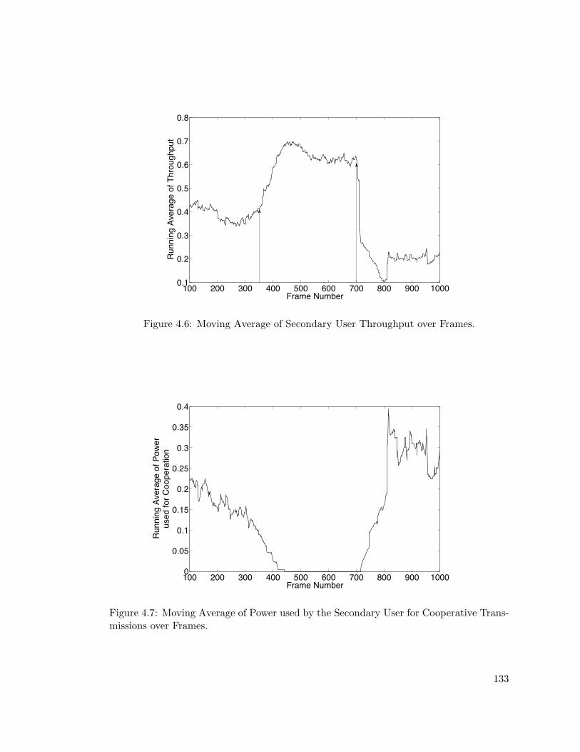
100 200 300 400 500 600 700 800 900 10000.1

0.2

0.3

0.4

0.5

0.6

0.7

0.8

Frame Number

Runn

ing

Aver

age

of T

hrou

ghpu

t

Figure 4.6: Moving Average of Secondary User Throughput over Frames.

100 200 300 400 500 600 700 800 900 10000

0.05

0.1

0.15

0.2

0.25

0.3

0.35

0.4

Frame Number

Runn

ing

Aver

age

of P

ower

used

for C

oope

ratio

n

Figure 4.7: Moving Average of Power used by the Secondary User for Cooperative Trans-missions over Frames.

133

Chapter 5

Optimal Routing with Mutual Information Accumulation

In this chapter, we investigate optimal routing and scheduling strategies for multi-hop

wireless networks with rateless codes. Rateless codes allow each node of the network to

accumulate mutual information with every packet transmission. This enables a significant

performance gain over conventional shortest path routing. Further, it also outperforms

cooperative communication techniques that are based on energy accumulation. How-

ever, it requires complex and combinatorial networking decisions concerning which nodes

participate in transmission, and which decode ordering to use. We formulate three prob-

lems of interest in this setting: (i) minimum delay routing, (ii) minimum energy routing

subject to delay constraint, and (iii) minimum delay broadcast. All of these are hard

combinatorial optimization problems and we make use of several structural properties

of the optimal solutions to simplify the problems and derive optimal greedy algorithms.

Although the reduced problems still have exponential complexity, unlike prior works on

such problems, our greedy algorithms are simple to use and do not require solving any

linear programs. Further, using the insight obtained from the optimal solution to a linear

network, we propose two simple heuristics that can be implemented in polynomial time

134

in a distributed fashion and compare them with the optimal solution. Simulations sug-

gest that both heuristics perform very close to the optimal solution over random network

topologies.

5.1 Introduction

Cooperative communication promises significant gains in the performance of wireless net-

works over traditional techniques that treat the network as comprised of point-to-point

links. Cooperative communication protocols exploit the broadcast nature of wireless

transmissions and offer spatial diversity gains by making use of multiple relays for coop-

erative transmissions. This can increase the reliability and reduce the energy cost of data

transmissions in wireless networks. See [KMY06] for a recent comprehensive survey.

Most prior work in the area of cooperative communication has investigated physi-

cal layer techniques such as orthogonal repetition coding/signaling [LTW04], distributed

beamforming [MBM07], distributed space-time codes [LW03], etc. All these techniques

perform energy accumulation from multiple transmissions to decode a packet. In energy

accumulation, a receiver can decode a packet when the total received energy from multiple

transmissions of that packet exceeds a certain threshold. An alternate approach of recent

interest is based on mutual information accumulation [MMYZ07] [DLMY08]. In this ap-

proach, a node accumulates mutual information for a packet from multiple transmissions

until it can be decoded successfully. This is shown to outperform energy accumulation

based schemes, particularly in the high SNR regime, in [MMYZ07] [DLMY08].

135

Such a scheme can be implemented in practice using rateless codes of which Fountain

and Raptor codes [Lub02,BLM02,Sho04] are two examples. In addition to allowing mu-

tual information accumulation, rateless codes provide further advantages over traditional

fixed rate schemes in the context of fading relay networks as discussed in [CM07] [LL09].

Unlike fixed rate code schemes in which knowledge of the current channel state informa-

tion (CSI) is required at the transmitters, rateless codes adapt to the channel conditions

without requiring CSI. This advantage becomes even more important in large networks

where the cost of CSI acquisition grows exponentially with the network size. However,

this introduces a deep memory in the system because mutual information accumulated

from potentially multiple transmissions in the past can be used to decode a packet.

In this chapter, we study three problems on optimal routing and scheduling over a

multi-hop wireless network using mutual information accumulation. Specifically, we first

consider a network with a single source-destination pair and n relay nodes. When a node

transmits, the other nodes accumulate mutual information at a rate that depends on

their incoming link capacity. All nodes operate under bandwidth and energy constraints

as described in detail in Sec. 2.2. We consider two problems in this setting. In the first

problem, the transmit power levels of the nodes are fixed and the objective is to transmit

a packet from the source to the destination in minimum delay (Sec. 5.3). In the second

problem, the transmit power levels are variable and the objective is to minimize the sum

total energy to deliver a packet to the destination subject to a delay constraint (Sec. 5.4).

In the third problem, we consider the network model with fixed transmit power levels

(similar to the first problem) and with a single source where the objective is to broadcast

136

a packet to all the other nodes in minimum delay (Sec. 5.5). All of these objectives are

important in a variety of networking scenarios.

Related problems of optimal routing in wireless networks with multi-receiver diversity

have been studied in [LT06,LDFK09,NU09,DFGV10] while problems of optimal cooper-

ative diversity routing and broadcasting are treated in [KAMZ07,SSH+10,DGG10,BK11]

and references therein. Although these formulations incorporate the broadcast nature of

wireless transmissions, they assume that the outcome of each transmission is a binary

success/failure. Further, any packet that cannot be successfully decoded in one trans-

mission is discarded. This is significantly different from the scenario considered in this

chapter where nodes can accumulate partial information about a packet from different

transmissions over time. This can be thought of as networking with “soft” information.

Prior work on accumulating partial information from multiple transmissions includes

the work in [DLMY08, CJL+05, ACGW04, MY04a, SMS07, MY05, YMMZ08]. Specifi-

cally, [CJL+05] considers the problem of minimum energy unicast routing in wireless

networks with energy accumulation and shows that it is an NP-complete problem. Sim-

ilar results are obtained for the problem of minimum energy accumulative broadcast

in [ACGW04, MY04a, SMS07]. A related problem of accumulative multicast is stud-

ied in [MY05]. Minimum energy unicast routing with energy accumulation only at the

destination is considered in [YMMZ08]. Also related to the notion of accumulating par-

tial information are the works on hydrid-ARQ techniques such as [CT01, ZV05]. The

work closest to ours is [DLMY08] which treats the minimum delay routing problem with

mutual information accumulation. Both [MY04a] [DLMY08] develop an LP based for-

mulation for their respective problems that involves solving a linear program for every

137

possible ordering of relay nodes over all subsets of relay nodes to derive the optimal so-

lution. Thus, for a network with n relay nodes, this exhaustive approach requires solving∑nm=1

(nm

)m! > n! linear programs.

The primary challenge associated with solving the problems addressed in this chapter

is their inherent combinatorial nature. Unlike traditional shortest path routing problems,

the cost of routing with mutual information accumulation depends not only on the set of

nodes in the routing path, but also their relative ordering in the transmission sequence,

making standard shortest path algorithms inapplicable. Therefore, we approach the prob-

lem differently. To derive the optimal transmission strategy for the first problem, we first

formulate an optimization problem in Sec. 5.3.2 that optimizes over all possible trans-

mission orderings over all subsets of relay nodes (similar to [MY04a] [DLMY08]). This

approach clearly has a very high complexity of O(n!). Then in Sec. 5.3.3, we prove a key

structural property of the optimal solution that allows us to simplify the problem and

derive a simple greedy algorithm that only needs to optimize over all subsets of nodes.

Further, it does not require solving any linear programs. Thus, it has a complexity of

O(2n). We derive a greedy algorithm of the same complexity for the second problem in

Sec. 5.4. We note that this complexity, while still exponential, is a significant improve-

ment over O(n!). For example, with n = 10, this requires 210 = 1024 runs of a simple

greedy algorithm as compared to 10! = 3628800 runs of an LP solver. Note that for small

networks, (say, n ≤ 10), it is reasonable to use our algorithm to exactly compute the

optimal solution. Further, for larger n it provides a feasible way to compute the optimal

solution as a benchmark when comparing against simpler heuristics.

138

For the minimum delay broadcast problem, we identify a similar structural property

of the optimal solution in Sec. 5.5 that allows us to simplify the problem and derive a

simple greedy algorithm. While this greedy algorithm still has a complexity of O(n!), it

does not require solving any linear programs and thus improves over the result in [MY04a]

that requires solving n! linear programs. In general, we expect all these problems to be

NP-complete based on the results in [CJL+05,ACGW04,MY04a,SMS07].

For the special case of a line network, we derive the optimal solution in Sec. 5.3.5. Fi-

nally, in Sec. 5.6, we propose two simple heuristics that can be implemented in polynomial

time in a distributed fashion and compare them with the optimal solution. Simulations

suggest that both heuristics perform quite close to the optimal solution over random

network topologies.

Before proceeding, we note that the techniques we apply to get these structural results

can also be applied to similar problems that use energy accumulation instead of mutual

information accumulation.

5.2 Network Model

The network model consists of a source s, destination d and n relays r1, r2, . . . , rn as shown

in Fig. 5.1. There are no time variations in the channel states. This models the scenario

where the coherence time of the channels is larger than any considered transmission time

of the encoded bits. In the first two problems, the source has a packet to be delivered to

the destination. In the third problem, the source packet must to delivered to all nodes in

the network.

139

s d

r1r2

r3

r4

C12

C2dCs1

C34

C4dCs3

Figure 5.1: Example network with source, destination and 4 relay nodes. When a nodetransmits, every other node that has not yet decoded the packet accumulates mutualinformation at a rate given by the capacity of the link between the transmitter and thatnode.

Each node i transmits at a fixed power spectral density (PSD) Pi (in units of joules/sec/Hz)

that is uniform across its transmission band. However, the transmission duration for a

node is variable and is a design parameter. The total available bandwidth is W Hz. A

node can transmit the packet only if it has fully decoded the packet. For this, it must

accumulate at least Imax bits of total mutual information.

All transmissions happen on orthogonal channels in time or frequency and at most

one node can transmit over a frequency channel at any given time. The channel gain

between nodes i and j is given by hij . We assume a frequency non-selective, flat-fading

model. Under this assumption, the minimum transmission time under the two orthogonal

schemes (where nodes transmit in orthogonal time vs. frequency channels) is the same. In

the following, we will focus on the case where transmissions are orthogonal in time. When

a node i transmits, every other node j that does not have the full packet yet, receives

mutual information at a rate that depends on the transmission capacity Cij (in units

140

of bits/sec/Hz) of link i − j. This transmission capacity itself depends on the transmit

power and channel gain. For example, for an AWGN channel, using Shannon’s formula,

this is given by Cij = log2

[1+ hijPi

N0

]where N0/2 is the PSD of the noise process. If node

i transmits for duration ∆ over bandwidth W , then node j accumulates ∆WCij bits of

information. In the following, we assume W = 1 for simplicity. We assume that each

transmitting node uses independently generated ideal rateless codes so that the mutual

information collected by a node from different transmissions add up. 1 A similar model

has been considered in [DLMY08].

5.3 Minimum Delay Routing

Under the modeling assumptions discussed in Sec. 5.2, the problem of routing a packet

from the source to the destination in minimum time consists of the following sub-problems:

• First, which subset of relay nodes should take part in forwarding the packet?

• Second, in what order should these nodes transmit?

• And third, what should be the transmission durations for these nodes?

We next discuss the transmission structure of a general policy under this model.

5.3.1 Timeslot and Transmission Structure

Consider any transmission strategy G for routing the packet to the destination in the

model described above. This includes the choice of the relay set, the transmission order

1We can incorporate the non-idealities of the rateless codes by multiplying Cij with a factor 1/(1 + ε)where ε ≥ 0 is the overhead.

141

s transmits

t0 t1 t2 t3 tk tk+1

W

stage 0 stage 1 stage 2 stage k

!0 !1 !2 !k

s transmits

1 transmits s tx 1 tx 2 tx ...... 1 tx 2 tx .... k tx

Figure 5.2: Example timeslot and transmission structure. In each stage, nodes that havealready decoded the full packet transmit on orthogonal channels in time.

for this set, and the transmission durations for each node in this set. Let R denote the

subset of relay nodes that take part in the routing process under strategy G. By this, we

mean that each node in R is able to decode the packet before the destination and then

transmits for a non-zero duration. There could be other nodes that are able to decode

the packet before the destination, but these do not take part in the forwarding process

and are therefore not included in the set R.

Let k = |R| be the size of this set. Also, let O be the ordering of nodes in R

that describes the sequence in which nodes in R successfully decode the packet under

strategy G. Without loss of generality, let the relay nodes in the ordering O be indexed

as 1, 2, 3, . . . , k. Also, let the source s be indexed as 0 and the destination d be indexed

as k + 1. Initially, only the source has the packet. Let t0 be the time when it starts its

transmission and let t1, t2, . . . , tk denote the times when relays 1, 2, . . . , k in the ordering

O accumulate enough mutual information to decode the packet. Also, let tk+1 be the time

when the destination decodes the packet. By definition, t0 ≤ t1 ≤ t2 ≤ . . . ≤ tk ≤ tk+1.

We say that the transmission occurs over k + 1 stages, where stage j, j ∈ 0, 1, 2, . . . , k

142

represents the interval [tj , tj+1]. The state of the network at any time is given by the

set of nodes that have the full packet and the mutual information accumulated so far at

all the other nodes. Note that in any stage j, the first j nodes in the ordering O and

the source have the fully decoded packet. Thus, any subset of these nodes (including

potentially all of them) may transmit during this stage. Then the time-slot structure for

the transmissions can be depicted as in Fig. 5.2. We note that unlike Chapter 3, here,

the timeslot structure is not fixed and is part of the optimization problem. Also note

that in each stage, the set of relays that have successfully decoded the packet increases

by one (we ignore those relays that are not part of the set R).

We are now ready to formulate the problem of minimum delay routing with mutual

information accumulation.

5.3.2 Problem Formulation

For each j, define the duration of stage j as ∆j = tj+1 − tj . Also, let Aij denote the

transmission duration for node i in stage j under strategy G. Note that Aij = 0 if

i > j, else Aij ≥ 0. This is because node i does not have the full packet until the end

of stage i − 1. The total time to deliver the packet to the destination Ttot is given by

Ttot = tk+1− t0 =∑k

j=0 ∆j . For any transmission strategy G that uses the subset of relay

nodes R with an ordering O, the minimum delay is given by the solution to the following

optimization problem:

143

Minimize: Ttot =k∑j=0

∆j

Subject to:m−1∑i=0

m−1∑j=0

AijCim ≥ Imax ∀m ∈ 1, 2, . . . , k + 1

j∑i=0

Aij ≤ ∆j ∀j ∈ 0, 1, 2, . . . , k

Aij ≥ 0 ∀i ∈ 0, 1, 2, . . . , k, j ∈ 0, 1, 2, . . . , k

Aij = 0 ∀i > j

∆j ≥ 0 ∀j ∈ 0, 1, 2, . . . , k (5.1)

Here, the first constraint captures the requirement that node m in the ordering must

accumulate at least Imax amount of mutual information by the end of stage m− 1 using

all transmissions in all stages up to stage m − 1. The second constraint means that in

every stage j, the total transmission time for all nodes that have the fully decoded packet

in that stage cannot exceed the length of that stage. We note that the solution to (5.1)

may result in a decoding order that is different from O. In that case, the decoding order

O is infeasible. It can be seen that the above problem is a linear program and thus can be

solved efficiently for a given relay set R and its ordering O. Indeed, this is the approach

taken in [DLMY08] that proposes solving such a linear program for every possible ordering

of relays for each subset of the set of relay nodes. While such an approach is guaranteed

to find the optimal solution, it has a huge computational complexity of O(n!) linear

programs. In the next section, we show that the above computation can be significantly

simplified by making use of a key structural property of the optimal solution.

144

s transmits1 gets the

packet,1 transmits

2 gets the packet,

2 transmits

k gets the packet,

k transmits

t0 t1 t2 t3 tk tk+1

W .......

stage 0 stage 1 stage 2 stage k

!0 !1 !2 !k

Figure 5.3: Optimal timeslot and transmission structure. In each stage, only the nodethat decodes the packet at the beginning of that stage transmits.

5.3.3 Characterizing the Optimal Solution of (5.1)

Let Ropt denote the subset of relay nodes that take part in the routing process in the

optimal solution. Let k = |Ropt| be the size of this set. Also, let Oopt be the optimal

ordering. Note that, by definition, each node in Ropt transmits for a non-zero duration

(else, we can remove it from the set without affecting the minimum total transmission

time). Then, we have the following:

Theorem 6 Under the optimal solution to the minimum delay routing problem (5.1), in

each stage j, it is optimal for only one node to transmit, and that node is node j.

Fig. 5.3 shows the timeslot structure under the optimal solution. The above theorem

shows that only one node transmits in each stage, and that the optimal transmission

ordering is the same as the ordering that nodes in the set Ropt decode the packet. Com-

paring this with the general timeslot structure in Fig. 5.2, it can be seen that Theorem 6

simplifies problem (5.1) significantly. Specifically, Theorem 6 implies that, given the op-

timal relay set Ropt, the optimal transmission structure (i.e., the decoding order and the

transmission durations) can be computed in a greedy fashion as follows. First, the source

145

starts to transmit and continues to do so until any relay node in this set gets the packet.

Once this relay node gets the packet, we know from Theorem 6 that the source does not

transmit in any of the remaining stages. This node then starts to transmit until another

node in the set gets the packet. This process continues until the destination is able to

decode the packet. The optimal solution to (5.1) can then be obtained by applying this

greedy transmission strategy to all subsets of relay nodes and picking one that yields the

minimum delay.2 Note that applying this greedy transmission strategy does not require

solving an LP. While searching over all subsets still has an exponential complexity of

O(2n), it can be used to compute the optimal solution as a benchmark. Theorem 6 also

implies that multiple copies of the packet need not be maintained across the network.

For example, note that the source need not transmit after the first relay has decoded the

packet and therefore can drop the packet from its queue.

We emphasize that the optimal transmission structure suggested by Theorem 6 is not

obvious. For example, at the beginning of any stage, the newest addition to the set of

relay nodes with the full packet may not have the best links (in terms of transmission

capacity) to all the remaining nodes, including the destination. This would suggest that

under the optimal solution, in general in each stage, nodes with the full packet should

take turns transmitting the packet. However, Theorem 6 states that such time-sharing is

not required.

Before proceeding, we present a preliminary Lemma that is used in the proof of

Theorem 6. Consider any linear program:

2We note that the transmission structure characterized by Theorem 6 is similar to the wavepath propertyshown in [CJL+05] for the problem of minimum energy unicast routing with energy accumulation inwireless networks. However, our proof technique is significantly different.

146

Minimize: cTx

Subject to: Ax = b

x ≥ 0 (5.2)

where x ∈ Rn. Then we have the following:

Lemma 4 Let x∗ be an optimal solution to the problem (5.2) such that x∗ > 0 (where the

inequality is taken entry wise). Then x∗ is still an optimal solution when the constraint

x ≥ 0 is removed.

Lemma 4 implies that removing an inactive constraint does not affect the optimal

solution of the linear program. This is a simple fact and its proof is provided for com-

pleteness in Appendix D.1.

5.3.4 Proof of Theorem 6

Note that Theorem 6 trivially holds in stage 0 (since only the source has the full packet

in this stage). Next, it is easy to see that in the last stage (i.e., stage k), only the node

with the best link (in terms of transmission capacity) to the destination in the set Ropt

should transmit in order to minimize the total delay. This is because this node will take

the smallest time to transmit the remaining amount of mutual information needed by d

to decode the packet. Further, we claim that this node must be the node k in the ordering

Oopt. This can be argued as follows. Assume that the node with the best link to the

destination in the set Ropt has the full packet at some stage (k − j) (where 0 < j < k)

147

before the start of stage k. Then a smaller delay can be achieved by having only this node

transmit after it has decoded the full packet from that stage onwards. Thus, the other

nodes labeled k− j, . . . , k− 1 in the transmission order do not transmit, a contradiction.

This shows that under the optimal solution, in the last stage k, only node k in the ordering

Oopt transmits. Using induction, we now show that in every prior stage (k − j) where

1 ≤ j ≤ k − 1, only one node needs to transmit and that this node must be node k − j

in the ordering Oopt.

Consider the (k − 1)th stage. At time tk−1, all nodes except k and d have decoded

the packet. Let the mutual information state at nodes k and d at time tk−1 be Ik(tk−1)

and Id(tk−1) respectively. Also, suppose in the (k− 1)th stage, relay nodes 1, 2, . . . , k− 1

and the source transmit a fraction αk−11 , αk−1

2 , . . . , αk−1k−1 and αk−1

0 of the total duration

of stage (k − 1), i.e., ∆k−1 respectively. Note that these fractions must add to 1 since it

is suboptimal to have any idle time (where no one is transmitting). Then, the optimal

solution must solve the following optimization problem:

Minimize: ∆k−1 + ∆k

Subject to: Ik(tk−1) + ∆k−1

k−1∑i=0

αk−1i Cik ≥ Imax

Id(tk−1) + ∆k−1

k−1∑i=0

αk−1i Cid + ∆kCkd ≥ Imax

0 ≤ αk−10 , αk−1

1 , . . . , αk−1k−1 ≤ 1

k−1∑i=0

αk−1i = 1

∆k−1 ≥ 0,∆k ≥ 0 (5.3)

148

Here, the first constraint states that relay k must accumulate at least Imax bits of mutual

information by the end of stage (k−1). The second constraint states that the destination

must accumulate at least Imax bits of mutual information by the end of stage k. Note

that in the last term of the left hand side of the second constraint, we have used the fact

that only node k transmits during stage k.

It is easy to see that under the optimal solution, the first and second constraints must

be met with equality. This simply follows from the definition of the beginning of any

stage j as the time when node j has just decoded the packet. Next, let βi = ∆k−1αk−1i

for all i ∈ 0, 1, 2, . . . , k − 1. Since∑k−1

i=0 αk−1i = 1, we have that

∑k−1i=0 βi = ∆k−1 and

(5.3) is equivalent to:

Minimize:k−1∑i=0

βi + ∆k

Subject to: Ik(tk−1) +k−1∑i=0

βiCik = Imax

Id(tk−1) +k−1∑i=0

βiCid + ∆kCkd = Imax

∆k ≥ 0, βi ≥ 0 ∀i ∈ 0, 1, 2, . . . , k − 1 (5.4)

Note that problems (5.3) and (5.4) are equivalent because we can transform (5.4) to

the original problem by using the relations ∆k−1 =∑k−1

i=0 βi and αk−1i = βi

∆k−1. The

degenerate case where ∆k−1 = 0 does not arise because if ∆k−1 = 0, then no node

transmits in stage (k − 1) and we transition to stage k in which only node k transmits.

149

This means node k−1 never transmits, contradicting the fact that it is part of the optimal

transmission schedule.

Since we know that under the optimal solution, ∆k > 0, we can remove the constraint

∆k ≥ 0 from (5.4) without affecting the optimal solution (using Lemma 4). Next we

multiply the minimization objective in (5.4) by Ckd without changing the problem. Then,

using the second equality constraint to eliminate ∆k from the objective and ignoring the

constant terms, (5.4) can be expressed as:

Minimize:k−1∑i=0

βi(Ckd − Cid)

Subject to: Ik(tk−1) +k−1∑i=0

βiCik = Imax

βi ≥ 0 ∀i ∈ 0, 1, 2, . . . , k − 1 (5.5)

This optimization problem is linear in βi with a single linear equality constraint and thus

the solution is of the form where all except one βi are zero. Since αk−1i = βi

∆k−1, we have

that in the optimal solution, exactly one of the fractions αk−10 , αk−1

1 , . . . , αk−1k−1 is equal to

1 and rest must be 0. This implies that only one node transmits in this stage. Further,

this node must be the relay node k − 1 that decoded the packet at the beginning of this

stage. Else, node k − 1 never transmits. This is because by definition of stage (k − 1),

node k−1 does not have the packet before the beginning of stage (k−1) and hence cannot

transmit before stage (k − 1). Since only node k transmits when stage (k − 1) ends, if

150

node k − 1 is not the node chosen for stage (k − 1), it never transmits, contradicting the

fact that it is part of the optimal set.3

Now consider the (k−j)th stage and suppose Theorem 6 holds for all stages after stage

(k−j) where 2 ≤ j ≤ k−1. This means that in every stage after stage (k−j), only the node

that has just decoded the packet transmits. At time tk−j , all nodes except k−j+1, k−j+

2, . . . , k and d have decoded the packet. Let the mutual information state at these nodes

at time tk−j be Ik−j+1(tk−j), Ik−j+2(tk−j), . . . , Ik(tk−j) and Id(tk−j), respectively. Also,

suppose in the (k − j)th stage, the source and the relay nodes 1, 2, . . . , k − j transmit

a fraction αk−j0 , αk−j1 , αk−j2 , . . . , αk−jk−j of the total duration of stage (k − j), i.e., ∆k−j

respectively. Then, the optimal solution must solve the following optimization problem:

Minimize:j∑

m=0

∆k−j+m

Subject to: Ik−j+1(tk−j) + ∆k−j

[ k−j∑i=0

αk−ji Ci,k−j+1

]= Imax

Ik−j+n(tk−j) + ∆k−j

[ k−j∑i=0

αk−ji Ci,k−j+n

]+

n−1∑i=1

∆k−j+iCk−j+i,k−j+n = Imax ∀n ∈ 2, . . . , j + 1

0 ≤ αk−j0 , αk−j1 , . . . , αk−jk−j ≤ 1

k−j∑i=0

αk−ji = 1

∆k−j ≥ 0,∆k−j+1 ≥ 0, . . . ,∆k ≥ 0 (5.6)

3This is a crucial property that holds only for the unicast routing case. As we will see in Sec. 5.5, thisdoes not necessarily hold for the minimum delay broadcast problem.

151

where the first constraint states that relay k− j+ 1 must accumulate Imax bits of mutual

information by the end of stage (k − j). The second set of constraints state that every

subsequent node k− j+n (where 2 ≤ n ≤ j+1) including the destination in the ordering

Oopt must accumulate Imax bits of mutual information by the end of stage (k − j + n).

In the last term of the left hand side of each such constraint, we have used the induction

hypothesis that in every stage after stage (k − j), only the node that just decoded the

packet transmits. Using the transform βi = ∆k−jαk−ji for all i ∈ 0, 1, 2, . . . , k − j, and∑k−j

i=0 αk−ji = 1, we have the equivalent problem:

Minimize:k−j∑i=0

βi + ∆k−j+1 + . . .+ ∆k−1 + ∆k

Subject to: Ik−j+1(tk−j) +k−j∑i=0

βiCi,k−j+1 = Imax

Ik−j+n(tk−j) +k−j∑i=0

βiCi,k−j+n+

n−1∑i=1

∆k−j+iCk−j+i,k−j+n = Imax ∀n ∈ 2, . . . , j + 1

βi ≥ 0 ∀i ∈ 0, 1, 2, . . . , k − j

∆k−j+1 ≥ 0, . . . ,∆k ≥ 0 (5.7)

The problems (5.6) and (5.7) are equivalent because we can transform (5.7) to the

original problem by using the relations ∆k−j =∑k−j

i=0 βi and αk−ji = βi∆k−j

. The degen-

erate case where ∆k−j = 0 does not arise because if ∆k−j = 0, then no node transmits

in stage (k − j). We know from the induction hypothesis that only the nodes after node

152

k− j in the ordering Oopt transmit after stage (k− j). This means that node k− j never

transmits, a contradiction.

The second set of constraints in problem (5.7) can be written in matrix form as

B + C∆ = I as shown below.

∑k−ji=0 βiCi,k−j+2∑k−ji=0 βiCi,k−j+3

...∑k−ji=0 βiCi,d

+

Ck−j+1,k−j+2 . . . 0

Ck−j+1,k−j+3 . . . 0

.... . .

...

Ck−j+1,d . . . Ck,d

∆k−j+1

∆k−j+2

...

∆k

=

Imax − Ik−j+2(tk−j)

Imax − Ik−j+3(tk−j)

...

Imax − Id(tk−j)

From this, we note that C is a lower triangular matrix. Thus, we have: ∆ = C−1(I−

B). Therefore each of the terms ∆k−j+1,∆k−j+2, . . . ,∆k−1,∆k is linear in the variables

β0, β1, . . . , βk−j . Using this, the objective in (5.7) can be expressed as a linear function

of these variables. Let this be denoted by f(β0, β1, . . . , βk−j). Also we know that under

the optimal solution, ∆k−j+1 > 0, . . . ,∆k > 0. Thus, we can remove the last set of

constraints from (5.7) without affecting the optimal solution (using Lemma 4). Thus,

(5.7) becomes:

Minimize: f(β0, β1, . . . , βk−j)

Subject to: Ik−j+1(tk−j) +k−j∑i=0

βiCi,k−j+1 = Imax

βi ≥ 0 ∀i ∈ 0, 1, 2, . . . , k − j (5.8)

153

s 1 2 3 dnmm+1

Figure 5.4: A line network.

Similar to the stage (k − 1) case, this optimization problem is linear in βi with a single

linear equality constraint and thus the solution is of the form where all except one βi

are zero. Since αk−ji = βi∆k−j

, we have that in the optimal solution, exactly one of the

fractions αk−j0 , αk−j1 , . . . , αk−jk−j is equal to 1 and rest must be 0. This implies that only

one node transmits in this stage. Further, this node must be the relay node k − j that

decoded the packet at the beginning of this stage. Else, node k− j never transmits. This

is because by definition of stage (k − j), node k − j does not have the packet before the

beginning of stage (k − j) and hence cannot transmit before stage (k − j). By induction

hypothesis, only nodes k− j+ 1, k− j+ 2, . . . , k transmit when stage (k− j) ends. Thus,

if node k − j is not the node chosen for stage (k − j), it never transmits, contradicting

the fact that it is part of the optimal set. This proves the Theorem.

5.3.5 Exact Solution for a Line Network

In this section, we present the optimal solution for a special case of line networks. Specif-

ically, all nodes are located on a line as shown in Fig. 5.4. We assume that each node

transmits at the same PSD P . Further, the transmission capacity Cij between any two

nodes i and j depends only on the distance dij between the two nodes and is a monotoni-

cally decreasing function of dij . For example, we may have that Cij = log(1+ hijPN0

) where

154

P is the PSD and hij = 1dαij

where α ≥ 2 is the path loss coefficient. Under these assump-

tions, the following Lemma characterizes the optimal cooperating set for the problem of

routing with mutual information accumulation. Its proof is provided in Appendix D.2.

Lemma 5 The optimal cooperating set for the line network as described above is given

by the set of all relay nodes located between the source and the destination.

To get an idea of the reduction in delay achieved by using mutual information accu-

mulation over traditional routing, consider the line network example above with n nodes

placed between s and d at equal distance such that di,i+1 = 1 for all i. Also, suppose

the transmission capacity on link i − j is given by Cij = γPd2ij

where γ > 0 is a constant.

Then the capacity of link s− 1 is γP , the capacity of link s− 2 is γP4 , the capacity of link

s− 3 is γP9 , and so on. Define θM=γP . Then, the minimum delay for routing with mutual

information accumulation is given by∑n

i=0 ∆i where:

∆0 =ImaxCs1

=Imaxθ

,∆1 =Imax −∆0Cs2

C12=Imax −∆0

θ4

θ

...

∆n =Imax −

∑n−1i=0 ∆iCi,n+1

Cn,n+1=Imax −

∑n−1i=0 ∆i

θ(n+1−i)2

θ

For simplicity, let us ignore the contribution of nodes that are more than 3 units away

from a receiver. Then, we have:

155

n∑i=0

∆i =(n+ 1)Imax − θ

4

∑n−1i=0 ∆i − θ

9

∑n−2i=0 ∆i

θ

⇒n∑i=0

∆i =(n+ 1)Imax + θ

4∆n + θ9(∆n + ∆n−1)

θ(1 + 14 + 1

9)<

(n+ 1)Imax + θ4∆0 + θ

92∆0

θ(1 + 14 + 1

9)

=Imaxθ

(n+ 1 + 1

4 + 29

1 + 14 + 1

9

)

where we used the fact that ∆n,∆n−1 < ∆0. The minimum delay for traditional routing

is simply (n + 1)∆0 = (n + 1) Imaxθ . Thus, for this network, the delay under mutual

information accumulation is smaller than that under traditional routing at least by a

factor n+1+ 14

+ 29

(n+1)(1+ 14

+ 19

)that approaches 36

49 = 73% for large n.

5.4 Minimum Energy Routing with Delay Constraint

Next, we consider the second problem of minimizing the sum total energy to transmit

a packet from the source to destination using mutual information accumulation subject

to a given delay constraint Dmax. This problem is more challenging than problem (5.1)

since in addition to optimizing over the cooperating relay set and the order of transmis-

sion, it also involves determining the PSD values to be used for each node. Further, a

cooperating relay node may need to transmit at different PSD levels in different stages

of the transmission schedule.

156

5.4.1 Problem Formulation

Consider a transmission strategy (similar to the one discussed in Sec. 5.3.1) that is

described by a cooperating relay set R of size |R| = k and a decoding order O. Let the

terms ∆j and Aij be defined in a similar fashion. Also, let Pij denote the PSD at which

node i transmits in stage j. Then for any transmission strategy G that uses the subset of

relay nodes R with an ordering O, the minimum sum total energy to transmit a packet

from source to destination subject to the delay constraint Dmax is given by the solution

to the following optimization problem:

Minimize:k∑j=0

j∑i=0

AijPij

Subject to:k∑j=0

∆j ≤ Dmax

m−1∑i=0

m−1∑j=0

AijCim(Pij) ≥ Imax ∀m ∈ 1, . . . , k + 1

j∑i=0

Aij ≤ ∆j ∀j ∈ 0, 1, 2, . . . , k

Aij , Pij ≥ 0 ∀i ∈ 0, 1, 2, . . . , k, j ∈ 0, 1, . . . , k

Aij = 0, Pij = 0 ∀i > j, ∆j ≥ 0 ∀j ∈ 0, 1, 2, . . . , k (5.9)

where the first constraint represents requirement that the total delay must not exceed

Dmax. The second constraint captures the requirement that node m in the ordering must

accumulate at least Imax amount of mutual information by the end of stage m−1 using all

transmissions in all stages up to stage m− 1. In the second constraint, Cim(Pij) denotes

157

the transmission capacity of link i−m in stage j and it is a function of Pij , the PSD of

node i in stage j. Note that (5.9) is not a linear program in general, since the Cim(Pij)

may be non-linear in Pij . Also note that the solution to (5.9) may result in a decoding

order that is different from O in which case that decoding order is infeasible.

5.4.2 Characterizing the Optimal Solution of (5.9)

Let Ropt denote the subset of relay nodes that take part in the routing process in the

optimal solution. Let k = |Ropt| be the size of this set. Also, let Oopt be the optimal

ordering. Note that, by definition, each node in Ropt transmits for a non-zero duration

(else, we can remove it from the set without affecting the sum total energy). Finally, let

P optij denote the optimal PSD used by node i in stage j. Then, similar to Theorem 6, we

have the following:

Theorem 7 Under the optimal solution to the minimum sum total energy subject to delay

constraint problem (5.9), in each stage j, it is optimal for only one node to transmit, and

that node is node j.

Proof 6 The proof is similar to the proof of Theorem 6 and is omitted for brevity.

Although Theorem 7 simplifies the optimization problem (5.9), it cannot be solved

using the greedy transmission strategy applied over all subsets as discussed in Sec. 5.3.3.

This is because the transmission order generated by the greedy strategy depends on the

power levels used. For general non-linear rate-power functions, different power levels can

give rise to different decoding orders for the same relay set under the greedy strategy

(see Appendix D.3 for an example). Thus, solving (5.9) may involve searching over all

158

possible orderings of all possible subsets. However, for the special, yet important case of

linear rate-power functions, this problem can be simplified considerably. A linear rate-

power function is a good approximation for the low SNR regime. For example, in sensor

networks where bandwidth is plentiful and power levels are small, it is reasonable to

assume that the nodes operate in the low SNR regime. In the following, we will assume

that the transmission capacity Cij(Pi) on link i− j is given by Cij(Pij) = γPihij (in units

of bits/sec/Hz) where γ is a constant and Pi is the PSD of node i. Then, we have the

following:

Theorem 8 For linear rate-power functions, the decoding order of nodes in the optimal

set Ropt under the greedy transmission strategy is the same for all non-zero power alloca-

tions. Further, the sum total power required to transmit a packet from the source to the

destination is the same for all non-zero power allocations.

Proof 7 We prove by induction. Consider any non-zero power allocation used by the

nodes in Ropt. The source is the first node to transmit. Let it be indexed by 0. Also,

suppose the source uses PSD P0 > 0. Under the greedy transmission strategy, the source

continues to transmit until any node can decode the packet. This node is the one that

minimizes ∆0 = ImaxC0i(P0) = Imax

γP0h0iover all i ∈ Ropt, which is the time to decode the packet.

Clearly, this node is the same for all P0 > 0. Let it be indexed by 1. Also, we have that:

∆0 =ImaxγP0h01

⇒ ∆0P0 =Imaxγh01

159

which shows that the total power used in stage 0 is independent of P0. Next, let the PSD

of node 1 be P1. Then, in stage 1 under the greedy transmission strategy, node 1 transmits

until any node that does not have the packet yet can decode it. This node is the one that

minimizes over all i ∈ Ropt \ 1:

Imax −∆0C0i(P0)C1i

=Imax −∆0γP0h0i

γP1h1i=Imax(1− h0i

h01)

γP1h1i

Clearly, this node is the same for all P1 > 0. Let it be indexed by 2. Also, we have that:

∆1 =Imax(1− h02

h01)

γP1h12⇒ ∆1P1 =

Imax(1− h02)γh01

γh12

which shows that the total power used in stage 1 is independent of P0 and P1.

Now suppose this holds for all stages 0, 1, 2, . . . , j − 1 where j − 1 < k. We show

that it also holds for stage j. Let the PSD of node j be Pj. Under the greedy strategy,

node j continues to transmit in stage j until any node that does not have the packet yet

can decode it. This node is the one that minimizes over all i ∈ Ropt \ 1, 2, . . . , j:

Imax −∑j−1

m=0 ∆mCmi(Pm)Cji(Pj)

=Imax − γ

∑j−1m=0 ∆mPmhmi

γPjhji

From the induction hypothesis, we know that each of the terms ∆mPm for all m ∈

0, 1, . . . , j − 1 is independent of the power levels Pm. Thus, we have that the node

160

that minimizes the expression above is the same for all Pj > 0. Further, the total power

used in stage j is given by

∆jPj =Imax − γ

∑j−1m=0 ∆mPmhmiγhji

which is independent of P0, P1, . . . , Pm. This proves the Theorem.

5.4.3 A Greedy Algorithm

Theorem 8 suggests a simple method for computing the optimal solution to (5.9) when the

rate-power function is linear. Specifically, we start by setting all PSD levels to the same

value, say some P > 0. From Theorem 8, we know that the sum total power required to

transmit a packet from the source to the destination is the same for all non-zero power

allocations. Then, solving (5.9) is equivalent to solving the minimum delay problem (5.1)

with given power levels, except the delay constraint. This can be done using the greedy

strategy described in Sec. 5.3.3. If the solution obtained satisfies the delay constraint

Dmax, then we are done. Else, suppose we get a delay D > Dmax. Then, we can scale

up the power level P by a factor DDmax

and scale down the duration of each stage ∆j by

the same factor. This ensures that the delay constraint is met while the sum total power

used remains the same.

161

5.5 Minimum Delay Broadcast

Next, we consider the problem of minimum delay broadcast for the network model de-

scribed in Sec. 5.2. In this problem, starting with the source node, the goal is to deliver

the packet to all nodes in the network in minimum time with mutual information accumu-

lation. We assume that there are n nodes in the network other than the source. Similar

problems have been considered in [ACGW04,MY04a,SMS07] which focus on energy ac-

cumulation and where the goal is to broadcast the packet to all nodes using minimum

sum total energy.

5.5.1 Timeslot and Transmission Structure

For the minimum delay broadcast problem, the transmission strategy and resulting time

timeslot structure under a general policy is similar to the one discussed for the minimum

delay routing problem in Sec. 5.3.1. Specifically, let O be the ordering of the n nodes

that represents the sequence in which they successfully decode the packet under a given

strategy. Without loss of generality, let the nodes in the ordering O be indexed as

1, 2, 3, . . . , n. Also, let the source s be indexed as 0. Initially, only the source has the

packet. Let t0 be the time when it starts its transmission and let t1, t2, . . . , tn denote the

times when nodes 1, 2, . . . , n in the ordering O accumulate enough mutual information

to decode the packet. We say that the transmission occurs over n stages, where stage

j, j ∈ 0, 1, 2, . . . , n − 1 represents the interval [tj , tj+1]. Note that in any stage j, the

first j nodes in the ordering O and the source have the fully decoded packet. Thus,

any subset of these nodes (including potentially all of them) may transmit during this

162

stage. For each j, define the duration of stage j as ∆j = tj+1 − tj . Also, let Aij denote

the transmission duration for node i in stage j. As before, we have that Aij = 0 if

i > j, else Aij ≥ 0. The total time to deliver the packet to all the n nodes is given by

Ttot = tn − t0 =∑n−1

j=0 ∆j .

5.5.2 Problem Formulation

For any transmission strategy that results in the decoding order O, the minimum delay

for broadcast is given by the solution to the following optimization problem:

Minimize: Ttot =n−1∑j=0

∆j

Subject to:m−1∑i=0

m−1∑j=0

AijCim ≥ Imax ∀m ∈ 1, 2, . . . , n

j∑i=0

Aij ≤ ∆j ∀j ∈ 0, 1, 2, . . . , n− 1

Aij ≥ 0 ∀i ∈ 0, 1, 2, . . . , n− 1, j ∈ 0, 1, 2, . . . , n− 1

Aij = 0 ∀i > j

∆j ≥ 0 ∀j ∈ 0, 1, 2, . . . , n− 1 (5.10)

This is similar to (5.1) except that the set R contains all n nodes and that d is not

necessarily the last node to decode the packet. Similar to (5.1), the first constraint

captures the requirement that node m in the decoding order O must accumulate at least

Imax amount of mutual information by the end of stage m− 1 using transmissions in all

stages up to stage m − 1. The second constraint means that in every stage j, the total

transmission time for all nodes that have the fully decoded packet in that stage cannot

163

exceed the length of that stage. We note that the solution to (5.10) may result in a

decoding order that is different from O. In that case, the decoding order O is infeasible.

Similar to (5.1), the above problem is a linear program and thus can be solved ef-

ficiently for a given ordering O. This is the approach taken in [MY04a] (with energy

accumulation instead of mutual information accumulation, and with the objective of

minimizing total energy for broadcast instead of delay) that proposes solving such a lin-

ear program for every possible ordering of the n nodes, resulting in n! linear programs.

In the next section, we show that the above computation can be simplified by making use

of a structural property of the optimal solution that is similar to the results of Theorems

6 and 7. This results in a greedy algorithm that does not require solving such linear

programs to compute the optimal solution.

5.5.3 Characterizing the Optimal Solution of (5.10)

Let Oopt be the decoding order under the optimal solution. Suppose the the nodes in the

ordering are labeled as 0, 1, 2, . . . , n− 1, n with 0 being the source node. Then, similar

to Theorems 6 and 7, we have the following:

Theorem 9 Under the optimal solution to the minimum delay broadcast problem (5.10),

in each stage j, it is optimal for at most one node to transmit.

While Theorem 9 states that under the optimal solution, at most one node transmits

in each stage j, unlike Theorems 6 and 7, it does not say that this node must be node j.

In fact, this node could be any one of the nodes that have the full packet. Let rj be the

node that transmits in stage j. Then, using Theorem 9, we have that rj ∈ 0, 1, 2, . . . , j.

164

s transmits

1 gets thepacket,

r1 transmits,r1! s, 1

2 gets thepacket,

r2 transmits,r2 ! s, 1, 2

n-1 gets thepacket,

rn-1 transmits,rn-1! s, 1,..., n-1

t0 t1 t2 t3 tn-1 tn

W .......

stage 0 stage 1 stage 2 stage n-1

!0 !1 !2 !n-1

Figure 5.5: Optimal timeslot and transmission structure for minimum delay broadcast.In each stage, at most one node from the set of nodes that have the full packet transmits.

The optimal timeslot structure for the minimum delay broadcast problem is shown in

Fig. 5.5. Note that unlike Fig. 5.3, here it is possible for a node to transmit more than

once over the course of the broadcast.

This property does not reduce the complexity of finding the optimal solution from

O(n!) linear programs to O(2n). However, as we show in Sec. 5.5.5, it still leads to

a greedy algorithm to find the optimal solution that does not require solving n! linear

programs like [MY04a].

5.5.4 Proof of Theorem 9

The proof is similar to the proof of Theorem 6 and therefore, we only provide a sketch

here, highlighting the main differences.

Note that Theorem 9 trivially holds in stage 0 (since only the source has the full

packet in this stage). Next, similar to Theorem 6, in the last stage (i.e., stage (n − 1)),

only the node with the best link (in terms of transmission capacity) to node n in the

ordering Oopt should transmit in order to minimize the total delay. Let this node be

165

labeled rn−1. However, unlike Theorem 6, we cannot claim that this node must be node

n− 1 in the ordering Oopt. This is because while rn−1 has the best link to n, it does not

necessarily have the best links to all those nodes in the decoding order Oopt that come

after rn−1. Thus rn−1 could be any one of 0, 1, 2, . . . , n− 1. This shows that under the

optimal solution, in the last stage (n−1), only one node rn−1 transmits. Using induction,

we can show that in every prior stage (n− j) where 1 < j < n, at most one node needs

to transmit.

Consider the (n−2)th stage. At time tn−2, all nodes except n−1 and n have decoded

the packet. Let the mutual information state at nodes n − 1 and n at time tn−2 be

In−1(tn−2) and In(tn−2) respectively. Also, suppose in the (n − 2)th stage, relay nodes

1, 2, . . . , n − 2 and the source transmit a fraction αn−21 , αn−2

2 , . . . , αn−2n−2 and αn−2

0 of the

total duration of stage (n − 2), i.e., ∆n−2, respectively. Note that these fractions must

add to 1 since it is suboptimal to have any idle time (where no one is transmitting).

Then, the optimal solution must solve the following optimization problem:

Minimize: ∆n−2 + ∆n−1

Subject to: In−1(tn−2) + ∆n−2

n−2∑i=0

αn−2i Ci,n−1 ≥ Imax

In(tn−2) + ∆n−2

n−2∑i=0

αn−2i Cin + ∆n−1Crn−1,n ≥ Imax

0 ≤ αn−20 , αn−2

1 , . . . , αn−2n−2 ≤ 1

n−2∑i=0

αn−2i = 1

∆n−2 ≥ 0,∆n−1 ≥ 0 (5.11)

166

Here, the first constraint states that node n − 1 must accumulate at least Imax bits of

mutual information by the end of stage (n− 2). The second constraint states that node

n must accumulate at least Imax bits of mutual information by the end of stage (n− 1).

Note that in the last term of the left hand side of the second constraint, we have used

the fact that only node rn−1 transmits during stage (n− 1).

It is easy to see that under the optimal solution, the first and second constraints must

be met with equality. This simply follows from the definition of the beginning of any

stage j as the time when node j has just decoded the packet. Next, let βi = ∆n−2αn−2i

for all i ∈ 0, 1, 2, . . . , n− 2. Since∑n−2

i=0 αn−2i = 1, we have that

∑n−2i=0 βi = ∆n−2 and

(5.11) is equivalent to:

Minimize:n−2∑i=0

βi + ∆n−1

Subject to: In−1(tn−2) +n−2∑i=0

βiCi,n−1 = Imax

In(tn−2) +n−2∑i=0

βiCin + ∆n−1Crn−1,n = Imax

∆n−1 ≥ 0, βi ≥ 0 ∀i ∈ 0, 1, 2, . . . , n− 2 (5.12)

Note that problems (5.11) and (5.12) are equivalent because we can transform (5.12)

to the original problem by using the relations ∆n−2 =∑n−2

i=0 βi and αn−2i = βi

∆n−2. In the

degenerate case where ∆n−2 = 0, we have that no node transmits in stage (n − 2), so

that Theorem 9 holds.

Using similar arguments as in Theorem 6, it can be shown that when ∆n−2 > 0, then

in the optimal solution exactly one of the fractions αn−20 , αn−2

1 , . . . , αn−2n−2 is equal to 1 and

167

rest must be 0. This implies that only one node transmits in this stage. Combining with

the case where ∆n−2 = 0, we have that at most one node transmits in stage (n− 2). We

label this node as rn−2. Note that rn−2 could be any one of 0, 1, 2, . . . , n− 2.

Using induction, it can be shown that in every stage (n− j), 2 < j < n, at most one

node labeled rn−j transmits. Further, rn−j could be any one of 0, 1, 2, . . . , n− j. This

proves the Theorem.

5.5.5 A Greedy Algorithm

Theorem 9 can be used to construct the following greedy algorithm for computing the

optimal solution to (5.10). The algorithm operates over n stages. In each stage j,

0 ≤ j ≤ n − 1, the algorithm performs (j + 1)! separate runs as discussed below. Let

Sij denote the set of nodes that have the full packet at the end of the ith run of stage

j. Then, each run in stage j + 1 corresponds to selecting one transmitter from each Sij

and having that node transmit until a new node decodes the packet. Thus, the number

of nodes with the full packet increases by one at the end of each run. We will show that

the size of Sij is equal to ‖Sij‖ = j+ 2 for all i, j. Further, there are (j+ 1)! distinct such

sets. Thus, the total number of runs in stage j + 1 becomes (j + 2)× (j + 1)! = (j + 2)!.

To see this, note that we start at stage 0 with only the source having the full packet

and perform only one run. At the end of this stage, suppose node 1 has the packet. Thus,

S10 = s, 1 and has size 0+2 = 2. In next stage (i.e., stage 1), we perform 2! = 2 separate

runs as follows. In the first run, s is chosen as the transmitter for stage 1 and continues

to transmit until another node (say x) gets the packet. This yields S11 = s, 1, x. In

the second run, 1 is chosen as the transmitter for stage 1 and continues to transmit until

168

another node (say y) gets the packet. This yields S21 = s, 1, y. Thus, at the end of

stage 1, we have 2! = 2 sets, S11 and S21, of size 1 + 2 = 3 each.

This procedure is repeated in stage 2 resulting in 3 runs starting with S11 and 3 runs

starting with S21. Thus, in stage 2, the algorithm performs (2 + 1)! = 6 runs and yields

3! = 6 sets, S13,S23, . . . ,S63, each of size 2 + 2 = 4, at the end of stage 2. In the same

way, it can be shown that in stage j, the algorithm starts with j! sets of size j + 1 each,

performs (j + 1)! runs and results in (j + 1)! sets, each of size j + 2.

The algorithm terminates after stage (n− 1) where it performs n! runs and when all

nodes decode the packet. The optimal solution is obtained by picking the sequence of

transmitting nodes that yields the minimum delay.

It can be seen that the complexity of this algorithm is O(n!) Essentially, this algo-

rithm performs an exhaustive search over all possible feasible decoding orderings. This

corresponds to searching over all possible values of rj ∈ s, 1, 2, . . . , j in every stage j

(See Fig. 5.5). However, unlike [MY04a], it does not require solving any linear programs.

5.6 Distributed Heuristics and Simulations

The greedy algorithm presented in Sec. 5.3.3 to compute the optimal solution to problem

(5.1) has an exponential computational complexity and is centralized. In this section,

we present two simple heuristics that can be implemented in polynomial time and in a

distributed fashion. We compare the performance of these heuristics with the optimal

solution on general network topologies. We also show the performance of the traditional

minimum delay route that does not use mutual information accumulation.

169

Heuristic 1 : Here, first the traditional minimum delay route is computed using, say,

Dijkstra’s shortest path algorithm on the weighted graph (where the weight wij of link

i− j is defined as the time required to deliver a packet from i to j, i.e., wij = ImaxCij

). Let

M denote the set of relay nodes that form this minimum delay shortest path. Then the

greedy algorithm as described in Sec. 5.3.3 is applied on the set of nodes in M. Note

that we are not searching over all subsets of M. It may be possible to get further gains

by searching over all subsets of M, but the worst case complexity of doing so would

again be exponential. Our goal here is to develop polynomial time algorithms. Thus, the

complexity of this heuristic is same as that of any shortest path algorithm, i.e., O(|M|2).

Heuristic 2 : Here, we start withM as the initial cooperative set. Then, while applying

the greedy algorithm of Sec. 5.3.3, if other nodes that are not inM happen to decode the

packet before the next node (where the next node is defined as that node inM that would

decode the packet if the current transmitter continued its transmission), then these nodes

are added to the cooperative set if they have a better channel to the next node than the

current transmitter. The intuition behind this heuristic is that whileM is expected to be

a good cooperative set, this allows the algorithm to explore more nodes and potentially

improve over Heuristic 1.

5.6.1 Simulation Results

In our simulations, we consider a network of a source, destination, and n relay nodes

located in a 10 × 10 area. The location of source (1.0, 2.0) and destination (8.0, 8.0) is

fixed while the locations of the other nodes are chosen uniformly at random. The link gain

hij between any two nodes i and j is chosen from a Rayleigh distribution with mean 1.

170

0 2 4 6 8 100

2

4

6

8

10

12

X coordinate

Y co

ordi

nate

Shortest Path and Heuristic 1Heuristic 2Optimal solution

source

destination

9 1624

17

12

2114

3

2 5

122 19

23

20

25

18 10

7

6 15

114

7

8

Figure 5.6: A 25 node network where the routes for traditional minimum delay, Heuristics1 and 2, and optimal mutual information accumulation are shown.

For simplicity, all nodes have the same normalized PSD of 1. Also, W = 1 and Imax = 1.

The transmission capacity of link i − j is assumed to be Cij = log2

(1 + hij

dαij

)where dij

is the distance between nodes i and j and α is the path loss exponent. We choose α = 3

for all simulations.

In the first simulation, n = 25 and the network topology is fixed as shown in Fig.

5.6. We then compute the traditional minimum delay route and the optimal solution for

routing with mutual information accumulation using the greedy algorithm of Sec. 5.3.3.

We also implement Heuristics 1 and 2 on this network. Fig. 5.6 shows the results. It is

seen that the traditional minimum delay route is given by [s, 1, 9, 22, 19, 23, 25, 18, 10, d]

while the optimal mutual information accumulation route (according to the decoding or-

der) is given by [s, 1, 9, 22, 19, 16, 24, 17, 12, 23, 25, 18, 10, d]. The decoding order of nodes

under Heuristic 1 is same as that under the traditional minimum delay route while that

171

1 1.05 1.1 1.15 1.2 1.25 1.3 1.35 1.40

0.2

0.4

0.6

0.8

1

Ratio of Delay to Optimal Value

Prob

abilit

y

Traditional Shortest PathHeuristic 1Heuristic 2

Figure 5.7: The CDF of the ratio of the minimum delay under the two heuristics and thetraditional shortest path to the minimum delay under the optimal mutual informationaccumulation solution.

under Heuristic 2 is given by [s, 1, 9, 22, 19, 16, 23, 25, 18, 10, d]. The total delay under tra-

ditional minimum delay routing, Heuristic 1, Heuristic 2, and optimal mutual information

accumulation routing was found to be 29.84, 23.73, 22.99 and 22.19 seconds respectively.

This example demonstrates that the optimal route under mutual information accu-

mulation can be quite different from the traditional minimum delay path. It is also

interesting to note that the set of nodes in M is a subset of the cooperative relay set in

this example. However, this does not hold in general. We also note that the delay under

both Heuristics 1 and 2 is close to the optimal value. Finally, while Heuristic 1 only uses

the nodes in M, Heuristic 2 explores more and ends up using node 16 as well.

In the second simulation, we choose n = 20. The source and destination locations

are fixed as before but the locations of the relay nodes are varied randomly over 100

instances. For each topology instance, we compute the minimum delay obtained by these

172

4 algorithms. In Fig. 5.7, we plot the cumulative distribution function (CDF) of the

ratio of the minimum delay under the two heuristics and the traditional shortest path to

the minimum delay under the optimal mutual information accumulation solution. From

this, it can be seen that both Heuristic 1 and 2 perform quite well over general network

topologies. In fact, they are able to achieve the optimal performance 40% and 60% of

the time respectively. Further, they are within 10% of the optimal at least 90% of the

time and within 15% of the optimal at least 99% of the time. Also, Heuristic 2 is seen to

outperform Heuristic 1 in general. Finally, the average delay gain in routing with mutual

information accumulation over traditional shortest path was found to be 77%.

5.7 Chapter Summary

In this chapter, we considered three problems involving optimal routing and scheduling

over a multi-hop wireless network using mutual information accumulation. We formulated

the general problems as combinatorial optimization problems and then made use of several

structural properties to simplify their solutions and derive optimal greedy algorithms. A

key feature of these algorithms is that unlike prior works on these problems, they do

not require solving any linear programs to compute the optimal solution. While these

greedy algorithms still have exponential complexity, they are significantly simpler than

prior schemes and allows us to compute the optimal solution as a benchmark. We also

proposed two simple and practical heuristics that exhibit very good performance when

compared to the optimal solution.

173

In this work, our focus has been on the “one-shot” problem of optimal routing/broadcasting

of a single packet in a static wireless network. An immediate future work involves in-

vestigating the throughput region associated with both single and multiple flows in a

time-varying network when mutual information accumulation is used.

174

Chapter 6

Conclusions

In this thesis, we studied four problems on optimal resource allocation and cross-layer

control in cognitive and cooperative wireless networks with time-varying channels. The

first three problems investigated different models and capabilities associated with cogni-

tion and cooperation in such networks. We first considered the dynamic spectrum access

model in a cognitive radio network with primary and secondary users where the primary

users are licensed owners of spectrum while the secondary users do no have any such li-

censed spectrum. The primary users are oblivious to the presence of the secondary users

and transmit on their licensed channels whenever they have data to send. The secondary

users have imperfect knowledge about the primary users’ spectrum usage and must meet

a constraint on the maximum time-average rate of collisions for each primary user while

seeking transmission opportunities on idle primary channels. In the second problem, we

considered a fully cooperative wireless network where the nodes use relay-based coop-

erative communication to improve each other’s transmission rates. Different from the

first problem, this can model a cognitive network where there is no such differentiation

between primary and secondary users. In the third problem, we considered a cognitive

175

radio model where the primary users are aware of the presence of the secondary users but

have strictly higher priority in accessing their channels. In this scenario, the secondary

users can use their resources to improve the transmission rate of the primary user. This

can create more opportunities for the secondary users to transmit their own data on the

primary channels.

In all of these problems, our goal was to design optimal control algorithms that max-

imize time-average network utilities (such as throughput) subject to time-average con-

straints (such as power, reliability, etc.). To this end, we made use of the technique

of Lyapunov optimization to design online control algorithms for these problems. The

three problems we studied are structurally different from each other. Therefore, the tra-

ditional Lyapunov optimization technique had to be adjusted appropriately in order to

solve them. In the first problem, we used a greedy drift-plus-penalty minimizing algo-

rithm over every slot. In the second problem, the drift-plus-penalty was minimized over

every frame (where each frame consists of two stages). Finally, in the third problem, we

used a drift-plus-penalty-ratio minimization approach. Here, the ratio of the expected

total drift-plus-penalty over the expected length of a frame is minimized every frame.

In all three cases, the resulting algorithms that we developed are greedy and myopic in

nature. They can operate without requiring any knowledge of the statistical description

of network dynamics (such as fading channels, node mobility, and random packet arrivals)

and are provably optimal.

Finally, in the fourth problem, we investigated optimal routing and scheduling in

static wireless networks with rateless codes. Rateless codes allow each node of the net-

work to accumulate mutual information with every packet transmission. This enables a

176

significant performance gain over conventional shortest path routing. Further, it also out-

performs cooperative communication techniques that are based on energy accumulation.

However, it requires complex and combinatorial networking decisions concerning which

nodes participate in transmission, and which decode ordering to use. We formulated the

general problems as combinatorial optimization problems and identified several structural

properties of the optimal solutions. This enabled us to derive optimal greedy algorithms

to solve these problems.

177

Bibliography

[ACGW04] M. Agarwal, J. H. Cho, L. Gao, and J. Wu. Energy efficient broadcast inwireless ad hoc networks with hitch-hiking. In Proc. IEEE INFOCOM, pages2096–2107, March 2004.

[Alt99] E. Altman. Constrained Markov Decision Processes. Chapman andHall/CRC Press, Boca Raton, FL, 1999.

[ALVM06] I. F. Akyildiz, W.-Y. Lee, M. C. Vuran, and S. Mohanty. Next genera-tion/dynamic spectrum access/cognitive radio wireless networks: A survey.Computer Networks, 50:2127–2159, Sept. 2006.

[Ber07] D. P. Bertsekas. Dynamic Programming and Optimal Control, vols. 1 and 2.Athena Scientific, Belmont, MA, 2007.

[BK11] M. Baghaie and B. Krishnamachari. Delay constrained minimum energybroadcast in cooperative wireless netorks. In Proc. IEEE INFOCOM, April2011.

[BLM02] J.W. Byers, M. Luby, and M. Mitzenmacher. A digital fountain approach toasynchronous reliable multicast. IEEE Journal on Selected Areas in Com-munications, 20(8):1528–1540, Oct. 2002.

[BT96] D. P. Bertsekas and J. N. Tsitsiklis. Neuro-Dynamic Programming. AthenaScientific, Belmont, MA, 1996.

[Bud07] M. M. Buddhikot. Understanding dynamic spectrum access: Models, taxon-omy and challenges. In 2nd IEEE International Symposium on New Frontiersin Dynamic Spectrum Access Networks, pages 649–663, April 2007.

[BV04] S. Boyd and L. Vandenberghe. Convex Optimization. Cambridge UniversityPress, 2004.

[BZG07] S. Borade, L. Zheng, and R. Gallager. Amplify-and-forward in wireless relaynetworks: Rate, diversity, and network size. IEEE Transactions on Informa-tion Theory, 53(10):3302–3318, Oct. 2007.

[Car78] A. Carleial. Interference channels. IEEE Transactions on Information The-ory, 24(1):60–70, Jan. 1978.

[CG79] T. Cover and A. E. Gamal. Capacity theorems for the relay channel. IEEETransactions on Information Theory, 25(5):572–584, Sep. 1979.

178

[CJL+05] J. Chen, L. Jia, X. Liu, G. Noubir, and R. Sundaram. Minimum energyaccumulative routing in wireless networks. In Proc. IEEE INFOCOM, pages1875–1886, March 2005.

[CKLS08] P. Chaporkar, K. Kar, X. Luo, and S. Sarkar. Throughput and fairness guar-antees through maximal scheduling in wireless networks. IEEE Transactionson Information Theory, 54(2):572–594, Feb. 2008.

[CM07] J. Castura and Y. Mao. Rateless coding and relay networks. IEEE SignalProcessing Magazine, 24(5):27–35, Sept. 2007.

[CSY08] M. Chen, S. Serbetli, and A. Yener. Distributed power allocation strategiesfor parallel relay networks. IEEE Transactions on Wireless Communications,7(2):552–561, Feb. 2008.

[CT91] Thomas M. Cover and Joy A. Thomas. Elements of Information Theory.John Wiley & Sons, Inc., New York, 1991.

[CT01] G. Caire and D. Tuninetti. The throughput of hybrid-arq protocols forthe gaussian collision channel. IEEE Transactions on Information Theory,47(5):1971–1988, July 2001.

[CTB99] G. Caire, G. Taricco, and E. Biglieri. Optimum power control over fadingchannels. IEEE Transactions on Information Theory, 45(5):1468–1489, July1999.

[CZ05] L. Cao and H. Zheng. Distributed spectrum allocation via local bargaining.In Proc. IEEE SECON, pages 475–486, Sept. 2005.

[CZS08] Y. Chen, Q. Zhao, and A. Swami. Joint design and separation principlefor opportunistic spectrum access in the presence of sensing errors. IEEETransactions on Information Theory, 54(5):2053–2071, May 2008.

[DFGV10] H. Dubois-Ferriere, M. Grossglauser, and M. Vetterli. Valuable detours:Least-cost anypath routing. IEEE/ACM Transactions on Networking,PP(99):1, 2010.

[DGG10] M. Dehghan, M. Ghaderi, and D. L. Goeckel. Cooperative diversity routing inwireless networks. In Proc. of the 8th International Symposium on Modelingand Optimization in Mobile, Ad Hoc and Wireless Networks (WiOpt), 2010,pages 31–39, June 2010.

[DLMY08] S. C. Draper, L. Liu, A. F. Molisch, and J. S. Yedidia. Routing in cooperativewireless networks with mutual-information accumulation. In Proc. IEEEInternational Conference on Communications, pages 4272–4277, May 2008.

[DSM09] S. Deb, V. Srinivasan, and R. Maheshwari. Dynamic spectrum access in dtvwhitespaces: Design rules, architecture and algorithms. In Proceedings of the15th annual international conference on Mobile computing and networking,MobiCom ’09, pages 1–12, New York, NY, USA, 2009. ACM.

179

[Gal96] R. Gallager. Discrete Stochastic Processes. Kluwer Academic Publishers,Boston, MA, 1996.

[GBA10] G. Gur, S. Bayhan, and F. Alagoz. Cognitive femtocell networks: An overlayarchitecture for localized dynamic spectrum access. IEEE Wireless Commu-nications, 17(4):62–70, Aug. 2010.

[GE07] D. Gunduz and E. Erkip. Opportunistic cooperation by dynamic resource al-location. IEEE Transactions on Wireless Communications, 6(4):1446–1454,April 2007.

[GJMS09] A. Goldsmith, S. A. Jafar, I. Maric, and S. Srinivasa. Breaking spectrumgridlock with cognitive radios: An information theoretic perspective. Pro-ceedings of the IEEE, 97(5):894–914, May 2009.

[GNT06] L. Georgiadis, M. J. Neely, and L. Tassiulas. Resource allocation and cross-layer control in wireless networks. Foundations and Trends in Networking,1:1–144, April 2006.

[GV05] M. Gastpar and M. Vetterli. On the capacity of large gaussian relay networks.IEEE Transactions on Information Theory, 51(3):765–779, March 2005.

[HA04] M. O. Hasna and M.-S. Alouini. Optimal power allocation for relayed trans-missions over rayleigh-fading channels. IEEE Transactions on Wireless Com-munications, 3(6):1999–2004, Nov. 2004.

[Hay05] S. Haykin. Cognitive radio: Brain-empowered wireless communications.IEEE Journal on Selected Areas in Communications, 23(2):201–220, Feb.2005.

[HHCK07] Y.-W. Hong, W.-J. Huang, F.-H. Chiu, and C.-C. J. Kuo. Cooperative com-munications in resource-constrained wireless networks. IEEE Signal Process-ing Magazine, 24(3):47–57, May 2007.

[HK81] T. Han and K. Kobayashi. A new achievable rate region for the interferencechannel. IEEE Transactions on Information Theory, 27(1):49–60, Jan. 1981.

[HLD08] S. Huang, X. Liu, and Z. Ding. Opportunistic spectrum access in cognitiveradio networks. In Proc. IEEE INFOCOM, pages 1427–1435, April 2008.

[HMZ05] A. Host-Madsen and J. Zhang. Capacity bounds and power allocationfor wireless relay channels. IEEE Transactions on Information Theory,51(6):2020–2040, June 2005.

[HN09] L. Huang and M. J. Neely. Delay reduction via lagrange multipliers instochastic network optimization. In Proc. of the 7th International Sympo-sium on Modeling and Optimization in Mobile, Ad Hoc and Wireless Net-works (WiOpt), 2009, pages 1–10, June 2009.

180

[HSS07] Y. T. Hou, Y. Shi, and H. D. Sherali. Optimal spectrum sharing for multi-hop software defined radio networks. In Proc. IEEE INFOCOM, pages 1–9,May 2007.

[HT98] S. V. Hanly and D. N. C. Tse. Multiaccess fading channels-part ii: Delay-limited capacities. IEEE Transactions on Information Theory, 44(7):2816–2831, Nov. 1998.

[JL10] J. Jin and B. Li. Cooperative resource management in cognitive wimax withfemto cells. In Proc. IEEE INFOCOM, pages 1–9, March 2010.

[KAMZ07] A. E. Khandani, J. Abounadi, E. Modiano, and L. Zheng. Cooperativerouting in static wireless networks. IEEE Transactions on Communications,55(11):2185–2192, Nov. 2007.

[KGG05] G. Kramer, M. Gastpar, and P. Gupta. Cooperative strategies and capacitytheorems for relay networks. IEEE Transactions on Information Theory,51(9):3037–3063, Sept. 2005.

[KLTM09] I. Krikidis, J. N. Laneman, J. S. Thompson, and S. McLaughlin. Protocoldesign and throughput analysis for multi-user cognitive cooperative systems.IEEE Transactions on Wireless Communications, 8:4740–4751, Sept. 2009.

[KMY06] G. Kramer, I. Maric, and R. D. Yates. Cooperative communications. Foun-dations and Trends in Networking, 1:271–425, August 2006.

[KS10] M. H. R. Khouzani and S. Sarkar. Economy of spectrum access in timevarying multichannel networks. IEEE Transactions on Mobile Computing,9(10):1361–1376, Oct. 2010.

[LDFK09] R. Laufer, H. Dubois-Ferriere, and L. Kleinrock. Multirate anypath routingin wireless mesh networks. In Proc. IEEE INFOCOM, pages 37–45, April2009.

[LKL10] X. Liu, B. Krishnamachari, and H. Liu. Channel selection in multi-channelopportunistic spectrum access networks with perfect sensing. In 2010 IEEESymposium on New Frontiers in Dynamic Spectrum Access Networks, pages1–8, April 2010.

[LL09] X. Liu and T. J. Lim. Fountain codes over fading relay channels. IEEETransactions on Wireless Communications, 8(6):3278–3287, June 2009.

[LLS10] M. Lotfinezhad, B. Liang, and E. S. Sousa. Optimal control of constrainedcognitive radio networks with dynamic population size. In Proc. IEEE IN-FOCOM, pages 1–9, March 2010.

[LMZ10] M. Levorato, U. Mitra, and M. Zorzi. Cognitive interference manage-ment in retransmission-based wireless networks. arXiv Technical Report:arXiv:1004.0542v1, April 2010.

181

[LN10] C.-P. Li and M. J. Neely. Network utility maximization over partially ob-servable markovian channels. Arxiv Technical Report: arXiv:1008.3421v1,August 2010.

[LS06] X. Lin and N. B. Shroff. The impact of imperfect scheduling on cross-layercongestion control in wireless networks. IEEE/ACM Transactions on Net-working, 14(2):302–315, April 2006.

[LT06] C. Lott and D. Teneketzis. Stochastic routing in ad-hoc networks. IEEETransactions on Automatic Control, 51(1):52–70, Jan. 2006.

[LTW04] J. N. Laneman, D. N. C. Tse, and G. W. Wornell. Cooperative diversity inwireless networks: Efficient protocols and outage behavior. IEEE Transac-tions on Information Theory, 50(12):3062–3080, Dec. 2004.

[Lub02] M. Luby. Lt codes. In Proc. IEEE Symposium on Foundations of ComputerScience, pages 271–280, 2002.

[LW03] J. N. Laneman and G. W. Wornell. Distributed space-time coded protocolsfor exploiting cooperative diversity in wireless networks. IEEE Transactionson Information Theory, 49(10):2415–2425, Oct. 2003.

[MBM07] R. Mudumbai, G. Barriac, and U. Madhow. On the feasibility of distributedbeamforming in wireless networks. IEEE Transactions on Wireless Commu-nications, 6(5):1754–1763, May 2007.

[Mey08] S. Meyn. Control Techniques for Complex Networks. Cambridge UniversityPress, 2008.

[Mit00] J. Mitola. Cognitive radio: An integrated agent architecture for softwaredefined radio. PhD thesis, KTH, Stockholm, Sweden, 2000.

[MM99] J. Mitola and G. Q. Maguire. Cognitive radio: Making software radios morepersonal. IEEE Personal Communications, 6(4):13–18, Aug. 1999.

[MMYZ07] A. F. Molisch, N. B. Mehta, J. S. Yedidia, and J. Zhang. Performance of foun-tain codes in collaborative relay networks. IEEE Transactions on WirelessCommunications, 6(11):4108–4119, Nov. 2007.

[MY04a] I. Maric and R. D. Yates. Cooperative multihop broadcast for wireless net-works. IEEE Journal on Selected Areas in Communications, 22(6):1080–1088, Aug. 2004.

[MY04b] I. Maric and R. D. Yates. Forwarding strategies for gaussian parallel-relaynetworks. In Proc. International Symposium on Information Theory, page269, June 2004.

[MY05] I. Maric and R. D. Yates. Cooperative multicast for maximum network life-time. IEEE Journal on Selected Areas in Communications, 23(1):127–135,Jan. 2005.

182

[MY10] I. Maric and R. D. Yates. Bandwidth and power allocation for cooperativestrategies in gaussian relay networks. IEEE Transactions on InformationTheory, 56(4):1880–1889, April 2010.

[Nee03] M. J. Neely. Dynamic power allocation and routing for satellite and wirelessnetworks with time varying channels. PhD thesis, Massachusetts Institute ofTechnology, 2003.

[Nee06] M. J. Neely. Energy optimal control for time-varying wireless networks. IEEETransactions on Information Theory, 52(7):2915–2934, July 2006.

[Nee09] M. J. Neely. Stochastic optimization for markov modulated networks withapplication to delay constrained wireless scheduling. In Proceedings of the48th IEEE Conference on Decision and Control, pages 4826–4833, Dec. 2009.

[Nee10a] M. J. Neely. Dynamic optimization and learning for renewal systems. InProc. Asilomar Conf. on Signals, Systems, and Computers, Nov. 2010.

[Nee10b] M. J. Neely. Stochastic Network Optimization with Application to Commu-nication and Queueing Systems. Morgan & Claypool, 2010.

[NML08] M. J. Neely, E. Modiano, and C.-P. Li. Fairness and optimal stochastic con-trol for heterogeneous networks. IEEE/ACM Transactions on Networking,16:396–409, April 2008.

[NMR05] M. J. Neely, E. Modiano, and C. E. Rohrs. Dynamic power allocation androuting for time varying wireless networks. IEEE Journal on Selected Areasin Communications, 23(1):89–103, Jan. 2005.

[NU07] M. J. Neely and R. Urgaonkar. Cross-layer adaptive control for wireless meshnetworks. Ad Hoc Networks, 5:719–743, Aug. 2007.

[NU09] M. J. Neely and R. Urgaonkar. Optimal backpressure routing for wirelessnetworks with multi-receiver diversity. Ad Hoc Networks, 7:862–881, July2009.

[Put05] Martin L. Puterman. Markov Decision Processes: Discrete Stochastic Dy-namic Programming. John Wiley & Sons, Inc., New York, 2005.

[PZZ06] C. Peng, H. Zheng, and B. Y. Zhao. Utilization and fairness in spectrumassignment for opportunistic spectrum access. Mobile Networks and Appli-cations, 11:555–576, August 2006.

[RE10] B. Rong and A. Ephremides. Network-level cooperation with enhancementsbased on the physical layer. In Proc. IEEE Information Theory Workshop,Jan. 2010.

[Ros96] Sheldon M. Ross. Stochastic Processes. John Wiley & Sons, Inc., New York,1996.

183

[SBNS07] O. Simeone, Y. Bar-Ness, and U. Spagnolini. Stable throughput of cognitiveradios with and without relaying capability. IEEE Transactions on Commu-nications, 55(12):2351–2360, Dec. 2007.

[SEA03a] A. Sendonaris, E. Erkip, and B. Aazhang. User cooperation diversity-part i:System description. IEEE Transactions on Communications, 51(11):1927–1938, Nov. 2003.

[SEA03b] A. Sendonaris, E. Erkip, and B. Aazhang. User cooperation diversity-partii: Implementation aspects and performance analysis. IEEE Transactions onCommunications, 51(11):1939–1948, Nov. 2003.

[SGL06] A. Scaglione, D. L. Goeckel, and J. N. Laneman. Cooperative communica-tions in mobile ad hoc networks. IEEE Signal Processing Magazine, 23(5):18–29, Sept. 2006.

[SH08] Y. Shi and Y. T. Hou. A distributed optimization algorithm for multi-hopcognitive radio networks. In Proc. IEEE INFOCOM, pages 1292–1300, April2008.

[Sho04] A. Shokrollahi. Raptor codes. In Proc. International Symposium on Infor-mation Theory, page 36, July 2004.

[SMS07] B. Sirkeci-Mergen and A. Scaglione. On the power efficiency of cooperativebroadcast in dense wireless networks. IEEE Journal on Selected Areas inCommunications, 25(2):497–507, Feb. 2007.

[SMSM06] B. Sirkeci-Mergen, A. Scaglione, and G. Mergen. Asymptotic analysis ofmultistage cooperative broadcast in wireless networks. IEEE Transactionson Information Theory, 52(6):2531–2550, June 2006.

[SR09] K. Sundaresan and S. Rangarajan. Efficient resource management in ofdmafemto cells. In Proceedings of the tenth ACM international symposium onMobile ad hoc networking and computing, MobiHoc ’09, pages 33–42, NewYork, NY, USA, 2009. ACM.

[SSH+10] S. Sharma, Y. Shi, Y. T. Hou, H. D. Sherali, and S. Kompella. Cooperativecommunications in multi-hop wireless networks: Joint flow routing and relaynode assignment. In Proc. IEEE INFOCOM, pages 1–9, March 2010.

[SSS+08] O. Simeone, I. Stanojev, S. Savazzi, Y. Bar-Ness, U. Spagnolini, and R. Pick-holtz. Spectrum leasing to cooperating secondary ad hoc networks. IEEEJournal on Selected Areas in Communications, 26(1):203–213, Jan. 2008.

[TE92] L. Tassiulas and A. Ephremides. Stability properties of constrained queueingsystems and scheduling policies for maximum throughput in multihop radionetworks. IEEE Transactions on Automatic Control, 37(12):1936–1948, Dec.1992.

184

[TSM09] R. Tandra, A. Sahai, and S. M. Mishra. What is a spectrum hole and whatdoes it take to recognize one? Proceedings of the IEEE, 97(5):824–848, May2009.

[TV05] D. Tse and P. Viswanath. Fundamentals of Wireless Communication. Cam-bridge University Press, 2005.

[WLX05] W. Wang, X. Liu, and H. Xiao. Exploring opportunistic spectrum availabilityin wireless communication networks. In Proc. IEEE VTC, Sept. 2005.

[WSP07] X. Wu, R. Srikant, and J. R. Perkins. Scheduling efficiency of distributedgreedy scheduling algorithms in wireless networks. IEEE Transactions onMobile Computing, 6(6):595–605, June 2007.

[XL10] H. Xu and B. Li. Efficient resource allocation with flexible channel cooper-ation in ofdma cognitive radio networks. In Proc. IEEE INFOCOM, pages1–9, March 2010.

[YB07] E. M. Yeh and R. A. Berry. Throughput optimal control of cooperativerelay networks. IEEE Transactions on Information Theory, 53(10):3827–3833, Oct. 2007.

[YBC+07] Y. Yuan, P. Bahl, R. Chandra, T. Moscibroda, and Y. Wu. Allocating dy-namic time-spectrum blocks in cognitive radio networks. In Proceedings ofthe 8th ACM international symposium on Mobile ad hoc networking and com-puting, MobiHoc ’07, pages 130–139, New York, NY, USA, 2007.

[YMMZ08] R. Yim, N. Mehta, A. Molisch, and J. Zhang. Progressive accumulative rout-ing: Fundamental concepts and protocol. IEEE Transactions on WirelessCommunications, 7(11):4142–4154, Nov. 2008.

[ZAL07] Y. Zhao, R. Adve, and T. J. Lim. Improving amplify-and-forward relaynetworks: Optimal power allocation versus selection. IEEE Transactions onWireless Communications, 6(8):3114–3123, Aug. 2007.

[ZS07] Q. Zhao and B. M. Sadler. A survey of dynamic spectrum access. IEEESignal Processing Magazine, 24(3):79–89, May 2007.

[ZTSC07] Q. Zhao, L. Tong, A. Swami, and Y. Chen. Decentralized cognitive macfor opportunistic spectrum access in ad hoc networks: A pomdp framework.IEEE Journal on Selected Areas in Communications, 25(3):589–600, April2007.

[ZV05] B. Zhao and M. C. Valenti. Practical relay networks: A generalization ofhybrid-arq. IEEE Journal on Selected Areas in Communications, 23(1):7–18, Jan. 2005.

[ZZ09] J. Zhang and Q. Zhang. Stackelberg game for utility-based cooperative cog-nitive radio networks. In Proceedings of the tenth ACM international sympo-sium on Mobile ad hoc networking and computing, MobiHoc ’09, pages 23–32,New York, NY, USA, 2009. ACM.

185

Appendix A

Appendices for Chapter 2

A.1 Lyapunov Drift under policy STAT

Here, we use “delayed” queue backlogs to express the Lyapunov drift of the CNC algo-rithm in a form that fits (2.19). Recall that RSTATn (t) and µSTATnm (t) denote the resourceallocation decisions under the stationary, randomized policy STAT introduced in Sec.2.5.2. We use the following sample path inequalities. Specifically, for all t > d, we havefor each secondary user queue Qn(t) and for each collision queue Xm(t):

Qn(t− d) + dAmax ≥ Qn(t) ≥ Qn(t− d)− dXm(t− d) + d ≥ Xm(t) ≥ Xm(t− d)− dρm

These follow by noting that the queue backlog at time t cannot be smaller than the queuebacklog at time (t − d) minus the maximum possible departures in duration (t − d, d).Similarly, it cannot be larger than the queue backlog at time (t − d) plus the maximumpossible arrivals in duration (t−d, d). Using these in (2.29) and using E

RSTATn (t)

= r∗n

(from (2.25)), we get:

∆CNC(t)− V E

N∑n=1

θnRCNCn (t)

≤ B + CU + CX

− E

N∑n=1

Qn(t− d)( M∑m=1

µSTATnm (t)Sm(t)−RSTATn (t))

− E

M∑m=1

Xm(t− d)(ρm1m(t)− CSTATm (t))

− V

N∑n=1

θnr∗n (A.1)

where CU and CX are given by:

CUM=dMN + dA2

maxN (A.2)

CXM=d

M∑m=1

(1 + ρ2m) (A.3)

186

Using iterated expectations, we have the following:

E

N∑n=1

Qn(t− d)M∑m=1

µSTATnm (t)Sm(t)

=

E

N∑n=1

Qn(t− d)× E

M∑m=1

µSTATnm (t)Sm(t)|T (t− d)

(A.4)

E

M∑m=1

Xm(t− d)(ρm1m(t)− CSTATm (t))

=

E

M∑m=1

Xm(t− d)× Eρm1m(t)− CSTATm (t)|T (t− d)

(A.5)

where T (t− d) = (H(t− d), χ(t− d),Q(t− d)) represents the composite system state attime (t− d) and includes the topology state and queue backlogs.

By the Markovian property of the H(t), χ(t) (and therefore P (t)) processes, anyfunctionals of these states converge exponentially fast to their steady state values (this isformalized in Appendix A.2). Since the policy STAT makes control decisions only as afunction of P(t) and H (t), the resulting allocations are functionals of these Markovianprocesses. Thus, there exist positive constants α1, α2 and 0 < γ1, γ2 < 1 such that:

E

M∑m=1

µSTATnm (t)Sm(t)|T (t− d)

≥ µSTATn − α1γ

d1

Eρm1m(t)− CSTATm (t)|T (t− d)

≤ ρmνm − cSTATm + α2γ

d2

where µSTATn , cSTATm are the steady state values as defined in (2.26), (2.27). Using these,the above can be written as:

E

M∑m=1

µSTATnm (t)Sm(t)|T (t− d)

≥ r∗n − α1γ

d1 (A.6)

Eρm1m(t)− CSTATm (t)|T (t− d)

≤ α2γ

d2 (A.7)

Thus, using (A.6), (A.7) in (A.4), (A.5), inequality (A.1) can be expressed as:

∆CNC(t)− V E

N∑n=1

θnRCNCn (t)

≤ B + CU + CX + E

N∑n=1

Qn(t− d)α1γd1

+ E

M∑m=1

Xm(t− d)α2γd2

− V

N∑n=1

θnr∗n

≤ B + CU + CX +NQmaxα1γd1 +MXmaxα2γ

d2 − V

N∑n=1

θnr∗n

187

The last step follows from the bounds on Qn(t−d) and Xm(t−d) established in (2.15)and (2.17).

Define d1 = log(α1Umax)log(1/γ1) , d2 = log(α2Xmax)

log(1/γ2) . Then choosing d = max(d1, d2), we have:

∆CNC(t)− V E

N∑n=1

θnRCNCn (t)

≤ B + CU + CX +N +M − V

N∑n=1

θnr∗n (A.8)

Since Qmax and Xmax are O(V ), we have d ∼ O(log V ).

A.2 Convergence of Markov Chains

Let Z(t) be a finite state, discrete time ergodic Markov Chain. Let S denote its statespace and let πii∈S be the steady state probability distribution. Then, for all integersd ≥ 0, there exist constants α, γ such that:

|PrZ(t) = j|Z(t− d) = i − πj | ≤ αγd (A.9)

where α ≥ 0 and 0 < γ < 1. This implies that the Markov Chain converges to its steadystate probability distribution exponentially fast (see [Ros96]).

Let f(Z(t)) be a positive random function of Z(t) (negative case can be treatedsimilarly). Define f =

∑j∈S πjmj where mj

M=E f(Z(t))|Z(t) = j. Then:

E f(Z(t))|Z(t− d) = i =∑j∈S

E f(Z(t))|Z(t) = jPrZ(t) = j|Z(t− d) = i

≤∑j∈S

mj(πj + αγd) (using (A.9))

≤ f + smmaxαγd

where mmaxM= maxj∈S mj and s = cardS. This shows that functionals of the states of a

finite state ergodic Markov Chain converge to their steady state value exponentially fast.

A.3 On Greedy Maximal Weight Matchings

Here, we prove property (2.31) for Greedy Maximal Weight Matchings (GMM) on aweighted graph. While we need this property to hold only for bipartite graphs, it is truein general for arbitrary graphs with non-negative weights.

Let G = (V,E) be a graph with vertices V and edges E. Let we denote the weightof an edge e ∈ E. We assume that we ≥ 0 ∀e ∈ E. Let CMWM (G) denote the valueof the Maximum Weight Match on G and let n be its size. Also, let CGMM (G) denotethe value of a Greedy Maximal Weight Match on G. Note that the size of any GreedyMaximal Weight Match must be at least n/2. This is true because GMMs have themaximal property, and any maximal match has a size that is at least a factor of 2 awayfrom the size of any other maximal match. We have the following:

Claim: CMWM (G) ≤ 2CGMM (G)

188

Proof : Suppose w1 is the weight of the first edge e1 that is chosen by the greedyprocedure (as described in Sec. 2.6) while constructing a Greedy Maximal Weight Matchon G. Then we know that w1 is also the maximum edge weight in G. Once e1 is chosen,all edges that share a common vertex with it are labeled “inactive” and are not consideredfor addition into the match. This means that at most 2 edges of the Maximum WeightMatch may be labeled inactive. Further, the sum of their weights cannot exceed 2w1. Theother (n− 2) or more edges of the Maximum Weight Match are candidates for selectionduring the next iteration of the greedy procedure. This argument can be repeated foreach of the first n/2 iterations of the greedy procedure and yields

CMWM (G) ≤ 2n/2∑i=1

wi ≤ 2CGMM (G)

189

Appendix B

Appendices for Chapter 3

B.1 Proof of Theorem 4

Here, we prove Theorem 4 by comparing the Lyapunov drift of the dynamic controlalgorithm (3.7) with that of an optimal stationary, randomized policy. Let r∗s and e∗i ∀i ∈R denote the optimal value of the objective in (3.2). Then the following fact can beshown using the techniques developed in [Nee06]

Existence of an Optimal Stationary, Randomized Policy : Assuming i.i.d. T (t) states,there exists a stationary randomized policy π that chooses feasible control action Iπ(t)and power allocations P πi (t) for all i ∈ R every slot purely as a function of the currentchannel state T (t) and yields the following for some ε > 0:

E Φπs (t) ≥ ρsλs + ε (B.1)

E P πi (t)+ ε ≤ P avgi (B.2)

αsE Φπs (t) −

∑i∈N

βiE P πi (t) = αsr∗s −

∑i∈N

βie∗i (B.3)

Let Q(t) = (Zs(t), Xi(t)) ∀i ∈ R represent the collection of these queue backlogs intimeslot t. We define a quadratic Lyapunov function:

L(Q(t))M=12

[Z2s (t) +

∑i∈ bR

X2i (t)

]Also define the conditional Lyapunov drift ∆(Q(t)) as follows:

∆(Q(t))M=E L(Q(t+ 1))− L(Q(t))|Q(t)

Using queueing dynamics (3.5), (3.6), the Lyapunov drift under any control policycan be computed as follows:

∆(Q(t)) ≤ B − Zs(t)E Φs(t)− ρsAs(t)|Q(t) −∑i∈ bR

Xi(t)E P avgi − Pi(t)|Q(t) (B.4)

where B =1+λ2

sρ2s+

Pi∈ bR(Pavgi )2+(Pmax)2

2 .

190

For a given control parameter V ≥ 0, from both sides of the above inequality wesubtract a “reward” metric V E

αsΦs(t)−

∑i∈ bR βiPi(t)|Q(t)

to get the following:

∆(Q(t))− V E

αsΦs(t)−∑i∈ bR

βiPi(t)|Q(t)

≤ B − Zs(t)E Φs(t)− ρsAs(t)|Q(t)

−∑i∈ bR

Xi(t)E P avgi − Pi(t)|Q(t) − V E

αsΦs(t)−∑i∈ bR

βiPi(t)|Q(t)

(B.5)

From the above, it can be seen that the dynamic control algorithm (3.7) is designed totake a control action that minimizes the right hand side of (B.5) over all possible optionsevery slot, including the stationary policy π. Thus, using (B.1), (B.2), (B.3), we canwrite the above as:

∆(Q(t))− V E

αsΦs(t)−∑i∈ bR

βiPi(t)|Q(t)

≤ B − Zs(t)ε−∑i∈ bR

Xi(t)ε− V αsr∗s −∑i∈ bR

βie∗i

(B.6)

Theorem 1 now follows by a direct application of the Lyapunov optimization Theorem[GNT06].

B.2 Solution to (3.17) using KKT conditions

We ignore the constant terms in the objective. It is easy to see that the first constraintin (3.17) must be met with equality. The Lagrangian is given by:

L =(Xs + V βs)Ps +∑i∈Uk

(Xi + V βi)Pi − λs(Ps − PUks )

−∑i∈Uk

λiPi + βs(Ps − Pmaxs ) +∑i∈Uk

βi(Pi − Pmaxi )

+ ν[

log(1 + θsPs) +∑i∈Uk

log(1 + θiPi)−mR

W

]where θs = m

W |hsd|2, θi = m

W |hid|2. The KKT conditions for all i ∈ Uk are [BV04]:

λ∗s(P∗s − PUks ) = 0 λ∗iP

∗i = 0

β∗s (P ∗s − Pmaxs ) = 0 β∗i (P ∗i − Pmaxi ) = 0λ∗s, λ

∗i , β∗s , β∗i ≥ 0

(Xs + V βs)− λ∗s + β∗s +ν∗θs

1 + θsP ∗s= 0

(Xi + V βi)− λ∗i + β∗i +ν∗θi

1 + θiP ∗i= 0

191

If ν∗ > 0, then we must have that λ∗s−β∗s > 0 and λ∗i −β∗i > 0 for all i. This would meanthat P ∗s = PUks and P ∗i = 0. For some ν∗ ≤ 0, we have three cases:

1. If λ∗i = β∗i , we get P ∗i = −ν∗Xi+V βi

− 1θi

2. If λ∗i > β∗i , then we must have λ∗i > 0 and we get P ∗i = 0

3. If λ∗i < β∗i , then we must have β∗i > 0 and we get P ∗i = Pmaxi

Similar results can be obtained for P ∗s . Combining these, we get:

P ∗s =[ −ν∗Xs + V βs

− 1θs

]Pmaxs

PUks

, P ∗i =[ −ν∗Xi + V βi

− 1θi

]Pmaxi

0

where [X]Pmax0 denotes min[max(X, 0), Pmax].

B.3 Solution to (3.21) using KKT conditions

It is easy to see that the first constraint in (3.21) must be met with equality. TheLagrangian is given by:

L =∑i∈Rs

(Xi + V βi)Pi −∑i∈Rs

λiPi +∑∈Rs

βi(Pi − Pmaxi )

+ ν[∑∈Rs

P 2s |hsi|4 + Ps|hsi|2W/m

|hsi|2Ps + |hid|2Pi +W/m− θ′

]The KKT conditions for all i ∈ Rs are:

λ∗iP∗i = 0 β∗i (P ∗i − Pmaxi ) = 0 λ∗i , β

∗i ≥ 0

(Xi + V βi)− λ∗i + β∗i =ν∗|hid|2(P 2

s |hsi|4 + Ps|hsi|2W/m)(|hsi|2Ps + |hid|2P ∗i +W/m)2

If ν∗ < 0, then we must have that λ∗i − β∗i > 0 for all i. This would mean that P ∗i = 0.For some ν∗ ≥ 0, we have three cases:

1. If λ∗i = β∗i , we get P ∗i =√

ν∗(P 2s |hsi|4+Ps|hsi|2W/m)(Xi+V βi)|hid|2

− Ps|hsi|2+W/m|hid|2

2. If λ∗i > β∗i , then we must have λ∗i > 0 and we get P ∗i = 0

3. If λ∗i < β∗i , then we must have β∗i > 0 and we get P ∗i = Pmaxi

Combining these, we get:

P ∗i =[√ν∗(P 2

s |hsi|4 + Ps|hsi|2W/m)(Xi + V βi)|hid|2

− Ps|hsi|2 +W/m

|hid|2]Pmaxi

0

where [X]Pmax0 denotes min[max(X, 0), Pmax].

192

Appendix C

Appendices for Chapter 4

C.1 Proof of Lemma 3

Let Qfabsu (t) denote the queue backlog value under the Frame-Based-Drift-Plus-Penalty-Algorithm for all t ∈ tk, tk + 1, . . . , tk+1− 1. Then, since the admission control decision(4.15) of the Frame-Based-Drift-Plus-Penalty-Algorithm minimizes the term (Qsu(t) −V )Rsu(t) for all Qsu(t), we have:

E

tk+1−1∑t=tk

(Qfabsu (t)− V )Raltsu (t)|Q(tk)

≥ E

tk+1−1∑t=tk

(Qfabsu (t)− V )Rfabsu (t)|Q(tk)

(C.1)

Note that we are not implementing the admission control decisions of ALT in the lefthand side of the above.

Next, we make use of the following sample path relations in (C.1) to prove (4.39). Forall t ∈ tk, tk + 1, . . . , tk+1 − 1, the following hold under any control algorithm:

Qsu(tk) ≥ Qsu(t)− (t− tk)Amax (C.2)Qsu(tk) ≤ Qsu(t) + (t− tk)µmax (C.3)

(C.2) follows by noting that the maximum number of arrivals to the secondary user queuein the interval [tk, . . . , t) is at most (t−tk)Amax. Similarly, (C.3) follows by noting that themaximum number of departures from the secondary user queue in the interval [tk, . . . , t)is at most (t− tk)µmax.

Using (C.2) in the left hand side of (C.1) yields:

E

tk+1−1∑t=tk

(Qfabsu (t)− V )Raltsu (t)|Q(tk)

≤E

tk+1−1∑t=tk

(Qsu(tk)− V )Raltsu (t)|Q(tk)

+ E

tk+1−1∑t=tk

(t− tk)AmaxRaltsu (t)|Q(tk)

193

Using the fact that Raltsu (t) ≤ Amax and∑tk+1−1

t=tk(t− tk) = T [k](T [k]−1)

2 , we get:

E

tk+1−1∑t=tk

(Qfabsu (t)− V )Raltsu (t)|Q(tk)

≤E

tk+1−1∑t=tk

(Qsu(tk)− V )Raltsu (t)|Q(tk)

+DA2

max

2(C.4)

Next, using (C.3) in the right hand side of (C.1) yields:

E

tk+1−1∑t=tk

(Qfabsu (t)− V )Rfabsu (t)|Q(tk)

≥E

tk+1−1∑t=tk

(Qsu(tk)− V )Rfabsu (t)|Q(tk)

− E

tk+1−1∑t=tk

(t− tk)µmaxRfabsu (t)|Q(tk)

Again using the fact that Rfabsu (t) ≤ Amax and

∑tk+1−1t=tk

(t− t[k]) = T [k](T [k]−1)2 , we get:

E

tk+1−1∑t=tk

(Qfabsu (t)− V )Rfabsu (t)|Q(tk)

≥E

tk+1−1∑t=tk

(Qsu(tk)− V )Rfabsu (t)|Q(tk)

− DµmaxAmax2

(C.5)

Using (C.4) and (C.5) in (C.1), we have:

E

tk+1−1∑t=tk

(Qsu(tk)− V )Raltsu (t)|Q(tk)

≥ E

tk+1−1∑t=tk

(Qsu(tk)− V )Rfabsu (t)|Q(tk)

− C194

C.2 Proof of Theorem 5, parts (2) and (3)

We prove parts (2) and (3) of Theorem 5 using the technique of Lyapunov optimization.Using (4.14), a bound on the Lyapunov drift under the Frame-Based-Drift-Plus-Penalty-Algorithm is given by:

∆(tk)− V E

tk+1−1∑t=tk

Rfabsu (t)|Q(tk)

≤ B + (Qsu(tk)− V )E

tk+1−1∑t=tk

Rfabsu (t)|Q(tk)

−Xsu(tk)E T [k]Pavg|Q(tk) − E

tk+1−1∑t=tk

(Qsu(tk)µfabsu (t)−Xsu(tk)P fabsu (t))|Q(tk)

(C.6)

Using Lemma 3, we have that:

E

tk+1−1∑t=tk

(Qsu(tk)− V )Rfabsu (t)|Q(tk)

≤ C + E

tk+1−1∑t=tk

(Qsu(tk)− V )Raltsu (t)|Q(tk)

Next, note that under the ALT algorithm, we have:

E∑tk+1−1

t=tk(Qsu(tk)− V )Raltsu (t)|Q(tk)

E T [k]|Q(tk)

≤E∑tk+1−1

t=tk(Qsu(tk)− V )Rstatsu (t)|Q(tk)

ET [k]|Q(tk)

To see this, we have two cases:

1. Qsu(tk) > V : Then, Raltsu (t) = 0 for all t ∈ tk, tk + 1, . . . , tk+1 − 1, so that the lefthand side above is 0 while the right hand side is ≥ 0. Hence, the inequality follows.

2. Qsu(tk) ≤ V : Then, Raltsu (t) = Asu(t) for all t ∈ tk, tk + 1, . . . , tk+1 − 1, so thatthe left hand side becomes (Qsu(tk) − V )λsu while the right hand side cannot besmaller than (Qsu(tk)− V )λsu.

Combining these, we get:

(Qsu(tk)− V )E

tk+1−1∑t=tk

Rfabsu (t)|Q(tk)

≤C + (Qsu(tk)− V )E

tk+1−1∑t=tk

Rstatsu (t)|Q(tk)

E T [k]|Q(tk)

ET [k]|Q(tk)

195

Finally, since the resource allocation part of the Frame-Based-Drift-Plus-Penalty-Algorithm maximizes the ratio in (4.16), we have:

E

tk+1−1∑t=tk

(Qsu(tk)µfabsu (t)−Xsu(tk)P fabsu (t))|Q(tk)

≥E

tk+1−1∑t=tk

(Qsu(tk)µstatsu (t)−Xsu(tk)P statsu (t))|Q(tk)

E T [k]|Q(tk)

ET [k]|Q(tk)

Using these in (C.6), we have:

∆(tk)− V E

tk+1−1∑t=tk

Rfabsu (t)|Q(tk)

≤ B + C

+ (Qsu(tk)− V )E

tk+1−1∑t=tk

Rstatsu (t)|Q(tk)

E T [k]|Q(tk)

ET [k]|Q(tk)

− E

tk+1−1∑t=tk

(Qsu(tk)µstatsu (t)−Xsu(tk)P statsu (t))|Q(tk)

E T [k]|Q(tk)

ET [k]|Q(tk)

−Xsu(tk)E T [k]Pavg|Q(tk)

Using (4.34)-(4.36) in the inequality above, we get:

∆(tk)− V E

tk+1−1∑t=tk

Rfabsu (t)|Q(tk)

≤ B + C − V υ∗E T [k]|Q(tk) (C.7)

To prove (4.41), we rearrange (C.7) to get:

∆(tk) ≤ B + C − V υ∗E T [k]|Q(tk)+ V E

tk+1−1∑t=tk

Rfabsu (t)|Q(tk)

≤ B + C + V TmaxAmax

(4.41) now follows from Theorem 4.1 of [Nee10b]. Since Xsu(tk) is mean rate stable,(4.42) follows from Theorem 2.5(b) of [Nee10b].

To prove (4.44), we take expectations of both sides of (C.7) to get:

E L(Q(tk+1)) − E L(Q(tk)) − V E

tk+1−1∑t=tk

Rfabsu (t)

≤ B + C − V υ∗E T [k]

196

Summing over k ∈ 1, 2, . . . ,K, dividing by V , and rearranging yields:

K∑k=1

E

tk+1−1∑t=tk

Rfabsu (t)

≥ υ∗K∑k=1

E T [k] − (B + C)KV

where we used that fact that E L(Q(tK+1)) ≥ 0 and E L(Q(t1)) = 0. From this, wehave: ∑K

k=1 E∑tk+1−1

t=tkRfabsu (t)

∑K

k=1 E T [k]≥ υ∗ − (B + C)K

V∑K

k=1 E T [k]≥ υ∗ − B + C

V Tmin

since∑K

k=1 E T [k] ≥ KTmin. This proves (4.44).

C.3 Computing D

Here, we compute a finite D that satisfies (4.2). First, note that ET 2[k]

would be

maximum when the secondary user never cooperates. Next, let I[k] and B[k] denote thelengths of the primary user idle and busy periods, respectively, in the kth frame. Thus,we have T [k] = I[k] +B[k].

In the following, we drop [k] from the notation for convenience. Using the indepen-dence of I and B, we have:

ET 2

= EI2

+ EB2

+ 2E IE B

We note that I is a geometric r.v. with parameter λpu. Thus, E I = 1/λpu andEI2

= (2− λpu)/λ2pu. To calculate E B, we apply Little’s Theorem to get:

E I =(

1− λpuφnc

)(E I+ E B)

This yields E B = 1/(φnc − λpu). To calculate EB2

, we use the observation thatchanging the service order of packets in the primary queue to preemptive LIFO does notchange the length of the busy period B. However, with LIFO scheduling, B now equalsthe duration that the first packet stays in the queue. Next, suppose there are N packetsthat interrupt the service of the first packet. Let these be indexed as 1, 2, . . . , N. Wecan relate B to the service time X of the first packet and the durations for which all theseother packets stay in the queue as follows:

B = X +N∑i=1

Bi (C.8)

Here, Bi denotes the duration for which packet i stays in the queue. Using the memorylessproperty of the i.i.d. arrival process of the primary packets as well as the i.i.d. nature of

197

the service times, it follows that all the r.v.’s Bi are i.i.d. with the same distribution asB. Further, they are independent of N . Squaring (C.8) and taking expectations, we get:

EB2

= EX2

+ 2E XE NE B+ E

( N∑i=1

Bi

)2

(C.9)

Note that X is a geometric r.v. with parameter φnc. Thus E X = 1/φnc and EX2

=(2− φnc)/φ2

nc. Also, E N = λpuE X = λpu/φnc. Using these in (C.9), we have:

EB2

=(2− φnc)φ2nc

+2λpu

φ2nc(φnc − λpu)

+ E

( N∑i=1

Bi

)2

(C.10)

To calculate the last term, we have:

E

( N∑i=1

Bi

)2

= E

N∑i=1

B2i

+ 2E

∑i 6=j

BiBj

= E NE

B2

+ 2(E B)2(EN2− E N)

Note that given X = x, N is a binomial r.v. with parameters (x, λpu). Thus, we have:

EN2

=∑x≥1

EN2|X = x

Prob[X = x] =

∑x≥1

[(xλpu)2 + xλpu(1− λpu)

](1− φnc)x−1φnc

= λ2pu

∑x≥1

x2φnc(1− φnc)x−1 + λpu(1− λpu)∑x≥1

xφnc(1− φnc)x−1

= λ2pu

(2− φnc)φ2nc

+ λpu(1− λpu)1φnc

Using this, we have:

E

( N∑i=1

Bi

)2

=λpuφnc

EB2

+ 2( 1φnc − λpu

)2(EN2− E N)

=λpuφnc

EB2

+ 2( 1φnc − λpu

)2(2λ2pu(1− φnc)φ2nc

)Using this in (C.10), we have:

EB2

=(2− φnc)φ2nc

+2λpu

φ2nc(φnc − λpu)

+λpuφnc

EB2

+ 2( 1φnc − λpu

)2(2λ2pu(1− φnc)φ2nc

)Simplifying this yields:

EB2

=(2− φnc)

φnc(φnc − λpu)+

2λpuφnc(φnc − λpu)2

+4λ2

pu(1− φnc)φnc(φnc − λpu)3

(C.11)

198

Appendix D

Appendices for Chapter 5

D.1 Proof of Lemma 4

We argue by contradiction. Suppose an optimal solution to (5.2) without the constraintx ≥ 0 is given by x′ 6= x∗. Then, we have that cTx′ < cTx∗. Further, x′ satisfiesall the constraints we did not remove, but must violate at least one of the constraintsthat we removed. Thus, we have that Ax′ = b and x′ 6> 0. Now let x′′ be a convexcombination of x∗ and x′, i.e., x′′ = θx∗ + (1 − θ)x′ where 0 < θ < 1. We have thatcTx′′ = θcTx∗ + (1 − θ)cTx′. Since cTx′ < θcTx∗ + (1 − θ)cTx′ < cTx∗, we have thatcTx′ < cTx′′ < cTx∗.

Since x∗ satisfies the strict inequality constraint x > 0 in all entries, there must be aball about x∗ that still satisfies the constraint x ≥ 0. Further, the line segment joiningx∗ and x′ intersects this ball. Let us choose θ such that x′′ is this point of intersection.Then x′′ still satisfies the constraint x′′ ≥ 0. However, cTx′′ < cTx∗, which contradictsthe fact that x∗ solves (5.2) optimally.

D.2 Proof of Lemma 5

Consider the line network as shown in Fig. 5.4. We first show that the optimal cooperatingset cannot contain any relay node that lies to the left of the source. Suppose the optimalset contains one or more such nodes. Then, we can replace all transmissions by thesenodes with a source transmission and get a smaller delay. This is because the source hasa strictly higher transmission capacity to all nodes to its right than each of these nodes.

Next, we show that the optimal cooperating set must contain all the nodes that arelocated between s and d. We know that s is the first node to transmit. The first relaynode that decodes the packet is node 1, since link s − 1 has the smallest distance andtherefore the highest transmission capacity among all links from s to nodes to the rightof s. From Theorem 6, we know that once node 1 has decoded the packet, it shouldstart transmitting if it is part of the optimal set. Else, it never transmits and the sourcecontinues to transmit until another node can decode the packet. Suppose that the optimalset does not contain node 1. Then, we can get a smaller delay by having node 1 transmitinstead of s once it has decoded the packet. This is because node 1 has a strictly highertransmission capacity to all nodes to its right than s. Thus, we have that the optimalset must contain node 1.

199

s 1

2

3

Figure D.1: The 4 node example network used in Appendix D.3.

The above argument can now be applied to each of the nodes 2, 3, . . . , n as in Fig.5.4. This proves the Lemma.

D.3 A Simple Example

Here, we show an example where different power levels can give rise to different decodingorders for the same relay set under the greedy transmission strategy when the rate-powercurve is non-linear. Consider the 4 node network in Fig. D.1. We assume the rate-power curves on all links except link s − 3 are linear. Specifically, Cij(Pi) = hijPi forall ij 6= s3. However, the rate-power curve on link s − 3 is logarithmic and is given byCs3(Ps) = log(1 + hs3Ps).

Next, suppose hs1 > hs2, hs3 and h12 = h13. Also, let Imax = 1. Then, node 1 is thefirst node to decode the packet for all Ps > 0. Also, we have ∆0 = 1

Cs1(Ps)= 1

hs1Ps.

The mutual information state at nodes 2 and 3 at the end of stage 0 is given byI2(t1) = ∆0Cs2(Ps) = ∆0hs2Ps and I3(t1) = ∆0Cs3(Ps) = ∆0 log(1 + hs3Ps) respectively.Under the greedy transmission strategy, after stage 0, node 1 will continue to transmituntil any of nodes 2 or 3 decodes the packet. Suppose node 1 uses transmit power P1 > 0.Then, the time for node 2 to decode if node 1 continues to transmit is given by:

δ2 =Imax − I2(t1)C12(P1)

=1−∆0hs2Ps

h12P1=

1− hs2hs1

h12P1

Similarly, the time for node 3 to decode if node 1 continues to transmit is given by:

δ3 =Imax − I3(t1)C13(P1)

=1−∆0 log(1 + hs3Ps)

h13P1=

1− log(1+hs3Ps)hs1Ps

h13P1

Since h12 = h13, from the above we have that δ2 > δ3 if hs2Ps < log(1 + hs3Ps) andδ2 < δ3 if hs2Ps > log(1 + hs3Ps). Let hs2 = 0.05, hs3 = 0.1. Then, for Ps = 1, weget δ2 < δ3 since 0.05 < log(1.1). However, for Ps = 100, we have that δ2 < δ3 since5 > log(11). This shows that different power levels can give rise to different decodingorders for the same relay set under the greedy transmission strategy when the rate-powercurve is non-linear.

200