Optimal Monetary and Prudential Policies - Optimal Monetary and... · Although our main goal is to...
38
Optimal Monetary and Prudential Policies * Fabrice Collard † Harris Dellas ‡ Behzad Diba § Olivier Loisel ¶ April 28, 2014 Abstract The recent financial crisis has highlighted the interconnectedness between macroeconomic and financial stability, and has raised the question of whether and how to combine monetary and prudential policies. This paper offers a characterization of the jointly optimal monetary and pru- dential policies, setting the interest rate and bank-capital requirements. The source of financial fragility is the socially excessive risk-taking by banks due to limited liability and deposit insur- ance. We characterize the conditions under which locally optimal (Ramsey) policy dedicates the prudential instrument to preventing inefficient risk-taking by banks; and the monetary instrument to dealing with the business cycle, with the two instruments co-varying negatively. Our analysis thus identifies circumstances that can validate the prevailing view among central bankers that standard interest-rate policy cannot serve as the first line of defense against financial instability. In addition, we provide conditions under which the two instruments might optimally co-move positively and counter-cyclically. JEL Class: E32, E44, E52 Keywords: Prudential policy, Capital requirements, Monetary policy, Ramsey-optimal policies * We are grateful to Pierpaolo Benigno, Nobu Kiyotaki, Franck Smets, Javier Suarez, Skander Van den Heuvel, and Mike Woodford, as well as to our discussants Ivan Jaccard, Enrico Perotti, Margarita Rubio, C´ edric Tille, and Karl Walentin, for valuable suggestions. We would also like to thank seminar audiences at Bank of France, Bank of Italy, Bank of Spain, CREST, Federal Reserve Board, International Monetary Fund, Norges Bank, University of Cergy-Pontoise, and participants at the conferences “Current Macroeconomic Challenges” (Paris), “Macroeconomics, Financial Frictions, and Asset Prices” (Pavia), “Policy Challenges and Developments in Monetary Economics” (Zurich), “Understanding the Mechanisms and Effects of New Policy Instruments” (Istanbul), and the second conference of the ESCB Macro-prudential Research Network (Frankfurt), for useful comments. † Department of Economics, University of Bern. [email protected], http://fabcol.free.fr ‡ Department of Economics, University of Bern, CEPR. [email protected], http://www.harrisdellas.net § Department of Economics, Georgetown University. [email protected], http://www9.georgetown.edu/faculty/ dibab/ ¶ CREST (ENSAE). [email protected], http://www.cepremap.fr/membres/olivier.loisel
Transcript of Optimal Monetary and Prudential Policies - Optimal Monetary and... · Although our main goal is to...

Optimal Monetary and Prudential Policies∗
Fabrice Collard† Harris Dellas‡ Behzad Diba § Olivier Loisel¶
April 28, 2014
Abstract
The recent financial crisis has highlighted the interconnectedness between macroeconomic andfinancial stability, and has raised the question of whether and how to combine monetary andprudential policies. This paper offers a characterization of the jointly optimal monetary and pru-dential policies, setting the interest rate and bank-capital requirements. The source of financialfragility is the socially excessive risk-taking by banks due to limited liability and deposit insur-ance. We characterize the conditions under which locally optimal (Ramsey) policy dedicates theprudential instrument to preventing inefficient risk-taking by banks; and the monetary instrumentto dealing with the business cycle, with the two instruments co-varying negatively. Our analysisthus identifies circumstances that can validate the prevailing view among central bankers thatstandard interest-rate policy cannot serve as the first line of defense against financial instability.In addition, we provide conditions under which the two instruments might optimally co-movepositively and counter-cyclically.
JEL Class: E32, E44, E52
Keywords: Prudential policy, Capital requirements, Monetary policy, Ramsey-optimal policies
∗We are grateful to Pierpaolo Benigno, Nobu Kiyotaki, Franck Smets, Javier Suarez, Skander Van den Heuvel,and Mike Woodford, as well as to our discussants Ivan Jaccard, Enrico Perotti, Margarita Rubio, Cedric Tille, andKarl Walentin, for valuable suggestions. We would also like to thank seminar audiences at Bank of France, Bankof Italy, Bank of Spain, CREST, Federal Reserve Board, International Monetary Fund, Norges Bank, University ofCergy-Pontoise, and participants at the conferences “Current Macroeconomic Challenges” (Paris), “Macroeconomics,Financial Frictions, and Asset Prices” (Pavia), “Policy Challenges and Developments in Monetary Economics” (Zurich),“Understanding the Mechanisms and Effects of New Policy Instruments” (Istanbul), and the second conference of theESCB Macro-prudential Research Network (Frankfurt), for useful comments.†Department of Economics, University of Bern. [email protected], http://fabcol.free.fr‡Department of Economics, University of Bern, CEPR. [email protected], http://www.harrisdellas.net§Department of Economics, Georgetown University. [email protected], http://www9.georgetown.edu/faculty/
dibab/¶CREST (ENSAE). [email protected], http://www.cepremap.fr/membres/olivier.loisel
1 Introduction
Monetary and prudential policies have traditionally been designed and analyzed in isolation from one
another. The 2007-2009 financial crisis, however, has aroused interest in analyzing the interactions
between these policies. Policymakers [e.g., Bernanke (2010), Blanchard et al. (2010), Svensson (2010)]
have commented on the extent to which monetary policy can or should address concerns about fi-
nancial stability. And policy-oriented discussions [e.g., Canuto (2011), Cecchetti and Kohler (2012),
Committee on International Economic Policy and Reform (2011)] have summarized alternative views
about the potential substitutability or complementarity across policies and the need for policy co-
ordination. There is a general presumption that both policies will be counter-cyclical most of the
time, but policymakers and commentators [e.g., Macklem (2011), Wolf (2012), Yellen (2010)] have
also envisioned scenarios that may put the two policies at odds with each other over the business
cycle.
In this paper, we develop a New Keynesian model with banks and use it to study the optimal in-
teractions between monetary and prudential policies. We focus on a prudential policy that sets a
state-contingent capital requirement for banks, in the spirit of what the Basel Committee on Banking
Supervision (2010) calls the “counter-cyclical capital buffer.” We first articulate a benchmark model in
which the Tinbergen separation principle applies: it is optimal to relegate the goal of financial stability
to prudential policy and assign a mandate of macroeconomic stabilization to interest-rate policy.1 In
this model, the bank capital requirement is optimally used to deter excessive risk taking by banks
(countering the risk-taking temptations that arise from limited liability and deposit insurance). Mon-
etary policy cannot deter risk-taking at all and optimally focuses on macroeconomic stabilization, by
adjusting the policy rate in response to changes in macroeconomic conditions, including those that
reflect optimal changes in prudential policy.2 In this sense, our benchmark model is a stark rendition
of what Smets (2013) calls “the modified Jackson Hole consensus.” Although our main goal is to fully
articulate a model in which the Tinbergen separation principle applies, we also illustrate how it may
fail, by considering a simple extension in which monetary policy does affect risk-taking incentives, and
highlighting how this changes the key features of optimal policy interactions.
We depart in two main ways from other recent contributions that study the interactions between
monetary and prudential policies from a normative perspective. First, we characterize jointly locally
Ramsey-optimal policies, i.e. we determine the state-contingent path for the two policy instruments
that locally maximizes the representative household’s expected utility.3 By contrast, the existing
literature usually compares simple monetary and prudential policy rules with each other by computing
welfare numerically, but does not address the issue of the optimal capital requirement in the steady
state.4 Second, in our model excessive risk taking arises from limited liability and involves the type (not
1In this context, the Tinbergen separation principle, as articulated by the Committee on International EconomicPolicy and Reform (2011) among others, refers to the idea that each goal should be pursued with a separate anddedicated instrument.
2To be clear, our paper is about optimal assignment of policy instruments, or optimal interactions between in-struments, when both policies have the common (Ramsey) objective of maximizing welfare. De Paoli and Paustian(2013) study policy coordination in a different setting that involves separate prudential and monetary authorities withpotentially different objectives (and consider the optimal policy interactions under discretion as well as commitment).
3We characterize analytically the capital requirement under jointly optimal policies, and this enables us to determinenumerically the associated optimal interest rate.
4Loisel (2014) summarizes the main features of a number of contributions that consider simple monetary and pruden-tial policy rules [e.g., Angeloni and Faia (2013), Benes and Kumhof (2012), Christensen, Meh, and Moran (2011)]. Thenotable exception on this front is De Paoli and Paustian (2013), who also study Ramsey-optimal policies but motivate
1
necessarily the volume) of credit extended by banks. Recent work on monetary policy and financial
stability emphasizes the credit cycle and the “risk-taking channel” of monetary policy [as discussed,
for example, in Borio and Zhu (2008)]. It typically views excessive risk taking in terms of the aggregate
volume of credit. Angeloni and Faia (2013), for example, consider a link between the bank leverage
ratio and the risk of bank runs; Christensen, Meh and Moran (2011) postulate an externality that
links the riskiness of bank projects to the ratio of aggregate credit to GDP. While abstracting from
monetary policy, a number of other contributions [e.g., Bianchi (2011), Bianchi and Mendoza (2010),
Jeanne and Korinek (2010)] similarly view financial instability as the result of excessive borrowing.
In these contributions, a pecuniary externality associated with a collateral constraint plays a central
role: it makes an economic expansion increase the value of borrowers’ collateral and lead to excessive
borrowing. A tax on debt can then make borrowers internalize the externality.5 Benigno et al. (2011)
add monetary policy to this setting and examine how it may pursue financial stability in addition to
its conventional goals. They also consider the role of a tax on debt, but do not characterize optimal
policy. In all these models, economic expansions − following, for example, a favorable productivity
shock or a period of low interest rates − lead to excessive risk taking or excessive borrowing and call
for a policy response that may be either monetary or prudential.
We find these insights about the recent crisis persuasive.6 Nonetheless, we can also envision other
ways in which monetary and prudential policies may interact with each other, and think that these
alternative perspectives can also serve to inform the design of future regulatory frameworks. To make
our point, we start with a benchmark model that deliberately abstracts from any connection between
risk taking and the volume of credit, and focuses instead on the type of credit, i.e. the composition
of banks’ loan portfolios. Our model follows a branch of the micro-banking literature [surveyed by
Freixas and Rochet (2008)] in which the need for capital requirements arises from limited liability
and deposit insurance. These institutional features truncate the distribution of risky returns facing
investors, the banks lending to these investors, and the depositors funding the banks; this is the
externality that leads to excessive risk taking. In our model, excessive risk taking involves the type of
projects that banks may be tempted to finance because limited liability protects them from incurring
large losses, and deposit insurance decouples their funding costs from their risk taking.
More specifically, we introduce aggregate risk into a variant of Van den Heuvel’s (2008) model of
optimal capital requirements, and we embed the resulting model in a DSGE framework with aggregate
shocks, sticky prices and monetary policy.7 Sufficiently high capital requirements can always force
banks to internalize the riskiness of their loans and thus tame risk-taking behavior. But monetary
policy may not be suited to this task as it works primarily through the volume rather than the
composition of credit. In our benchmark model, due to the assumption of perfectly competitive banks
operating under constant returns to scale, the interest rate has no effect on risk-taking incentives
as it affects the cost of funding all (safe or risky) projects equally. From this vantage point, capital
prudential policy differently.5Bianchi (2011) discusses how this tax on debt may be a model proxy for prudential policies (like capital requirements)
that work through the banking system.6There is now compelling empirical evidence in support of the risk-taking channel of monetary policy [e.g., Altunbas
et al. (2010), Ioannidou et al. (2009), Jimenez et al. (2012)]. Schularick and Taylor (2012, p. 1032) claim thatbanking crises are “credit booms gone wrong.” And Kashyap, Berner and Goodhart (2011) emphasize the relevance ofthe downside of pecuniary externalities (contractions accompanied by fire sales of assets) for the design of prudentialpolicies.
7Martinez-Miera and Suarez (2012) examine capital requirements from a perspective similar to ours, but abstractfrom aggregate shocks and monetary policy.
2

requirements and the interest rate are sharply distinct policy tools that do not affect the same margins:
monetary policy affects the volume but not the type of credit, while prudential policy affects both the
type and the volume of credit. This makes monetary policy ineffective in ensuring financial stability.
As such, our framework accords with the standard view among policymakers [expressed, for instance,
in Bernanke (2011)] that standard interest-rate policy cannot serve as the first line of defense against
financial instability.
Our locally Ramsey-optimal policy sets the capital requirement to the minimum level that prevents
inefficient risk taking by banks. Indeed, setting the capital requirement just below this threshold level
is not optimal because it triggers a discontinuous increase in the amount of inefficient risk taken by
banks. This discontinuity is due to our deposit-insurance and limited-liability assumptions, which
make banks’ expected excess return convex in the amount of risk that they take. And setting the
capital requirement just above this threshold level is not optimal because it has a negative first-order
effect on welfare that cannot be offset by any change in the interest rate around its optimal value
(as this change would have a zero first-order effect on welfare). This negative first-order effect on
welfare, in turn, is due to the fact that taxes on banks’ profits distort banks’ funding decisions as they
make equity finance more expensive than debt finance for the banks. This tax distortion implies that
raising the capital requirement above the threshold level decreases the (bank-loan-financed) capital
stock, which is already inefficiently low due to monopolistic competition and the tax distortion itself.8
This optimal capital requirement is state dependent: it rises in response to shocks that increase
banks’ incentives to fund risky projects. In our benchmark model, the interest rate and the capital
requirement do not affect the same margins, so there is a clear-cut optimal division of tasks between
monetary and prudential policies: in response to shocks that do not affect banks’ risk-taking incentives,
prudential policy should leave the capital requirement constant, and monetary policy should move the
interest rate in a standard way. In response to shocks that increase (decrease) banks’ risk-taking
incentives, prudential policy should raise (cut) the capital requirement, and monetary policy should
cut (raise) the interest rate in order to mitigate the effects of prudential policy on bank lending and
output. In the latter case, optimal prudential policy is pro-cyclical (as it is the proximate cause of
the contraction of output), while optimal monetary policy is counter-cyclical. So, with this chain of
causality, the two policies move in opposite directions over the cycle − a situation envisaged by some
policymakers and commentators [e.g., Macklem (2011), Wolf (2012), Yellen (2010)].
In this benchmark model, risk taking is exclusively related to the type of credit extended by banks.
We can, however, modify our setup to consider situations in which both the type and the volume of
credit matter. To illustrate this, we develop an extension that incorporates a risk-taking channel of
monetary policy. In this extension, the cost of originating and monitoring safe loans is an increasing
function of the aggregate volume of such loans.9 Consequently, all the shocks that affect the volume
of safe loans also affect the cost of such loans and thus banks’ risk-taking incentives. Although the
8An alternative to our model with the tax distortion would be to follow Van den Heuvel (2008) and model the cost ofraising capital requirements as foregone liquidity from holding bank deposits. In his model, liquid deposits and equityare the only sources of funding for bank loans. So, when capital requirements are higher, banks don’t issue as muchliquid deposits, and households suffer a loss of utility. We don’t pursue this track because commercial paper (ratherthan liquid deposits) is a more likely marginal source of funding for US banks, as Curdia and Woodford (2009) pointout. For the same reason, following Curdia and Woodford (2009) and others, our modelling of optimal monetary policywill abstract from the transactions frictions that motivate the Friedman Rule.
9We use this ad-hoc assumption about costs of banking to keep the extension brief. Hachem (2010) develops a fullmodel of this type of externality in banking costs. In her model, banks ignore the effect of their own lending decisionon the pool of borrowers, with heterogeneous levels of risk, that is available to other banks.
3

particular extension that we consider is motivated by tractability, we think it highlights the main
features of optimal policy interactions in other environments that link higher output levels and/or
lower interest rates to higher risk-taking incentives. Compared to our benchmark model, the main
novelty here is that both policies optimally take a countercyclical stance in response to some shocks.
A favorable productivity shock, for instance, raises the volume and hence the cost of safe loans, which
in turn increases banks’ risk-taking incentives. Following this shock, optimal prudential policy raises
the capital requirement, and optimal monetary policy raises the interest rate.10 But the optimal
interest-rate hike is smaller than it would be in our benchmark model, because optimal monetary
policy mitigates the effects of the rise in the capital requirement on bank lending and output. As we
will elaborate below, optimal policy responses to other shocks (shocks that directly increase risk-taking
incentives) are also attenuated when we allow risk-taking incentives to rise with the volume of credit.
Nonetheless, the qualitative aspects of the optimal policy responses to these shocks do not change:
tighter prudential policy tames the risk taking incentives, and easier monetary policy alleviates some
of the contractionary consequences.
The rest of the paper is organized as follows. Section 2 presents our benchmark model. Section 3
derives and discusses our analytical results on prudential policy, with proofs relegated to the Appendix.
Sections 4 and 5 discuss our calibration and report our numerical results for the optimal monetary
and prudential policies in the benchmark model. Section 6 presents two extensions (one with an
externality in the cost of banking, the other with correlated shocks) that seem relevant for policy
concerns. Section 7 contains concluding remarks.
2 Benchmark Model
To motivate the role of banks in our model, we assume that households must sell their unfurbished
capital stock to capital producers –who need to borrow the necessary funds– at the end of each period
and buy back the furbished capital at the beginning of the next period. The capital producers have
access to two alternative technologies to furbish capital: one is safe and the other risky. The latter
technology is less efficient on average, but limited liability tempts the capital producers to use it.
Banks are needed to monitor the producers who claim to use the safe technology, to ensure that they
do so. Banks themselves, however, may have adverse incentives due to limited liability and deposit
insurance, and these adverse incentives give a role to prudential policy.
Each period is divided into two subperiods. At the beginning of the first subperiod, all exogenous
shocks are realized, except one, and these realizations are observed by all agents. The only shock
that is not realized at the beginning of the first subperiod is the binary shock leading to the success
or failure of the risky technology (in the case of failure, forcing any capital producers using this
technology to default on their bank loans). This shock is realized at the end of the second subperiod,
after households, firms, and banks have made their optimal decisions.
10There are also other ways to make both policies optimally counter-cyclical in our setup. As an example, we willpresent a case with correlated shocks.
4

2.1 Households
Preferences are defined by the discount factor β ∈ (0, 1) and the period utility
U(ct, ht) = log(ct)−1
1 + χh1+χt
over consumption ct and hours of work ht, where χ > 0. Households maximize E0
∑∞t=0 β
t U(ct, ht).
All household decisions are taken in the first subperiod of each period t. We assume that, during
this subperiod, households own the furbished capital stock kt and rent it, at the rental price zt,
to intermediate goods producers. At the end of the subperiod, after production has taken place,
households get back (1− δ)kt worn-out capital from intermediate goods producers, where 0 < δ < 1,
and invest it in new capital. Unfurbished capital xt, made of both worn-out capital and new capital,
has to be furbished before it can be used for production next period. So, at this stage, households sell
their unfurbished capital
xt = (1− δ)kt + it, (1)
at the price qxt , to capital goods producers, who can furbish it in the second subperiod of period t. At
the beginning of the next period, households buy furbished capital kt+1, at a price qt+1, from capital
goods producers.
Households also acquire st shares in banks at a price qbt . These banks are perfectly competitive and
last for only one period. Households face the budget constraint
ct + dt + qbtst + qtkt + it = wtht +1 +RDt−1
Πtdt−1 + st−1ω
bt + ztkt + qxt xt + (ωkt + ωft − τht ), (2)
where dt represents the real value of bank deposits with a gross nominal return RDt , Πt = PtPt−1
is the
gross inflation rate in the price index for consumption, wt is the real wage, ωkt and ωft represent the
profits of capital producers and firms producing intermediate goods, ωbt stands for dividends paid by
banks, and τht is a lump-sum tax paid by households.11
Households choose (ct, ht, dt, st, kt, it, xt)t≥0 to maximize utility subject to (1) and (2). The first-order
conditions for optimality are:
1
ct= λt,
λt = β(1 +RDt
)Et
{λt+1
Πt+1
}, (3)
hχt = λtwt,
λtqxt = λkt ,
λt = λkt ,
λt (qt − zt) = λkt (1− δ),
λtqbt = βEt
{λt+1ω
bt+1
},
where Et {.} denotes the expectation operator conditional on the information available in the first
subperiod of period t, which includes the realization of all the aggregate shocks except the binary
11We do not need to model equity stakes in firms as we assume that the representative household owns these firmsforever.
5
shock leading to the success or failure of the risky technology. The optimality conditions imply in
particular
qxt = 1,
qt = 1− δ + zt.
2.2 Intermediate goods producers
There is a unit mass of monopolistically competitive firms producing intermediate goods. Firm j
operates the production function:
yt(j) = ht(j)1−νkt(j)
ν exp(ηft
),
where 0 < ν < 1, kt(j) is capital rented by firm j, and ηft is an exogenous productivity shock. We
assume that firms set their prices facing a Calvo-type price rigidity (with no indexation). Since their
optimization problem is standard, we don’t present the details. We let α denote the probability that
a firm does not get to set a new price at a given date.
The firms’ cost minimization problem implies
ztwt
=
(ν
1− ν
)[ht(j)
kt(j)
].
2.3 Final goods producers
Producers of the final good are perfectly competitive and aggregate the intermediate goods yt(j) to
form the final good yt. The production function is given by
yt =
(∫ 1
0
yt(j)σ−1σ dj
) σσ−1
, (4)
where σ > 1. Profit maximization leads to the demand for good j
yt(j) =
(Pt (j)
Pt
)−σyt, (5)
and free entry lead to the price index
Pt =
(∫ 1
0
Pt (j)1−σ
dj
) 11−σ
. (6)
The final good may be used for consumption, investment, the monitoring of firms, and government
purchases.
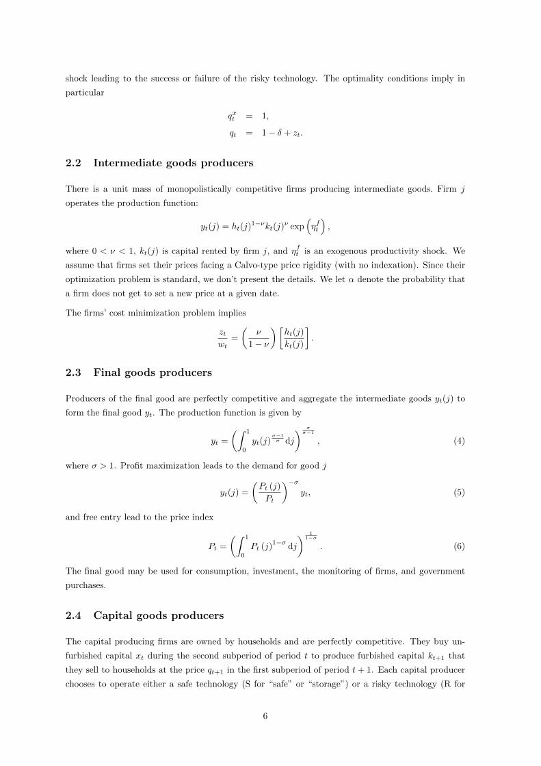
2.4 Capital goods producers
The capital producing firms are owned by households and are perfectly competitive. They buy un-
furbished capital xt during the second subperiod of period t to produce furbished capital kt+1 that
they sell to households at the price qt+1 in the first subperiod of period t+ 1. Each capital producer
chooses to operate either a safe technology (S for “safe” or “storage”) or a risky technology (R for
6
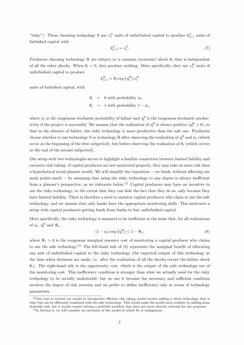
“risky”). Those choosing technology S use xSt units of unfurbished capital to produce kSt+1 units of
furbished capital with
kSt+1 = xSt . (7)
Producers choosing technology R are subject to a common (systemic) shock θt that is independent
of all the other shocks. When θt = 0, they produce nothing. More specifically, they use xRt units of
unfurbished capital to produce
kRt+1 = θt exp(ηRt)xRt
units of furbished capital, with
θt = 0 with probability φt,
θt = 1 with probability 1− φt,
where φt is the exogenous stochastic probability of failure and ηRt is the exogenous stochastic produc-
tivity if the project is successful. We assume that the realization of ηRt is always positive (ηRt > 0), so
that in the absence of failure, the risky technology is more productive than the safe one. Producers
choose whether to use technology S or technology R after observing the realization of ηRt and φt (which
occur at the beginning of the first subperiod), but before observing the realization of θt (which occurs
at the end of the second subperiod).
Our setup with two technologies serves to highlight a familiar connection between limited liability and
excessive risk taking: if capital producers are not monitored properly, they may take on more risk than
a hypothetical social planner would. We will simplify the exposition − we think, without affecting our
main points much − by assuming that using the risky technology to any degree is always inefficient
from a planner’s perspective, as we elaborate below.12 Capital producers may have an incentive to
use the risky technology, to the extent that they can hide the fact that they do so, only because they
have limited liability. There is therefore a need to monitor capital producers who claim to use the safe
technology, and we assume that only banks have the appropriate monitoring skills. This motivates a
setup with capital producers getting funds from banks to buy unfurbished capital.
More specifically, the risky technology is assumed to be inefficient in the sense that, for all realizations
of φt, ηRt and Ψt,
(1− φt) exp(ηRt)≤ 1−Ψt, (8)
where Ψt > 0 is the exogenous marginal resource cost of monitoring a capital producer who claims
to use the safe technology.13 The left-hand side of (8) represents the marginal benefit of allocating
one unit of unfurbished capital to the risky technology (the expected output of this technology at
the time when decisions are made, i.e. after the realization of all the shocks except the failure shock
θt). The right-hand side is the opportunity cost, which is the output of the safe technology net of
the monitoring cost. This inefficiency condition is stronger than what we actually need for the risky
technology to be socially undesirable; but we use it because the necessary and sufficient condition
involves the degree of risk aversion and we prefer to define inefficiency only in terms of technology
parameters.
12One way to extend our model to incorporate efficient risk taking would involve adding a third technology that isrisky but can be efficiently combined with the safe technology. This would make the model more realistic by adding somedesirable risk, but it would require solving a portfolio problem that does not seem directly relevant for our purposes.
13In Section 6, we will consider an extension of the model in which Ψt is endogenous.
7

Our model simplifies (we think in a harmless way) the relationship between capital goods producers,
their owners, and the creditor banks. In reality non-bank firms prefer debt finance because they get
a tax deduction. They also need some equity, presumably because of the agency problem associated
with debt. Their owners absorb losses up to their equity stake. In our model, for simplicity, we
abstract from this agency problem and capital goods producers have no equity. So this translates into
a framework in which their funding is entirely with loans and they pay no tax; and any profits or
losses arising from stochastic disturbances in the absence of failure of the risky technology accrue to
households.14 Thus, a capital producer i choosing technology j ∈ {S,R} borrows
qxt xjt (i) = ljt (i) (9)
at a nominal interest rate Rjt .15 Since capital producers have limited liability, those using the risky
technology will default on their loans in the event of failure (when θt = 0).
A producer i using technology S chooses xSt (i) to maximize
βEt
{λt+1
λt
[qt+1k
St+1 (i)− 1 +RSt
Πt+1lSt (i)
]}subject to (7) and (9). The optimality condition implies
Et {λt+1qt+1} = Et
{λt+1
Πt+1
}(1 +RSt
)qxt . (10)
A producer i using technology R chooses xRt (i) to maximize
(1− φt)βEt{λt+1
λt
[qt+1 exp
(ηRt)xRt (i)− 1 +RRt
Πt+1lRt (i)
]∣∣∣∣ θt = 1
}subject to (9), where Et { .| θt = 1} denotes the expectation operator conditional on the information
available in the first subperiod of period t and on the success of the risky technology in the second
subperiod of period t. The optimality condition implies
Et {λt+1qt+1| θt = 1} exp(ηRt)
= Et
{λt+1
Πt+1
∣∣∣∣ θt = 1
}(1 +RRt
)qxt . (11)
Since our model allows for two distinct interest rates, banks need to monitor the capital producers
that borrow at the lower rate to ensure that they use the associated technology. Our model has no
equilibrium with RRt < RSt .16 Therefore, there is no need for banks to monitor capital producers
that claim to use the risky technology. Accordingly, we will associate a cost with monitoring capital
producers that claim to use the safe technology.
As usual, with constant returns to scale, the first-order conditions imply that firms make zero profits.
When both (10) and (11) hold, capital producers are indifferent between the two technologies and
1 +RRt1 +RSt
=Et {λt+1qt+1| θt = 1}
Et {λt+1qt+1}
Et
{λt+1
Πt+1
}Et
{λt+1
Πt+1
∣∣∣ θt = 1} exp
(ηRt)
. (12)
If the interest-rate ratio on the left-hand side is strictly higher than the critical value on the right-hand
side, then capital producers use only technology S.
14Our results however would be qualitatively unchanged if capital goods producers were allowed to borrow only afraction of the funds they need, or if they only needed funding to pay for the investment flow (and financed the restwith equity).
15There is no need to work with nominal loan contracts in our model. However, since we will assume that monetarypolicy sets a nominal interest rate, and for the sake of realism, we make loan contracts nominal.
16Indeed, if we had RRt < RS
t , then funding the safe projects would strictly dominate funding the risky projectsbecause it would pay more in every state (whatever the realization of θt) and incur no monitoring cost.
8
2.5 Banks
Banks are owned by households. They are perfectly competitive. They incur a cost ΨtlSt of monitoring
safe loans, where Ψt satisfies (8). They can fund their loans by raising equity (et) or issuing deposits
(dt). They make safe and risky loans (lSt and lRt ). Their balance-sheet identity is
lSt + lRt = et + dt, (13)
as et is defined net of monitoring costs.
Under our assumptions (inefficiency condition (8), risk aversion, and no correlation between θt and
other shocks), risky projects reduce welfare. So if the regulators could detect any risky project, they
would devise a sufficient penalty to prevent it. We need an information friction to rule out a trivial
and unrealistic solution in which the regulators directly forbid risk taking. Following Van den Heuvel
(2008), we assume that banks can hide some risky loans in their portfolio from regulators. More
specifically, we assume that regulators observe the total amount of loans made by each bank but
cannot detect its risky loans up to an exogenous fraction γt of its safe loans. The prudential authority
imposes risk-weighted capital requirements on risky loans above this fraction. We specify the capital
requirement as
et ≥ κt(lSt + lRt
)+ κmax
{0, lRt − γtlSt
}. (14)
The higher the capital requirement, the more banks internalize the social cost of risk, as they have
more “skin in the game.” The prudential authority will optimally choose a sufficiently high κ for
lRt ≤ γtlSt in equilibrium. Therefore, this is equivalent to rewriting the capital requirement as a
minimum ratio of equity to loans:
et ≥ κt(lSt + lRt
), (15)
and imposing the following constraint on banks:
lRt ≤ γtlSt . (16)
In the first subperiod of period t + 1, regulators close the banks that cannot meet their deposit
obligations: the banks with
1 +RStΠt+1
lSt + θt1 +RRtΠt+1
lRt −1 +RDtΠt+1
dt < 0,
or equivalently, using (13), those with
et < −(RSt −RDt1 +RDt
)lSt −
(θt
1 +RRt1 +RDt
− 1
)lRt .
When lRt = 0 or θt = 1, the right-hand side of this inequality is negative as long as lending rates are
above the deposit rate, which will be the case in equilibrium because loans either incur a monitoring
cost or entail a risk for banks. When lRt > 0 and θt = 0, the right-hand side of this inequality is
positive if and only if
lRt >
(RSt −RDt1 +RDt
)lSt .
We want our model to capture the fact that banks find equity finance more costly than debt finance
in reality. We attribute this to a tax distortion (tax deduction for debt finance), although this
9
interpretation is not essential for our analysis. We take this distortionary tax to be a feature of the
environment: the model does not explain why this tax is in place, and the policymakers in our model
(the monetary and prudential authorities) cannot set this tax optimally.17
The particular way we specify the tax distortion (and the timing of the tax deduction for monitoring
costs) ensures that unanticipated changes in the price level cannot cause insolvency.18 The banks
in our model may be insolvent only if they extend too many risky loans, and the risky projects fail.
Specifically, we assume that gross revenues from loans are taxed at the constant rate τ after deductions
for gross payments on deposits and monitoring costs. The amount of bank equity, net of monitoring
costs, is therefore et = qbtst − (1− τ)ΨtlSt .
The representative bank chooses et, dt, lRt and lSt to maximize
Et
{βλt+1 (1− τ)ωbt+1
λt
}− et − (1− τ) Ψtl
St ,
where
ωbt+1 = max
{0,
1 +RStΠt+1
lSt + θt1 +RRtΠt+1
lRt −1 +RDtΠt+1
dt
}, (17)
subject to (13), (15) and (16).
2.6 Government and market-clearing conditions
The government has exogenous purchases Gt and guarantees bank deposits. The lump-sum tax on
households balances the budget.19
The losses imposed by bank j on the deposit insurance fund amount to
ζt(j) = max
{0,
1 +RDt−1
Πtdt−1(j)−
1 +RSt−1
ΠtlSt−1(j)− θt−1
1 +RRt−1
ΠtlRt−1(j)
},
and the lump-sum tax paid by households is
τht = Gt +
∫ 1
0
{ζt(j)− τ [ωbt (j) + Ψtl
St (j)]
}dj.
We consider two policy instruments: the deposit rate RDt for monetary policy and the capital require-
ment κt for prudential policy. We will discuss our specifications of prudential policy in Sections 3 and
5. For each specification, our monetary policy will be the Ramsey-optimal policy.
Firms producing intermediate goods rent their capital from the representative household; in equilib-
rium, their choices must satisfy ∫ 1
0
kt(j )dj = k t.
Similarly obvious market-clearing conditions must be satisfied in the markets for labor, loans, and
unfurbished capital. The market-clearing condition for goods is
ct + it +Gt + ΨtlSt = yt.
17This feature of the tax code seems to be one of the primary reasons for banks to lobby against higher capitalrequirements, at least in the US and the euro area. It is commonly invoked in models with both debt and equityfinance [e.g. Jermann and Quadrini (2009, 2012)], to break the Modigliani-Miller theorem about irrelevance of financialstructure. We motivate our modeling choice in the conclusion.
18In our setting with one-period competitive banks incurring real monitoring costs and extending nominal loans, achange in the price level could lead to insolvency. We don’t think this is an interesting feature of the model and havespecified our “tax code” to rule it out.
19It is harmless to abstract from deposit insurance fees paid by banks and include these in the lump-sum tax paid byhouseholds who own the banks.
10
3 Prudential Policy
This section derives conditions for prudential policy to rule out equilibria with risk taking and ensure
the existence of equilibria without risk taking. We first show that our model can only have equilibria
at the two corners with lRt = 0 and lRt = γtlSt , and that the capital constraint is binding in any
equilibrium. Next, we consider a benchmark prudential policy that internalizes the externality (arising
from limited liability) by making banks the residual claimants to any losses they may incur. We then
characterize the least stringent prudential policy that rules out risk taking, and show that it is locally
Ramsey-optimal.
3.1 Ruling out candidate equilibria
We focus on symmetric equilibria in which all banks have the same loan portfolio. We will also assume
throughout that the following condition holds:
Et {λt+1qt+1| θt = 1}Et {λt+1qt+1}
≤ 1. (18)
This condition seems plausible because failure of risky projects at date t leads to destruction of the
capital stock at date t+ 1, and this by itself should increase both the price of capital (qt+1) and the
marginal utility of consumption (λt+1). However, this condition amounts to an implicit restriction
on the set of policies that we consider, as it presumes that policies will not overturn the qualitative
effects of the failure of risky projects.
We first show that the banks’ optimization problem rules out the existence of equilibria with 0 < lRt <
γtlSt . The basic insight follows Van den Heuvel (2008), but since we have added aggregate risk and
made other changes to his model, we prove the following proposition in the Appendix.
Proposition 1: There are no equilibria with 0 < lRt < γtlSt . When 0 < lRt < γtl
St , (a) if banks go
bankrupt (ωbt+1 = 0) when risky projects fail ( θt = 0), then banks can increase their market value by
tilting the loan portfolio towards more risky loans; (b) if banks do not go bankrupt (ωbt+1 > 0) when
risky projects fail ( θt = 0), then they can increase their market value by tilting the loan portfolio
towards more safe loans.
The intuition follows. If, given the loan portfolio, bank equity is sufficiently small to be wiped out
when risky projects fail, then banks do not internalize the cost of additional risk taking. Additional
losses from increasing lRt , if risky projects fail, are truncated by deposit insurance and limited liability.
Consequently, the only candidate for an equilibrium with the possibility of bank failure involves the
corner solution lRt = γtlSt .
Alternatively, if bank equity is sufficiently large for banks to remain solvent even when risky projects
fail, then banks internalize the cost of additional risk taking. In that case, since we assume that the
risky technology is inefficient, banks can increase their market value by reducing lRt . Accordingly, the
only candidate for an equilibrium without the possibility of bank failure involves the corner solution
lRt = 0. In particular, if bank equity is large enough to make banks residual claimants on their risky
loans when lRt = γtlSt , then there does not exist an equilibrium with lRt = γtl
St .
11

Next, we show that there are no equilibria in which the capital constraint is lax:
Proposition 2: In equilibrium, the capital constraint is binding:
et = κt(lSt + lRt
). (19)
This Proposition follows almost directly from our assumption about the tax advantage of debt finance
over equity finance, but we provide a proof in the Appendix.
3.2 A benchmark policy
Proposition 1 leads to a sufficient condition for prudential policy to rule out equilibria with lRt > 0 and
ensure the existence of an equilibrium with lRt = 0: the capital requirement can be sufficiently high to
make any bank the residual claimant to the potential losses arising from funding risky projects. This
benchmark policy is characterized by the following proposition:
Proposition 3: (a) A sufficient condition for existence and uniqueness of an equilibrium and for
lRt = 0 in this equilibrium is that
κt > κ(RDt , R
St
)≡ 1− 1
1 + γt
1 +RSt1 +RDt
; (20)
(b) in this equilibrium,
κ(RDt , R
St
)= κt ≡
(1− τ) (γt −Ψt)
τ + (1− τ) (1 + γt); (21)
(c) κt is increasing in γt, and decreasing in Ψt.
We prove this proposition in the Appendix, by considering a given bank j that takes the maximum
amount of risk (lRt (j) = γtlSt (j)). We show that this bank will remain solvent when risky projects
fail (θt = 0) if and only if (20) holds. We then use the banks’ optimality conditions at the equilibrium
with lRt = 0 to express κ(RDt , R
St
)in terms of parameters and exogenous shocks and obtain (21).
We assume γt > Ψt, which implies κt > 0, so that condition (20) may or may not be met depending
on the value of κt. This restriction states that the temptation to take risk would be present if banks
were not subject to any (positive) capital requirements. The threshold κt is increasing in γt: the
higher the fraction of risky loans that a deviating bank can hide, the riskier this bank, and the higher
the capital requirement needed to make it remain solvent in case of failure. And κt is decreasing in
Ψt: the higher the cost of monitoring safe loans, the higher the spread between the interest rate on
safe loans and that on deposits; thus, the larger the cash flow from safe loans that is available to
redeem the deposits, and the lower the capital requirement needed to make a deviating bank remain
solvent in case of failure.
Although this benchmark policy suffices to ensure the existence of an equilibrium without risk taking,
we show next that it is more stringent than necessary and that the least stringent policy ensuring the
existence of an equilibrium without risk taking is locally Ramsey-optimal in our model.
12

3.3 The locally optimal policy
We now derive a necessary and sufficient condition for prudential policy to ensure the existence of
an equilibrium with lRt = 0, and then show that the least stringent policy satisfying this condition is
locally Ramsey-optimal.
Consider a bank j that deviates from a candidate equilibrium with lRt = 0 to take the maximum
amount of risk (lRt (j) = γtlSt (j)). There exists an equilibrium with lRt = 0 if and only if this deviating
bank has a negative expected excess return. In the Appendix, we derive the threshold value of κt that
makes its expected excess return negative, and we prove the following proposition:
Proposition 4: (a) A necessary and sufficient condition for existence of an equilibrium with lRt = 0
is κt ≥ κ∗t , where
κ∗t ≡ (1− τ)(1− φt) γt
[exp
(ηRt)− 1]
+ Ψt
[(1− φt) γt exp
(ηRt)− φt
]φt (1 + γt)− γtτ (1− φt)
[exp
(ηRt)− 1] ; (22)
(b) κ∗t < κt; (c) κ∗t is increasing in the probability of success of the risky technology 1 − φt, the
productivity of the risky technology conditionally on its success ηRt , and the maximum ratio of risky to
safe loans γt.
The derivations in the Appendix consider a bank j that contemplates a deviation from a candidate
equilibrium with lRt = 0. The same intuition we gave for Proposition 1 (roughly) applies: if there are
profitable deviations, the most profitable one is at the corner with maximum risk (lRt (j) = γtlSt (j)).
To derive the value of κ∗t , we make bank j indifferent between staying at the safe corner and moving
to the risky corner. The bank turns indifferent with less equity at stake than what would make it
residual claimant (i.e., we have κ∗t < κt) because the bank has incurred monitoring costs and has a
vested interest in remaining solvent to recoup these costs. In a way, monitoring costs in our model
work like giving the banks some charter value that they would like to preserve by avoiding bankruptcy.
The preceding intuition also helps us understand the nature of the state dependence, in our model,
of the constraint κt ≥ κ∗t . Macro-prudential policy must be tight enough to prevent risk taking in
equilibrium. The threshold κ∗t depends negatively on the probability of failure of the risky technology
φt because failure risk, by itself, makes risk-taking less attractive. Similarly, κ∗t rises with the produc-
tivity of the risky technology conditionally on its success ηRt and with the maximum ratio of risky to
safe loans γt.20
Perhaps a more surprising feature of (22) is that κ∗t does not depend on the monetary policy instrument
RDt . This is because, in our model, the deposit rate RDt does not affect banks’ incentives for risk taking.
In particular, it does not affect the spread between the interest rate on risky loans RRt and the interest
rate on safe loans RSt . In a way, this is not a surprising feature for a model with perfect competition
and constant returns. Our banks never run out of safe projects to fund and always end up making zero
profits. This is the opposite extreme from arguments that (explicitly or implicitly) postulate a fixed
number of potential projects and thereby link more lending with more risk taking (as banks run out
20Our model could be extended to allow the prudential authority to choose γt by incurring some supervision cost, asin Van den Heuvel (2008). This would not change the optimal solution for κt as a function of γt in (22), but wouldmake γt endogenous. In this case, the prudential authority would optimally respond to shocks that increase risk-takingincentives by devoting more resources to supervision (i.e. lowering γt) and raising the capital requirement κt by less.
13
of safe lending opportunities). We will revisit this contrast between extreme modelling assumptions
in Section 6.
We now turn to normative implications. We define locally Ramsey-optimal policies as follows: a
policy (RDτ , κτ )τ≥0 is locally Ramsey-optimal if there exists a neighborhood of (RDτ , κτ )τ≥0 such that
no other policy in this neighborhood gives a higher value for the representative household’s expected
utility than (RDτ , κτ )τ≥0 does. Let(RD∗τ
)τ≥0
denote the monetary policy that is (globally) Ramsey-
optimal when the prudential policy is (κ∗τ )τ≥0. The following proposition states that, under a certain
condition, setting jointly(RDτ)τ≥0
to(RD∗τ
)τ≥0
and (κτ )τ≥0 to (κ∗τ )τ≥0 is locally Ramsey-optimal:
Proposition 5: If the right derivative of welfare with respect to κt at(RDτ , κτ
)τ≥0
=(RD∗τ , κ∗τ
)τ≥0
is
strictly negative for all t ≥ 0, then the policy(RDτ , κτ
)τ≥0
=(RD∗τ , κ∗τ
)τ≥0
is locally Ramsey-optimal.
We prove this proposition in the Appendix. The basic idea is the following. First, whatever RDt in
the neighborhood of RD∗t , setting κt just below κ∗t is not optimal, because it triggers a discontinuous
increase in the amount of risk taken by banks. Under our assumptions (inefficiency condition (8), risk
aversion, and no correlation between θt and other shocks), this discontinuous increase in the amount
of risk has a discontinuous negative effect on welfare. Any other effect on welfare is continuous and,
therefore, dominated by this discontinuous negative effect provided that(RDt , κt
)is close enough to(
RD∗t , κ∗t). Second, if the right derivative of welfare with respect to κt at
(RD∗t , κ∗t
)is strictly negative,
then setting κt just above κ∗t is not optimal either, because it has a negative first-order effect on welfare
that cannot be offset by any change in RDt around its optimal value RD∗t (as this change would have
a zero first-order effect on welfare).
The right derivative of welfare with respect to κt at(RD∗t , κ∗t
)can be expected to be strictly negative
because increasing κt from κ∗t decreases the capital stock, which is already inefficiently low due to the
monopoly and tax distortions, without reducing the amount of risk, which is already zero. We check
numerically, for the calibration considered in the next section, that this derivative is indeed strictly
negative. This derivative is equal to the Lagrange multiplier associated to the constraint κt = κ∗t
in the optimization problem that determines RD∗τ . We first use the program Get Ramsey developed
by Levin and Lopez-Salido (2004) and used in Levin, Onatski, Williams and Williams (2005) to get
analytically the non-linear first-order conditions of this optimization problem. We then use Dynare
to solve numerically, at the first order, the resulting system of constraints and first-order conditions,
and thus get the first-order approximation of this Lagrange multiplier (among other variables). We
check that this Lagrange multiplier is strictly negative at the steady state, which implies that it is
strictly negative for small enough shocks. We also check that it is strictly negative at the first order
in the presence of shocks of a standard size.
We suspect (but cannot verify) that the policy (RD∗τ , κ∗τ )τ≥0 that we have identified is the globally
Ramsey-optimal policy when failure of the risky technology is sufficiently costly, given the distortions
present in our model. As noted above, values of κt higher than κ∗t bring no additional benefit in
terms of reducing risk, and are costly because they reduce the capital stock further. Values of κt lower
than κ∗t have the benefit of increasing the capital stock as long as risky projects succeed, and the
drawback of recurrent falls in the capital stock. Computing equilibria of our model with κt ≤ κ∗t (e.g.
κt = 0) under Ramsey-optimal monetary policy cannot be achieved using log–linearization techniques
because our model involves expectations conditional on the realization of a binary shock. This calls
14

for global approximation techniques which, under Ramsey-optimal policy, would suffer the curse of
dimensionality given the number of state variables this equilibrium generates.21
3.4 Ruling out equilibria with lRt = γtlSt
We next formulate a prudential feedback rule that precludes equilibria with lRt = γtlSt , and coincides
with κt = κ∗t in equilibrium. That is, under this rule, there is a unique equilibrium and, in this
equilibrium, lRt = 0 and κt takes the minimum value that is consistent with lRt = 0.
We will assume throughout that the following condition holds:
Et
{λt+1
Πt+1
∣∣∣ θt = 1}
Et
{λt+1
Πt+1
} ≤ 1. (23)
This condition seems plausible but, as we noted in our discussion of (18), it amounts to an implicit
restriction on the set of policies that we consider.22
We prove the following proposition in the Appendix:
Proposition 6: Under the prudential-policy rule
κt =1− φtφt
γt1 + γt
RRt −RSt1 +RDt
+1
φt
γt1 + γt
Ψt −RSt −RDt1 +RDt
, (24)
there exists a unique equilibrium and, in this equilibrium, lRt = 0 and κt = κ∗t .
Although the formal proof in the Appendix takes a different approach, a heuristic rendition is to
start with the equilibrium at the safe corner and define RRt as the highest rate that a deviating bank
could charge on a loan to a risky firm. In this case, (24) just states κ∗t as a function of interest-rate
spreads. It gives the critical value of κt for making the bank indifferent between staying at the safe
corner (where all the other banks are) and jumping to the risky corner. The critical value is fairly
intuitive. The first two terms represent the temptation to deviate from the safe corner to the risky
corner: a deviating bank will pocket RRt −RSt if risky projects succeed (with probability 1− φt) and
save monitoring costs. The third term represents the opportunity cost RSt − RDt of this deviation
when risky projects fail (with probability φt).
So, this feedback rule suffices for keeping banks at the safe corner. In the Appendix we show that it
also suffices to rule out an equilibrium at the risky corner, because the safe corner becomes even more
attractive to an individual bank if there is a mass of banks at the risky corner (in which case the risk
is priced).
4 Calibration
The parameters pertaining to households and firms are standard. For the parameters pertaining to
the banking sector, we build heavily on Van den Heuvel (2008). The period of time is a quarter.
21The set of state variables includes the capital stock, price dispersion, the shocks and the Lagrange multipliersassociated to the forward-looking constraints of the Ramsey-optimization problem − a total of 13 state variables.
22The condition seems plausible when we consider the pricing of a bond with default risk − a bond that pays $1 whenrisky projects succeed and pays nothing when they fail. The inequality (23) says this risky bond has a higher expectedreal return, compared to a nominal bond with no default risk, in the equilibria we consider.
15
The discount rate is such that the household discounts the future at the deposit rate, 2.76% per year
(see Van den Heuvel, 2008). The labor supply elasticity is set to 1. The value of the elasticity of
substitution between intermediate goods σ is related to the degree of monopoly power firms have.
Estimates of markups fall in the 10–20 percent range, implying that the elasticity of substitution lies
in the 6–11 range. We follow Golosov and Lucas (2007) and set the elasticity of substitution to 7,
implying a firms’ markup of about 16 percent.
The capital elasticity in the intermediate-good technology is set such that the labor share is 0.66,
implying a value for ν of 0.3. The depreciation rate, δ, is set to 0.025, which corresponds to a 10%
annual depreciation rate. Firms are assumed to reset their prices every 3 quarters on average, implying
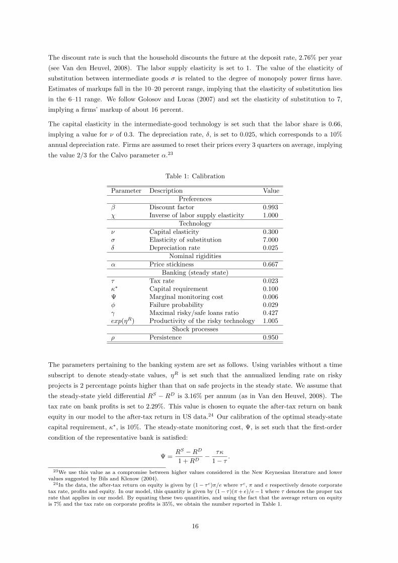
the value 2/3 for the Calvo parameter α.23
Table 1: Calibration
Parameter Description ValuePreferences
β Discount factor 0.993χ Inverse of labor supply elasticity 1.000
Technologyν Capital elasticity 0.300σ Elasticity of substitution 7.000δ Depreciation rate 0.025
Nominal rigiditiesα Price stickiness 0.667
Banking (steady state)τ Tax rate 0.023κ∗ Capital requirement 0.100Ψ Marginal monitoring cost 0.006φ Failure probability 0.029γ Maximal risky/safe loans ratio 0.427exp(ηR) Productivity of the risky technology 1.005
Shock processesρ Persistence 0.950
The parameters pertaining to the banking system are set as follows. Using variables without a time
subscript to denote steady-state values, ηR is set such that the annualized lending rate on risky
projects is 2 percentage points higher than that on safe projects in the steady state. We assume that
the steady-state yield differential RS − RD is 3.16% per annum (as in Van den Heuvel, 2008). The
tax rate on bank profits is set to 2.29%. This value is chosen to equate the after-tax return on bank
equity in our model to the after-tax return in US data.24 Our calibration of the optimal steady-state
capital requirement, κ∗, is 10%. The steady-state monitoring cost, Ψ, is set such that the first-order
condition of the representative bank is satisfied:
Ψ =RS −RD
1 +RD− τκ
1− τ.
23We use this value as a compromise between higher values considered in the New Keynesian literature and lowervalues suggested by Bils and Klenow (2004).
24In the data, the after-tax return on equity is given by (1− τc)π/e where τc, π and e respectively denote corporatetax rate, profits and equity. In our model, this quantity is given by (1− τ)(π+ e)/e− 1 where τ denotes the proper taxrate that applies in our model. By equating these two quantities, and using the fact that the average return on equityis 7% and the tax rate on corporate profits is 35%, we obtain the number reported in Table 1.
16
This yields the value Ψ = 0.006. The steady-state failure probability of risky projects φ and the
steady-state maximal risky/safe loans ratio γ are set jointly such that the model matches the average
failure rate in the US economy (0.86% per quarter) and the optimal steady-state capital requirement
is 10%:
γφ
1 + γ= 0.86 and (1− τ)
(1− φ) γ[exp
(ηR)− 1]
+ Ψ[(1− φ) γ exp
(ηR)− φ
]φ (1 + γ)− γτ (1− φ) [exp (ηR)− 1]
= 0.10.
This system leads to a quadratic equation in γ, which has a unique positive solution, equal to 0.427,
from which we get φ = 0.029. The persistence of all the shocks is set to ρ = 0.95.25 For the impulse-
response functions presented in the next section, we set the innovations to the technology shock ηft
and the fiscal shock Gt equal to 1%, and the innovation to Ψt to 10%. We set the innovation to ηRt
such that the annualized risk premium increases from 2% to 3%. And we set the innovation to φt
such that the probability of failure increases by 1/3 of a percentage point.
5 Numerical Results
We consider two alternative prudential policies. Our benchmark prudential policy sets κt equal to
its locally Ramsey-optimal value κ∗t , which is 0.10 at the steady state. The other policy keeps κt
constant at 0.12. This value is high enough, given the size of our shocks, to keep the economy in the
safe equilibrium.
For each of these prudential policies, we solve for the Ramsey monetary policy using Dynare and
the program Get Ramsey developed by Levin and Lopez-Salido (2004). In both cases, the optimal
steady-state inflation rate is zero, given the presence of Calvo-type price rigidity and the absence of
monetary distortions in our model.
Figure 1 displays the optimal responses to a favorable productivity shock (positive innovation to
ηft ). The responses, with the exception of those of the interest rates, are expressed as percentage
deviations from each steady state. The response of the interest rates is measured in terms of the
level of the interest rate as a percentage per annum (rather than a deviation from the steady state).
The horizontal dashed line corresponds to the steady-state level of the interest rate, so values below
this line represent accommodative monetary policy following the shock, and values above represent
restrictive monetary policy.
Since a productivity shock does not create a temptation to take more risk in our model, it does
not affect the optimal capital requirement κ∗t . So the optimal responses of the policy rate, output
and inflation are the same, regardless of the prudential policy in place (κt = κ∗t or κt = 0.12).
These optimal responses to a productivity shock are qualitatively similar to optimal responses in the
benchmark New-Keynesian (NK) model with capital. Optimal policy essentially keeps inflation at
zero. This requires an increase in the deposit rate for a while, because the natural real interest rate
rises in the model with capital.26 Optimal responses to an increase in government purchases (not
reported here) are also similar to those from the NK model, and independent of prudential policy.
25Note that in order to study the response of the economy to shocks to the failure rate, we assume that φt =(1 + exp(−(ut − v)))−1 where ut is assumed to follow a zero-mean AR(1) process and v = 3.393.
26Both the favorable productivity shock and the resulting increase in employment increase the marginal product ofcapital.
17

Figure 1: Response to a Favorable Productivity Shock (ηft )
0 5 10 15 20
0.7
0.8
0.9
1
1.1
1.2
1.3
Output
Periods
Per
c. d
ev.
0 5 10 15 20−2
−1
0
1
2Inflation Rate
Periods
Ann
ualiz
ed R
ate
(%)
0 5 10 15 20
2.7
2.75
2.8
2.85
2.9
2.95Deposit Rate
Periods
Ann
ualiz
ed R
ate
(%)
0 5 10 15 209
10
11
12
13Capital Requirement
Periods
Per
cent
ages
κt = κ∗t κt = 0.12 Dashed line: Steady-State Level
Figure 2: Response to an Increase in the Productivity of the Risky Technology (ηRt )
0 5 10 15 20
−0.25
−0.2
−0.15
−0.1
−0.05
0
0.05
Output
Periods
Per
c. d
ev.
0 5 10 15 20−2
−1
0
1
2Inflation Rate
Periods
Ann
ualiz
ed R
ate
(%)
0 5 10 15 202.55
2.6
2.65
2.7
2.75
2.8Deposit Rate
Periods
Ann
ualiz
ed R
ate
(%)
0 5 10 15 209
10
11
12
13Capital Requirement
Periods
Per
cent
ages
κt = κ∗t κt = 0.12 Dashed line: Steady-State Level
18
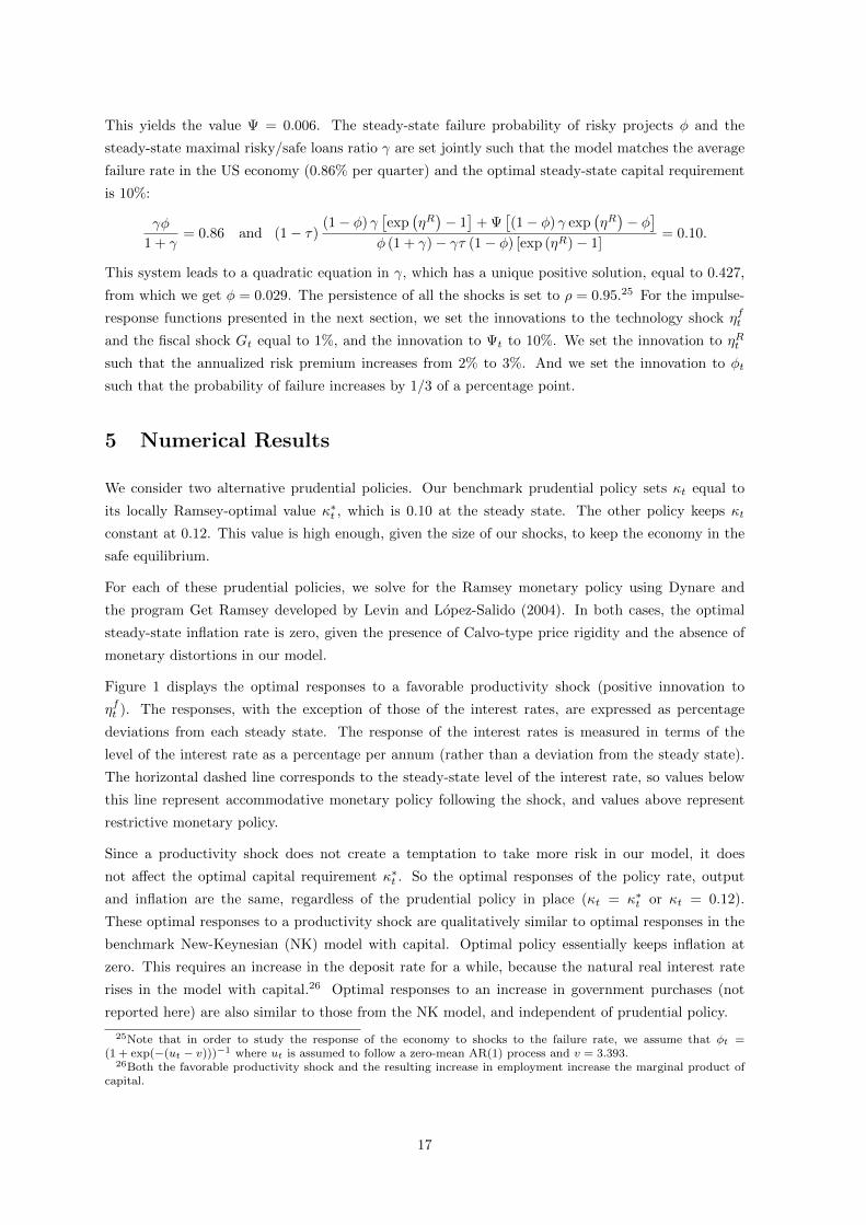
A positive shock to ηRt is a pure temptation for banks and firms to deviate from the safe equilibrium; it
increases the return on risky projects in case they succeed. Figure 2 shows that this shock increases the
capital requirement under the optimal prudential policy (κt = κ∗t ). By itself, the tightening of capital
requirements increases the cost of banking in our model. The optimal monetary-policy response is to
cut the deposit rate in order to curb the increase in bank lending rates. The overall effects on output
are small, and inflation is essentially zero under optimal policy.
We find this thought experiment quite useful in the context of policy-oriented discussions [e.g., Canuto
(2011), Cecchetti and Kohler (2012), Macklem (2011), Wolf (2012), Yellen (2010)] of how monetary
and prudential policies may be substitutes for each other or move to offset each other’s effects. In our
case, one policy is contractionary and the other expansionary in order to manage risk-taking incentives
with the smallest possible adverse effects on investment.
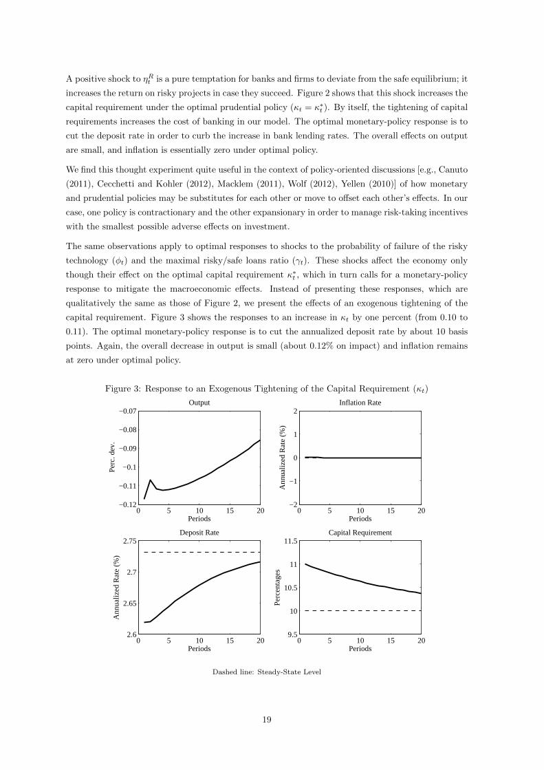
The same observations apply to optimal responses to shocks to the probability of failure of the risky
technology (φt) and the maximal risky/safe loans ratio (γt). These shocks affect the economy only
though their effect on the optimal capital requirement κ∗t , which in turn calls for a monetary-policy
response to mitigate the macroeconomic effects. Instead of presenting these responses, which are
qualitatively the same as those of Figure 2, we present the effects of an exogenous tightening of the
capital requirement. Figure 3 shows the responses to an increase in κt by one percent (from 0.10 to
0.11). The optimal monetary-policy response is to cut the annualized deposit rate by about 10 basis
points. Again, the overall decrease in output is small (about 0.12% on impact) and inflation remains
at zero under optimal policy.
Figure 3: Response to an Exogenous Tightening of the Capital Requirement (κt)
0 5 10 15 20−0.12
−0.11
−0.1
−0.09
−0.08
−0.07Output
Periods
Per
c. d
ev.
0 5 10 15 20−2
−1
0
1
2Inflation Rate
Periods
Ann
ualiz
ed R
ate
(%)
0 5 10 15 202.6
2.65
2.7
2.75Deposit Rate
Periods
Ann
ualiz
ed R
ate
(%)
0 5 10 15 209.5
10
10.5
11
11.5Capital Requirement
Periods
Per
cent
ages
Dashed line: Steady-State Level
19

Figure 4: Response to an Increase in the Cost of Making Safe Loans (Ψt)
0 5 10 15 20−0.2
−0.18
−0.16
−0.14
−0.12
−0.1
−0.08Output
Periods
Per
c. d
ev.
0 5 10 15 20−2
−1
0
1
2Inflation Rate
Periods
Ann
ualiz
ed R
ate
(%)
0 5 10 15 202.45
2.5
2.55
2.6
2.65
2.7
2.75Deposit Rate
Periods
Ann
ualiz
ed R
ate
(%)
0 5 10 15 209
10
11
12
13Capital Requirement
Periods
Per
cent
ages
κt = κ∗t κt = 0.12 Dashed line: Steady-State Level
Figure 4 shows responses to a change in the marginal cost of making safe loans Ψt. In contrast to
the other shocks, this shock has direct macroeconomic effects in addition to its effects on the risk-
taking incentives of banks. Under a prudential policy keeping κt constant, this shock reduces output
in our model, and monetary policy cuts the deposit rate to mitigate this effect. Under the optimal
prudential policy (κt = κ∗t ), output falls more because, as we explained earlier, the increase in κt
(needed to prevent risk taking) increases bank lending rates. Monetary policy reacts to the tighter
capital requirements by cutting the deposit rate further.
How costly are policies that keep capital requirements constant (at a value high enough to ensure no
risk is taken), relatively to the optimal policy? Since our analysis is mainly qualitative, the answer of
our calibrated model to this question can, of course, be only suggestive, but we think it is nonetheless
informative. To address this question, we compute the welfare cost from unexpectedly switching at
date 0 from the optimal prudential policy (κt = κ∗t ) to a prudential policy setting κt to a constant
value κ equal to either 0.12 or 0.14, assuming that monetary policy is conducted optimally at all
dates. We measure this welfare cost by the value of foregone consumption, expressed as the fraction
of consumption each period under optimal policy, that would lead to the same welfare loss as the
change in policy does − i.e. by the parameter λ implicitly defined by
E∞∑t=0
βtU((1− λ)c∗t , h∗t ) = E
∞∑t=0
βtU(ct, ht)
where c∗t and h∗t denote consumptions and hours of work at date t under optimal policy, while ct and
ht denote consumptions and hours of work at date t in the case where the unexpected policy switch
occurs at date 0 (κτ = κ∗τ for τ < 0 and κτ = κ for τ ≥ 0). Following Benigno and Woodford (2006,
20

2012), the welfare computation is performed using a second order perturbation method.
As we are moving from one steady state to another (reached asymptotically), we have to take into
account the cost of transition. The first column of Table 2 computes the welfare cost of transiting
from one steady state to the other (including the cost of fluctuations due to non-linearities along the
way). It is positive because moving from one steady state to the other reduces the capital stock, which
is already inefficiently low due to the monopoly and tax distortions. The second column computes
the welfare cost due to the difference in fluctuations around each steady state, ignoring the cost of
transiting from one steady state to the other. This cost is negative (i.e., corresponds to a welfare gain)
because fluctuations are smaller under constant capital requirements, as purely financial shocks (i.e.,
γt, ηRt , φt) are not transmitted to the economy. The last column reports the welfare loss associated to
both phenomena at the same time. It is positive because the transition cost dominates the fluctuations
gain.
Table 2: Welfare costs (percentage points)
Transition Fluctuations Total
κ=0.12 2.2750 -0.9918 1.2606κ=0.14 3.6704 -0.9465 2.6892
To summarize our main point, our model highlights a distinction across policy instruments that we
think deserves more emphasis than it gets in the existing literature: changes in the capital requirement
can directly manage risk-taking incentives, while changes in the policy interest rate cannot. When the
capital requirement rises to curb risk taking, a contraction ensues, and the policy interest rate is cut.
With this chain of causality, optimal prudential policy is pro-cyclical, and optimal monetary policy is
counter-cyclical.
Nonetheless, our model also provides a framework for thinking about some scenarios (or extensions)
that can make optimal prudential policy counter-cyclical, as we discuss below.
6 Extensions and Policy Concerns
Our benchmark model, while stylized, provide several useful insights. For example, as Angeloni and
Faia (2011) elaborate, the leading argument for Basel III-type counter-cyclical capital requirements
is the observation that default risk rises during recessions; and risk-weighted (Basel II-type) capital
requirements automatically tighten policy in recessions, unless the regulatory rate is lowered.27 Our
model suggests a reason for the latter to happen, that is, for cutting capital requirements when
default risk is high: When the banks have enough skin in the game, the additional risk makes banks
less inclined to fund risky projects, allowing prudential policy to set lower requirements without
undermining the stability of the banking system.
In this subsection, we illustrate how (admittedly ad hoc) extensions can provide additional insights.
We consider two extensions: externalities in bank lending, and correlation across shocks affecting the
27See Covas and Fujita (2010) for a quantitative assessment of the procyclical effects of bank capital requirementsunder Basel II.
21
incentives to take risks and shocks to the business cycle. We show that each of these two extensions
can make both policy instruments countercyclical under optimal policy. We also show that, although
the first extension gives rise to a risk-taking channel of monetary policy, it does not qualitatively affect
the optimal policy responses to shocks that directly affect risk-taking incentives.
6.1 An externality
Our model assumes perfect competition and constant returns in the banking sector. As we noted
earlier these assumptions imply that shocks that directly affect the optimal policy interest rate (like
standard productivity or fiscal shocks) do not affect the optimal bank-capital requirement. We now
consider a simple (ad-hoc) extension that links the cost of banking to the aggregate volume of safe
loans and thus allows such shocks to affect both policy margins. Hachem (2010) develops a model with
an externality in banking costs. In her model, banks ignore the effect of their own lending decision on
the pool of borrowers, with heterogeneous levels of risk, that is available to other banks.28 Here, we
only consider a simple example of such an externality − in order to preserve our earlier derivations
that treated Ψt as exogenous to the banks’ decisions − but we think this example highlights the main
features of policy interactions that arise when an economic boom increases risk-taking incentives.
Specifically, we assume
log(Ψt) = log(Ψ) + %[log(lSt )− log(lS)
](25)
where the term log(lSt ) − log(lS) is the log-deviation of the aggregate volume of safe loans from its
steady-state value, and % = 0 corresponds to our benchmark model. We show the impulse responses for
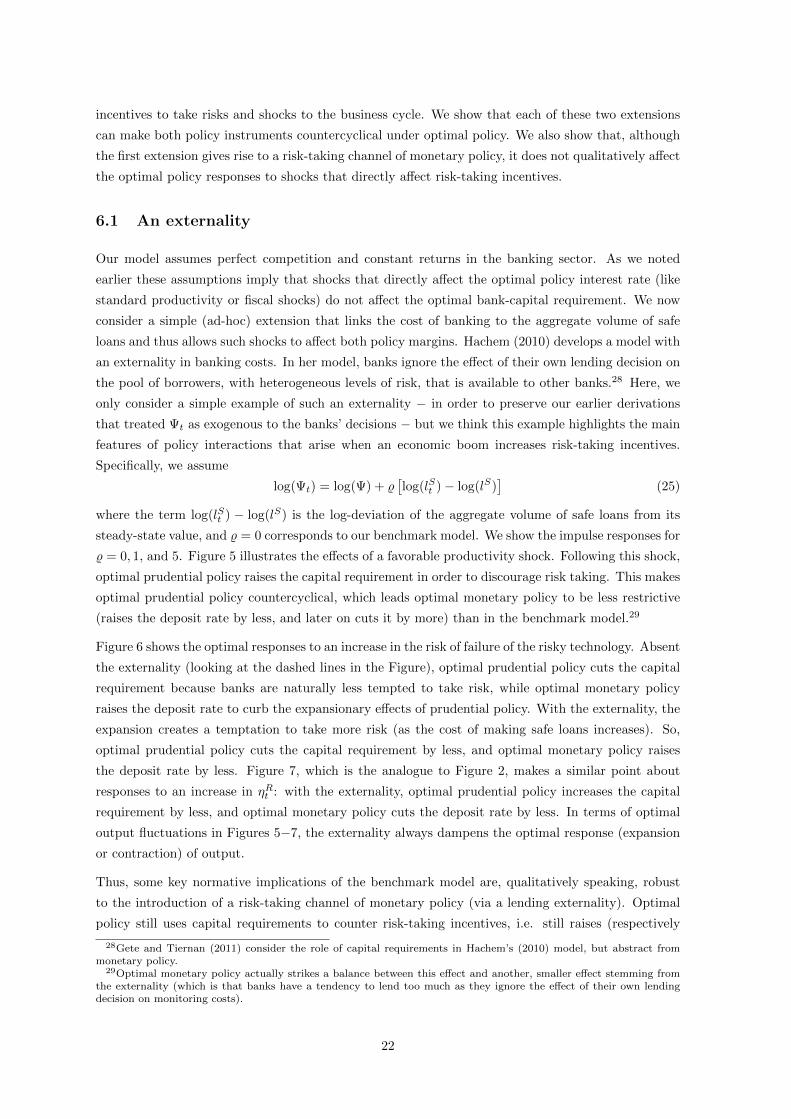
% = 0, 1, and 5. Figure 5 illustrates the effects of a favorable productivity shock. Following this shock,
optimal prudential policy raises the capital requirement in order to discourage risk taking. This makes
optimal prudential policy countercyclical, which leads optimal monetary policy to be less restrictive
(raises the deposit rate by less, and later on cuts it by more) than in the benchmark model.29
Figure 6 shows the optimal responses to an increase in the risk of failure of the risky technology. Absent
the externality (looking at the dashed lines in the Figure), optimal prudential policy cuts the capital
requirement because banks are naturally less tempted to take risk, while optimal monetary policy
raises the deposit rate to curb the expansionary effects of prudential policy. With the externality, the
expansion creates a temptation to take more risk (as the cost of making safe loans increases). So,
optimal prudential policy cuts the capital requirement by less, and optimal monetary policy raises
the deposit rate by less. Figure 7, which is the analogue to Figure 2, makes a similar point about
responses to an increase in ηRt : with the externality, optimal prudential policy increases the capital
requirement by less, and optimal monetary policy cuts the deposit rate by less. In terms of optimal
output fluctuations in Figures 5−7, the externality always dampens the optimal response (expansion
or contraction) of output.
Thus, some key normative implications of the benchmark model are, qualitatively speaking, robust
to the introduction of a risk-taking channel of monetary policy (via a lending externality). Optimal
policy still uses capital requirements to counter risk-taking incentives, i.e. still raises (respectively
28Gete and Tiernan (2011) consider the role of capital requirements in Hachem’s (2010) model, but abstract frommonetary policy.
29Optimal monetary policy actually strikes a balance between this effect and another, smaller effect stemming fromthe externality (which is that banks have a tendency to lend too much as they ignore the effect of their own lendingdecision on monitoring costs).
22

Figure 5: Response to a Favorable Productivity Shock (ηft )
0 5 10 15 20
0.4
0.6
0.8
1
1.2
Output
Periods
Per
c. d
ev.
0 5 10 15 20−2
−1
0
1
2Inflation Rate
Periods
Ann
ualiz
ed R
ate
(%)
0 5 10 15 20
2.7
2.75
2.8
2.85
2.9
2.95Deposit Rate
Periods
Ann
ualiz
ed R
ate
(%)
0 5 10 15 209.9
9.95
10
10.05
10.1
10.15
Capital Requirement
Periods
Per
cent
ages
% = 0 % = 1 % = 5 Thin Dashed Line: Steady-State Level
Figure 6: Response to an Increase in the Risk of Failure of the Risky Technology (φt)
0 5 10 15 200
0.02
0.04
0.06
0.08
0.1
0.12
Output
Periods
Per
c. d
ev.
0 5 10 15 20−2
−1
0
1
2Inflation Rate
Periods
Ann
ualiz
ed R
ate
(%)
0 5 10 15 202.7
2.75
2.8
2.85Deposit Rate
Periods
Ann
ualiz
ed R
ate
(%)
0 5 10 15 208.5
9
9.5
10Capital Requirement
Periods
Per
cent
ages
% = 0 % = 1 % = 5 Thin Dashed Line: Steady-State Level
23
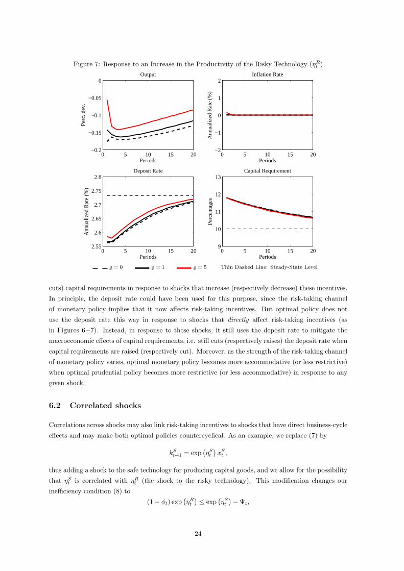
Figure 7: Response to an Increase in the Productivity of the Risky Technology (ηRt )
0 5 10 15 20−0.2
−0.15
−0.1
−0.05
0Output
Periods
Per
c. d
ev.
0 5 10 15 20−2
−1
0
1
2Inflation Rate
Periods
Ann
ualiz
ed R
ate
(%)
0 5 10 15 202.55
2.6
2.65
2.7
2.75
2.8Deposit Rate
Periods
Ann
ualiz
ed R
ate
(%)
0 5 10 15 209
10
11
12
13Capital Requirement
Periods
Per
cent
ages
% = 0 % = 1 % = 5 Thin Dashed Line: Steady-State Level
cuts) capital requirements in response to shocks that increase (respectively decrease) these incentives.
In principle, the deposit rate could have been used for this purpose, since the risk-taking channel
of monetary policy implies that it now affects risk-taking incentives. But optimal policy does not
use the deposit rate this way in response to shocks that directly affect risk-taking incentives (as
in Figures 6−7). Instead, in response to these shocks, it still uses the deposit rate to mitigate the
macroeconomic effects of capital requirements, i.e. still cuts (respectively raises) the deposit rate when
capital requirements are raised (respectively cut). Moreover, as the strength of the risk-taking channel
of monetary policy varies, optimal monetary policy becomes more accommodative (or less restrictive)
when optimal prudential policy becomes more restrictive (or less accommodative) in response to any
given shock.
6.2 Correlated shocks
Correlations across shocks may also link risk-taking incentives to shocks that have direct business-cycle
effects and may make both optimal policies countercyclical. As an example, we replace (7) by
kSt+1 = exp(ηSt)xSt ,
thus adding a shock to the safe technology for producing capital goods, and we allow for the possibility
that ηSt is correlated with ηRt (the shock to the risky technology). This modification changes our
inefficiency condition (8) to
(1− φt) exp(ηRt)≤ exp
(ηSt)−Ψt,
24
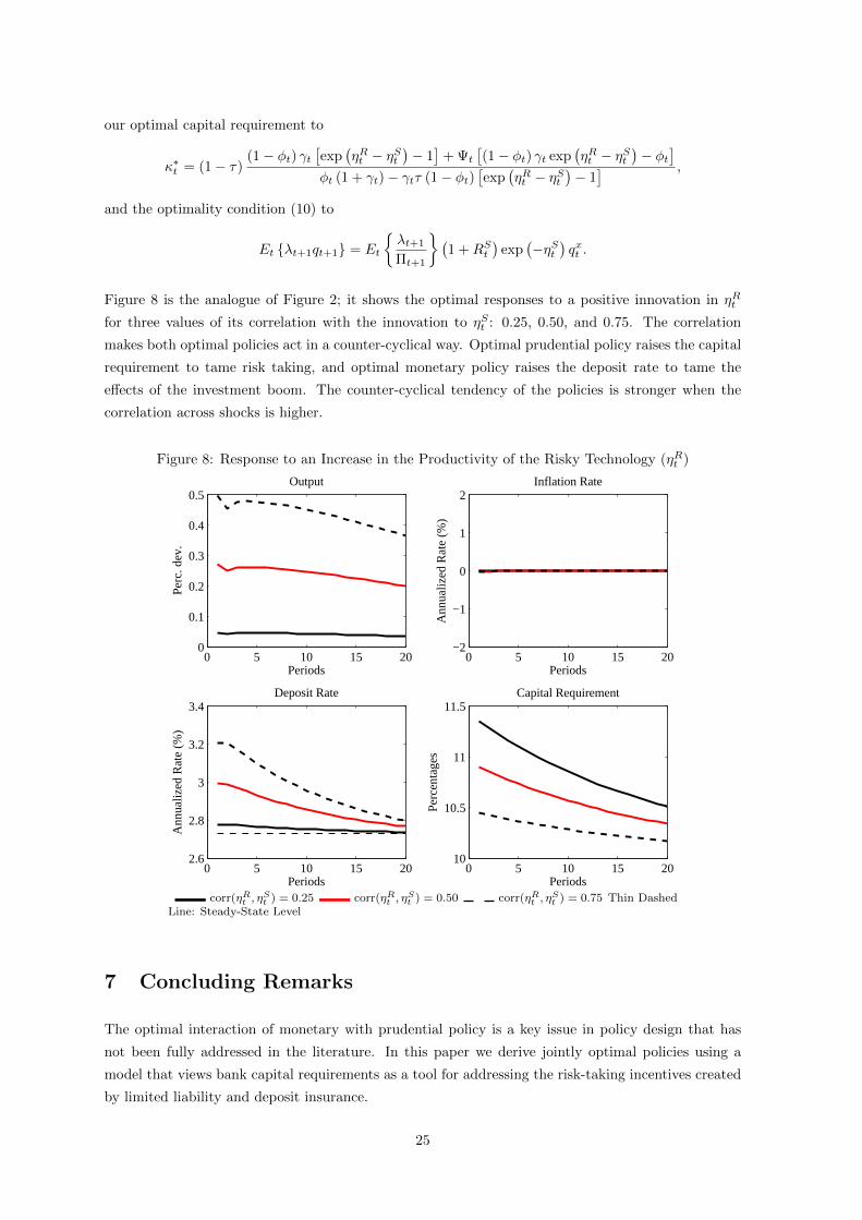
our optimal capital requirement to
κ∗t = (1− τ)(1− φt) γt
[exp
(ηRt − ηSt
)− 1]
+ Ψt
[(1− φt) γt exp
(ηRt − ηSt
)− φt
]φt (1 + γt)− γtτ (1− φt)
[exp
(ηRt − ηSt
)− 1] ,
and the optimality condition (10) to
Et {λt+1qt+1} = Et
{λt+1
Πt+1
}(1 +RSt
)exp
(−ηSt
)qxt .
Figure 8 is the analogue of Figure 2; it shows the optimal responses to a positive innovation in ηRt
for three values of its correlation with the innovation to ηSt : 0.25, 0.50, and 0.75. The correlation
makes both optimal policies act in a counter-cyclical way. Optimal prudential policy raises the capital
requirement to tame risk taking, and optimal monetary policy raises the deposit rate to tame the
effects of the investment boom. The counter-cyclical tendency of the policies is stronger when the
correlation across shocks is higher.
Figure 8: Response to an Increase in the Productivity of the Risky Technology (ηRt )
0 5 10 15 200
0.1
0.2
0.3
0.4
0.5Output
Periods
Per
c. d
ev.
0 5 10 15 20−2
−1
0
1
2Inflation Rate
Periods
Ann
ualiz
ed R
ate
(%)
0 5 10 15 202.6
2.8
3
3.2
3.4Deposit Rate
Periods
Ann
ualiz
ed R
ate
(%)
0 5 10 15 2010
10.5
11
11.5Capital Requirement
Periods
Per
cent
ages
corr(ηRt , ηSt ) = 0.25 corr(ηRt , η
St ) = 0.50 corr(ηRt , η
St ) = 0.75 Thin Dashed
Line: Steady-State Level
7 Concluding Remarks
The optimal interaction of monetary with prudential policy is a key issue in policy design that has
not been fully addressed in the literature. In this paper we derive jointly optimal policies using a
model that views bank capital requirements as a tool for addressing the risk-taking incentives created
by limited liability and deposit insurance.
25

Our benchmark model with perfectly competitive banks and constant marginal costs leads to a simple
optimal assignment of tasks to prudential and monetary policies. The locally optimal mandate of
prudential policy is to ensure that banks never fund inefficient risky projects, but to accomplish this
objective with minimal damage in terms of increased bank lending rates and decreased capital stock.
The distortion is minimized if capital requirements are state dependent. The interaction across policies
then boils down to cutting (raising) interest rates to moderate the contractions (expansions) caused
by changes in the capital requirement. The model also serves to illustrate how time variation in the
capital requirement may be in response to shocks that affect the relative attractiveness of risky and
safe projects.
The extension with an externality in the cost of banking, however, illustrates that optimal policy
interactions may be more complex. In this example, an increase in the aggregate volume of safe
loans increases the costs of originating and monitoring safe loans. This feature, which gives rise to a
risk-taking channel of monetary policy, matters for the optimal policy interactions. In particular, it
makes both policy instruments countercylical under optimal policy in response to certain shocks (like
productivity shocks). However, it does not affect the main implications of the benchmark model for
the optimal policy responses to shocks that directly affect risk-taking incentives: in responses to these
shocks, prudential policy should still be used to tame risk-taking incentives (including those created
by monetary policy when it is accommodative) and monetary policy to mitigate the macroeconomic
effects of prudential policy.
Our model takes deposit insurance as an institutional feature that does not have to be rationalized
within the model.30 The other institutional feature is our assumption that a tax distortion makes
equity finance more expensive than debt finance. We are not aware of any arguments for claiming that
this is a feature of optimal policy in some expanded framework. To the contrary, existing discussions
of this tax distortion [e.g., Admati et al. (2011), Mooij and Devereux (2011)] note its prevalence in
OECD countries and call for removing it. Our motivation for including this policy-induced distortion
in our model is this prevalence and the fact that central banks and prudential regulators cannot change
the tax code.31 We think this tax distortion merits more attention in models of how the banking sector
matters for monetary-policy analysis.32
30Presenting an expanded model in which deposit insurance is optimal (rather than taking it as an exogenous feature)seemed too much of a digression to us, but we could motivate deposit insurance as usual [e.g., following Angeloni andFaia (2011)] in terms of ruling out equilibria with bank runs.
31Besides, under an arbitrarily small tax distortion, all our analytical results (from Proposition 1 to Proposition 6)still hold, as banks still prefer debt finance to equity finance, though the condition stated in Proposition 5 (the “if”part of this proposition) may not be met. In this case, our model is equivalent, at the first order, to a model in whichthe preference for debt finance would come from the presence of deposits in the utility function (as in Van den Heuvel,2008) with an arbitrarily small weight.
32For one thing, this may account for the fact that banks extend credit using loan contracts in reality, even thoughloan contracts are not optimal according to most formal models (with the notable exception of models with costly stateverification).
26
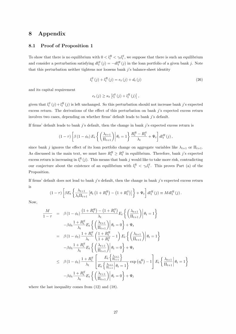
8 Appendix
8.1 Proof of Proposition 1
To show that there is no equilibrium with 0 < lRt < γtlSt , we suppose that there is such an equilibrium
and consider a perturbation satisfying dlSt (j) = −dlRt (j) in the loan portfolio of a given bank j. Note
that this perturbation neither tightens nor loosens bank j’s balance-sheet identity
lSt (j) + lRt (j) = et (j) + dt (j) (26)
and its capital requirement
et (j) ≥ κt[lSt (j) + lRt (j)
],
given that lSt (j)+ lRt (j) is left unchanged. So this perturbation should not increase bank j’s expected
excess return. The derivations of the effect of this perturbation on bank j’s expected excess return
involves two cases, depending on whether firms’ default leads to bank j’s default.
If firms’ default leads to bank j’s default, then the change in bank j’s expected excess return is
(1− τ)
[β (1− φt)Et
{(λt+1
Πt+1
)∣∣∣∣ θt = 1
}RRt −RSt
λt+ Ψt
]dlRt (j) ,
since bank j ignores the effect of its loan portfolio change on aggregate variables like λt+1 or Πt+1.
As discussed in the main text, we must have RRt ≥ RSt in equilibrium. Therefore, bank j’s expected
excess return is increasing in lRt (j). This means that bank j would like to take more risk, contradicting
our conjecture about the existence of an equilibrium with lRt < γtlSt . This proves Part (a) of the
Proposition.
If firms’ default does not lead to bank j’s default, then the change in bank j’s expected excess return
is
(1− τ)
[βEt
{λt+1
λtΠt+1
[θt(1 +RRt
)−(1 +RSt
)]}+ Ψt
]dlRt (j) ≡MdlRt (j) .
Now,
M
1− τ= β (1− φt)
(1 +RRt
)−(1 +RSt
)λt
Et
{(λt+1
Πt+1
)∣∣∣∣ θt = 1
}−βφt
1 +RStλt
Et
{(λt+1
Πt+1
)∣∣∣∣ θt = 0
}+ Ψt
= β (1− φt)1 +RStλt
(1 +RRt1 +RSt
− 1
)Et
{(λt+1
Πt+1
)∣∣∣∣ θt = 1
}−βφt
1 +RStλt
Et
{(λt+1
Πt+1
)∣∣∣∣ θt = 0
}+ Ψt
≤ β (1− φt)1 +RStλt
Et
{λt+1
Πt+1
}Et
{λt+1
Πt+1
∣∣∣ θt = 1} exp
(ηRt)− 1
Et{ λt+1
Πt+1
∣∣∣∣ θt = 1
}
−βφt1 +RStλt
Et
{(λt+1
Πt+1
)∣∣∣∣ θt = 0
}+ Ψl
where the last inequality comes from (12) and (18).
27
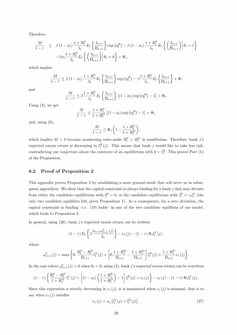
Therefore,
M
1− τ≤ β (1− φt)
1 +RStλt
Et
{λt+1
Πt+1
}exp
(ηRt)− β (1− φt)
1 +RStλt
Et
{(λt+1
Πt+1
)∣∣∣∣ θt = 1
}−βφt
1 +RStλt
Et
{(λt+1
Πt+1
)∣∣∣∣ θt = 0
}+ Ψt,
which implies
M
1− τ≤ β (1− φt)
1 +RStλt
Et
{λt+1
Πt+1
}exp
(ηRt)− β 1 +RSt
λtEt
{λt+1
Πt+1
}+ Ψl
andM
1− τ≤ β 1 +RSt
λtEt
{λt+1
Πt+1
}[(1− φt) exp
(ηRt)− 1]
+ Ψl.
Using (3), we getM
1− τ≤ 1 +RSt
1 +RDt
[(1− φt) exp
(ηRt)− 1]
+ Ψl.
and, using (8),M
1− τ≤ Ψt
(1− 1 +RSt
1 +RDt
),
which implies M < 0 because monitoring costs make RSt > RDt in equilibrium. Therefore, bank j’s
expected excess return is decreasing in lRt (j). This means that bank j would like to take less risk,
contradicting our conjecture about the existence of an equilibrium with 0 < lRt . This proves Part (b)
of the Proposition.
8.2 Proof of Proposition 2
This appendix proves Proposition 2 by establishing a more general result that will serve us in subse-
quent appendices. We show that the capital constraint is always binding for a bank j that may deviate
from either the candidate equilibrium with lRt = 0, or the candidate equilibrium with lRt = γtlSt (the
only two candidate equilibria left, given Proposition 1). As a consequence, for a zero deviation, the
capital constraint is binding –i.e. (19) holds– in any of the two candidate equilibria of our model,
which leads to Proposition 2.
In general, using (26), bank j’s expected excess return can be written
(1− τ)Et
{βλt+1ω
bt+1 (j)
λt
}− et (j)− (1− τ) Ψtl
St (j) ,
where
ωbt+1 (j) = max
{0,RSt −RDt
Πt+1lSt (j) +
[θt
1 +RRtΠt+1
− 1 +RDtΠt+1
]lRt (j) +
1 +RDtΠt+1
et (j)
}.
In the case where ωbt+1 (j) > 0 when θt = 0, using (3), bank j’s expected excess return can be rewritten
(1− τ)
{RSt −RDt1 +RDt
lSt (j) +
[(1− φt)
(1 +RRt1 +RDt
)− 1
]lRt (j) + et (j)
}− et (j)− (1− τ) Ψtl
St (j) .
Since this expression is strictly decreasing in et (j), it is maximized when et (j) is minimal, that is to
say when et (j) satisfies
et (j) = κt[lSt (j) + lRt (j)
]. (27)
28

In the alternative case where ωbt+1 (j) = 0 when θt = 0, consider first the candidate equilibrium with
lRt = 0. Bank j’s expected excess return can then be written
(1− τ) (1− φt){RSt −RDt1 +RDt
lSt (j) +
[1 +RRt1 +RDt
− 1
]lRt (j) + et (j)
}− et (j)− (1− τ) Ψtl
St (j) .
Since this expression is strictly decreasing in et (j), it is maximized for et (j) given by (27). Consider
next the candidate equilibrium with lRt = γtlSt . Bank j’s expected excess return can then be written
(1− τ) (1− φt)β
λtEt
{λt+1
Πt+1
∣∣∣∣ θt = 1
}[(RSt −RDt
)lSt (j) +
(RRt −RDt
)lRt (j)
+(1 +RDt
)et (j)
]− et (j)− (1− τ) Ψtl
St (j) .
This expression is strictly decreasing in et (j), since its derivative with respect to et (j) is strictly
negative:
(1− τ) (1− φt)β
λtEt
{λt+1
Πt+1
∣∣∣∣ θt = 1
}(1 +RDt
)− 1
= (1− τ) (1− φt)Et {λt+1qt+1| θt = 1}
Et {λt+1qt+1}exp
(ηRt) 1 +RSt
1 +RRt− 1
< (1− τ) (1− φt) exp(ηRt) 1 +RSt
1 +RRt− 1
< (1− τ) (1−Ψt)1 +RSt1 +RRt
− 1
< 0,
where the equality comes from (12) and (3), the first inequality from (18), the second inequality from
(8), and the third inequality from the fact that RRt > RSt in equilibrium. Therefore, bank j will
choose the minimal capital requirement, i.e. et (j) satisfying (27). To sum up, the capital constraint
is always binding for a bank j that may deviate from either the candidate equilibrium with lRt = 0,
or the candidate equilibrium with lRt = γtlSt . In particular, for a zero deviation, the capital constraint
is binding –i.e. (19) holds– in any of the two candidate equilibria of our model. This establishes
Proposition 2.
8.3 Proof of Proposition 3
Consider a bank j that takes the maximum amount of risk by setting lRt (j) = γtlSt (j). Using (26)
and (27) to eliminate dt (j) from
ωbt+1 (j) = max
{0,
1 +RStΠt+1
lSt (j) + θt1 +RRtΠt+1
lRt (j)− 1 +RDtΠt+1
dt (j)
},
it is straightforward to show that this bank remains solvent (ωbt+1 (j) > 0) when risky projects fail
(θt = 0) if and only if (21) holds. Part (a) of Proposition 3 follows.
Then, consider a candidate equilibrium with lRt = 0. Using (13) to eliminate dt and (19) to eliminate
et, the representative bank’s expected excess return can be rewritten
(1− τ)Et
{βλt+1ω
bt+1
λt
}− [κt + (1− τ) Ψt] l
St ,
where
ωbt+1 =
[RSt −RDt
Πt+1+
1 +RDtΠt+1
κt
]lSt .
29
The representative bank chooses lSt so as to maximize its expected excess return. Using (3), the
first-order condition of this programme can be written
(1− τ)RSt −RDt1 +RDt
− τκt − (1− τ) Ψt = 0. (28)
We can then use this first-order condition to rewrite κ(RDt , R
St
), at the candidate equilibrium with
lRt = 0, as (20). Parts (b) and (c) of Proposition 3 follow.
8.4 Proof of Proposition 4
To prove Part (a) of Proposition 4, we look for a necessary and sufficient condition on policy instru-
ments for the existence of an equilibrium with lRt = 0. This amounts to looking for a necessary and
sufficient condition on policy instruments for the demand and supply curves on the risky-loans market
to intersect at one or several points(RRt , l
Rt
)with RRt ≥ 0 and lRt = 0. We proceed in several steps.
Step 1: condition for zero demand for risky loans. Given capital producers’ programme, the
portion of the demand curve that is consistent with lRt = 0 is characterized by
1 +RRt1 +RSt
≥ Et {λt+1qt+1| θt = 1}Et {λt+1qt+1}
Et
{λt+1
Πt+1
}Et
{λt+1
Πt+1
∣∣∣ θt = 1} exp
(ηRt)
.
Because θt is independent of any other shock and because the realization of θt does not affect the
aggregate outcome when lRt = 0, the latter inequality can be rewritten
1 +RRt1 +RSt
≥ exp(ηRt)
. (29)
Step 2: condition for zero supply of risky loans. The portion of the supply curve that is
consistent with lRt = 0 can be characterized by a necessary and sufficient condition for an individual
bank j not to deviate from the candidate equilibrium with lRt = 0. We now look for such a condition.
Appendix 8.1 implies that, if some deviations are profitable, then the most profitable deviation is
lRt (j) = γtlSt (j). If bank j makes this deviation, then, using (26) to eliminate dt (j) and (27) to
eliminate et (j), its expected excess return can be rewritten
(1− τ)Et
{βλt+1ω
bt+1 (j)
λt
}− [κt (1 + γt) + (1− τ) Ψt] l
St (j) ,
where
ωbt+1 (j) = max
{0,
[RSt −RDt
Πt+1+ θtγt
1 +RRtΠt+1
− γt1 +RDtΠt+1
+1 +RDtΠt+1
κt (1 + γt)
]lSt (j)
}.
Because θt is independent of any other shock and because the realization of θt does not affect the
aggregate outcome in equilibrium (given that lRt = 0), bank j’s expected excess return can be rewritten,
using (3),
(1− τ)Et
{max
{0,
[RSt −RDt1 +RDt
+ θtγt1 +RRt1 +RDt
− γt + κt (1 + γt)
]lSt (j)
}}− [κt (1 + γt) + (1− τ) Ψt] l
St (j) .
30

Note that the ‘max’ that features in this expression is strictly higher than zero when θt = 1, because
both RRt and RSt are strictly higher than RDt in equilibrium. So we will have to consider two cases,
depending on whether this ‘max’ is strictly higher than zero or equal to zero when θt = 0.
In the case where this ‘max’ is strictly higher than zero when θt = 0, that is to say in the case where
κt > κt, we know from Proposition 1 that bank j’s deviation is not profitable.
In the alternative case where the ‘max’ is equal to zero when θt = 0, that is to say in the case where
κt ≤ κt, bank j’s expected excess return is{(1− τ) (1− φt)
[RSt −RDt1 +RDt
+ γt1 +RRt1 +RDt
− γt + κt (1 + γt)
]− κt (1 + γt)− (1− τ) Ψt
}lSt (j) .
Using (28) to eliminate RSt , we can then rewrite bank j’s expected excess return as{(1− τ) (1− φt) γt
RRt −RDt1 +RDt
− [φt (1 + γt) + γtτ (1− φt)]κt − φt (1− τ) Ψt
}lSt (j) .
Therefore, a necessary and sufficient condition for the deviation not to be profitable is then
[φt (1 + γt) + γtτ (1− φt)]κt + φt (1− τ) Ψt ≥ (1− τ) (1− φt) γtRRt −RDt1 +RDt
. (30)
To sum up, the portion of the supply curve that is consistent with lRt = 0 is characterized by the
condition that either κt > κt, or κt ≤ κt and (30) holds.
Step 3: condition for zero risky loans in equilibrium. The demand and supply curves on the
risky-loans market intersect at one or several points(RRt , l
Rt
)with RRt ≥ 0 and lRt = 0 if and only if
either (i) κt > κt, or (ii) κt ≤ κt, and (30) holds when (29) holds with equality.
Note that, if (29) holds with equality, then, using (28), we can rewrite (30) as
κt ≥ κ∗t ≡ (1− τ)(1− φt) γt
[exp
(ηRt)− 1]
+ Ψt
[(1− φt) γt exp
(ηRt)− φt
]φt (1 + γt)− γtτ (1− φt)
[exp
(ηRt)− 1] , (31)
since the denominator on the right-hand side of this inequality is strictly positive:
φt (1 + γt)− γtτ (1− φt)[exp
(ηRt)− 1]
= φt [1 + γt (1− τ)] + γtτ − γtτ (1− φt) exp(ηRt)
> φt [1 + γt (1− τ)] + γtτΨt
> 0,
where the last but one inequality comes from (8). As a consequence, a necessary and sufficient
condition on policy instruments for the existence of an equilibrium with lRt = 0 is that either κt > κt,
or κ∗t ≤ κt ≤ κt. This condition can be equivalently rewritten κt ≥ min {κt, κ∗t }. Now, using (8) to
replace (1− φt) exp(ηRt)
by 1−Ψt on the right-hand side of (31), we get
κ∗t ≤ (1− τ)−γtΨ2
t + φt (γt −Ψt)
γtτΨt + φt (1 + γt − γtτ)
= κt
{1− γtΨt
γt −Ψt
γtτ + Ψt (1 + γt) (1− τ)
γtΨtτ + φt (1 + γt − γtτ)
}< κt,
31
where the last inequality comes from our assumption that γt > Ψt. Therefore, a necessary and
sufficient condition on policy instruments for the existence of an equilibrium with lRt = 0 is simply
κt ≥ κ∗t . Parts (a) and (b) of Proposition 4 follow.
Finally, Part (c) of Proposition 4 follows straightforwardly from the fact that the denominator on the
right-hand side of (31) is strictly positive, as shown above.
8.5 Proof of Proposition 5
Define welfare as the representative household’s expected utility at date 0, E0
∑∞t=0 β
t U(ct, ht). For
any policy(RDτ , κτ
)τ≥0
, define the distance from(RD∗τ , κ∗τ
)τ≥0
as
ε ≡ max
[maxτ≥0
(∣∣RDτ −RD∗τ ∣∣) ,maxτ≥0
(|κτ − κ∗τ |)]
.
Let us first compare(RD∗τ , κ∗τ
)τ≥0
to policies(RDτ , κτ
)τ≥0
such that ε is arbitrarily small and ∃t ≥ 0,
κt < κ∗t . Moving from(RD∗τ , κ∗τ
)τ≥0
to any such policy triggers a discontinuous increase in the amount
of risk, as it makes banks’ risky loans lRt move from 0 to γtlSt > 0 at some date t ≥ 0. Under our
assumptions (inefficiency condition (8), risk aversion, and no correlation between θt and other shocks),
this discontinuous increase in the amount of risk has a discontinuous negative effect on welfare. Any
other effect on welfare is continuous and, therefore, dominated by this discontinuous negative effect
provided that ε is small enough. As a consequence, welfare is strictly higher under(RD∗τ , κ∗τ
)τ≥0
than
under any such policy provided that ε is small enough.
Let us then compare(RD∗τ , κ∗τ
)τ≥0
to policies(RDτ , κτ
)τ≥0
such that ε is arbitrarily small, ∀τ ≥ 0,
κτ ≥ κ∗τ , and ∃t ≥ 0, κt > κ∗t . Using the equilibrium conditions that are independent of policies,
rewrite welfare as
W[(RDτ)τ≥0
, (κτ )τ≥0 , H0
],
where H0 captures initial conditions (endogenous variables until date −1, exogenous shocks until date
0). Since(RD∗τ
)τ≥0
is the monetary policy that is Ramsey-optimal when (κτ )τ≥0 = (κ∗τ )τ≥0, we have
∀t ≥ 0,∂W
∂RDt
[(RD∗τ
)τ≥0
, (κ∗τ )τ≥0 , H0
]= 0.
Therefore, the first-order Taylor approximation of W[(RDτ)τ≥0
, (κτ )τ≥0 , H0
]in a neighborhood of[(
RD∗τ)τ≥0
, (κ∗τ )τ≥0 , H0
]such that ∀τ ≥ 0, κτ ≥ κ∗τ , is
W[(RDτ)τ≥0
, (κτ )τ≥0 , H0
]= W
[(RD∗τ
)τ≥0
, (κ∗τ )τ≥0 , H0
]+∑+∞
t=0
∂W
∂κt
[(RD∗τ
)τ≥0
, (κ∗τ )τ≥0 , H0
](κt − κ∗t ) +O
(ε2)
,
where ∂W∂κt
is the right derivative of welfare with respect to κt and O(ε2)
is a term of second order in
ε. As a consequence, if
∀t ≥ 0,∂W
∂κt
[(RD∗τ
)τ≥0
, (κ∗τ )τ≥0 , H0
]< 0,
then welfare is strictly higher under(RD∗τ , κ∗τ
)τ≥0
than under any policy(RDτ , κτ
)τ≥0
such that
∀τ ≥ 0, κτ ≥ κ∗τ and ∃t ≥ 0, κt > κ∗t , provided that ε is small enough. Proposition 5 follows.
32

8.6 Proof of Proposition 6
Using (28) and (29), it is easy to show that, at any candidate equilibrium with lRt = 0, the prudential-
policy rule (24) implies (i) κt ≥ κ∗t and (ii) κt = κ∗t if and only if (29) holds with equality. Therefore,
given Proposition 4, there exists a unique equilibrium with lRt = 0 under (24) and, at this equilibrium,
κt = κ∗t and (29) holds with equality.
We now show that there exists no equilibrium with lRt = γtlSt under (24). To that aim, consider a
candidate equilibrium with lRt = γtlSt . Proposition 1 implies that, if ωbt+1 > 0 when θt = 0, then this
candidate equilibrium is not an equilibrium. We focus therefore on the case where ωbt+1 = 0 when
θt = 0. Consider a given bank j, whose expected excess return is
Et
{βλt+1 (1− τ)ωbt+1 (j)
λt
}− et (j)− (1− τ) Ψtl
St (j) ,
where
ωbt+1 (j) = max
{0,
1 +RStΠt+1
lSt (j) + θt1 +RRtΠt+1
lRt (j)− 1 +RDtΠt+1
dt (j)
}.
Using (26) to eliminate dt (j) and (27) to eliminate et (j), its expected excess return can be rewritten
Et
{βλt+1 (1− τ)ωbt+1 (j)
λt
}− κt
[lSt (j) + lRt (j)
]− (1− τ) Ψtl
St (j) ,
where
ωbt+1 (j) = max
{0,
1 +RStΠt+1
lSt (j) + θt1 +RRtΠt+1
lRt (j)− 1 +RDtΠt+1
(1− κt)[lSt (j) + lRt (j)
]}.
If bank j does not deviate from the candidate equilibrium with lRt = γtlSt , then its expected excess
return is equal to[(1− φt)β
(1− τ)[(
1 +RSt)
+ γt(1 +RRt
)− (1 + γt) (1− κt)
(1 +RDt
)]λt
Et
{λt+1
Πt+1
∣∣∣∣ θt = 1
}− κt (1 + γt)− (1− τ) Ψt
]1
1 + γtlt (j) ,
where lt (j) ≡ lSt (j) + lRt (j), since ωbt+1 (j) = 0 when θt = 0. Appendix 8.1 implies that, if some
deviations from the candidate equilibrium with lRt = γtlSt are profitable, then the most profitable
deviation is to provide zero risky loans. If bank j makes this deviation, then its expected excess
return becomes[φtβ
(1− τ)[(RSt −RDt
)+ κt
(1 +RDt
)]λt
Et
{λt+1
Πt+1
∣∣∣∣ θt = 0
}
+ (1− φt)β(1− τ)
[(RSt −RDt
)+ κt
(1 +RDt
)]λt
Et
{λt+1
Πt+1
∣∣∣∣ θt = 1
}− κt − (1− τ) Ψt
]lt (j) .
The change in bank j’s expected excess return, from lRt (j) = γtlSt (j) to lRt (j) = 0, is[
φtβ(1− τ)
[(RSt −RDt
)+ κt
(1 +RDt
)]λt
Et
{λt+1
Πt+1
∣∣∣∣ θt = 0
}− (1− φt)β
(1− τ)
λt
γt1 + γt
(RRt −RSt
)Et
{λt+1
Πt+1
∣∣∣∣ θt = 1
}− (1− τ)
γt1 + γt
Ψt
]lt (j) .
33

It is easy to show that this change is strictly positive, and therefore that bank j gains from deviating
from the candidate equilibrium with lRt = γtlSt , if and only if
κt > −RSt −RDt
1 +RDt+
γt1 + γt
(1− φt)βRRt −R
St
λtEt
{λt+1
Πt+1
∣∣∣ θt = 1}
+ Ψt
φtβ(1+RDt )
λtEt
{λt+1
Πt+1
∣∣∣ θt = 0}
≡ κ
(RDt , R
St , R
Rt , λt,
λt+1
Πt+1, φt
).
Therefore, there exists no equilibrium with lRt = γtlSt under the prudential-policy rule (24) if
κ∗(RDt , R
St , R
Rt , φt
)> κ
(RDt , R
St , R
Rt , λt,
λt+1
Πt+1, φt
),
where κ∗(RDt , R
St , R
Rt , φt
)is the expression on the right-hand side of (24). Using (3), the latter
inequality is easily shown to be equivalent to
1− φtφ2t
Et
{λt+1
Πt+1
}Et
{λt+1
Πt+1
∣∣∣ θt = 0}1−
Et
{λt+1
Πt+1
∣∣∣ θt = 1}
Et
{λt+1
Πt+1
}(RRt −RSt
1 +RDt+ Ψt
)> 0
and is therefore satisfied, given (23) and RRt ≥ RSt . This establishes Proposition 6.
34
References
[1] Admati, Anat R., Peter M. DeMarzo, Martin F. Hellwig, and Paul Pfleiderer (2011), “Fallacies,
Irrelevant Facts, and Myths in Capital Regulation: Why Bank Equity is Not Expensive,” mimeo.
[2] Altunbas, Yener, Leonardo Gambacorta, and David Marques-Ibanez (2010), “Does Monetary
Policy Affect Bank Risk-Taking?,” BIS Working Paper No. 298.
[3] Angeloni, Ignazio, and Ester Faia (2013), “Capital Regulation and Monetary Policy with Fragile
Banks,” Journal of Monetary Economics, 60(3): 311-324.
[4] Basel Committee on Banking Supervision (2010), “Basel III: A Global Regulatory Framework
for More Rresilient Banks and Banking Systems,” Bank for International Settlements.
[5] Benes, Jaromir, and Michael Kumhof (2012), “Risky Bank Lending and Optimal Capital Ade-
quacy Regulation,” mimeo.
[6] Benigno, Pierpaolo and Michael Woodford (2006), “Optimal Taxation in an RBC Model: A
Linear-Quadratic Approach,” Journal of Economic Dynamics and Control, 30(9-10): 1445-1489.
[7] Benigno, Pierpaolo and Michael Woodford (2012), “Linear-quadratic Approximation of Optimal
Policy Problems,” Journal of Economic Theory, 147(1): 1-42.
[8] Benigno, Gianluca, Huigang Chen, Christopher Otrok, Alessandro Rebucci, and Eric Young
(2011), “Monetary and Macro-Prudential Policies: An Integrated Analysis,” mimeo.
[9] Bernanke, Ben (2011), “The Effects of the Great Recession on Central Bank Doctrine and Prac-
tice,” Remarks at the Federal Reserve Bank of Boston 56th Economic Conference, Boston, MA,
October.
[10] Bianchi, Javier (2011),“Overborrowing and Systemic Externalities in the Business Cycle,” Amer-
ican Economic Review, 101(7): 3400-3426.
[11] Bianchi, Javier, and Enrique Mendoza (2011), “Overborrowing, Financial Crises and ‘Macropru-
dential’ Policy,” IMF Working Paper 11/24.
[12] Bils, Mark, and Peter J. Klenow (2004), “Some Evidence on the Importance of Sticky Prices,”
Journal of Political Economy, 112(5): 947-985.
[13] Blanchard, Olivier, Giovanni Dell’Ariccia, and Paolo Mauro (2010), “Rethinking Macroeconomic
Policy,” Journal of Money, Credit and Banking, 42: 199-215.
[14] Borio, Claudio, and Haibin Zhu (2008), “Capital Regulation, Risk-Taking and Monetary Policy:
A Missing Link in the Transmission Mechanism?,” BIS Working Paper No. 268.
[15] Canuto, Otaviano (2011), “How Complementary Are Prudential Regulation and Monetary Pol-
icy?,” Economic Premise No. 60.
[16] Cecchetti, Stephen G., and Marion Kohler (2012), “When Capital Adequacy and Interest Rate
Policy Are Substitutes (and When They Are Not),” BIS Working Paper No. 379.
35
[17] Christensen, Ian, Cesaire Meh, and Kevin Moran (2011) “Bank Leverage Regulation and Macroe-
conomic Dynamics,” mimeo.
[18] Committee on International Economic Policy and Reform (2011), “Rethinking Central Banking,”
Brookings Institution report.
[19] Covas, Francisco, and Shigeru Fujita (2010), “Procyclicality of Capital Requirements in a General
Equilibrium Model of Liquidity Dependence,” International Journal of Central Banking, 6(4):
137-173.
[20] Curdia, Vasco, and Michael Woodford (2009), “Conventional and Unconventional Monetary Pol-
icy,” mimeo.
[21] De Paoli, Bianca, and Matthias Paustian (2013), “Coordinating Monetary and Macroprudential
Policies,” Federal Reserve Bank of New York Staff Report No. 653.
[22] Freixas, Xavier, and Jean-Charles Rochet (2008), Microeconomics of Banking, Second Edition,
Cambridge, MA: MIT Press.
[23] Gete, Pedro, and Natalie Tiernan (2011), “Lax Lending Standards and Capital Requirements,”
mimeo.
[24] Golosov, Mikhail, and Robert E. Lucas Jr. (2007), “Menu Costs and Phillips Curves,” Journal
of Political Economy, 115(2): 171-199.
[25] Hachem, Kinda (2010), “Screening, Lending Intensity, and the Aggregate Response to a Bank
Tax,” mimeo.
[26] Ioannidou, Vasso P., Steven Ongena and Jose Luis Peydro-Alcalde (2009), “Monetary Policy,
Risk-Taking, and Pricing: Evidence from a Quasi-Natural Experiment,” mimeo.
[27] Jeanne, Olivier, and Anton Korinek (2010), “Excessive Volatility in Capital Flows: A Pigouvian
Taxation Approach,” American Economic Review, 100(2): 403-407.
[28] Jermann, Urban, and Vincenzo Quadrini (2009), “Financial Innovations and Macroeconomic
Volatility,” mimeo.
[29] Jermann, Urban, and Vincenzo Quadrini (2012), “Macroeconomic Effects of Financial Shocks,”
American Economic Review, 102(1): 238-271.
[30] Jimenez, Gabriel, Steven Ongena, Jose Luis Peydro-Alcalde, and Jesus Saurina (2012), “Credit
Supply and Monetary Policy: Identifying the Bank Balance-Sheet Channel with Loan Applica-
tions,” American Economic Review 102, 2301–2326.
[31] Kashyap, Anil, Richard Berner, and Charles Goodhart (2011), “The Macroprudential Toolkit,”
Chicago Booth Working Paper No. 11-02.
[32] Levin, Andrew, and David Lopez-Salido (2004), “Optimal Monetary Policy with Endogenous
Capital Accumulation,” mimeo.
[33] Levin, Andrew, Alexei Onatski, John Williams, and Noah Williams (2005), “Monetary Policy un-
der Uncertainty in Microfounded Macroeconometric Models,” in: NBER Macroeconomics Annual
2005, Gertler, M., Rogoff, K., eds, Cambridge, MA: MIT Press.
36

[34] Loisel, Olivier (2014), “Discussion of ‘Monetary and Macroprudential Policy in an Estimated
DSGE Model of the Euro Area’,” International Journal of Central Banking, forthcoming.
[35] Macklem, Tiff (2011), “Mitigating Systemic Risk and the Role of Central Banks,” speech to
Conference de Montreal, Montreal, Quebec, June 6.
[36] Martinez-Miera, David, and Javier Suarez (2012), “A Macroeconomic Model of Endogenous
Systemic Risk Taking,” mimeo.
[37] Mooij, Ruud, and Michael Devereux (2011), “An Applied Analysis of ACE and CBIT Reforms
in the EU,” International Tax and Public Finance, 18(1): 93-120.
[38] Schularick, Moritz, and Alan M. Taylor (2012), “Credit Booms Gone Bust: Monetary Policy,
Leverage Cycles, and Financial Crises, 1870-2008,” American Economic Review, 102(2): 1029-
1061.
[39] Smets, Franck (2013), “Financial Stability and Monetary Policy: How Closely Interlinked?,”
Sveriges Riksbank Economic Review, 2013(3): 121-160.
[40] Svensson, Lars E.O. (2010), “Inflation Targeting and Financial Stability,” policy lecture at the
CEPR/ESI 14th Annual Conference on “How Has Our View of Central Banking Changed with
the Recent Financial Crisis?” hosted by the Central Bank of Turkey, Izmir.
[41] Van den Heuvel, Skander J. (2008), “The Welfare Cost of Bank Capital Requirements,” Journal
of Monetary Economics, 55: 298-320.
[42] Wolf, Martin (2012), “After the Bonfire of the Verities,” Financial Times, May 1.
[43] Yellen, Janet (2010), “Macroprudential Supervision and Monetary Policy in the Post-Crisis
World,” speech at the Annual Meeting of the National Association for Business Economics,
Denver, CO, October 11.
37