Optimal execution using passive and aggressive …tjaisson/Report_Cheuvreux.pdf · Rapport de stage...
51
Transcript of Optimal execution using passive and aggressive …tjaisson/Report_Cheuvreux.pdf · Rapport de stage...

Master 2 - Probabilité et Finance
Promotion 2011-2012
Thibault JAISSON
Rapport de stage de �n d'année
Optimal execution using passive andaggressive orders
Non con�dentiel
Option: Mathématiques Appliquées
Directeur du Master:
Gilles PAGES (LPMA)Correspondant du Master:
Jean-Pierre INDJEHAGOPIAN (ESSEC)
Tuteur de stage:
Charles-Albert LEHALLE (Cheuvreux - Crédit Agricole)
Dates du stage: 01/06/2012 à 01/11/2012
Nom et adresse de l'organisme:
Equipe de Recherche QuantitativeCheuvreux - Crédit Agricole9 Quai Paul Doumer92920 Paris la DéfenseFrance


Résumé:
Ce travail présente un prolongement de la stratégie de liquidation optimale utilisant desordres limites proposée par Guéant, Lehalle et Fernandez dans [9]. Nous proposons ici uneméthode pour incorporer des ordres de marché dans cette stratégie de façon cohérente avecAlmgren Chriss [13]. A partir de notre modèle, nous obtenons une équation de contrôlestochastique proche de celles obtenues dans les deux articles précédents et nous proposons uneheuristique pour avoir une approximation de la solution de cette équation. Ceci nous permetd'obtenir une stratégie implémentable de liquidation optimale.
Abstract:
This work presents a way to prolong the optimal liquidation strategy using limit ordersproposed by Guéant, Lehalle and Fernandez in [9]. We propose a method that allows usto use market orders as well as limit orders in a coherent way with Almgren Chriss [13].From the obtained model, we derive a classical stochastic control equation that looks likethose obtained in the previous frameworks. We propose a heuristic that allows us to have anapproached solution to this equation and we use this solution as an implementable liquidationstrategy.
2


Thanks:I would like like to thank all of the Cheuvreux quantitative research team for welcoming
me during those �ve months. Minh Dang, Vincent Leclerq and Silviu Vlasceanu for their dailyhelp. Joaquin Fernandez, Weibing Huang, George Azevedo, Mathieu Lasnier, Hamza Hartiand Olivier Gueant for all the discussions during which we shared our views of the marketmicro structure.
Most of all, I would like to thank my internship supervisor Charles-Albert Lehalle for histime, his trust and everything that I learned from him.
Ce que j'aime dans les mathématiques
appliquées, c'est qu'elles ont pour
ambition de donner du monde des
systèmes une représentation qui
permette de comprendre et d'agir. Et,
de toutes les représentations, la
représentation mathématique,
lorsqu'elle est possible, est celle qui est
la plus souple et la meilleure. Du coup,
ce qui m'intéresse, c'est de savoir
jusqu'où on peut aller dans ce domaine
de la modélisation des systèmes, c'est
d'atteindre les limites.
Jacques-Louis Lions
4


Contents
1 Introduction 8
1.1 Modern �nancial markets . . . . . . . . . . . . . . . . . . . . . . . . . . . . . . 81.2 Brokerage . . . . . . . . . . . . . . . . . . . . . . . . . . . . . . . . . . . . . . . 81.3 Fast review of the existing models . . . . . . . . . . . . . . . . . . . . . . . . . . 81.4 Presentation of this work . . . . . . . . . . . . . . . . . . . . . . . . . . . . . . . 8
2 Presentation of the articles 9
2.1 The Almgren Chris framework . . . . . . . . . . . . . . . . . . . . . . . . . . . 92.2 The Avellaneda Stoikov framework . . . . . . . . . . . . . . . . . . . . . . . . . 11
3 Aggressive Liquidity-Execution of limit orders 12
3.1 Order intensity . . . . . . . . . . . . . . . . . . . . . . . . . . . . . . . . . . . . 123.2 Characteristic scale . . . . . . . . . . . . . . . . . . . . . . . . . . . . . . . . . . 153.3 In�uence of market conditions . . . . . . . . . . . . . . . . . . . . . . . . . . . . 153.4 In�uence of market states . . . . . . . . . . . . . . . . . . . . . . . . . . . . . . 173.5 Probability of a volume being executed . . . . . . . . . . . . . . . . . . . . . . . 183.6 Conclusion for positive deltas . . . . . . . . . . . . . . . . . . . . . . . . . . . . 19
4 Passive Liquidity-Execution of market orders 19
4.1 Link between the passive and the aggressive liquidity . . . . . . . . . . . . . . . 194.2 Estimation of the available liquidity . . . . . . . . . . . . . . . . . . . . . . . . 204.3 Estimation of the resilience time scale . . . . . . . . . . . . . . . . . . . . . . . 244.4 Conclusion for negative deltas . . . . . . . . . . . . . . . . . . . . . . . . . . . . 26
5 The issue of correlation between orders and price move 27
5.1 A simple model . . . . . . . . . . . . . . . . . . . . . . . . . . . . . . . . . . . . 275.2 Philosophy on which model to choose . . . . . . . . . . . . . . . . . . . . . . . . 285.3 Empirical ex post gains . . . . . . . . . . . . . . . . . . . . . . . . . . . . . . . 285.4 The problem of priority and volume . . . . . . . . . . . . . . . . . . . . . . . . 31
6 The resolution of our problem 35
6.1 The possible intensity for a given cost . . . . . . . . . . . . . . . . . . . . . . . 366.2 The stochastic control problem . . . . . . . . . . . . . . . . . . . . . . . . . . . 386.3 Heuristic . . . . . . . . . . . . . . . . . . . . . . . . . . . . . . . . . . . . . . . . 38
7 Conclusion 39
A Evolution of the order book 40
B Market state estimators 42
C Order arrival intensity in di�erent market states 44
D Liquidity in di�erent market states 47
6


1 Introduction
1.1 Modern �nancial markets
Over the last few years, algorithmic trading has appeared in all the major stock markets andhas taken the place of human operators negotiating prices. This transition has been very fast,some would say too fast and has brought many changes in �nancial markets.
The most famous and controversial of these changes has been the appearance of highfrequency traders whose "usefulness" is still being questioned ([11]). On the one hand, theyclaim to be bringing liquidity to the market but on the other hand, they are accused of makingthe markets unstable. During the Flash Crash that happened on the 6th of May 2010, one ofthe world's most important index the Dow Jones lost up to 9.2% for a few minutes ([1]).
Moreover, new regulations in the United States (Reg NMS in 2005) and in Europe (MiFIDin 2007 and MiFID2 in 2012) have modi�ed the structure of �nancial markets by allowingoperators to trade on stock exchanges other than the primary. This has made markets morecompetitive but it has also brought complexity to the information that market agents get.
For this work, the market can be seen as an order book where agents can either bringliquidity using limit orders or consume liquidity using market orders in what is called a "con-tinuous auction". At each time, two prices are important: the ask price which is the lowestprice at which limit orders are willing to sell stocks and the bid price which is the highestprice at which limit orders are willing to buy stocks (Cf. appendix A for more details on theoperation of order books).
1.2 Brokerage
Cheuvreux, where I spent my end of year internship, is a brokerage �rm. Its main job is toexecute the buying and selling of �nancial securities. In order to do this job as optimallyas possible, it is paramount to understand both the price dynamics at small and large timescales and the relationship between orders and prices. It is also necessary to adapt one'sexecution to the evolution of �nancial markets and to use all the tools available. On thepurely mathematical side, a vast range of articles and models have appeared over the last fewyears to tackle this problem of optimal execution.
1.3 Fast review of the existing models
This literature is often rooted to the seminal papers by Almgren and Chriss, [13] and [12],which introduced an execution cost function that prompts agents to spread their executionswhile their risk aversion spurs them to trade fast. Another family of models appeared followinga paper by Obizhaeva and Wang [2]. These models linked the execution cost in Almgren Chrissto the order book dynamic and its resilience. The third family of models applied to optimalexecution which is being developed by Gueant, Lehalle and Fernandez ([9]) uses the AvellanedaStoikov framework introduced in [6] which models the execution of limit orders.
1.4 Presentation of this work
The goal of this work was to propose a framework that allows to compute optimal executionsstrategies using both market orders and limit orders.
8
• In section 2, we will present more precisely how the Algren-Chriss and the Avellaneda-Stoikov frameworks are applied to optimal execution.
• In section 3, we will study the shape of the market orders arrival intensity function andthe in�uence of the market state on this function.
• In section 4, we will study the shape of the available liquidity in the order book and linkit to the execution cost of the Almgren Chriss framework.
• In section 5, we will see that for passive execution, it is not su�cient to know the orderarrival intensity function but it is also necessary to know the "ex post gain" of one'slimit order. We will study this ex post gain as a function of the priority and of thevolume of the order.
• In section 6, we will regroup our results in a global framework that gives an equationthat looks like those obtained in the Algrem-Chriss or the Avellaneda-Stoikov frameworksand we will propose a heuristic that gives an approximated solution to the equation thatallows us to have a usable optimal execution strategy.
2 Presentation of the articles
In this section, we will present two complementary frameworks that are used to derive execu-tion strategies:
• The Almgren Chris framework which is adapted to aggressive (that is using marketorders) executions.
• The Avellaneda Stoikov framework which is adapted to passive (that is using limit orders)executions.
2.1 The Almgren Chris framework
Here, we brie�y present a framework introduced by Almgren and Chriss in [13] that modelsthe aggressive execution cost (a more precise but harder to use model for liquidity consumingorders is presented in [2]).
2.1.1 The discrete model
In the discrete Almgren Chriss framework, the execution time: [0, T ] is divided into n slicesof time ∆ = T
n . On each slice, the broker decides which quantity nk he wants to execute.The discrete Almgren Chriss model says that the price follows a discrete random walk
modi�ed by an impact function:
Sk = Sk−1 + σ√
∆ζk − g(nkVk )∆
Where Vk is the market volume executed during the kth slice.Moreover, the broker needs to pay an additional cost relatively to the price and thus on
the kth slice he sells at:
S∗k = Sk−1 − h(nkVk )
9

Figure 1: Execution pro�les for di�erent λ
Thus for a given trajectory, we can derive the corresponding expectation and variance ofthe obtained cash X =
∑nk=0 nkS
∗k after our execution.
E[X] = QS0 −∑n
k=0 g(nkVk )xk∆−∑n
k=0 nkh(nkVk )
V aR[X] = σ2∑n
k=0 x2k∆
With xk = Q−∑k
i=0 ni.The broker then needs to optimise a certain criterion. One criterion that is often used in
the Almgren Chriss framework is the mean variance which is parametrised by a risk aversionparameter λ:
(nk) = argmin(nk)[−E(X) + λV aR(X)]
We usually neglect the impact function and we take a linear execution cost:
h( nV ) = εsgn(n) + ηnV
Which gives an explicit execution pro�le (quantity remaining to be executed as a functionof the time): 1.
xk = Q0sinh(κ(T−tk))sinh(κT ) with κ '
√V λσ2
η
2.1.2 The continuous model
When the size of the slice becomes in�nitesimal, the previous model has an obvious continuouslimit:
The broker's control variable becomes his �ow: Φbrokert .
The price dynamic becomes:
10

dSt = σdWt − g(Φbrokert
Φmarkett)dt
The broker's cash becomes:
X0 = 0 and dXt = (St − h(Φbrokert
Φmarkett))Φbroker
t dt
And his quantity of shares:
Q0 = Q and dQt = −Φbrokert dt
The optimal execution problem becomes a classical stochastic control problem whoseHamilton-Jacobi-Bellman equation is (if you neglect the permanent market impact term):
∂tu+ 12∂
2ssu+ supΦΦ[(s− h( Φ
Φmarket))∂u∂x −
∂u∂q ] = 0
And the �nal conditions depend on the broker's utility. An example, which is usually used,is the CARA utility function:
u(t = T, x, q, s) = −e−γ(x+q(s−b))
We will come back in the last section to the resolution of this equation.
2.2 The Avellaneda Stoikov framework
Here, we brie�y present a framework that models the execution of passive orders that hasbeen introduced for market making by Avellaneda and Stoikov in [6] and has been applied topassive execution by Gueant, Lehalle and Fernandez in [9].
2.2.1 The model
In the Avellaneda Stoikov model, the price follows a Brownian motion:
dSt = σdWt
As before, the broker has to liquidate a portfolio of Q shares but to do that, he will uselimit orders. At each time he posts a limit order at a distance δat above the price. His numberof shares follows: qt = Q − Na
t with Na being a jump process counting the shares he sold(that is the number of market orders that arrived at a distance δa from the price).
The arrival rate λa(δa) (intensity of Na) is function of the distance δa.We can parametrise the order arrival intensity with two parameters (A, k):
λa(δa) = Ae−kδa
2.2.2 Implied strategies
This is another classical stochastic control problem whose Hamilton-Jacobi-Bellman equationis:
∂tu(t, x, q, s) + 12∂
2ssu(t, x, q, s) + supδλ(δ)[u(t, x+ s+ δ, q − 1, s)− u(t, x, q, s)] = 0
As in the continuous Almgren Chriss framework, we take the terminal condition:
11

u(t = T, x, q, s) = −e−γ(x+q(s−b))
This equation and the associated optimal strategies have been studied in [9] and [8].Let us notice that if you modify the model, saying that market orders are no longer
Poisson processes but a deterministic �ux of intensity λ(δ); thus neglecting the non executionrisk relatively to the price move risk, the equation becomes:
∂tu(t, x, q, s) + 12∂
2ssu(t, x, q, s) + supδλ(δ)[(s+ δ)∂xu(t, x, q, s)− ∂qu(t, x, q, s)] = 0
Which can be rewritten by inverting λ and by controlling the executed �ux instead of thedistance at which it is executed:
∂tu(t, x, q, s) + 12∂
2ssu(t, x, q, s) + supΦΦ[(s+ λ−1(Φ))∂xu(t, x, q, s)− ∂qu(t, x, q, s)] = 0
That is an Almgren Chriss equation if you take: λ(x) = h−1(−x).The two models are therefore very similar and their associated strategies consist in �nding
an equilibrium between executing rapidly the portfolio because of the risk aversion and exe-cuting slowly the portfolio because of the execution cost which is increasing with the execution�ow. In each case, the important parameter of the model is this execution cost function ofthe �ow or its reverse, the �ow function of the execution cost which is minus the ex post gain.
3 Aggressive Liquidity-Execution of limit orders
In this section, we study the market �ow of market orders. We will use this study to see howmuch execution �ow we can execute by posting limit orders.
3.1 Order intensity
For each time scale dt: 5, 10, 20 and 60 seconds, we part the day in slices of dt we look atthe initial best prices (ie for ask orders the ask price and for bid orders the bid price) and theinitial best opposites (ie for ask orders the bid price and for bid orders the ask price) at thebeginning of each slice. For each distance between 1 and 10 ticks, we see if there has been anask (resp. bid) order above (resp. below) the corresponding price and we look at the volumeof the order. We deduce from this "the order arrival intensity as a function of the distance tothe best initial and to the best opposite initial" by averaging the volumes on all the slices ona month.
Here is the order arrival intensity on both sides for TOTF in January 2012, the cumulativeintensity (if an order executes our passive order, he would also execute it at a better price)and the logarithm of the cumulative intensity: 2, 3.
We observe that log(λ(δ)) = f(δ) is a straight line whose parameters can be estimated bylinear regression so that as it is stated in the articles, for a �xed time scale dt, the cumulativeintensity is close to:
λ(δ) = Ae− δδ0
12

Figure 2: In blue the intensity of the ask orders for di�erent dt 0 being the best ask price atthe beginning of the slice. In red the intensity of the ask orders for di�erent dt 0 being thebest bid price at the beginning of the slice.
Figure 3: In blue the intensity of the ask orders for dt=10, 0 being the best bid price at thebeginning of the slice. In red the intensity of the ask orders for dt=10, 0 being the best askprice at the beginning of the slice.
13

Stocks Volatility Spread Aask Abid deltaask deltabid
OREP.PA 0.18694 2.6334 8.946 8.1637 1.6427 1.583
TECF.PA 0.23371 3.0939 8.9476 8.2107 1.36 1.4511
EDF.PA 0.24388 2.0457 22.5047 21.7054 1.1199 1.3396
ALUA.PA 0.4348 1.5364 220.6533 210.5711 0.90798 0.93425
BNPP.PA 0.46059 3.3992 81.9802 78.033 2.1573 2.329
LAFP.PA 0.33103 3.3667 17.1431 16.626 1.5373 1.6835
PEUP.PA 0.41815 2.3031 36.2664 34.7064 1.2258 1.2876
VIV.PA 0.24973 1.5496 54.9929 55.4095 0.9405 0.95055
BOUY.PA 0.26043 2.4223 15.5085 15.911 1.3557 1.5758
SCHN.PA 0.30457 3.1104 24.0735 23.1785 2.0437 2.1688
SASY.PA 0.19026 1.7277 34.3234 32.1909 1.1405 1.0922
TOTF.PA 0.19166 1.9897 63.4935 63.8952 1.2959 1.3844
RENA.PA 0.3875 1.637 20.9417 19.9111 1.976 1.7681
STM.PA 0.19357 5.5253 48.1054 46.6732 1.7971 1.8158
CNAT.PA 0.45061 2.7577 57.6839 55.8276 1.5329 1.5793
SGOB.PA 0.3022 3.1251 27.5391 25.8593 1.6848 1.6936
ESSI.PA 0.14651 2.3584 5.5801 6.0002 1.1293 1.2136
VIE.PA 0.30589 4.3567 49.236 50.2788 1.9749 1.9442
SGEF.PA 0.24477 3.0901 23.0966 21.9045 1.6289 1.7604
UNBP.PA 0.21577 1.7676 4.7078 4.2963 0.881 0.82286
CAGR.PA 0.46806 3.8813 116.1133 121.0649 2.0282 2.1736
ALSO.PA 0.33841 5.0154 28.5891 27.8444 2.0619 1.8117
CAPP.PA 0.27727 2.9963 11.5075 10.6402 1.6792 1.6608
SOGN.PA 0.34874 -3.1317 97.7979 96.7498 1.9051 2.2141
DANO.PA 0.18795 2.6555 20.807 19.6237 1.6309 1.5666
PERP.PA 0.14774 2.4173 7.0305 7.0323 1.3154 1.3589
AXAF.PA 0.43298 1.6145 99.7508 95.6788 1.017 1.0154
VLLP.PA 0.29737 2.9588 7.5356 7.2494 1.3402 1.535
ACCP.PA 0.35085 3.0728 19.0589 17.9061 1.8342 1.5939
GSZ.PA 0.27921 2.1938 43.1126 43.0069 1.0922 1.0737
CARR.PA 0.32695 1.8761 39.7776 39.4569 1.1918 1.2658
MICP.PA 0.31105 3.4331 12.8942 12.3232 1.6958 1.8001
EAD.PA 0.20484 1.4837 22.1294 19.3913 1.4822 1.5354
FTE.PA 0.20622 1.2493 76.2965 79.4367 0.72968 0.78908
AIRP.PA 0.17903 2.9255 9.8051 9.4543 1.6759 1.7122
LVMH.PA 0.23636 1.3756 12.7896 11.7763 0.85745 0.95424
Table 1: Parameters of the order arrival intensity function of the best for stocks of the CAC40in January 2012.
14
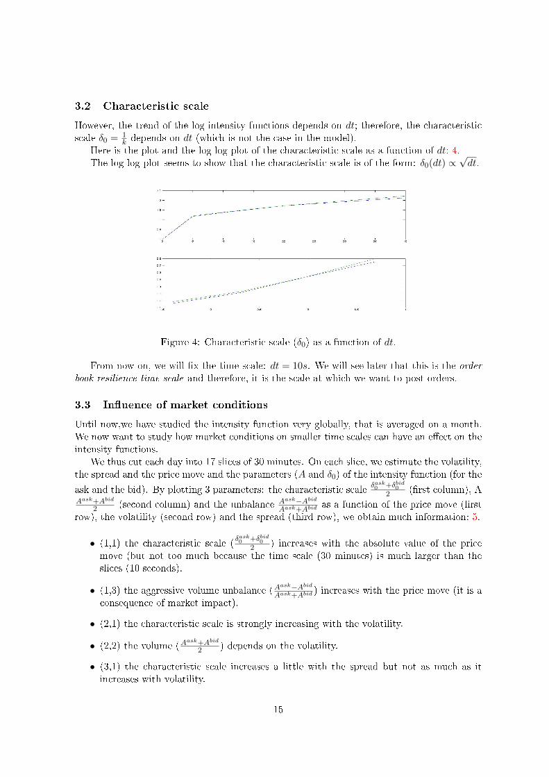
3.2 Characteristic scale
However, the trend of the log-intensity functions depends on dt; therefore, the characteristicscale δ0 = 1
k depends on dt (which is not the case in the model).Here is the plot and the log-log plot of the characteristic scale as a function of dt: 4.The log-log plot seems to show that the characteristic scale is of the form: δ0(dt) ∝
√dt.
Figure 4: Characteristic scale (δ0) as a function of dt.
From now on, we will �x the time scale: dt = 10s. We will see later that this is the orderbook resilience time scale and therefore, it is the scale at which we want to post orders.
3.3 In�uence of market conditions
Until now,we have studied the intensity function very globally, that is averaged on a month.We now want to study how market conditions on smaller time scales can have an e�ect on theintensity functions.
We thus cut each day into 17 slices of 30 minutes. On each slice, we estimate the volatility,the spread and the price move and the parameters (A and δ0) of the intensity function (for the
ask and the bid). By plotting 3 parameters: the characteristic scaleδask0 +δbid0
2 (�rst column), AAask+Abid
2 (second column) and the unbalance Aask−AbidAask+Abid
as a function of the price move (�rstrow), the volatility (second row) and the spread (third row), we obtain much information: 5.
• (1,1) the characteristic scale (δask0 +δbid0
2 ) increases with the absolute value of the pricemove (but not too much because the time scale (30 minutes) is much larger than theslices (10 seconds).
• (1,3) the aggressive volume unbalance (Aask−Abid
Aask+Abid) increases with the price move (it is a
consequence of market impact).
• (2,1) the characteristic scale is strongly increasing with the volatility.
• (2,2) the volume (Aask+Abid
2 ) depends on the volatility.
• (3,1) the characteristic scale increases a little with the spread but not as much as itincreases with volatility.
15
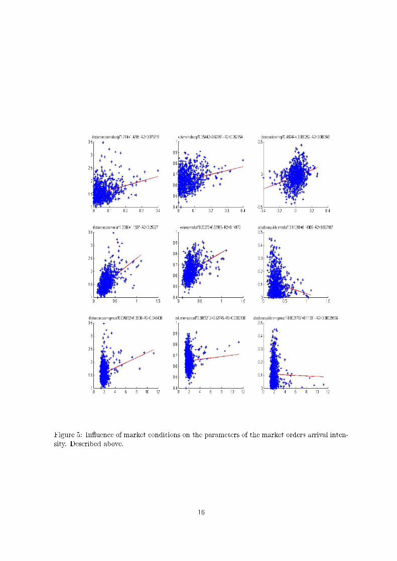
Figure 5: In�uence of market conditions on the parameters of the market orders arrival inten-sity. Described above.
16
Remark: The fact that the best explanatory factor for the characteristic scale δ0 is thevolatility leads us to think that the orders arrival intensity far from the initial price is due toprice moves more than it is due to liquidity arriving far from the actual mid price. We willsee later that this is important.
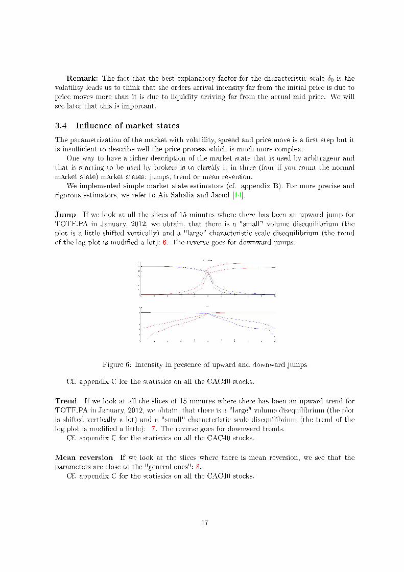
3.4 In�uence of market states
The parametrization of the market with volatility, spread and price move is a �rst step but itis insu�cient to describe well the price process which is much more complex.
One way to have a richer description of the market state that is used by arbitrageur andthat is starting to be used by brokers is to classify it in three (four if you count the normalmarket state) market states: jumps, trend or mean reversion.
We implemented simple market state estimators (cf. appendix B). For more precise andrigorous estimators, we refer to Ait-Sahalia and Jacod [14].
Jump If we look at all the slices of 15 minutes where there has been an upward jump forTOTF.PA in January, 2012, we obtain, that there is a "small" volume disequilibrium (theplot is a little shifted vertically) and a "large" characteristic scale disequilibrium (the trendof the log plot is modi�ed a lot): 6. The reverse goes for downward jumps.
Figure 6: Intensity in presence of upward and downward jumps
Cf. appendix C for the statistics on all the CAC40 stocks.
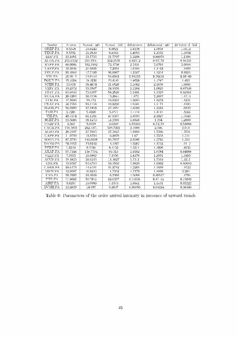
Trend If we look at all the slices of 15 minutes where there has been an upward trend forTOTF.PA in January, 2012, we obtain, that there is a "large" volume disequilibrium (the plotis shifted vertically a lot) and a "small" characteristic scale disequilibrium (the trend of thelog plot is modi�ed a little): 7. The reverse goes for downward trends.
Cf. appendix C for the statistics on all the CAC40 stocks.
Mean reversion If we look at the slices where there is mean reversion, we see that theparameters are close to the "general ones": 8.
Cf. appendix C for the statistics on all the CAC40 stocks.
17

Figure 7: Intensity in presence of upward and downward trends
Figure 8: Intensity in presence of mean reversion
3.5 Probability of a volume being executed
Until now, we only have studied the order arrival intensity as a �ow, taking all the volumethat arrives. From a practical point of view, it is more interesting to study the probabilitythat if you place an order of size V at a certain distance at the beginning of the slice, you willbe executed during the slice.
In order to do that, we proceed like previously except that instead of estimating the orderarrival intensity, we estimate the probability that a volume V will be executed on the slice(for V equal to 1, 10, 50, 100, 1000 or 10000 on TOTF.PA in January 2012): 9.
We observe that like the order arrival intensity, the probability of being executed can bemodelled by:
P = P0e− δδ0
And that δ0 does not depend on the volume.
18

Figure 9: Probability and log-probability of being executed for di�erent volumes (from top tobottom: V equal to 1, 10, 50, 100, 1000 or 10000) for ask and bid orders.
3.6 Conclusion for positive deltas
To conclude this section, let us summarise the most important points of the order arrivalintensity function:
• It is very well approximated by a two parameters function: I(δ) = Ae− δδ0
• A is proportional to the market volume
• δ0 is proportional to the volatility
• Market states can provoke an imbalance between the ask function and the bid function
Remark: Practically, if you need the "local" intensity function you can use the empiricalone on the last hour.
4 Passive Liquidity-Execution of market orders
4.1 Link between the passive and the aggressive liquidity
In the model of Avellaneda Stoikov, the order arrival intensity is de�ned on both sides of thespread. In reality, the nature of the liquidity is very di�erent on both sides of the spread: onthe passive side, the liquidity is a volume while on the aggressive side, the liquidity is a �ow.
One of the main goals of this study was to �nd a coherent way to prolong the aggressive�ow to the passive side. That is to de�ne and estimate the arriving �ow of liquidity on theside where there already is liquidity.
A "natural" idea is that there is an order book resilience time scale after which the aggres-sively consumed liquidity comes back. Therefore, if we make the assumption that this timescale does not depend on the distance to the mid price, then the lambda function (that is
19

a "�ow of arriving liquidity") becomes proportional to the average available liquidity in theorder book. In fact that might be wrong for two reasons:
• The price might not revert back to the initial price.
• The liquidity return time scale might depend on the distance.
A more precise model of the resilience of the price is available in [4] or [3].In fact, the important function is not the order �ow function of the distance but the order
�ow function of the execution cost which is de�ned in Almgren Chriss.To estimate these functions, we need to:
• Estimate the available liquidity.
• Estimate the "resilience time scale" under which the liquidity does not have time tocome back.
4.2 Estimation of the available liquidity
4.2.1 Methodology
We take 39 stocks of the CAC40 on January 2012, as before we cut each day into slices of 30seconds. On each slice, we look at the liquidity as a function of the distance to the best andto the best opposite.
4.2.2 Average results
Here is the average order book and the average cumulated liquidity for TOTF in January, asa function of the distance to the best and to the best opposite: 10, 11.
Figure 10: As a function of the distance to the best (x− axe = 1 corresponds to the best ask,x− axe = 2 corresponds to the second best ask,...; x− axe = −1 corresponds to the best bid,x− axe = −2 corresponds to the second best bid,...)
We parametrise the order book as a linear function up to a point and then a constant. Wethus have two (main) parameters: the slope and the saturation liquidity value Lask and Lbid
(the "increasing scale" dask and dbid is implied as the quotient of those two parameters).
20

Stocks Volatility Spread Lask Lbid dask dbid
AIRP.PA 0.10893 3.8608 913.9625 837.3241 6.5868 6.3845
ALUA.PA 0.42269 1.6421 66548.8063 67998.6284 2.9642 2.9405
AXAF.PA 0.25109 1.5969 12088.9853 12229.9195 2.8713 2.8874
BNPP.PA 0.29622 3.2237 2217.2297 2273.0755 5.3117 5.3479
BOUY.PA 0.19025 2.6084 1927.8293 1990.6009 4.4481 4.3241
CAPP.PA 0.19228 3.9996 827.0927 786.0007 5.9079 5.8238
CARR.PA 0.1895 2.0716 5437.3957 5591.2977 3.7341 3.6419
DANO.PA 0.12494 3.7622 2438.8134 2299.1572 5.4352 5.5393
ESSI.PA 0.095134 3.0597 1186.2224 1048.1174 4.7738 4.8053
FTE.PA 0.12753 1.3083 27769.5941 28135.9251 2.9507 3.0456
OREP.PA 0.13138 2.8418 679.8035 618.6428 4.6312 4.4567
LAFP.PA 0.21023 4.2404 1103.2143 1097.3437 6.2703 6.0253
LVMH.PA 0.1599 1.5819 2019.9496 1959.6957 3.0914 3.2445
MICP.PA 0.22391 3.2841 856.879 831.4592 4.6208 4.6207
CNAT.PA 0.32008 3.336 7375.4784 7365.5918 4.5258 4.5241
PERP.PA 0.11104 2.8898 858.9858 822.2745 4.6813 4.4798
PEUP.PA 0.29758 1.9811 2962.6112 3088.3461 4.2604 3.9238
PRTP.PA 0.18208 1.844 1047.4167 1013.4619 3.2951 3.3655
PUBP.PA 0.14433 3.949 692.4306 709.8882 5.5515 5.5381
RENA.PA 0.25082 5.2881 855.8271 874.2759 7.0936 7.2072
SGOB.PA 0.2032 3.4061 2213.2278 2229.2466 5.4319 5.3992
SCHN.PA 0.19633 4.0792 757.8587 713.8524 6.184 6.2126
SGEF.PA 0.17029 3.6013 2101.7063 1985.8592 5.3912 5.4385
STM.PA 0.36624 5.0165 4920.0374 4674.0785 6.9269 7.0873
SOGN.PA 0.34394 2.6971 4379.3636 4510.1033 4.502 4.4599
TECF.PA 0.18342 4.9623 360.4924 339.9282 6.7673 6.7384
TOTF.PA 0.14417 2.2168 3160.0094 3239.4716 3.987 4.0152
UNBP.PA 0.14337 1.9669 1339.1728 1339.8671 3.4423 3.5604
VLLP.PA 0.17709 5.0683 363.0105 336.6892 6.9342 6.7549
SASY.PA 0.11523 1.8867 2787.1823 2769.798 3.7158 3.7851
EAD.PA 0.16035 3.5765 2011.9558 1928.9244 5.1258 5.4066
VIE.PA 0.23384 2.3302 5834.2775 5791.6698 3.9564 3.9076
VIV.PA 0.20199 1.4449 13218.11 13563.5406 2.9043 2.9083
CAGR.PA 0.31824 3.0443 11971.2213 12207.5419 4.747 4.6811
GSZ.PA 0.17831 2.0863 7720.9877 7777.8695 3.7473 3.8696
ALSO.PA 0.21926 4.4003 1672.7896 1565.095 6.7022 6.6879
EDF.PA 0.16295 2.1908 5035.4498 5067.9543 3.8257 3.7069
SEVI.PA 0.15273 1.7858 5292.9432 5395.0997 3.6614 3.6465
Table 2: Parameters of the average liquidity for the stocks of the CAC40
21

Figure 11: As a function of the distance to the best opposite
Remark: That is a surprisingly good approximation for large tick and small tick assetsalike but only if we consider the volume as a function of the distance to the best opposite (andnot the best).
4.2.3 Dependence of the results to market conditions
Like for the order arrival intensity, we now want to study how market conditions on smallertime scales can have an e�ect on the intensity functions.
We thus cut each day into slices of one hour. On each slice, we estimate the volatility, thespread and the price move and the parameters (L and d) of the intensity function for the ask
and the bid. By plotting 3 parameters: dask+dbid
2 (�rst column), Lask+Lbid
2 (second column)
and Lask−LbidLask+Lbid
as a function of the price move (�rst row), the volatility (second row) and thespread (third row), we obtain much information: 12.
• (1,1) the characteristic scale (dask+dbid
2 ) does not depend on the price move.
• (1,3) the volume unbalance (Lask−Lbid
Lask+Lbid) does not depend on the price move.
• (2,1) the characteristic scale increases with the volatility. It is normal, when the priceis uncertain, people are less willing to place liquidity close to the mid price.
• (2,2) the volume (Lask+Lbid
2 ) decreases with the volatility.
• (3,1) the characteristic scale increases strongly on the spread. It means that it is the"good" liquidity scale.
22

Figure 12: Explanation of the order book by the market conditions
23

4.2.4 Dependence of the results to the market state
As opposed to the order arriving intensity, the market state does not seem to in�uence theliquidity .
Cf. Appendix D for statistics on all the CAC40 stocks.
4.3 Estimation of the resilience time scale
In the Almgren Chriss framework, the volume of one's order impacts his price in two di�erentways:
• By the market impact that has a "long term" e�ect on the price.
• By the execution cost that does not a�ect the market price but a�ects your executionprice.
The execution cost is the most important e�ect on volume when you deal with optimalexecution. It is what will make the broker want to spread his order execution.
It is possible to estimate it by looking at orders globally and looking at the di�erencebetween the executed vwap and the average of the market price during the execution but theresults are very noisy and need a lot of data. Here we propose another method.
4.3.1 Execution costs of the orders in the market
To estimate the execution cost function h(Φbrokert
Φmarkett), we look at all the slices of 5 minutes during
5 months. On each slice, we look at the order unbalance: V ask−V bidV ask+V bid
that we will call period
liquidation ratio (plr) (the plr will estimateΦbrokert
Φmarketton the slice) and the di�erence between
VWAP ask (the average price obtained by ask orders) (resp. VWAP bid) and a reference price
on the slice: P beginning+P end
2 (where P beginning is the last price at the beginning of the sliceand P end is the last price at the end of the slice).
We plot VWAP ask − P beginning+P end
2 as a function of the plr: 13.
Figure 13: Execution cost=h(Φbrokert
Φmarkett)
24

Remark: Taking P beginning+P end
2 as a "reference" price is a classical method to only havethe execution cost and not the market impact in the expectation of the di�erence. We thereforesuppose that: h(plr) = E[VWAP ask − P beginning+P end
2 ]. In order to estimate h, we thus needto know the expectation of the di�erence between the executed price and the reference priceas a function of the plr. To do that, we average the execution cost on slices of plr (slices of5%). A tendency clearly appears: 14.
Figure 14: Execution cost=E[h(Φbrokert
Φmarkett)]
We notice that for small enough plrs, the execution cost seems to be a linear function ofthe plr. That is the form that we will choose for h. We thus proceed with a linear regressionof the execution cost for plrs between -20% and 20% and we get:
ECask = 0.0114× plr + 0.0022
ECbid = 0.0117× plr + 0.0023
4.3.2 Execution cost as the consumption of the order book-Resilience time scale
If you don't introduce an "order book resilience time scale", there is an incoherence betweenthe Almgren Chriss framework (execution cost function of the plr that is a �ow) and theaggressive execution that regularly consumes the order book (execution cost function of thevolume). Indeed, if the resilience was in�nite, one could execute as much volume as one wantsfor a constant execution cost by dividing his execution.
That is why we introduce a time scale under which it is useless to trade because theliquidity has not had time to come back.
If you look at the order book: 15, we notice that for small volumes, the average impact ofan order of volume V in the order book has about the same form as our execution cost.
ExecCost(plr, 5min) = aφ+ bplr and ExecCost(V ) = aφ+ βV
25

Figure 15: Average order book.
If we look at the execution cost in Almgren Chriss as the repetition of order book con-sumption every δt. On a slice of ∆T = 5minutes (n = ∆T
δt ), we have that the execution cost
of the consumption of V∆T
n in the order book must be equal to the execution cost associated
to the corresponding plr ( V ∆T
FlowMarket∆T) estimated earlier thus:
a+ b V ∆T
FlowMarket∆T= a+ β V
∆T
n
Thus we get the resilience time scale which is the scale ∆Tn corresponding to the n that
makes the equality above true:
δtres = bβF lowMarket
For TOTF: β = T ick2V best
= 0.002Tick/Stock, b = 0.0115 = 2.3Tick and FlowMarket =130Stock/Second.
So that:
δtres ' 10sec
Thus, if there is more than 10 seconds between our trades, we can consider that the orderbook is resilient.
4.4 Conclusion for negative deltas
To conclude this section, let us summarise the most important points of the passive liquidityarrival rate:
• It is proportional to the order book, the proportionality constant being a resilience timescale.
• It is very well approximated by a two parameters function: L(δ) = L0min(1, δc )
26

• c is proportional to the spread Φ and L0 is inversely proportional to the spread. There-fore, the cumulated arriving liquidity up to δ is function of δ
Φ . The spread is thereforethe "good" price scale for passive liquidity.
Practically, if you want to know how much liquidity you will be able to consume instanta-neously, you only need to look at the order book but we will see that it is also useful to knowthe average execution cost.
5 The issue of correlation between orders and price move
5.1 A simple model
Let us present a simple model to show the importance of the correlation between orders andprices:
• The mid-price (Pt) is a Brownian motion of volatility σ.
• The spread is constant.
• A limit ask (resp. bid) order is executed if and only if the best ask (resp. bid) goesabove (resp. below) the price of this limit order.
In this model, the probability of being executed at a distance δ from the initial mid-priceduring a slice of length dt is the probability that the maximum of the Brownian motion on[t, t+ dt] is superior to Pt + δ − φ
2 that is:
P (δ, dt) = 2N(− δ−φ2
σ√dt
) with N(x) =∫ x−∞
1√2πe−
t2
2 dt
We take σ = 0.6tick.s−12 which corresponds to 27% and φ = 2ticks.
We see that in this model, we also have a characteristic scale in√dt but the probability
curves do not really look like those of the data: 16.
Figure 16: Probability and log-probability of being executed in the model
27

5.2 Philosophy on which model to choose
Let us remark that this model is deeply di�erent from the Avellaneda Stoikov model. Indeed,in the article, orders and prices are "independent" while here, orders follow prices (or pricesfollow orders). In fact, the truth is probably between those two models: prices and orders arenot independent but "the temporary impact is smaller than the permanent impact" in otherwords, the price is mean-reverting.
Remark: The model of Avellaned Stoikov describes better the probability at a giventime-scale but this model describes better the characteristic scale δ0 as a function of dt.
Example: Let us assume that we are risk neutral and that we can instantaneously sell orbuy at the bid or ask price. To buy an action on a slice dt we will:
• Choose a delta.
• Post a passive order at distance δ of the best bid and if we are not executed, buy at thebest ask at the end of the slice.
Those two models imply di�erent strategies:
• In the model of the article, the optimal δ is: argmax[P (δ, dt)δ] that is δ0.
• In our model, the optimal δ is 1.
This example shows that, in order to choose an optimal delta, it is not su�cient for ourmodel to verify the order arriving statistics, it must also take into account the "ex post gain"of orders if they happen.
For the task at hand, the parameter that will determine which model to choose is thecorrelation between orders and price move. Indeed, the question is:
"If we are executed far from the initial mid-price, are we "very happy" because on average
the price is equal to the mid-price at the beginning of the slice whether or not we are executed
or are we "not so happy" because if we are executed, it means that the price is not as good as
it was at the beginning of the slice?"
In order to answer this question, we plot the expectation of the variation of the priceknowing that there has been an order at distance δ (which will give us the "ex post gain" ofour order).
5.3 Empirical ex post gains
5.3.1 Methodology
As before, we take slices of dt = 10s. At the end of each slice, we look at:
• The best ask and bid to have been executed on the slice minus the initial best ask andbid (δask = askmax− askinit and δbid = bidinit− bidmin)
• The last price P0 at the beginning of the slice (which we will use as a reference price)
• The last price 100 orders after the end of the slice Pf .
For a δ �xed, we de�ne:
28

• The average ex ante gain of an order executed at δ from the initial best price: δ +bestask0 − P0.
• The average permanent market impact of the orders executing an order placed at δ fromthe initial best price: E[Pf − P0|orderδexecuted]. Which is the price ex post after theexecution of the order.
• The average ex post gain of an order placed at δ which is the di�erence between the twoprevious prices.
5.3.2 Results
Small tick stocks: 17 and Large tick stocks: 18. We notice that (column of the right)the ex post gain of limit orders is positive. It means that if one could always have priority,he would win on average and thus have an arbitrage; that is market making. We also notice19 that for stocks with small spread/tick ratios the ex post gain is higher. We will see thatit means that priority becomes more important for these stocks. We also notice that the expost gain does not depend a lot on δ (for δ ≥ 0) while in the Avellaneda Stoikov model, thisex post gain is equal to δ.
Figure 17: Left column: ex ante gain and permanent market impact as a function of δ (forthe bid side and the ask side). Right column: ex post gain as a function of δ. For ACCP.PA,RENA.PA and BNPP.PA
29

Figure 18: Left column: ex ante gain and permanent market impact as a function of δ. Rightcolumn: ex post gain as a function of δ. For ALUA.PA, FTE.PA and LVMH.PA
Figure 19: Ex post gain at the �rst and second limit as a function of the spread/tick ratio.
30

5.4 The problem of priority and volume
In the previous section, we assumed that our limit orders were executed each time a marketorder hit our limit. In fact, in the order book, limit orders are executed by market orders inthe order (ie priority) at which they have been placed, therefore, in function of our priority,we will not always be executed and the less we have priority, the less we will gain if we areexecuted (because if we are executed after a lot of volume, it will mean that the fair price islikely to be "impacted" towards you).
5.4.1 The priority issue
Methodology (very criticizable): We parameter the "priority e�ect" as a probability pof being executed when the best price on the slice is equal (and not superior as before) to thelimit.
Therefore, we take:
ExPostPrice(δ, p) =p(NnExPostPrice(δ,1)−Nδ+TickExPostPrice(δ+T ick,1))+Nδ+TickExPostPrice(δ+T ick,1)
p(Nδ−Nδ+Tick)+Nδ+Tick
As an ex post price knowing that we have been executed at a distance δ from the bestprice with a priority parameter p.
Where: Nδ is the intensity that arrives above δ and PrixExPost(δ, 1) is your ex post priceif you have a priority maximum (that we have estimated earlier).
Ex post gain as a function of the priority: Let us consider TOTF which is a very liquidstock with an average spread/tick ratio. If we plot the ex post gain at the �rst and secondlimit as a function of the priority: 20, we notice that there is a "limit priority" above whichone has a positive average ex post gain.
Figure 20: Ex post gain as a function of the priority at the �rst and second limit
31

Stocks Price ref Tick Spread Ga1 Gb
1 Ga2 Gb
2
OREP.PA 80.93 0.01 2.243 0.56674 0.39598 0.79192 0.22204
TECF.PA 71.94 0.01 2.7275 0.39416 0.37033 -0.0078724 0.47247
EDF.PA 17.83 0.005 1.9246 0.50632 0.79366 -0.69443 0.88638
ALUA.PA 1.37 0.001 1.6657 1.2825 1.0013 0.79147 0.31165
BNPP.PA 32.795 0.005 2.9703 0.43425 0.44887 0.55221 0.59802
LAFP.PA 31.15 0.005 3.2407 -0.1218 -0.065927 -0.092676 0.11075
PEUP.PA 13.34 0.005 2.6002 0.82695 0.38662 1.0652 0.11987
VIV.PA 14.165 0.005 1.4082 1.0792 0.86589 0.84889 -0.35126
BOUY.PA 23.39 0.005 2.0963 0.58763 1.093 0.22471 1.3791
SCHN.PA 45.86 0.005 3.3787 -0.44525 -0.10411 -0.79269 -0.41014
SASY.PA 55.1 0.01 1.5163 0.89577 1.2059 0.72581 1.0822
TOTF.PA 40.225 0.005 1.7463 0.84282 0.89043 0.76769 0.76125
RENA.PA 32.865 0.005 4.0277 -0.64348 -0.46696 -1.0904 -0.0098947
PRTP.PA 119.05 0.05 1.5364 0.98494 1.4904 0.70732 0.75111
STM.PA 5.085 0.001 3.6888 -0.29716 -0.16779 -0.38816 -0.65297
CNAT.PA 2.211 0.001 2.7155 0.7419 0.54185 0.74845 0.97906
SGOB.PA 34.15 0.005 2.8451 0.30133 0.074157 0.52713 0.14685
ESSI.PA 56.18 0.01 2.0936 0.50826 0.72752 0.27552 0.54081
VIE.PA 8.755 0.001 4.7503 -1.2444 -1.1287 -1.6881 -0.77633
SGEF.PA 35.68 0.005 2.8474 0.68412 0.60819 1.0841 0.50233
UNBP.PA 142 0.05 1.6178 0.97419 0.95633 0.2069 0.23561
CAGR.PA 4.611 0.001 3.4639 0.29542 0.13325 0.81469 0.0069123
ALSO.PA 28.53 0.005 3.2898 0.18202 0.21348 0.18433 0.071276
CAPP.PA 28.185 0.005 2.6993 0.033015 0.49979 -0.54905 0.52062
SOGN.PA 20.83 0.005 3.0543 0.74927 0.75112 0.74445 0.70931
DANO.PA 47.42 0.005 2.8801 0.38711 0.84699 0.58807 0.67403
PERP.PA 74 0.01 2.1797 0.63602 0.5442 0.68764 0.5175
AXAF.PA 11.74 0.005 1.4208 1.0003 1.0468 0.93109 0.93136
VLLP.PA 50.53 0.01 2.3553 0.55715 0.21167 0.95116 0.41339
ACCP.PA 23.515 0.005 3.0207 0.019713 0.37557 0.12613 0.34434
GSZ.PA 19.235 0.005 1.6716 1.069 1.0807 1.0612 0.62938
CARR.PA 17.125 0.005 1.8007 0.79157 0.45445 0.4958 0.82188
MICP.PA 51.21 0.01 2.3755 0.18012 0.16648 0.19246 -0.26288
EAD.PA 25.845 0.005 2.3837 0.76246 0.8946 0.63159 0.99034
FTE.PA 11.11 0.005 1.2006 1.3557 1.1951 0.8268 -0.14535
PUBP.PA 38.685 0.005 2.9427 -0.003643 0.50623 0.41577 0.59146
AIRP.PA 94.82 0.01 2.5489 0.67978 0.97086 0.63602 1.46
LVMH.PA 122.85 0.05 1.2995 1.0903 1.3277 0.084578 0.98395
Table 3: Ex post gain as a function of the spread/tick ratio (Gxi ex post gain on the x side atthe ith limit).
32

Priority null: If we have a priority null (p = 0) it means that we are the last to be executedat δ. Here is ex post gain if we are the last to be executed at the �rst and second limits: 21.We notice that the ex post gain is negative but superior to minus a tick.
Figure 21: Ex post gain as a function of the spread/tick ratio for the CAC40 for priority null
Conclusion on the priority issue: We have seen that for a maximum priority, the ex postgain of an order is between 0 and 2bp and for a minimum priority, the ex post gain is between-2bp and 0. Since those values are not too important, we will assume that on average, the expost gain of our (small) orders is zero.
5.4.2 The volume issue-Passive execution cost
We have seen that for the �rst limits, the ex post gain does not depend a lot on how far youare from the best price. Thus, since the execution intensity is higher at the best price, italways seems better to be at the �rst limit. In fact, we have forgotten about the volume issuewhich is close to the priority issue. When we post a lot of volume the end of our volume willhave a lower priority than the beginning of our volume. Thus the ex post gain of our orderwill become negative. To quantify this e�ect, we propose a non arbitrage hypothesis on theshape of the available liquidity.
A model to quantify the passive execution cost: Let us assume that for given marketconditions, on a given slice, the permanent market impact: MIP (V ) = E[∆P last|V ask = V ]does not depend on the passive liquidity that we insert.
We will also use the fact that "if we post a small order at δ above the existing liquidity, wehave an ex post gain null" to obtain a relationship between the permanent market impact andthe available liquidity. This kind of equalities can be "justi�ed" with non arbitrage argumentswhich prolong those of [7] in which the spread is shown to be the average market impact ofan order. We will use them to derive the execution cost as a function of the posted volume.
Let us de�ne the expectation of the price move on the slice knowing that a volume V ofthe order book has been executed during the slice:
C(V ) ≡ E[MIP (V x)|V x ≥ V ]
Using the hypothesis, we know that for V = Liq(δ) (the liquidity available up to (including)δ), C is equal to the price corresponding to δ minus the reference price P0:
33

Stocks Price ref Tick Spread Ga1 Gb
1 Ga2 Gb
2
OREP.PA 80.93 0.01 2.243 -0.26077 -0.6188 -0.067805 -0.98267
TECF.PA 71.94 0.01 2.7275 -0.70376 -0.6712 -1.3364 -0.38045
EDF.PA 17.83 0.005 1.9246 -0.91594 -0.35288 -2.0359 -1.517
ALUA.PA 1.37 0.001 1.6657 0.1026 -0.19356 -1.8208 -1.4305
BNPP.PA 32.795 0.005 2.9703 -0.49146 -0.40337 -0.35506 -0.54308
LAFP.PA 31.15 0.005 3.2407 -1.1089 -0.95042 -1.1183 -0.76736
PEUP.PA 13.34 0.005 2.6002 -0.13093 -0.63131 -0.011479 -1.2472
VIV.PA 14.165 0.005 1.4082 0.078101 -0.48785 -0.79529 -3.1288
BOUY.PA 23.39 0.005 2.0963 -0.4699 0.25898 -1.2636 -0.077746
SCHN.PA 45.86 0.005 3.3787 -1.4596 -1.5575 -1.7008 -1.7388
SASY.PA 55.1 0.01 1.5163 -0.28267 0.077569 -0.79785 -0.25982
TOTF.PA 40.225 0.005 1.7463 -0.06171 -0.12944 -0.33069 -0.32875
RENA.PA 32.865 0.005 4.0277 -1.797 -1.4051 -2.4068 -1.0373
PRTP.PA 119.05 0.05 1.5364 -0.24509 -0.17406 -1.6822 -1.0148
STM.PA 5.085 0.001 3.6888 -1.3802 -1.2188 -1.2731 -2.0832
CNAT.PA 2.211 0.001 2.7155 -0.3967 -0.13773 0.038902 -0.52937
SGOB.PA 34.15 0.005 2.8451 -0.59319 -0.93338 -0.87872 -0.82801
ESSI.PA 56.18 0.01 2.0936 -0.35598 -0.33977 -1.1538 -0.039222
VIE.PA 8.755 0.001 4.7503 -2.5187 -1.8827 -2.5087 -1.5452
SGEF.PA 35.68 0.005 2.8474 -0.061636 -0.30306 0.072638 -0.50545
UNBP.PA 142 0.05 1.6178 -0.40639 0.068036 -2.4975 -2.2679
CAGR.PA 4.611 0.001 3.4639 -0.46344 -0.90192 -0.55229 -0.96826
ALSO.PA 28.53 0.005 3.2898 -0.76141 -0.76042 -0.70668 -1.1154
CAPP.PA 28.185 0.005 2.6993 -1.1571 -0.61222 -1.6653 -0.79682
SOGN.PA 20.83 0.005 3.0543 -0.28233 -0.30438 -0.2788 -0.2513
DANO.PA 47.42 0.005 2.8801 -0.31455 -0.47163 -0.20161 -0.60372
PERP.PA 74 0.01 2.1797 -0.19756 -0.44074 -0.3074 -0.46347
AXAF.PA 11.74 0.005 1.4208 0.015833 0.025405 -0.82376 -0.32509
VLLP.PA 50.53 0.01 2.3553 -0.31887 -0.48605 -0.3766 -0.62826
ACCP.PA 23.515 0.005 3.0207 -0.99041 -0.55451 -0.74756 -0.53464
GSZ.PA 19.235 0.005 1.6716 0.20395 0.081076 -0.34329 -0.71575
CARR.PA 17.125 0.005 1.8007 -0.24885 -0.58921 -0.57648 -0.3698
MICP.PA 51.21 0.01 2.3755 -0.82616 -1.0709 -1.024 -1.3409
EAD.PA 25.845 0.005 2.3837 -0.15789 -0.0023468 -0.75353 -0.30044
FTE.PA 11.11 0.005 1.2006 0.20801 -0.13637 -0.65307 -2.0341
PUBP.PA 38.685 0.005 2.9427 -0.81248 -0.48271 -0.74939 -0.13512
AIRP.PA 94.82 0.01 2.5489 -0.30452 0.016021 -0.68672 -4.0233e-005
LVMH.PA 122.85 0.05 1.2995 -0.17846 0.45726 -2.4918 0.22879
Table 4: Ex post gain as a function of the spread/tick ratio for priority null
34

C(Liq(δ)) = ask + δ − P0
Let us now place an ask order of size v at δ (above Liq(δ)), our ex post gain is:
EPG(δ, v) = ask + δ − P0 − C(Liq(δ) + v) = C(Liq(δ))− C(Liq(δ) + v)
However, C is only de�ned for V = Liq(δ). To compute the ex post gain we will need anadditional assumption:
Example 1: Let us make the assumption that you can post orders wherever you want(tick=0) and that the cumulative liquidity function is of the form (which is the form that wehave seen before 10):
Liq(d) = 1d≥aΦ[α( dΦ − a)2 + V best( dΦ − a)]
Then the function C is known for every V (since the liquidity is continuous) and :
C(V ) = aΦ + ΦV best
2α (√
1 + 4αV
V best2− 1)
And the passive ex post gain of an order of size v placed at d is:
EPG(d, v) = aΦ + ΦV best
2α (√
1 + 4αLiq(d)
V best2− 1)− aΦ− ΦV best
2α (√
1 + 4α(Liq(d)+v)
V best2− 1)
Which we can approximate by:
EPG(d, v) ' Φ vV best
1√1+
4αLiq(d)
V best2
if 4αLiq(d)
V best2is small.
Example 2: If between the Liq(δ)s, we prolong C linearly, if we put v at the δth limit, weget (Vδ = Liq(δ)− Liq(δ − Tick) being the volume in δ):
C(Liq(δ) + v) =v(δ+T ick)+(Vδ+Tick−v)δ
Vδ+TickTick + E[last− ask]
And we have the ex post gain:
EPG(δ, v) = δ − v( δTick
+1)−v δTick
Vδ+TickTick − δ = − v
Vδ+TickTick
6 The resolution of our problem
Until now, we have shown that:
• The execution �ow that you get by placing for δt (10 sec) Vδ (small) at δ is:
λ(δ) = Vδδt P0e
− δδ0
• The ex post gain of this order knowing that it has been executed is:
EPG(δ, v) = C(Liq(δ))− C(Liq(δ) + v)
• The execution cost of your �ow of market orders is:
h(Flow) = Φ(a+ b FlowF lowMarket )
35

6.1 The possible intensity for a given cost
In this subsection, we will see given an arbitrary execution cost c how much �ow we canexecute.
6.1.1 Aggressively
Aggressively, the answer is immediate and given by the cost function h of Almgren Chriss:
Flowag(c) = FlowMarket
b ( cΦ − a)+
6.1.2 Passively
Passively, the question is much more complicated. To answer it, we need to see how muchstocks we can put at each limit so that if it is executed, we get an ex post gain equal to −c.
• At the �rst limit, if one puts v∗1 above the volume that is already there: V1, his ex postgain will be:
EPG(1, v∗1) = Tick × v∗1V2
Thus if you want to have an ex post gain superior to −c, you can put up to v∗1 = V2× cT ick .
• At the second limit, if one puts v∗2 above the volume that is already there: V2 (knowingthat you have already put V ∗1 at the �rst limit), his ex post gain will be:
EPG(2, v∗2) = Tick × v∗1+v∗2V3
Thus if you want to have an ex post gain superior to −c, you can put up to v∗2 =V3 × c
T ick − v∗1.
• By recurrence, we compute the expression of the volume v∗i that you can put at the ith
best price if you want to have an ex post gain superior to −c with:
v∗i = Vi+1 × cT ick −
∑i−1j=1 v
∗j = (Vi+1 − Vi) c
T ick if i ≥ 2.
This will imply an execution �ow function of the execution cost:
Flowpass(c) = c×P0T ick×δt [e
−Tickδ0 V2 +
∑+∞i=2 e
− iT ickδ0 (Vi+1 − Vi)] = K × c
6.1.3 Total �ow
From the two previous paragraph, we get that for a given execution cost c that one is readyto pay, one can have an execution �ow of:
Flow(c) = Flowpass(c) + Flowag(c) = K1 × c+K2 × (c− c0)+
For TOTF.PA, we get: K1 = 2500, K2 = 13000 and c0 = 0.002.
36

Figure 22: Execution �ows as a function of the execution cost.
6.1.4 Example of placement on a slice
To illustrate the work above with an example, let us suppose that at a time t, the order bookis: 24.
Figure 23: Example of the state of the order book at time t.
Let us assume that we have determined (we will see in the next section how) that weshould have an execution cost on slice t of c = 0.7 and that the last price is 99. We derivethat we can:
• Execute aggressively the �rst limit.
• Post 350 at the �rst limit, post 175 at the second limit and post 105 at the third limit.
Figure 24: In red, the liquidity that we consume. In green, the liquidity that we post.
37

6.2 The stochastic control problem
Let us focus on order execution of Q stocks between 0 and T . We look at the order �ow asa continuous deterministic function of the execution cost (or reversely, the execution cost isfunction of the execution �ow).
The Hamilton-Jacobi-Bellman equation to solve thus becomes:
∂tu(t, x, q, s) + 12σ
2∂2ss(t, x, q, s) + supc Flow(c)[(s− c)∂xu(t, x, q, s)− ∂qu(t, x, q, s)] = 0
With �nal conditions which correspond to the CARA function;
u(t = T, x, q, s) = −e−γ(x+q(s−b))
6.3 Heuristic
Instead of resolving exactly this equation (I would not know where to start), we will use aheuristic (that is close to the one presented in [5]) to determine the optimal quote δ∗. Anotheradvantage of using this heuristic will be our ability to take into account the market conditions(expected volatility, volume and spread) in our strategy (an exact resolution wouldn't).
The principle of the heuristic is to say that the strategy (strategy CF for constant �ow)which consists in executing with a constant �ow our inventory is not too far from the optimalstrategy. Following this strategy, we know our �nal expected utility:
uCF (0, 0, Q, S0) ' E[−e−γXCFT ] ' −1 + γ(E[XCF
T ]− γ2V aR[XCF
T ])
Furthermore, we know that for a constant execution:
E[XCFT ] = QS0 −QFlow−1(QT )
V aR[XCFT ] = Q2Tσ2
2
In the same way:
uCF (t, x, q, s) ' −1 + γ(x+ qs− qF low−1( qT−t)−
γ2q2(T−t)σ2
2 )
This is not a good estimation of the expected utility; but in a Hamilton-Jacobi-Bellmanequation, the most important part of the equation is not the solution itself but the criterionthat the resolution gives you to have an optimal strategy.
Here, the criterion to �nd the optimal c which is the control variable is:
c∗(t, x, q, s) = argmaxc(Flow(c)[(s− c)∂xuCF (t, x, q, s)− ∂quCF (t, x, q, s)])
And by taking the u∗ found above, you get the cost c∗ which equilibrates (for your givenrisk aversion λ = γ
2 ) your will to trade fast and avoid the risk and your will to trade slowlyand have a small execution cost. Moreover, for a given c∗, we know how to place your ordersat the beginning of each slice.
Operational remark: In order to estimate the Flow function in the estimation of u, itis better to take the average parameters on long time scales. To estimate the Flow functionin the choice of the optimal c, it is better to use a "local" estimation of the Flow function(actual order book, market state...).
38

7 Conclusion
In Science in general but especially in the study of complex systems such as the dynamicsof an order book, a model is never perfect. The trick is to build a model that takes intoaccount the main stylised facts that intervene in the problem that one is trying to solve. Forthe task at hand of optimal execution, we believe that the two main stylised facts are: theprobability that one order of any kind be executed and the ex post gain (or execution cost) ofthis order. With this in mind, and using the existing literature and market data, we have builta framework that allows us to use both market and limit orders; we have given a mathematicalformulation to the problem and we have proposed a heuristic to have a practical solution tothis problem.
39

A Evolution of the order book
At each time during the day, in an order book, a market participant can see a successionof quotes ( 25) that we call Limit Orders; each limit order is characterised by its price, itsquantity and its side.
Figure 25: A real order book
If the side of the limit order is Ask, it means that the order o�ers to sell up to its quantityat its price; therefore a market participant can buy the quantity using what we call an askMarket Order. If the side of the limit order is Bid, it means that the order o�ers to buy upto its quantity at its price; therefore a market participant can sell the quantity using what wecall a bid Market Order.
Throughout the day, market participants can bring liquidity to the market by posting limitorders or consume liquidity buy using market orders ( 26).
40

Figure 26: A schematic order book
Remark: At each time, any ask order is strictly above any bid order (or else they wouldexecute each other).
This evolution of liquidity is called a Continuous Auction and imply an evolution of thedi�erent important prices:
• The Ask Price, which is the lowest price of an ask limit order.
• The Bid Price, which is the highest price of a bid limit order.
• The Mid Price, which is the average of the ask price and the bid price.
• The Last Price, which is the last price at which there has been a trade (ask or bid).
Two important parameters, of the order book are:
• The Spread denoted Φ which is the di�erence between the ask price and the bid price.It is an excellent explanatory factor when dealing with liquidity issues.
• The Tick Size which is the step at which prices are quoted (limit order cannot be postedat any price).
For a model explaining the evolution of liquidity, see [10].
41

B Market state estimators
Here are the 3 detectors that we use in this work:
• Jump detector: if the price move on one minute is larger than 6 times the standarddeviation expected at the current volatility, there is a jump.
• Trend detector: if the linear regression of the price by the time (on a 15 minutesslice)has a R2 larger than 90%, there is a trend.
• Mean reversion detector: if the di�erence between the maximum and the minimumof the price (on a 15 minutes slice) is smaller than 25% times the standard deviationexpected at the current volatility , there is mean reversion.
Here are three (beautiful) examples of what our estimators detect: 27, 28, 29.
Figure 27: A jump
42

Figure 28: A trend
Figure 29: A mean reversion
43

C Order arrival intensity in di�erent market states
Stocks Anorm Ajump+ask Ajump+bid deltanorm deltajump+ask deltajump+bid
OREP.PA 8.5548 10.4628 7.3794 1.6128 2.2032 1.6399
TECF.PA 8.5791 8.7304 6.6757 1.4055 1.861 1.313
EDF.PA 22.1051 24.8037 19.3521 1.2298 1.7601 1.2676
ALUA.PA 215.6122 229.0936 184.574 0.92112 1.1103 0.72999
BNPP.PA 80.0066 90.7313 71.6046 2.2431 2.4311 2.3073
LAFP.PA 16.8846 19.3509 14.4797 1.6104 1.8014 1.5419
PEUP.PA 35.4864 39.0032 28.9218 1.2567 1.689 0.93916
VIV.PA 55.2012 51.2959 44.3693 0.94553 1.4396 1.0652
BOUY.PA 15.7098 15.3774 14.3793 1.4658 1.368 1.1621
SCHN.PA 23.626 31.6488 25.3262 2.1062 2.3283 1.9587
SASY.PA 33.2572 33.8494 28.2767 1.1164 1.5534 1.0477
TOTF.PA 63.6944 59.7467 57.7153 1.3401 1.9864 1.107
RENA.PA 20.4264 22.2256 20.3835 1.872 2.4093 1.6592
STM.PA 47.3893 50.8837 34.624 1.8065 2.087 1.5647
CNAT.PA 56.7558 67.9962 41.8631 1.5561 1.7474 1.2773
SGOB.PA 26.6992 31.3051 24.4543 1.6892 1.863 1.7447
ESSI.PA 5.7901 5.4422 4.4695 1.1714 0.95485 0.78886
VIE.PA 49.7574 51.5334 42.064 1.9595 2.4382 1.8662
SGEF.PA 22.5006 25.5048 17.6053 1.6946 2.1233 1.4824
UNBP.PA 4.502 4.486 3.3575 0.85193 1.3596 1.2854
CAGR.PA 118.5891 135.9115 131.6463 2.1009 2.616 2.0532
ALSO.PA 28.2167 29.929 25.3866 1.9368 2.9198 1.4569
CAPP.PA 11.0739 13.9427 9.5108 1.67 1.97 1.5506
SOGN.PA 97.2738 148.3952 127.6659 2.0596 2.4746 2.6744
DANO.PA 20.2153 23.5628 20.6984 1.5987 2.1635 1.5067
PERP.PA 7.0314 6.5371 5.4957 1.3371 1.5915 1.1813
AXAF.PA 97.7148 107.3118 90.5894 1.0162 1.144 0.87059
VLLP.PA 7.3925 7.2195 5.7208 1.4376 1.5317 1.3227
ACCP.PA 18.4825 19.8931 15.011 1.7141 2.2999 1.3839
GSZ.PA 43.0597 50.2986 39.221 1.0829 1.9018 1.1829
CARR.PA 39.6173 48.8811 45.2595 1.2288 1.3426 1.4916
MICP.PA 12.6087 13.2865 10.0103 1.7479 2.1574 1.6913
EAD.PA 20.7603 33.1692 22.3752 1.5088 1.9839 1.5722
FTE.PA 77.8666 89.3943 79.9964 0.75938 0.9221 0.93421
AIRP.PA 9.6297 10.6819 7.8209 1.6941 2.8548 1.2523
LVMH.PA 12.2829 17.1385 11.0931 0.90585 1.4138 0.69196
Table 5: Parameters of the order arrival intensity in presence of upward jumps
44
Stocks Anorm Atrend+ask Atrend+bid deltanorm deltatrend+ask deltatrend+bid
OREP.PA 8.5548 10.8443 6.9821 1.6128 1.5858 1.0512
TECF.PA 8.5791 11.2539 6.8363 1.4055 1.3252 1.3554
EDF.PA 22.1051 25.7755 21.7707 1.2298 0.88979 1.1396
ALUA.PA 215.6122 331.1534 222.3555 0.92112 0.95179 0.86131
BNPP.PA 80.0066 102.1882 72.4738 2.2431 2.0704 2.0988
LAFP.PA 16.8846 21.9388 17.2331 1.6104 1.4462 1.1969
PEUP.PA 35.4864 47.7192 36.8067 1.2567 1.1254 0.9265
VIV.PA 55.2012 74.6154 54.6953 0.94553 0.76676 0.66489
BOUY.PA 15.7098 19.7038 22.4747 1.4658 1.7242 1.452
SCHN.PA 23.626 28.4674 21.0528 2.1062 2.1656 1.6805
SASY.PA 33.2572 35.5507 24.9359 1.1164 1.0625 0.67536
TOTF.PA 63.6944 75.6397 58.2529 1.3401 1.1329 0.92161
RENA.PA 20.4264 30.4158 19.2064 1.872 2.2087 1.4513
STM.PA 47.3893 59.472 43.8301 1.8065 1.8272 1.4221
CNAT.PA 56.7558 88.1456 44.3226 1.5561 1.5471 1.4105
SGOB.PA 26.6992 37.8959 27.1834 1.6892 1.5594 1.6822
ESSI.PA 5.7901 5.4366 3.5277 1.1714 1.4747 1.3568
VIE.PA 49.7574 61.1181 47.9357 1.9595 2.1027 1.7043
SGEF.PA 22.5006 28.1473 18.2395 1.6946 1.234 1.2869
UNBP.PA 4.502 5.0339 3.6149 0.85193 0.74179 0.54868
CAGR.PA 118.5891 202.4474 139.7002 2.1009 2.196 2.048
ALSO.PA 28.2167 37.7085 27.5925 1.9368 1.7396 1.7031
CAPP.PA 11.0739 13.8734 10.3979 1.67 1.7558 1.511
SOGN.PA 97.2738 140.0698 95.7857 2.0596 1.5795 1.554
DANO.PA 20.2153 23.6343 14.1267 1.5987 1.4753 1.2117
PERP.PA 7.0314 9.2705 8.1733 1.3371 1.1006 1.4935
AXAF.PA 97.7148 138.7754 93.315 1.0162 1.0284 0.64088
VLLP.PA 7.3925 10.6662 7.1556 1.4376 1.2951 1.3495
ACCP.PA 18.4825 20.6245 14.4027 1.7141 1.7343 1.3211
GSZ.PA 43.0597 54.6784 38.1503 1.0829 1.0302 0.80683
CARR.PA 39.6173 44.6181 31.3782 1.2288 1.1089 1.1022
MICP.PA 12.6087 16.6245 11.7352 1.7479 1.8336 2.205
EAD.PA 20.7603 28.4603 16.2366 1.5088 0.88517 1.4788
FTE.PA 77.8666 90.2815 69.0332 0.75938 0.47155 0.73849
AIRP.PA 9.6297 10.6989 7.1973 1.6941 1.1431 0.92222
LVMH.PA 12.2829 14.987 9.2637 0.90585 0.93224 0.38349
Table 6: Parameters of the order arrival intensity in presence of upward trends
45

Stocks Anorm Amrask Amrbid deltanorm deltamrask deltamrbid
OREP.PA 8.5548 7.7679 6.8291 1.6128 1.4755 1.5315
TECF.PA 8.5791 8.1129 7.0767 1.4055 1.5223 1.1311
EDF.PA 22.1051 21.9601 17.2998 1.2298 0.68979 1.3411
ALUA.PA 215.6122 194.2154 192.4524 0.92112 0.7389 0.72798
BNPP.PA 80.0066 63.6775 58.9788 2.2431 1.9375 2.0147
LAFP.PA 16.8846 13.5682 13.1247 1.6104 1.2534 1.4164
PEUP.PA 35.4864 31.1429 29.8465 1.2567 1.511 1.7096
VIV.PA 55.2012 44.3343 45.5981 0.94553 0.72189 0.84717
BOUY.PA 15.7098 14.8918 14.9223 1.4658 1.679 1.7685
SCHN.PA 23.626 19.7855 18.6198 2.1062 1.8577 1.9246
SASY.PA 33.2572 36.1894 29.9528 1.1164 1.068 1.029
TOTF.PA 63.6944 65.4702 65.1869 1.3401 1.0925 1.2054
RENA.PA 20.4264 16.9643 16.9783 1.872 1.6572 1.3987
STM.PA 47.3893 49.7589 48.7631 1.8065 1.8314 1.3881
CNAT.PA 56.7558 57.035 50.6227 1.5561 1.4604 1.6534
SGOB.PA 26.6992 24.3776 26.0865 1.6892 1.7969 1.3595
ESSI.PA 5.7901 5.5109 5.3565 1.1714 0.87883 1.2583
VIE.PA 49.7574 48.6908 49.2215 1.9595 2.1465 1.9525
SGEF.PA 22.5006 22.2153 22.625 1.6946 1.4173 1.6111
UNBP.PA 4.502 4.8877 3.7871 0.85193 0.7459 0.55555
CAGR.PA 118.5891 98.2128 96.2171 2.1009 1.5324 1.5743
ALSO.PA 28.2167 29.0852 29.249 1.9368 2.0798 1.787
CAPP.PA 11.0739 9.9579 9.508 1.67 1.3598 1.7516
SOGN.PA 97.2738 70.7011 70.3291 2.0596 1.4338 1.836
DANO.PA 20.2153 23.3378 19.0479 1.5987 1.6782 1.5679
PERP.PA 7.0314 7.5117 6.6053 1.3371 1.1636 1.1559
AXAF.PA 97.7148 92.3108 86.8604 1.0162 0.85748 0.87628
VLLP.PA 7.3925 7.1834 5.9221 1.4376 1.2492 1.5366
ACCP.PA 18.4825 18.857 21.1887 1.7141 1.7563 1.3385
GSZ.PA 43.0597 40.5073 41.1951 1.0829 0.83448 1.0083
CARR.PA 39.6173 30.5681 27.7333 1.2288 0.93086 0.75741
MICP.PA 12.6087 12.2012 12.9723 1.7479 1.444 1.7294
EAD.PA 20.7603 18.6068 15.719 1.5088 1.2271 1.0821
FTE.PA 77.8666 74.16 76.9017 0.75938 0.68321 0.68572
AIRP.PA 9.6297 8.7623 8.306 1.6941 1.7541 1.5772
LVMH.PA 12.2829 11.4513 10.2218 0.90585 0.33102 0.6581
Table 7: Parameters of the order arrival intensity in presence of mean reversion
46

D Liquidity in di�erent market states
Stocks Lnorm Lask Lbid dnorm dask dbid
ACCP.PA 1530.8788 1317.9403 1344.1348 5.7164 5.8368 5.8497
AIRP.PA 875.6433 720.7339 562.8203 6.4856 5.5949 6.1355
ALUA.PA 67273.7173 63872.4613 64075.6361 2.9523 2.8772 2.9165
AXAF.PA 12159.4524 10882.3557 10316.6255 2.8794 2.9568 3.1621
BNPP.PA 2245.1526 2084.6413 2049.4449 5.3298 5.4047 5.6531
BOUY.PA 1959.2151 1966.3006 2236.553 4.3861 4.395 4.1459
CAPP.PA 806.5467 700.3735 654.8014 5.8658 6.049 6.0375
CARR.PA 5514.3467 5243.9796 5123.4696 3.688 3.9694 3.9967
DANO.PA 2368.9853 2332.3444 2218.6243 5.4872 3.6139 3.8776
ESSI.PA 1117.1699 1248.4858 1015.9421 4.7896 4.8282 4.9281
FTE.PA 27952.7596 25873.6261 26584.7492 2.9982 3.0655 3.1382
OREP.PA 649.2231 665.3026 608.5672 4.5439 4.5042 4.4955
LAFP.PA 1100.279 1012.1617 1043.7524 6.1478 6.3189 6.1497
LVMH.PA 1989.8226 2006.7391 1849.3935 3.168 3.1726 3.1807
MICP.PA 844.1691 807.2295 864.9917 4.6208 4.6065 4.458
CNAT.PA 7370.5351 6699.1036 5930.4254 4.5249 4.7531 4.6966
PERP.PA 840.6302 885.7757 839.1398 4.5805 4.0122 4.2072
PEUP.PA 3025.4786 2638.1498 2834.5144 4.0921 3.7992 3.743
PRTP.PA 1030.4393 874.1047 984.3108 3.3303 3.3345 3.7237
PUBP.PA 701.1594 688.0773 653.2251 5.5448 5.634 5.703
RENA.PA 865.0515 744.0809 764.4179 7.1504 7.2557 7.4698
SGOB.PA 2221.2372 2129.4888 2122.3827 5.4156 5.2164 5.1201
SCHN.PA 735.8556 814.3963 683.4286 6.1983 6.1652 6.3512
SGEF.PA 2043.7827 1921.0784 1895.8265 5.4149 5.2769 5.3813
STM.PA 4797.0579 4556.1281 4399.6209 7.0071 7.8883 7.3998
SOGN.PA 4444.7334 4049.8651 4225.2578 4.4809 4.4182 4.4652
TECF.PA 350.2103 368.2923 326.8657 6.7528 7.071 6.9989
TOTF.PA 3199.7405 2961.6096 3293.9425 4.0011 4.1107 4.3193
UNBP.PA 1339.5199 1287.2729 1339.5608 3.5014 3.3935 3.4855
VLLP.PA 349.8498 358.5225 356.8952 6.8445 7.0563 6.7317
SASY.PA 2778.4901 2595.7076 2500.0124 3.7505 3.8455 3.8584
EAD.PA 1970.4401 1953.2645 1645.1036 5.2662 4.8606 5.2622
VIE.PA 5812.9736 5134.1806 5338.6525 3.932 4.2385 3.9422
VIV.PA 13390.8253 11596.4388 12405.5204 2.9063 2.9013 2.8075
CAGR.PA 12089.3816 9195.2494 10336.4301 4.714 4.9647 4.9106
GSZ.PA 7749.4286 6777.0909 7034.8471 3.8085 3.8014 3.6935
ALSO.PA 1618.9423 1518.1511 1564.2347 6.695 6.8969 6.6586
EDF.PA 5051.702 4966.9656 5068.45 3.7663 3.84 3.7537
SEVI.PA 5344.0214 5441.3622 5185.111 3.654 3.6909 3.7304
Table 8: Parameters of the passive liquidity as a function of the distance to the best oppositein presence of upward jumps
47

Stocks Lnorm Lask Lbid dnorm dask dbid
ACCP.PA 1530.8788 1699.1104 1475.7936 5.7164 5.974 5.6603
AIRP.PA 875.6433 1319.4024 1114.3094 6.4856 5.9611 6.7889
ALUA.PA 67273.7173 63910.8348 61053.9958 2.9523 2.8692 2.7869
AXAF.PA 12159.4524 12396.2686 10645.4597 2.8794 2.6399 2.9033
BNPP.PA 2245.1526 1905.6309 1902.4808 5.3298 5.1105 5.2512
BOUY.PA 1959.2151 1961.0025 2037.5102 4.3861 4.1236 3.8148
CAPP.PA 806.5467 802.7856 733.4731 5.8658 5.4523 5.0601
CARR.PA 5514.3467 5018.1064 4576.9818 3.688 3.5173 3.5116
DANO.PA 2368.9853 2091.444 2086.0128 5.4872 5.1994 5.605
ESSI.PA 1117.1699 1044.2318 1013.7851 4.7896 4.4944 4.3262
FTE.PA 27952.7596 28020.8303 27115.8154 2.9982 2.909 3.0258
OREP.PA 649.2231 644.8479 604.5594 4.5439 3.9146 3.8961
LAFP.PA 1100.279 1170.4085 1133.1756 6.1478 4.9822 5.1408
LVMH.PA 1989.8226 1826.5627 1604.4515 3.168 3.1059 3.6418
MICP.PA 844.1691 718.559 661.0843 4.6208 4.8241 4.558
CNAT.PA 7370.5351 6259.5512 6313.5062 4.5249 4.159 4.5366
PERP.PA 840.6302 703.0657 677.7316 4.5805 4.747 4.8085
PEUP.PA 3025.4786 2418.3475 2400.2501 4.0921 4.9792 3.6968
PRTP.PA 1030.4393 1124.7106 875.1539 3.3303 3.1743 2.9659
PUBP.PA 701.1594 712.5784 643.9373 5.5448 5.5761 5.484
RENA.PA 865.0515 849.5031 703.1541 7.1504 6.3562 6.7537
SGOB.PA 2221.2372 2240.7121 2258.8091 5.4156 5.4937 5.2127
SCHN.PA 735.8556 641.4936 639.2515 6.1983 6.4817 6.0529
SGEF.PA 2043.7827 2101.0165 1628.1573 5.4149 5.4645 5.156
STM.PA 4797.0579 3781.1194 4024.6259 7.0071 7.5518 7.1731
SOGN.PA 4444.7334 4136.911 3983.2563 4.4809 4.4668 4.699
TECF.PA 350.2103 314.8636 325.0369 6.7528 6.5796 6.6882
TOTF.PA 3199.7405 2768.9242 2868.1182 4.0011 4.0496 4.2915
UNBP.PA 1339.5199 1421.3176 1353.8606 3.5014 3.4103 3.6001
VLLP.PA 349.8498 340.4268 288.5604 6.8445 6.208 6.6815
SASY.PA 2778.4901 2626.239 2623.6551 3.7505 3.592 3.7375
EAD.PA 1970.4401 1828.9434 1833.8943 5.2662 5.1677 5.3955
VIE.PA 5812.9736 5259.2863 4955.7373 3.932 4.423 3.9292
VIV.PA 13390.8253 13352.5623 12824.5736 2.9063 3.0534 2.9208
CAGR.PA 12089.3816 11169.5885 9980.5125 4.714 4.4831 4.6691
GSZ.PA 7749.4286 7100.4312 8003.3075 3.8085 4.1179 4.0504
ALSO.PA 1618.9423 1587.6323 1358.3588 6.695 6.2548 5.9567
EDF.PA 5051.702 4693.5225 4533.7296 3.7663 3.7454 3.7148
SEVI.PA 5344.0214 5335.9829 5354.1978 3.654 3.5622 3.6966
Table 9: Parameters of the passive liquidity as a function of the distance to the best oppositein presence of upward trends
48

Stocks Lnorm Lask Lbid dnorm dask dbid
ACCP.PA 1530.8788 1586.2286 1572.8886 5.7164 5.9994 5.8145
AIRP.PA 875.6433 1432.619 1225.9518 6.4856 7.1033 7.3448
ALUA.PA 67273.7173 61892.6171 62043.6371 2.9523 2.9925 3.0633
AXAF.PA 12159.4524 11912.5069 12110.8791 2.8794 2.8639 2.8532
BNPP.PA 2245.1526 2156.4693 2068.8086 5.3298 5.2071 5.1551
BOUY.PA 1959.2151 2086.1257 1929.5583 4.3861 4.4881 4.428
CAPP.PA 806.5467 797.1604 776.9861 5.8658 6.0561 5.9068
CARR.PA 5514.3467 5100.2574 4903.6502 3.688 3.7927 3.6737
DANO.PA 2368.9853 2510.7099 2520.9538 5.4872 3.6828 3.7759
ESSI.PA 1117.1699 994.1439 874.8445 4.7896 5.0941 4.9168
FTE.PA 27952.7596 29694.9688 35568.9173 2.9982 2.8304 3.0567
OREP.PA 649.2231 667.0145 571.3153 4.5439 4.5069 4.4925
LAFP.PA 1100.279 969.0398 1134.5783 6.1478 6.7683 6.2625
LVMH.PA 1989.8226 2153.0722 1915.961 3.168 2.8559 3.1947
MICP.PA 844.1691 842.8314 837.0639 4.6208 4.7236 4.7693
CNAT.PA 7370.5351 7485.4726 7542.3217 4.5249 4.3016 4.4097
PERP.PA 840.6302 899.0336 835.7728 4.5805 4.4164 4.6202
PEUP.PA 3025.4786 3395.4859 3331.3367 4.0921 4.2727 3.9093
PRTP.PA 1030.4393 1290.4522 935.0233 3.3303 3.0801 3.1744
PUBP.PA 701.1594 689.1857 629.5717 5.5448 5.7982 5.8236
RENA.PA 865.0515 850.2708 856.3204 7.1504 7.2832 7.4153
SGOB.PA 2221.2372 2480.0111 2320.379 5.4156 5.2573 5.4211
SCHN.PA 735.8556 744.2021 694.9128 6.1983 6.0302 6.4554
SGEF.PA 2043.7827 1947.3498 2079.5264 5.4149 5.4891 5.4464
STM.PA 4797.0579 4764.2729 4643.8161 7.0071 7.0281 7.3403
SOGN.PA 4444.7334 4367.619 4808.3261 4.4809 4.4934 4.3855
TECF.PA 350.2103 369.8777 379.9943 6.7528 6.7776 6.879
TOTF.PA 3199.7405 3333.6722 3162.3709 4.0011 4.0513 3.9326
UNBP.PA 1339.5199 1391.6028 1390.8496 3.5014 3.5316 3.6059
VLLP.PA 349.8498 401.5169 355.1749 6.8445 6.9156 6.9812
SASY.PA 2778.4901 2281.6963 2319.8399 3.7505 3.7627 3.8367
EAD.PA 1970.4401 1697.9578 1651.6944 5.2662 5.7755 6.0344
VIE.PA 5812.9736 5378.667 5468.1743 3.932 3.8553 3.8633
VIV.PA 13390.8253 14118.1541 14613.9958 2.9063 2.838 2.9758
CAGR.PA 12089.3816 12641.2094 12207.0742 4.714 4.4952 4.6442
GSZ.PA 7749.4286 7807.6924 7677.0272 3.8085 3.7174 3.9646
ALSO.PA 1618.9423 1608.9637 1406.3926 6.695 7.2045 6.9269
EDF.PA 5051.702 5041.5754 5160.029 3.7663 3.7081 3.5856
SEVI.PA 5344.0214 5282.389 5659.8718 3.654 3.7222 3.2355
Table 10: Parameters of the passive liquidity as a function of the distance to the best oppositein presence of mean reversion
49

References
[1] Kirilenko Andrei, S. Kyle Albert, Samadi Mehrdad, and Tuzun Tugkan. The �ash crash: The impact of high frequency trading on an electronic market. Social Science ResearchNetwork Working Paper Series, 2010.
[2] Obizhaeva Anna and Wang Jiang. Optimal trading strategy and supply/demand dynam-ics. Social Science Research Network Working Paper Series, 2005.
[3] Alfonsi Aurélien, Schied Alexander, and Slynko Alla. Order book resilience, price manip-ulation, and the positive portfolio problem. SIAM Journal on Financial Mathematics,2012.
[4] Busseti Enzo and Lillo Fabrizio. Calibration of optimal execution of �nancial transactionsin the presence of transient market impact. Journal of Statistical Mechanics: Theory and
Experiment, 2012.
[5] Lions Jacques-Louis, Maday Yvon, and Turinici Gabriel. A parareal in time discretizationof pde's. C.R. Acad. Sci. Paris, Serie I, 2001.
[6] Avellaneda Marco and Stoikov Sacha. High-frequency trading in a limit order book.Quantitative Finance, pages 217�224, 2008.
[7] Wyart Matthieu, Bouchaud Jean-Philippe, Kockelkoren Julien, Potters Mark, and Vet-torazzo Michele. Relation between bid-ask spread, impact and volatility in double auctionmarkets. Science and Finance, Capital Fund Management, 2008.
[8] Gueant Olivier and Lehalle Charles-Albert. General intensity shapes in optimal liquida-tion. submitted, 2012.
[9] Gueant Olivier, Lehalle Charles-Albert, and Fernandez Tapia Joaquin. Optimal portfolioliquidation with limit orders. to appear in SIAM Journal of Financial Mathematics, 2012.
[10] Cont Rama, Kukanov Arseniy, and Stoikov Sasha. The price impact of order book events.SSRN eLibrary, 2011.
[11] Smith Reginald. Smith. is high-frequency trading inducing changes in market microstruc-ture and dynamics? 2010.
[12] Almgren Robert and Chriss Neil. Value under liquidation. Risk, pages 61�63, 1999.
[13] Almgren Robert and Chriss Neil. Optimal execution of portfolio transactions. J. Risk 3,pages 5�39, 2000.
[14] Ait-Sahalia Yacine and Jacod Jean. Analyzing the spectrum of asset returns : Jump andvolatility components in high frequency data. Working Paper 15808, National Bureau of
Economic Research, 2010.
50