Optimal Crane Scheduling - Carnegie Mellon...
59
1 Optimal Crane Scheduling IonuŃ Aron Iiro Harjunkoski John Hooker Latife Genç Kaya March 2007
Transcript of Optimal Crane Scheduling - Carnegie Mellon...

1
Optimal Crane Scheduling
IonuŃ AronIiro Harjunkoski
John HookerLatife Genç Kaya
March 2007

2
Problem
• Schedule 2 cranes to transfer material between locations in a manufacturing plant.– For example, copper processing.– Cranes move on a common track.– Cranes cannot move past each other.
• One crane can yield to another.
3
Problem
Cranes can move vertically and perhaps side to side.
We are concerned with longitudinal movements.

4
Problem
• Constraints:– Some 300 jobs, each with a time window and priority.– Precedence relations between jobs.– A job may require several stops.
• Objective: minimize total penalty– Penalties reflect deviation from desired release times
and/or earliest completion times.

5
Problem
• Three problems in one:– Assign jobs to cranes.– Find ordering of jobs on each crane.– Find space-time trajectory of each crane.
• Crane scheduling problems are coupled since the cranes must not pass one another.

6
Relation to EWO
• In practice, the cranes often can’t keep up with what seems to be a reasonable production schedule.– Is this because a hand-created crane schedule is far
from optimal?– Or because any feasible schedule forces the cranes
to lag behind?
• We would like to resolve this issue.– We therefore use an exact method to seek a feasible
trajectory.

7
Relation to EWO
• Solution of crane problem can suggest a revised production schedule.– Spread out the release times.
• May also require revised time windows.– Which ones?

8
Precedence Constraints
• The crane problem has more complex precedence constraints than ordinarily occur in scheduling problems.– Hard precedence constraints apply to groups of jobs.– Soft precedence constraints are enforced by
imposing penalties.

9
Precedence Constraints
• Hard constraint– Let S, T be sets of jobs.– S < T means that all jobs in S must run before any
job in T.• Jobs within S may occur in any order, similarly for T.
• {cranes that perform the jobs in S } = {cranes that perform the jobs in T }
• Jobs in neither S nor T can run between S and T.
– S ≤ T means that all jobs in S assigned to a given crane must run before any job in T assigned to that crane.

10
Precedence Constraints
• Soft constraint for consecutive jobs– Suppose S < T and S, T should occur consecutively.– To enforce this:
• Impose S < T.• Give jobs in S very similar release times to jobs in T.
• Impose high penalties on jobs in S, T.

11
Two-phase Algorithm
• Phase 1: Local search– Assign jobs to cranes– Sequence jobs on each crane– Solve simultaneously by local search.
• Phase 2: Dynamic programming (DP)– Find optimal space-time trajectory for the cranes.– Solve for the two cranes simultaneously.– Would like to be able to find a feasible trajectory if
one exists, despite combinatorial nature of problem

12
Local Search
• Neighborhood is defined by two types of moves.– Change assignment
• Move a job to the other crane
• Swap two jobs between cranes.
– Change sequence• Swap two jobs.
• Lower bound on penalty– Compute penalty if cranes could move directly from
one stop to the next.

13
Local Search
• Begin with a greedy solution.– Build it by assigning jobs in the order of release time.– Assign job with stops near the left (right) end of the
track to the left (right) crane.– While maintaining balance between cranes.

14
Local Search
• In each round, explore a neighborhood of the current solution until a feasible solution is found.– Exclude neighbors that violate precedence,
assignment constraints.– Exclude neighbors who penalty bound is worse than
best solution found so far.– If DP finds solution infeasible, try other neighbors.

15
Local Search
• Next round looks at neighborhood of solution obtained in previous round.– Or at neighborhood of solution obtained by a swap of
the previous solution, if no feasible neighbor was found.

16
Dynamic Programming
• Each job consists of one or more tasks.– Order of tasks within a job is fixed.– Each tasks requires that the crane stop to process the
task (load, unload, etc.).
• Given for each stop:– Location.– Processing time.

17
Dynamic Programming
• Find optimal trajectory for each crane.– Sequence of jobs on each crane is given.– Minimize sum of penalties, which depend on pickup
and delivery times.
• More difficult than finding an optimal space-time path.– Must allow for loading/unloading (processing) time.– Processing time and location depend on which stop of
which job is being processed.– Cranes are processing most of the time.

18
Dynamic Programming
• Space-time trajectory of a crane for two stops.
time
distance
Pickup point
Delivery point
Loading
Unloading
Constant speed while moving

19
Dynamic Programming
• High resolution needed to track crane motion.– Time horizon: several hours– Granularity: 10-second intervals
• Thousands of discrete times
– Cranes are stationary most of the time• While loading/unloading
• But motion is fast when it occurs (e.g. 1 meter/sec)

20
Dynamic Programming
• Main issue: size of state space.• State variables:
– Position of each crane on track.– How long each crane has been loading/unloading.– Next (current) stop for each crane

21
Computes penalty
( )
+
=
∑ +
⋅
⋅
⋅
∈
+⋅
+⋅
+⋅
+
+⋅
+⋅
+⋅
⋅
⋅
⋅ ctcctct
t
t
t
t
s
u
x
S
s
u
x
t
t
t
t ssg
s
u
x
f
s
u
x
f
t
t
t
t
t
t1,
1,
1,
1,
1 ,min
1,
1,
1,
Dynamic Programming
• DP recursion:
Transitions that satisfy constraints
Position
Loading/unloading time
Segment
22
Dynamic Programming
• State space reduction– Canonical trajectory for the left crane:
Wait as long as possible
Move as soon as possible
Follow leftmost trajectory that never moves backward (away from destination)

23
Dynamic Programming
• State space reduction– Minimal trajectory for left crane:
Depart from canonical trajectory
At each moment, follow canonical trajectory or right
crane’s trajectory, whichever is further to the left
Left crane Right crane

24
Dynamic Programming
• State space reduction– Properties of the minimal trajectory:
• The left crane never stops en route unless it is adjacent to the right crane.
• The left crane never moves backward unless it is adjacent to the right crane.
Depart from canonical trajectory
Left crane Right crane
25
Dynamic Programming
• State space reduction– Theorem: Some optimal pair of trajectories are
minimal with respect to each other.

26
Suppose these segments are part of an optimal trajectory.

27
Suppose these segments are part of an optimal trajectory.
Change left crane to a minimal trajectory with respect to the right crane

28
Suppose these segments are part of an optimal trajectory.
Change left crane to a minimal trajectory with respect to the right crane.
This is still feasible, because
• there is no interference from right crane
• pickup and delivery times are unchanged.

29
Suppose these segments are part of an optimal trajectory.
Change left crane to a minimal trajectory with respect to the right crane.
Change right crane to a minimal trajectory wrt left crane. Still feasible.

30
Suppose these segments are part of an optimal trajectory.
Change left crane to a minimal trajectory with respect to the right crane.
Change right crane to a minimal trajectory wrt left crane.
Change left crane to a minimal trajectory wrt right crane. Still feasible.

31
Suppose these segments are part of an optimal trajectory.
Change left crane to a minimal trajectory with respect to the right crane.
Change right crane to a minimal trajectory wrt left crane.
Change left crane to a minimal trajectory wrt right crane. Still feasible.
This solution is a fixed point.

32
Dynamic Programming
• State space reduction– Corollary: When not
processing, the left crane is never to the right of both the previous and next stops.
Left crane

33
Dynamic Programming
– Corollary: When not processing, the left crane moves toward the next stop if it is to the right of the previous or next stop.
Left crane

34
Dynamic Programming
– Corollary: a crane never moves in a direction away from the next stop unless it is adjacent to the other crane.

35
Dynamic Programming
– Corollary: When not processing, the left crane is stationary only if it is (a) at the previous or next processing location, whichever is further to the left, or (b) adjacent to the other crane.

36
Computational Results
• Problem characteristics.– 10-60 jobs, 1 to 5 stops per job.– 10 crane positions (realistic).– Time windows.– Objective function: Minimize sum over all jobs of
• Time lapse between release time and pickup.
• + time lapse between EFT and delivery.
– Theoretical maximum number of states in any given stage is approximately 108 – 109.

37
Computational Results
Problem 1: 60 jobsFixed-width time windows.
1438*22,20432043530
82622,20432003520
158947732242510
Time for 10 rounds (secs)
Peak # states (optimal DP)
Avg # states (optimal DP)
Time window (mins)
Jobs
*Multiple DPs solved in some rounds.

38
0
50
100
150
200
250
300
350
400
0 2 4 6 8 10
’output/solution-time-LEFT.out’’output/solution-time-RIGHT.out’
Solution of 10-job problem

39
0
5000
10000
15000
20000
25000
0 200 400 600 800 1000 1200 1400 1600
’output/statecount.out’’output/reusedstatecount.out’’output/prunedstatecount.out’
State space size for 10-job problem, for each time

40 0
200
400
600
800
1000
1200
0 2 4 6 8 10
’output/solution-time-LEFT.out’’output/solution-time-RIGHT.out’
Solution of 20-job problem

41
0
5000
10000
15000
20000
25000
0 200 400 600 800 1000 1200
’output/statecount.out’’output/reusedstatecount.out’’output/prunedstatecount.out’
State space size for 20-job problem

42
Computational Results
Problem 1: 60 jobsStart with minimum time windows that allow feasibility.
Width varies from 5 to 104 minutes.Add 5, 10 minutes
105020,23244924760
265944919484260
4632533760
Time for 10 rounds
(seconds)
Peak # states (optimal DP)
Avg # states (optimal DP)
Avg time window (mins)
Jobs

43 0
500
1000
1500
2000
2500
0 2 4 6 8 10
’output/solution-time-LEFT.out’’output/solution-time-RIGHT.out’
Solution of 60-job problem

44
State space size vs. minutes added to windows.
Average Max
45
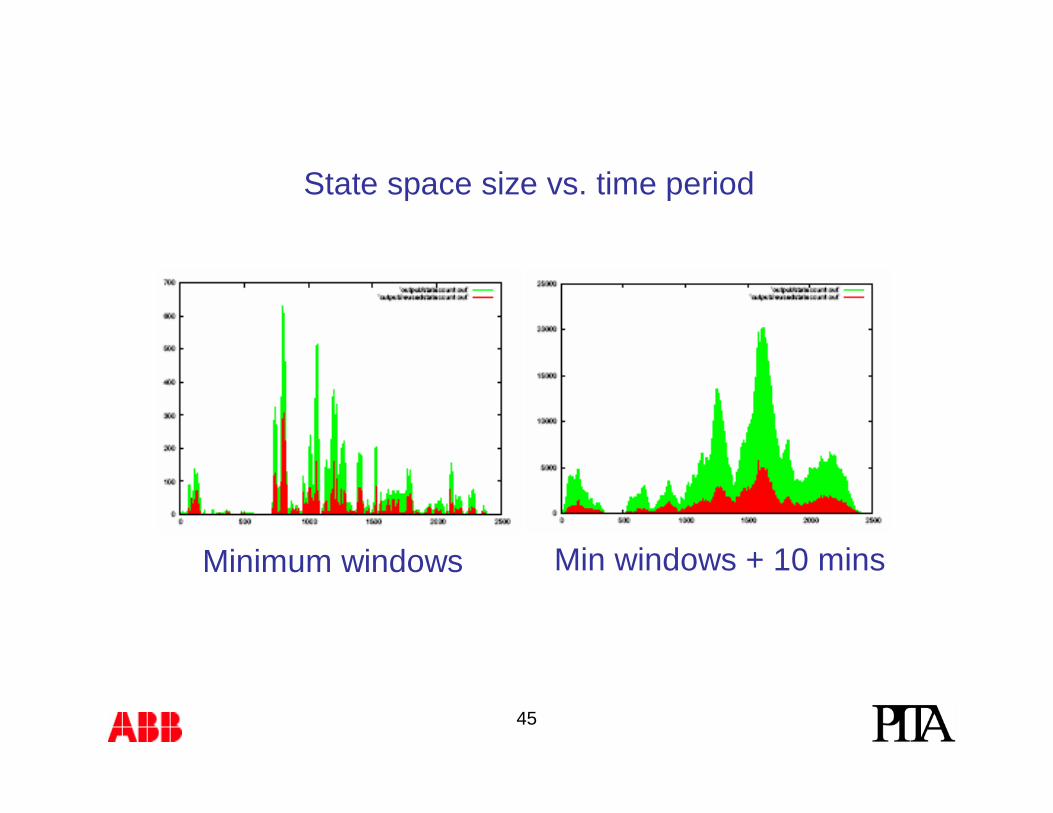
State space size vs. time period
Minimum windows Min windows + 10 mins

46
Computational Results
Problem 2: 258 jobsTime windows specified by client.
?30+30
32*520
18010
Time for one DP (secs)
Minimum time window padding to get feasible
solution (mins)
Jobs
*Multiple DPs solved in some rounds.

47
Solution of 10-job problem
0
100
200
300
400
500
600
0 2 4 6 8 10
’output/solution-time-LEFT.out’’output/solution-time-RIGHT.out’
48
0
2000
4000
6000
8000
10000
12000
14000
0 100 200 300 400 500 600
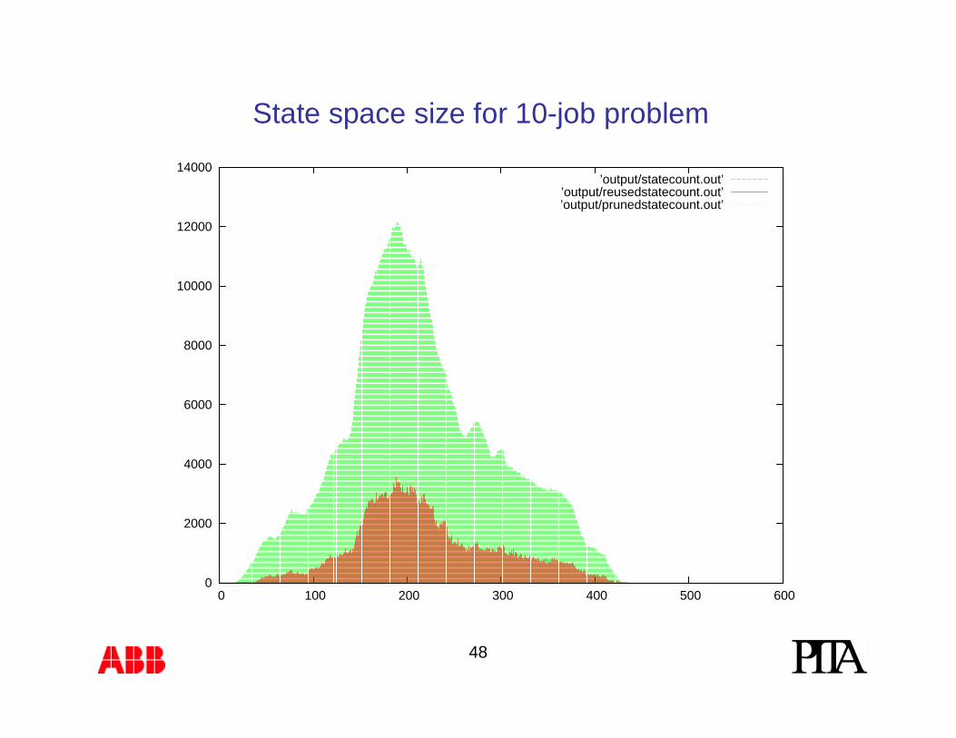
’output/statecount.out’’output/reusedstatecount.out’’output/prunedstatecount.out’
State space size for 10-job problem

49
Computational Results
Problem 2: 258 jobsAdjusted release times.
Same time windows as before.
?30+30
21520
18010
Time for one DP (secs)
Minimum time window padding to get feasible
solution (mins)
Jobs
*Multiple DPs solved in some rounds.

50
Conclusions
• It appears that, in many cases, cranes must lag behind a reasonable production schedule.– Exact algorithm finds no feasible trajectory.
• But it is not enough to spread out the release times.– Certain windows must be very large.– It is hard to predict which ones.
• Due to combinatorial nature of problem.
– So all windows must be stretched.

51
Conclusions
• When all windows are wide, the state space blows up.
• For speed, must solve problem sequentially, a few jobs at a time (e.g., 10).

52
What Next?
• Speed up the DP.– Exploit partial separability of state variables.– Still an exact algorithm, but may not be fast enough.
• Sacrifice exactness for speed.– Use a heuristic dispatching rule.– Rely on same theorem to shape trajectories.– May fail to find feasible solutions, but fast enough for
many assignment/sequencing iterations.

53
Speed Up the DP
• Avoid enumerating states that are identical except for processing times.– Cranes are processing most of the time.– State variables are location and task.– Results in many fewer states.
• Compromise the Markovian property.– When a state has both cranes at stop locations for
their current task…• store costs for different processing times in an array that
persists for several time periods.

54
Speed up the DP
c15c14c13c12c11
c21
c31
c41Compute these costs when a task pair for which both tasks are at their stop locations appears in the state space.
cij = cost-to-go when the left crane has been processing i time units and the right crane has been processing j time units.

55
Speed Up the DP
c21c25c24c23c22
c31c32
c41c42
c11c15c14c13c12Compute these costs in the next period. No need to update existing costs.
Data structure is a 2-dimensional circular queue.
cij = cost-to-go when the left crane has been processing i time units and the right crane has been processing j time units.

56
Speed Up the DP
c32c31c35c34c33
c42c41c43
c12c11c15c14c13
c22c21c25c24c23And similarly in the next period.
cij = cost-to-go when the left crane has been processing i time units and the right crane has been processing j time units.
57
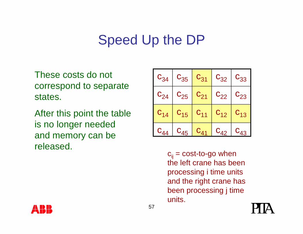
Speed Up the DP
c43c42c41c45c44
c13c12c11c15c14
c23c22c21c25c24
c33c32c31c35c34These costs do not correspond to separate states.
After this point the table is no longer needed and memory can be released.
cij = cost-to-go when the left crane has been processing i time units and the right crane has been processing j time units.

58
Heuristic Dispatching
• Rely on same theorem used by DP to shape the trajectory.– Resulting trajectories are simpler and easier to
implement.
• Use time windows differently.– Time window refers to lapse between start of first task
in a job to completion of last task.• This is impractical in DP because it requires a state variable.
– Production schedule can be revised to reflect resulting job start times.

59
Heuristic Dispatching
• Yield to the other crane only if time still remains to complete remaining tasks in the job.– Allow limited backtracking.– Dispatching rule fails if time runs out.
• Compare with DP on small problems.