Optimal Control of a Drying Process with Avoiding Cracksgrossm/GalGroSchefWen.pdfboundary values,...

Schedae Informaticae Vol. 21 (2012): 81–105

doi: 10.4467/20838476SI.12.006.0816

Optimal Control of a Drying Process with Avoiding Cracks

Alexander Galant2, Christian Grossmann1,Michael Scheffler2, Jorg Wensch1

1Fachrichtung Mathematik, 2Fakultat Maschinenwesen,Technische Universitat Dresden

01062 Dresden, Germany

Abstract. The paper deals with the numerical treatment of the optimal con-

trol of drying of materials which may lead to cracks. The drying process is

controlled by temperature, velocity and humidity of the surrounding air. The

state equations define the humidity and temperature distribution within a sim-

plified wood specimen for given controls. The elasticity equation describes the

internal stresses under humidity and temperature changes. To avoid cracks

these internal stresses have to be limited. The related constraints are treated

by smoothed exact barrier-penalty techniques. The objective functional of the

optimal control problem is of tracking type. Further it contains a quadratic

regularization by an energy term for the control variables (surrounding air)

and barrier-penalty terms.

The necessary optimality conditions of the auxiliary problem form a coupled

system of nonlinear equations in appropriate function spaces. This optimal-

ity system is given by the state equations and the related adjoint equations,

but also by an approximate projection onto the admissible set of controls by

means of barrier-penalty terms. This system is discretized by finite elements

and treated iteratively for given controls. The optimal control itself is per-

formed by quasi-Newton techniques.

2000 AMS subject classifications: 90C25, 90C51, 49K20, 65K10

Keywords: optimal control, penalty barrier methods, control constraints, cou-

pled parabolic system, discretization.

Publikacja objęta jest prawem autorskim. Wszelkie prawa zastrzeżone. Kopiowanie i rozpowszechnianie zabronione. Publikacja przeznaczona jedynie dla klientów indywidualnych. Zakaz rozpowszechniania i udostępniania w serwisach bibliotecznych

82

1. Introduction

The considered models lead to systems of two parabolic partial differential equationsin three spatial variables. This pde system incorporates also phase changes whiche.g. occur in the coupling terms of the system. Diffusion coefficients depend in acomplex way on the state of the system and these dependencies have to be estimatedby experiment. The same holds for the parameters of the evolution equations whichdescribe phase changes. In our model the relevant state variables are temperatureand moisture content of the material. Thus, we obtain an optimal control problemwith a coupled system of time dependent initial-boundary value problems as stateequations (cf. [24]). The numerical solution of the direct problem requires discretiza-tion in time and space. Time discretization is done by the implicit Euler method.The resulting elliptic system is discretized by the conforming Finite Element methodon a triangular grid with linear elements. The drying process is controlled via theboundary values, namely temperature, moisture and velocity of the surrounding air.The objective of the process is to reduce the moisture of wood up to a prescribeddegree under minimal energy. In order to avoid cracks (see [20]), restrictions oninternal tensions are treated by a smoothed exact penalty method (see [11]). Anefficient evaluation of gradients via the adjoint system for the time-discretized modelis applied.

As a particular example we consider the industrial wood drying performed indrying chambers. On the one hand, a simplified form of this technological processfits directly into the discussed general approach and on the other hand some func-tional dependencies from wood drying are used to illustrate the model. The wooddrying process is controlled by various functions like outer temperature, humidityand velocity of the surrounding air. The aim of the present paper is to report on anoptimization approach to this task by gradient based methods. In the literature thereis a rather wide variety of models for wood drying, see e.g. [4, 5, 12, 14, 19, 25, 16].

Models based on physical principles use a multiple component approach. Thereare three phases of water, namely liquid water, vapor and bound water. Phasechanges occur due to pressure and temperature variations. Fluid transport is causedmainly by diffusion. In addition, advection may be caused by pressure gradients.Vapor is modeled as a component of a mixture of air and vapor underlying advectionand diffusion. Advection and diffusion of vapor is computed as multi component flowof the air-vapor mixture driven by pressure and concentration gradients.

The drying process is controlled via the boundary values, namely temperature,moisture and velocity of the surrounding air. The objective of the process is to reducethe moisture of wood up to a prescribed degree under minimal energy. In order toavoid cracks (see [20]), restrictions on internal tensions are included into the problemby a smoothed exact penalty method (see [11]). For results on optimal control ofpartial differential equations, we refer e.g. to [3, 11, 13, 24]. Having gradient basedoptimization as optimization technique in mind the efficient evaluation of gradientsvia adjoint systems is studied in Section 3. In particular, the adjoint system for thetime-discretized model is derived.

The paper is structured as follows. In Section 2 we describe a rather abstract


83

formulation of the underlying model for the direct problem as a system of evolutionequations. Further the discretization by finite elements is briefly described and thegradient evaluation via adjoints is outlined. A simplified model of wood dryingis derived in Section 3. In Section 4 we report on numerical results, both, thedirect simulation with discretization techniques as well as the solution of the optimalcontrol problem by gradient-based techniques of Quasi-Newton type. Finally a shortsummary in Section 5 concludes the paper.

2. The abstract control problem

2.1. The control problem

In this section we discuss a class of boundary optimal control problems with asystem of quasi-linear parabolic partial differential equations as state equations andpointwise control and nonlinear state constraints. Many application problems canbe embedded into this general framework.

We consider the nonlinear control problem

J(y, u) :=n∑i=1

µi2

∫Ω

(yi(·, T )− yd,i)2 dΩ +m∑j=1

αj2

∫ T

0

(uj − ud,j)2 dt −→ min (1a)

subject to

yt + A (y)y = 0, in Ω× (0, T ]B(y)y = g(y, u), on Γ× (0, T ]y(·, 0) = y0 on Ω

(1b)

ua ≤ u ≤ ubσa ≤ σ(y) ≤ σb.

(1c)

In this setting Ω ⊂ RN , N ∈ N denotes a bounded domain which has a piecewise C1,1

boundary Γ and T is a fixed time horizon. For a given initial value y0 we will seek theoptimal control u : [0, T ] → Rm with associated optimal state y : Ω × [0, T ] → Rn.The objective functional J represents a classic form, in which the first term is oftracking type that minimizes the difference between the state values y(·, T ) at theend time T and the target values yd. The second term is a regularization, where uddenotes some energy minimal control. The parameters µi and αj are scaling andregularization parameters, respectively. We consider bounds ua, ub ∈ Rm, ua ≤ uband σa, σb ∈ R, σa ≤ σb. The operator A (y) is (uniformly) elliptic of the type

A (y)z = −N∑j,k

∂j(ajk(y)∂kz) (2)


84

and B(y) denotes the related boundary operator of Neumann type. Moreover, thenonlinear functions σ : Rn → R, g : Rn × Rm → Rn and ajk : Rn → Rn×n, j, k =1, . . . , N are given.

In the sequel we apply the following notation: By (·, ·) and ‖ · ‖ we denote theinner product in L2(Ω) and the related norm, respectively. Further, we introducefollowing spaces with usual product topologies V := H1(Ω)n, H := L2(Ω)n andU := L∞(0, T )m. With < ·, · > we denote duality pairing between V its dual spaceV∗.

Let us start the discussion with the state equations (1). The abstract problem(1b) can be described by a system of variational equations. With the bilinear form

a(y; ·, ·) : V ×V→ R defined by a(y; z, v) :=N∑

j,k=1

∫Ω

ajk(y)∂kz · ∂jv dΩ

and the linear form(g(y, u), ·)Γ : V→ R

defined by

(g(y, u), v)Γ :=

∫Γ

g(y, u) · v dΓ for all (y, u) ∈ V ×U,

we obtain the following weak formulation:

〈yt, v〉+ a(y; y, v) = (g(y, u), v)Γ ∀ v ∈ V t ∈ (0, T ],y(0) = y0.

(3)

For our further analysis we introduce the set of admissible controls for (1) by

Uad := u ∈ U : ua ≤ u(·) ≤ ub a.e. in (0, T ).

Theorem 1. Under the assumptions:

A1: Ω be a bounded region in RN with ∂Ω ∈ C∞;

A2: The coefficients g, ajk,∀j, k = 1, . . . , N are C∞ for all y ∈ Ω and u ∈ Uad;

A3: (Ellipticity of A ): for each y ∈ Rn and ξ ∈ Rn with |ξ| = 1, all the eigenvaluesof the n× n-matrix ajk(y)ξjξk have a positive real part;

the following statements are true:

(a) (Existence and Uniqueness): For any (y0, u) ∈ H × U the parabolic initial-boundary value problem (1b) possesses a unique (weak) solution y ∈ W (0, T ),where the space W (0, T ) is given by W (0, T ) := y ∈ L2(0, T,V) : yt ∈L2(0, T,V∗) .

(b) (Differentiability): The solution y(t) depends in the topology of W (0, T ) smoo-thly upon y0 and u. Particularly, for each w ∈ U the function

p(·) = ∂uy(·, y0, u)w

is equal to the solution of the initial-boundary value problem, which is obtainedby differentiating the original problem (1b) formally with respect to u in thedirectional w.


85

For the proof we refer to [1] Theorem 7.1, 7.3 and 11.1 as well as to [27] Theorem31.C.

Hence, by Theorem 1, the parabolic initial-boundary value problem governing(1) admits for each u ∈ Uad a unique weak solution y ∈ W (0, T ). This allows usto introduce the control-to-state operator S : Uad → W (0, T ) : u 7→ y. With thissetting we will reformulate the general problem to the reduced form:

f(u) := J(S(u), u) −→ min! (4a)

subject to

u ∈ Uad, σa ≤ σ(S(u)) ≤ σb. (4b)

For the treatment of the state constraint (4b) we apply the penalization technique,based on smoothed exact penalty function

η(a− ξ +

√(a− ξ)2 + s2

)with the parameters η, s ∈ R which for s→ 0+ approximates the well known exactpenalty

2 ηmax0, a− ξ

to treat the constraint a − ξ ≤ 0. In the considered case of (4b) this leads up to aconstant to

Pη(ξ; a, b, s) := η(√

(ξ − a)2 + s2 +√

(ξ − b)2 + s2)

≈ η (|ξ − a|+ |ξ − b|),(5)

where s > 0 is a smoothing parameter that tends in the limit to 0, and η > 0is a fixed parameter that is sufficiently large to ensure the exactness of underlinedpenalty η (|ξ−a|+|ξ−b|) (cf. [10]). We, hence, consider a purely control-constrainedand smooth problem

fη(u) := f(u) +

T∫0

∫Ω

Pη(σ(S(u));σa, σb, s) dΩ dt −→ minu∈Uad

, (6)

where the state constraints have been handled by penalization (5). For the conver-gence of this barrier-penalty method in the finite dimensional case we refer to [10].We meet this case later since the problem will be discretized by finite elements.

We remark that in the case of the infinite problem the constraints upon σ(y)have to be considered pointwise to guarantee the existence of optimal Lagrangemultipliers, which in this case are Borel measures.

Under certain additional conditions, e.g. linearity of the control in the stateequation, one can show the existence of at least one globally optimal control u∗ withassociated optimal state y∗ for (6), provided the set of admissible controls Uad is notempty. The associated first-order necessary optimality conditions can be determinedby a standard computation.


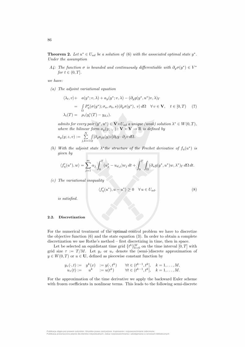
86

Theorem 2. Let u∗ ∈ Uad be a solution of (6) with the associated optimal state y∗.Under the assumption

A4: The function σ is bounded and continuously differentiable with ∂yσ(y∗) ∈ V ∗for t ∈ (0, T ].

we have:

(a) The adjoint variational equation

〈λt, v〉+ a(y∗; v, λ) + ay(y∗; v, λ)− (∂yg(y∗, u∗)v, λ)Γ

=∫Ω

P ′η(σ(y∗);σa, σb, s)〈∂yσ(y∗), v〉 dΩ ∀ v ∈ V, t ∈ [0, T )

λi(T ) = µi(y∗i (T )− yd,i).

(7)

admits for every pair (y∗, u∗) ∈ V×Uad a unique (weak) solution λ∗ ∈W (0, T ),where the bilinear form ay(y; ·, ·) : V ×V→ R is defined by

ay(y; z, v) :=N∑

j,k=1

∫Ω

[∂yajk(y)z]∂ky · ∂jv dΩ.

(b) With the adjoint state λ∗the structure of the Frechet derivative of fη(u∗) isgiven by

〈f ′η(u∗), w〉 =m∑j=1

αj

∫ T

0

(u∗j − ud,j)wj dt+

∫ T

0

∫Ω

(∂ug(y∗, u∗)w, λ∗)Γ dΩ dt.

(c) The variational inequality

〈f ′η(u∗), u− u∗〉 ≥ 0 ∀u ∈ Uad. (8)

is satisfied.

2.2. Discretization

For the numerical treatment of the optimal control problem we have to discretizethe objective function (6) and the state equation (3). In order to obtain a completediscretization we use Rothe’s method – first discretizing in time, then in space.

Let be selected an equidistant time grid tkMk=0 on the time interval [0, T ] withgrid size τ := T/M . Let yτ or uτ denote the (semi-)discrete approximation ofy ∈W (0, T ) or u ∈ U, defined as piecewise constant function by

yτ (·, t) := yk(x) := y(·, tk) ∀t ∈ (tk−1, tk], k = 1, . . . ,M,uτ (t) := uk := u(tk) ∀t ∈ (tk−1, tk], k = 1, . . . ,M.

For the approximation of the time derivative we apply the backward Euler schemewith frozen coefficients in nonlinear terms. This leads to the following semi-discrete


87

optimal control problem:

Jτη (yτ , uτ ) :=∑ni=1

µi2 ‖y

Mi − yd,i‖2 + τ

∑mj=1

αj2

∑Mk=1(ukj − ud,j)2

+τ∑Mk=1

∫ΩPη(σ(yk);σa, σb, s) dΩ −→ min

(9a)

subject to constraints given by the semi-implicit discretization

1

τ(yk − yk−1, v) + a(yk−1; yk, v) = (g(yk−1, uk), v)Γ, ∀ v ∈ V, k = 1, . . . ,M (9b)

uτ ∈ Uτad, (9c)

where y0 is given by the initial conditions. For the discretization in space we in-troduce an inner convergent approximation of space V set by the triples family(Vh, ph, rh)h∈H , whereVh – space of linear conform finite elements,ph – prolongation operator from Vh to V given by identity,rh – restriction operator from V to Vh defined as L2-projection.Further, we define yτ,h as a finite element approximation of yτ by

yτ,h(·, t) := ykh(·) := rhyτ (·, t) ∀t ∈ [tk−1, tk], k = 1, . . . ,M.

The full discretization of the control problem is finally obtained from (9) by the useof finite-dimensional space Vh instead of the space V:

Jτ,hη (yτ,h, uτ ) :=∑ni=1

µi2 ‖y

Mh,i − rhyd,i‖2 + τ

∑mj=1

αj2

∑Mk=1(ukj − ud,j)2

+τ∑Mk=1

∫ΩPη(σ(ykh);σa, σb, s) dΩ −→ min

(10a)

subject to

1τ (ykh − y

k−1h , vh) + a(yk−1

h ; ykh, vh) = (g(yk−1h , uk), vh)Γ ∀ vh ∈ Vh, k = 1, . . . ,M,

y0h = rhy

0,

(10b)

uτ ∈ Uτad. (10c)

Owing to linearity and to finite-dimensionality, the discrete state equation (10b)admits, obviously, for every pair (y0

h, uτ ) ∈ Vh ×Uτ a unique solution yτ,h. Thisallows us to introduce the analogue of control-to-state operator in discrete caseSτ,h : Uτad → L2(0, T,Vh) : uτ 7→ yτ,h and to rewrite (10) in condensed form

fτ,hη := Jτ,hη (Sτ,h(uτ ), uτ ) −→ minuτ∈Uτad

. (11)

The control problem (11) has at least one solution, since Uτad is not empty and theproblem is penalized. Again, as in the continuous case, the non-convexity of theproblem may cause multiple local optima.


88

2.3. Gradient computation by adjoint techniques

We follow here the ’first discretize, then optimize’ strategy. The finite-dimensionalproblem (10) is a large-scale nonlinear minimization problem with constraints. Usingthe constraints to eliminate y we arrive at (11) we obtain a large-scale nonlinearminimization problem where the only constraints are the box constraints on thecontrol. Techniques to compute minimizers of such problems involve the evaluationof the gradient of the objective function.

Here, we derive a discrete adjoint equation by applying the standard Lagrangianprinciple, where the discretized state equation is eliminated by Lagrangian multipli-ers.

To simplify the notation we use the discrete variables y, u, λ without subscriptsτ, h in the following part.

We couple the constraint – M steps of the backward Euler method – by La-grangian multipliers to Jτ,hη (y, u). The result is abbreviated by Jλ. The Lagrangian

multipliers λk ∈ Vh are determined such that the variation of Jλ does not dependon variations of y. This is accomplished by applying the discrete analog of partialintegration.

7Jλ = Jτ,hη (y, u) + Cλ with

Cλ =M∑k=1

(〈λk, yk − yk−1〉+ τa(yk−1; yk, λk)− τ(g(yk−1, uk), λk)Γ

)=

M−1∑k=0

〈λk − λk+1, yk〉 − 〈λ0, y0〉+ 〈λM , yM 〉

+τM∑k=1

(a(yk−1;λk, yk)− (g(yk−1, uk), λk)Γ

).

The first variation of Jτ,hη (y, u) is given by

δJτ,hη (y, u) =n∑i=1

µi〈yMi − yd,i, δyMi 〉

+ τM∑k=1

∫Ω

P ′η(σ(yk)) 〈∂ykσ(yk), δyk〉 dΩ + τ

M∑k=1

m∑j=1

αj(ukj − ud,j)δukj

whereas the variation of the coupled constraint evaluates to

δCλ =M−1∑k=1

〈λk − λk+1, δyk〉+ 〈λM , δyM 〉

+ τM∑k=1

a(yk−1;λk, δyk) + τM−1∑k=1

⟨∂yka(yk;λk+1, yk+1), δyk

⟩− τ

M−1∑k=1

⟨∂yk(g(yk, uk+1), λk+1)Γ, δy

k⟩− τ

M∑k=1

∂uk(g(yk−1, uk), λk)Γ δuk.


89

Putting all together, for the variation of Jλ finally we obtain

δfτ,hη =δJλ = τM∑k=1

m∑j=1

(αj(u

kj − ud,j)− ∂ukj (g(yk, uk), λk)Γ

)δukj

whenever λ the terminal condition at t = tM

1

τ

n∑i=1

〈λMi + µi(yMi − yd,i), vi〉+ a(yM−1;λM , v) =

∫Ω

P ′η(σ(yM )) 〈∂yMσ(yM ), v〉 dΩ

∀v ∈ Vh and a discrete recursion

1τ 〈λ

k − λk+1, v〉+ a(yk−1;λk, v) = −⟨∂yka(yk;λk+1, yk+1), v

⟩+⟨∂yk(g(yk, uk+1), λk+1)Γ, v

⟩−∫Ω

P ′η(σ(yk)) 〈∂ykσ(yk), v〉 dΩ ∀v ∈ Vh.

This allows to evaluate the gradient efficiently by a discrete linear parabolic problem.

3. Application to a model for wood drying

As already mentioned, wood drying forms a complex physical model that involvesheat and humidity transfer inside the material as well as exchange processes with thesurrounding media at the surface of the wood. In the sequel we describe a simplifiedmodel which is later used in practical applications of wood drying.

The state variables of our process are moisture content X and temperature ϑinside the wood specimen, i.e. y = (X,ϑ). Thereby, X is given by X = (mw −md)/(md) where mw denotes the mass of the wet and md the mass of the ovendry material. As control variables u = (vL, YL, ϑL) we have the velocity, absolutehumidity and temperature of the surrounding air, respectively. As reference controlsud = (vL,d, YL,d, ϑL,d) we applied vL,d ≡ 0 m/s, YL,d ≡ 0.01038649 kg/m

3, ϑL,d ≡

20oC (YL,d corresponds to relative humidity ϕL = 60% and to temperature ϑL =20oC). These reference controls serve in fact regularizing terms in the objectivefunction. Their values correspond to typical values from practical experience.

The aim of wood drying is to achieve a given target value Xd of the moisturecontent X inside the wood specimen. Thus, we have the objective function (1a)with (y;u) = (X,ϑ; vL, YL, ϑL), µ = (1, 0) and problem dependent regularizationparameters α = (α1, α2, α3).

The stresses σ in (1c), (6) are described in Subsection 3.2. below. The remainingparameters (lower, upper control and stress bounds, target humidity, etc.) will beset in Section 4. on the numerical experiments.


90

3.1. Heat and mass transfer

Our approach bases upon some heat-and-mass transport model by Vogel [25], wheresome minor modifications were done.

In the transport model the following simplifying assumptions are made:

1. We ignore the fiber structure, i.e. an isotropic homogeneous hydroscopic ma-terial is assumed.

2. For heat and mass transfer through the boundary surface we consider heatconduction and radiation, but condensation by sprayed vapor from outside isnot considered.

3. The enthalpy for the phase change of water is restricted to the boundary ofthe wood specimen.

4. The total moisture distribution is considered as a uniform diffusion process.

Such a minimal model on the one hand is able to explain the main effects of a physicalprocess while on the other hand it limits the computational effort for its solution.The model was justified by experiments for different application cases such as wooddrying and humidity diffusion between different climates [20, 2]. This can be seene.g. in Fig. 1 from [2] which provides a comparison of a fully-coupled simulationbased on the code Delphin 4 [6] with our minimal model. The maximal differencesare ≈ 1%.

Figure 1.: Comparison of calculation of a diffusion process in wood based materials with thefully-coupled Code Delphin 4 (left) and the minimal model (right)

Let Ω ⊂ Rn with n ∈ 2, 3 denote some bounded convex domain with a piecewisesmooth boundary Γ = ∂Ω and let T > 0 denote some fixed terminal time. Theinternal stress depends upon the volume changes. These are inflicted by changesof the moisture content field X. Further, the local changes in the moisture contentdepend upon the temperature field ϑ. Under the made assumptions this can bedescribed by a system of nonlinear parabolic differential equations

Xt = ∇(D(X,ϑ)∇X) in Ω× (0, T ],

ϑt = 1ρdtcp

∇(λ(X,ϑ)∇ϑ) in Ω× (0, T ](12)


91

with initial conditions

X(·, 0) = X0, ϑ(·, 0) = ϑ0 on Ω. (13)

Here D and λ are the coefficients of diffusion and heat conduction, respectively.These coefficients depend upon the moisture content X and the temperature ϑ. Theconstant parameters ρdt and cp denote the density of the bone-dry wood and thespecific heat coefficient, respectively. The heat conduction coefficient λ = λ(X,ϑ) iscalculated as follows: With some chosen parameter X12 (in our calculations X12 =0.12) and with with ρdt, cp we define

ρ12 := ρdt1 +X12

1 + 0.84ρdt

1000X12

,

λ0 := 0.195 · 10−3ρ12 + 0.0256,

λ(X,ϑ) := λ0 (0.85 + 1.25X)(

1− (1.1− 0.98 · 103ρdt)(0.27 + ϑ100

)).

(14)

We model the boundary conditions for the humidity such that the amount of watertransported by convection is proportional to the gradient of the inner moisture profileat the boundary. This yields

β(vL)(YL − Y (X,ϑ)) = ρdtD(X,ϑ)∂X

∂νon ∂Ω× (0, T ]. (15)

For the modeling of vaporization coefficient β the Lewis’ analogy

β(vL) =α(vL)

cpL

is used, where α denotes the heat-transfer coefficient, vL is the given velocity of the

surrounding air, and cpL = 1, 0054

[kJ

kgK

]the constant air specific heat. Further, Y

describes the equilibrium moisture content and depends upon the moisture contentX at the surface of the wood as well as upon the temperature ϑ. The control variableYL denotes a given moisture profile of the surrounding air.

Now, it remains only to derive the boundary condition for the temperature. Theinfluence of the convective heat flow that controls the drying process is split into itseffect upon the material warming and upon the evaporation of water, i.e.

α(vL)(ϑL − ϑ) = λ(X,ϑ)∂ϑ

∂ν+ β(vL)hv(X,ϑ)(Y (X,ϑ)− YL) on ∂Ω× (0, T ], (16)

where α denotes the heat-transfer coefficient, hv the additively combined bondingand evaporation enthalpy, and ϑL the given temperature of the surrounding air. Theheat-transfer coefficient due to Krecetov [18] is given by

α = α(vL) = 6.2 + 4.2vL,

and the enthalpy according to Kayihan–Stanish [16] by

hv(X,ϑ) =

267(374− ϑ)0.38(1 + 0.4(1− X

0.3)), for X < 0.3

267(374− ϑ)0.38, otherwise.


92

For modeling the equilibrium moisture content Y depending on air humidity calledsorption hysteresis we apply Krecetov’s approach [18]. In this model the moistureX at the boundary of the wood relates to the relative humidity ϕ and to the tem-perature ϑ according to

X(ϕ, ϑ) =

0.36100

(13.9−B(ϑ)) + 0.72100

(29.5−B(ϑ))ϕ, ∀ϕ ∈ [0, 0.5]

0.512(21.7−B(ϑ))100 (1.21− ϕ)

, ∀ϕ ∈ (0.5, 1](17)

where B(ϑ) = ((ϑ+ 273.2)/100)2. For simplicity we assume that at fiber saturation(ϕ = 1) independently within the considered temperature range holds XFSP = 0.3and that the moisture content X at 50% relative humidity (ϕ = 0.5) independentlyof the temperature has the value X1/2 = 0.08. Now, we obtain the required inversemapping

ϕ(X,ϑ) =

X − 0.36100

(13.9−B(ϑ))

0.72100

(29.5−B(ϑ)), X ≤ X1/2

1.21−0.512100

(21.7−B(ϑ))

X, X1/2 < X < XFSP

1.21−0.512100

(21.7−B(ϑ))

XFSP, X ≥ XFSP .

(18)

The relative humidity ϕ relates to the absolute humidity Y by

Y (X,ϑ) = δ · ϕ(X,ϑ)E(ϑ), (19)

where δ = 0.622/p at the normal pressure p = 1000[hPa] is a constant and

E(ϑ) = 6.1078 · exp

(17.08085 · ϑ234.175 + ϑ

)(20)

represents the saturation pressure.The approach of Dushman–Lafferty [7] for the diffusion coefficient of water vapor

DV below the fiber saturation point yields

DV (X,ϑ) = 0.22 · 10−4 p

R

ρw + ρzwX

ρwρzw

(ϑ+ 273

273

)1.751

ϑ

∂ϕ

∂X(X,ϑ), (21)

where p is the normal pressure, R the universal gas constant, ρw denotes the densityof water and ρzw the density of the cell wall. For ρw and ρzw we put the constant

values 1000 [kg/m3] and 1510 [kg/m

3], respectively.

∂ϕ∂X

(X,ϑ) in equation (21)

means the slope of the absorption isotherms that can be calculated via the formula(18).

The transport of bound water below the fiber saturation point we follows theArrhenius’ law

DB(X,T ) = 7 · 10−6 · exp (− E0(X)

R(ϑ+ 273)),


93

with the universal gas constant R and the activation energy

E0(X) = 3.86 · 104 − 2.94 · 104X.

Siaus’s analogy [21] leads to the following transport model

D(X,ϑ) =1

1− ap(X,ϑ)2

DB(X,ϑ)DV (X,ϑ)

DB(X,ϑ) + (1− ap(X,ϑ))DV (X,ϑ), X ≤ XFSP (22)

where ap denotes the edge length of the cross-section of square pore, that can becalculated from the porosity of the solid body va

ap(X,ϑ) =√va ≈

√1− ρ(X)

ρw

0.667 +X

1 +X.

The density of the humid wood under the fiber saturation point is given by

ρ(X) = ρdt1 +X

1 + 0.84Xρdt

1000

.

Above the fiber saturation point, i.e. for X > XFSP . we apply Koponen’s [17]concept, that uses the diffusion coefficient in fiber saturation point as initial value

D(X,ϑ) = D(XFSP , ϑ)(1− 0.8845 · k(X) + 0.2525 · k(X)2)

with k(X) = X −XFSPρwρdt

(1− ρdtρzw

)−XFSP

. (23)

The described model can be embedded easily into the abstract mathematicalmodel of the state equation (1b).

3.2. Elastic model for stress evaluation

Our elastic model follows Siimes’s [22] model with the simplifying assumptions:

1. The (rectangular) shape of a specimen crosscut remains unchanged duringdrying.

2. We approximate the total stress by a coordinate splitting approach.

3. The resulting external forces in the x and in the y-direction vanish.

We have to provide a model for the evaluation of the internal stresses σ. Thechanges in length are denoted by ∆lx and ∆ly and the lengths of specimen in x-and y-direction are defined by lx and ly, respectively. The approach is described forthe x-direction below, the results for the y-direction are obtained in a similar way.


94

Moisture content X induces a relative change of the volume as well as a changeof the module of elasticity. The volumetric change induces a free strain εxfree(x, y).Neglecting shear effects, we have an averaged free length change

∆lxfree(y) =

∫ lx

0

εxfree(x, y)dx.

By Assumption 1, we observe a constant length change

∆lxobs =

∫ lx

0

εxobs(x)dx

that is independent of y. The difference of both strains yields the effective strain

εxeff (x, y) =εfree(x, y)− εxobs(x). (24)

Now, the stresses follow Hooke’s law,

σx(x, y) = E(x, y)εxeff (x, y). (25)

Due to Assumption 3 we have ∫ ly

0

σx(x, y) dy = 0.

Hence,

εxobs(x) =

ly∫0

E(x, y)εfree(x, y) dy

ly∫0

E(x, y) dy

.

Combining the stresses in the x- and y-directions, we obtain the total stress

σ(x, y) = |σx(x, y)|+ |σy(x, y)|. (26)

Finally, we have to supply models for the elasticity module E and the free strainεfree. One possibility is due to Welling [26]

E(x, y) = E(X(x, y)) =

E(X = 0.08), X < 0.08EB(ρdt)(0.904− 4.37(X − 0.12)), 0.08 ≤ X ≤ 0.18E(X = 0.18), X > 0.18

where EB(ρdt) = 40 + 2.12 · 10−3ρ2dt. Further, we apply the Ansatz

εfree(x, y) = εfree(X(x, y)) =

α(X = 0.3)− α(X)1− α(X = 0.3)

, X < 0.3

0, otherwise

with α(X) =0.84 · 10−3ρdtX

1.360 + 4.394 · 10−4ρdt − 5.179 · 10−8ρ2dt

.


95

4. Numerical experiments

4.1. Simulation of the direct problem

Before we turn to optimal control we have to validate the used simplified modeldescribed in the previous sections. For this purpose among other test problems weselected some practical experiment reported in [12]. These results are comparedwith those obtained by our computer simulation.

The state equations are discretized by piecewise linear C0-element techniqueover triangular grids. The underlying finite element geometry was generated by theprogram package FEMLAB (see http://www.comsol.com/).

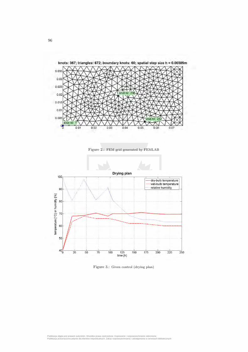
As common in wood engineering, we represent the control u = (vL, YL, ϑL), i.e.the air velocity, the absolute air humidity and air temperature in the drying chamberin form of a drying plan. Dry-bulb and wet-bulb temperatures of psychrometer aredepicted on the drying plan. The required absolute and relative humidity can becalculated from these data. In our experiments the air velocity was considered asconstant.

In addition to the simulated and measured mean humidity, in both examples wedescribe the moisture development in three reference knots. These knots are chosenin such that they represent typical areas of the specimen. This is achieved by point1 – at the boundary, point 2 – in the center of the domain and point 3 – inside, butvery close to the boundary.

Example 1

In Fig. 4 we illustrate the effect of oscillating relative humidity (compare dryingplan, Fig. 3) in form of a stepwise course of the mean humidity of wood. Again, theexperimental data are in accordance with the simulation results.

Table 1.: Data for Example 1

Air velocity 1ms Oven dryness 700

kgm3

Sample size 38×77 mm Drying time 250hInitial humidity 31% Initial temperature 40CTime step size 600s Spatial step size 3.85 mm


96

Figure 2.: FEM grid generated by FEMLAB

Figure 3.: Given control (drying plan)


97

Figure 4.: Humidity change

Table 2.: Deviation of the simulation from the measurement

Error maximum mean root-mean-square[kgkg

]0, 018 0, 009 0, 011

Figure 5.: Humidity distribution after 125h, 167h and 250h

The obtained results for the simulation of the direct problem are qualitatively (seeFig. 4) as well as also quantitatively (compare Tab. 2) in very good agreement withthe experimental data. This provides a justification for the use of the simplifiedpresented above for the wanted optimal control.


98

4.2. Optimal control experiments

While in the previous subsection we reported on some results for the direct problem,i.e. some problem with given controls (drying plans) here we consider the generationof drying plans by optimization techniques. The data of the reported examples aregiven in the Tab. 3 below. All numerical experiments are executed for the case ofzero-regularization (i.e. α = (α1, α2, α3) = (0, 0, 0) in (1a)). This is possible becausethe penalty already provides a regularizing effect. Furthermore, the control is alsopenalized, i.e. the term

3∑i=1

∫ T

0

Pη(ui(t), ua,i, ub,i, s) dt

is added to the objective function (compare eq. (6)). That leads to an unconstrainedoptimization problem. As optimization methods gradient based techniques havebeen applied where the gradients are efficiently evaluated via adjoint equations.

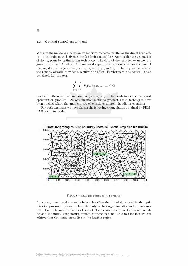
For both examples we have chosen the following triangulation obtained by FEM-LAB computer code.

Figure 6.: FEM grid generated by FEMLAB

As already mentioned the table below describes the initial data used in the opti-mization process. Both examples differ only in the target humidity and in the stressrestriction. The initial values for the control are chosen such that the initial humid-ity and the initial temperature remain constant in time. Due to that fact we canachieve that the initial stress lies in the feasible region.


99

Table 3.: Initial optimization data

Example 2 Example 3Oven dryness 700 kg/m3 700kg/m3

Sample size 50×100 mm 50×100 mmInitial humidity 22% 22%Initial temperature 8 C 8 CTime step size 600 s 600 sSpatial step size 5 mm 5 mmDrying time 24 h 24 hTarget humidity 21% 16%Stress bounds ±10 mPa ±25 mPaLower control bounds 0 m/s, 5%, 5 C 0 m/s, 5%, 5 CUpper control bounds 10 m/s, 95%, 85 C 10 m/s, 95%, 85 C

For the optimization a restart version of Broyden’s method has been applied withthe identity matrix as initial approximation of the Jacobian. After 100 iteration stepsthe restart procedure, i.e. the iteration matrix is again set to the identity. Further,at restart the penalty parameter is reduced by a fixed multiplier.

Similarly to the direct simulation we choose three reference knots (see Fig. 6) toobserve the state of humidity and elastic stress at these points.

Figure 7.: Computed velocity after 4 iterations Example 2


100

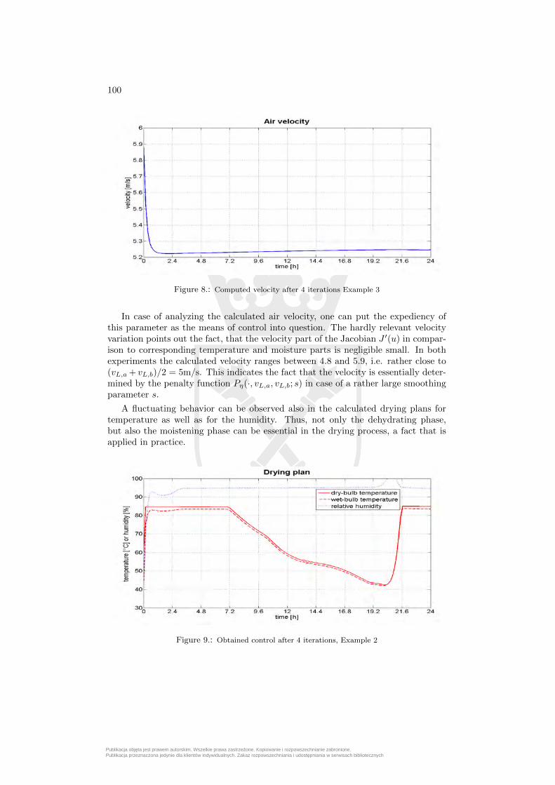
Figure 8.: Computed velocity after 4 iterations Example 3

In case of analyzing the calculated air velocity, one can put the expediency ofthis parameter as the means of control into question. The hardly relevant velocityvariation points out the fact, that the velocity part of the Jacobian J ′(u) in compar-ison to corresponding temperature and moisture parts is negligible small. In bothexperiments the calculated velocity ranges between 4.8 and 5.9, i.e. rather close to(vL,a + vL,b)/2 = 5m/s. This indicates the fact that the velocity is essentially deter-mined by the penalty function Pη(·, vL,a, vL,b; s) in case of a rather large smoothingparameter s.

A fluctuating behavior can be observed also in the calculated drying plans fortemperature as well as for the humidity. Thus, not only the dehydrating phase,but also the moistening phase can be essential in the drying process, a fact that isapplied in practice.

Figure 9.: Obtained control after 4 iterations, Example 2


101

Figure 10.: Obtained control after 4 iterations, Example 3

The qualitative behavior of the optimal control variables differs for the two dif-ferent experiments. In Example 3 a mean target humidity of 16% (a loss of 6%moisture) after 24 hours is required. Most wood materials even under the relativelyweak stress bounds ±25 mPa (see Tab. 3) can lose only a small part of moisture.This leads us to the straightforward solution strategy, in which almost everywherethe highest admissible air temperature and the smallest admissible air humidity arechosen such that the stress bounds are active at the boundary.

In Example 2 a moderate moisture loss of only 1% is required. This leads us toa solution (see Fig. 10, on the left) where the inequality restrictions for the controlsare active. The solution has the property that the mean target humidity of 21% isalmost achieved. The stress is widely within the given bounds. At the same time(see Fig. 12) the boundary humidity exceeds for a short term the initial humidity(moistening). Interesting is also that the stress at the end of the drying sink is nearlyby zero again (see Fig. 14, on the left).

Figure 11.: Humidity in reference knots, Example 2


102

Figure 12.: Humidity in reference knots, Example 3

Figure 13.: Stress in reference knots, Example 2

Figure 14.: Stress in reference knots, Example 3

Some quantitative results of both experiments are summarized in Tab. 4. One


103

can see that the required mean target humidity is almost achieved. The stress andcontrol bounds are both broken.

Table 4.: Some quantitative results

Example 2 Example 3Mean humidity (T = 24h) 21.22% 16.49%Min stress −5.0 mPa −11.7 mPaMax stress 11.9 mPa 25.3 mPaMin control values 4.8 m/s, 40.0%, 42.4 C 5.2 m/s, 30.0%, 50.0 CMax control values 5.9 m/s, 100.0%, 85.0 C 5.9 m/s, 77.3%, 93.3 C

Bounds breaking can be reduced through decreasing of corresponding penaltyparameters. The problem of the control bounds breaking can be avoided thanks toapplication of the methods for the constrained optimization, e.g. [10]. Moreover,if the regularization is used (that means α 6= 0, compare Eq. (1a)), it will beautomatically provided, that the control lie near the energy minimal control (costminimization) and so are feasible.

It must be mentioned that the stress bounds in all our experiments are brokenonly during the short time at the beginning of drying. This result can still beacceptable for the wood drying, since at the beginning, where the moist materialhas sufficient viscosity, the stress bounds are less critical than during the rest timeof drying.

5. References

[1] Amann H.; Dynamic theory of quasilinear parabolic equations. I. Abstract evolutionequations, Nonlinear Analysis: Theory, Methods and Applications 12, 1988, pp.895–919.

[2] Branke D., Kroppelin U., Scheffler M., Thielsch K.; Simulationsmodell fr Holzw-erkstoffplatten unter Differenzklimabeanspruchung, Holztechnologie 48 (1), 2007,pp. 25–29.

[3] Casas E., Mateos M.; Uniform convergence of the FEM applications to state con-strained control problems, Comput. Appl. Math. 21, 2002, pp. 67–100.

[4] Ciegis R., Starikovius V.; Mathematical modelling of wood drying process, Math.Model. Anal. 7(2), 2002, pp. 177–190.

[5] Cloutier A., Fortin Y.; A model of moisture movement in wood based on wa-ter potential and the determination of the effective water conductivity, Wood Sci.Technology 27, 1993, pp. 95–114.

[6] Delphin, TU Dresden, Program system, Institut fur Bauklimatik.

[7] Dushman S., Lafferty J.M.; Scientific foundation of vakuum techique, Mir, Moskva1962.


104

[8] Galant A.; Mathematische Modelle zur Optimierung von Trocknungsprozessenunter Berucksichtigung von Rissbildungen, TU Dresden, Graduation thesis, 2007.

[9] Grossmann C., Roos H.-G., Stynes, M.; Numerical treatment of partial differentialequations, Springer, Berlin 2007.

[10] Grossmann C., Terno J.; Numerik der Optimierung, Teubner, Stuttgart 1997.

[11] Grossmann C., Zadlo M.; A general class of penalty/barrier path-following Newtonmethods for nonlinear programming, Optimization 54, 2005, pp. 161–190.

[12] Hardtke H.-J., Militzer K.-E., Fischer R., Hufenbach W.; Entwicklung und Iden-tifikation eines kontinuumsmechanischen Modells fur die numerische Simulationder Trocknung von Schnittholz, TU Dresden, (Research report DFG-project Ha2075/3-2), 1997.

[13] Hinze M.; A variational discretization concept in control constrained optimization:The linear-quadratic case, Comput. Optim. Appl. 30, 2005, pp. 45–61.

[14] Irudayaraj J., Haghighi K., Stroshine R.L.; Nonlinear finite element analysis ofcoupled heat and mass transfer problems with an application to timber drying,Drying Technology 8, 1990, pp. 731–749.

[15] Kamke F.A., Vanek M.; Review of wood drying models, In: Haslett A.N., LaytnerF. (eds.); Proc. 4th Int. IUFRO Wood Drying Symposium. August, 1994, Rotorua,NZ For. Res. Inst., Rotorua, New Zealand, pp. 1–21.

[16] Kayihan F., Stanish M.A.; Wood particle drying, a mathematical model with ex-perimental evaluation, In: Mujumdar A.S. (ed.); Drying ’84. Hemisphere publ.corp. New York 1984, pp. 330–347.

[17] Koponen H.; Moisture diffusion coefficients of wood, In: Mujumdar A.S.; Drying’87. Hemisphere publ. corp. New York 1987, pp. 225–232.

[18] Krecetov U.V.; Suska drevesiny, Lesnaja promyslennost, Moskva 1972.

[19] Luikov A.V.; Heat and mass transfer in capillary-porous bodies, Pergamon Press,London 1966.

[20] Scheffler M.; Bruchmechanische Untersuchungen zur Trockenrissbildung an Laub-holz, TU Dresden, Dissertation thesis, 2000.

[21] Siau J.F.; Transport processes in wood, Springer, Berlin 1984.

[22] Siimes F.; The effect of specific: gravity, moisture, temperature and heating timeon the tension and compression strength and elasticity properties perpendicular tothe grain of finnish pine spruce and birch wood and the significance of these factorson the checking of timbers at kiln drying, State Inst. Technical Res., Finland, Publ.84, Helsinki 1967.

[23] Thomas H.R., Lewis, R.W., Morgan, K.; An application of the finite elementmethod to the drying of timber, Wood Fibre 11, 1980, pp. 237–243.

[24] Troltzsch F.; Optimal Control of Partial Differential Equations. Theory, Methodsand Applications, Amer. Math. Soc. (AMS), Providence, RI, 2010.


105

[25] Vogel R.; Modellierung des Warme- und Stofftransportes und des mechanischenSpannungsfeldes bei der Trocknung fester Korper am Beispiel der Schnittholztrock-nung, TU Dresden, Dissertation thesis, 1989.

[26] Welling J.; Die Erfassung von Trocknungsspannungen wahrend der Kammertrock-nung von Schnittholz, Hamburg, Dissertation thesis, 1987.

[27] Zeidler E., Nonlinear Functional Analysis and its Applications. II/B: NonlinearMonotone Operators, Springer Verlag, New York 1990.


Optimal Control of a Drying Process with Avoiding Cracksgrossm/GalGroSchefWen.pdfboundary values,...

Documents

Transcript of Optimal Control of a Drying Process with Avoiding Cracksgrossm/GalGroSchefWen.pdfboundary values,...