Optical network design considering fault tolerance to any ...
160
HAL Id: tel-03232722 https://tel.archives-ouvertes.fr/tel-03232722 Submitted on 22 May 2021 HAL is a multi-disciplinary open access archive for the deposit and dissemination of sci- entific research documents, whether they are pub- lished or not. The documents may come from teaching and research institutions in France or abroad, or from public or private research centers. L’archive ouverte pluridisciplinaire HAL, est destinée au dépôt et à la diffusion de documents scientifiques de niveau recherche, publiés ou non, émanant des établissements d’enseignement et de recherche français ou étrangers, des laboratoires publics ou privés. Optical network design considering fault tolerance to any set of link failures Nicolás Jara To cite this version: Nicolás Jara. Optical network design considering fault tolerance to any set of link failures. Networking and Internet Architecture [cs.NI]. Université Rennes 1; Universidad técnica Federico Santa María (Valparaiso, Chili), 2018. English. NNT : 2018REN1S111. tel-03232722
Transcript of Optical network design considering fault tolerance to any ...

HAL Id: tel-03232722https://tel.archives-ouvertes.fr/tel-03232722
Submitted on 22 May 2021
HAL is a multi-disciplinary open accessarchive for the deposit and dissemination of sci-entific research documents, whether they are pub-lished or not. The documents may come fromteaching and research institutions in France orabroad, or from public or private research centers.
L’archive ouverte pluridisciplinaire HAL, estdestinée au dépôt et à la diffusion de documentsscientifiques de niveau recherche, publiés ou non,émanant des établissements d’enseignement et derecherche français ou étrangers, des laboratoirespublics ou privés.
Optical network design considering fault tolerance toany set of link failures
Nicolás Jara
To cite this version:Nicolás Jara. Optical network design considering fault tolerance to any set of link failures. Networkingand Internet Architecture [cs.NI]. Université Rennes 1; Universidad técnica Federico Santa María(Valparaiso, Chili), 2018. English. NNT : 2018REN1S111. tel-03232722
THESE DE DOCTORAT DE NICOLAS JARA
L'UNIVERSITE DE RENNES 1COMUE UNIVERSITE BRETAGNE LOIRE
EN COTUTELLE INTERNATIONALE AVEC UNIVERSIDAD TECNICA FEDERICO SANTA MARIA, CHILI
ECOLE DOCTORALE N° 601 Mathématiques et Sciences et Technologies de l'Information et de la Communication Spécialité : informatique
Conception de réseaux optiques en tenant compte de la tolérance aux fautes d’un ensemble quelconque de liens
Thèse présentée et soutenue à Valparaíso, Chili, le 20 Juillet 2018 Unité de recherche : IRISA (UMR 6074) Thèse N° :
Rapporteurs avant soutenance :
Hector CANCELA Professeur, UDELAR, Uruguay Helio WALDMAN Professeur, UNICAMP, Bresil
Composition du Jury :
Ricardo OLIVARES Professeur, UTFSM, Chili Hector CANCELA Professeur, UDELAR, Uruguay Helio WALDMAN Professeur, UNICAMP, Bresil Marta BARRÍA Professeur, U. de Valparaíso, Chili Reinaldo VALLEJOS Professeur, UTFSM, Chili Co-directeur de thèse Gerardo RUBINO Directeur de recherche, DIONYSOS, INRIA Rennes Directeur de thèse


I would like to dedicate this thesis to my loving wife and family.


Declaration
I hereby declare that except where specific reference is made to the work of others, thecontents of this dissertation are original and have not been submitted in whole or in partfor consideration for any other degree or qualification in this, or any other university.This dissertation is my own work and contains nothing which is the outcome of workdone in collaboration with others, except as specified in the text and Acknowledgements.This dissertation contains fewer than 20,000 words including appendices, bibliography,footnotes, tables and equations and has fewer than 30 figures.
Nicolás Jara CarvalloDecember 2018


Acknowledgements
This work received financial support from FONDEF ID14I10129, Stic/Amsud-Conicytproject “DAT”, USM PIIC Project, CONICYT PhD and CONICYT PhD internshipscholarships. These projects and institutions are then gratefully acknowledged.
Additionally, i would like to acknowledge both my supervisors, Dr. Reinaldo Vallejosand Dr. Gerardo Rubino for their great interest on my work, and my personal welfareduring this amazing experience.


Abstract
The rapid increase in demand for bandwidth from existing networks has caused a growthin the use of technologies based on WDM optical networks. Nevertheless, this decaderesearchers have recognized a “Capacity Crunch” on optical networks, i.e. transmissioncapacity limit on optical fiber is close to be reached in the near future. This situationclaims to evolve the current WDM optical networks architectures in order to satisfy therelentless exponential growth in bandwidth demand.
Currently, this type of network has two main technological features defining thenetwork architecture. First, the optical nodes have not wavelength conversion capabilities.This imply that an end-to-end communication between any pair of nodes in the network,the path connecting them must use the same wavelength on each link on its route (knownas wavelength continuity constraint).
The second property is optical networks are operated statically. However, the currentoperation is inefficient in the usage of network resources, and with the upcoming capacitycrunch in optical networks, it is of pressing matter to upgrade our networks.
To solve the impending capacity crunch, several proposals have been addressed andresearched so far, such as Elastic optical network, Spatial-division multiplexing andDynamic optical networks, etc. Among these solutions, Dynamic optical networks is theone close to be implemented, since the technology is already available, and it has not beenimplemented due to the fact that the network cost savings are not enough to convincecommunication enterprises to incorporate this operation scheme in present networks.Consequently, we focused this thesis on dynamic optical networks.
The design of dynamic optical networks decomposes into different tasks, where theengineers must basically organize the way the main system’s resources are used, minimizingthe design and operation costs and respecting critical performance constraints. All of these

x
tasks, have to guarantee certain level of quality of service pre-established on the ServiceLevel Agreement. Then, in order to provide a proper quality of service measurement, wepropose a new fast and accurate analytical method to evaluate the blocking probability(burst loss probability) in dynamic WDM networks without wavelength conversion.
This evaluation allows network designers to quickly solve higher order problems. Morespecifically, network operators face the challenge of solving: which wavelength is goingto be used by each user (known as Wavelength Assignment), the number of wavelengthsneeded on each network link (called as Wavelength Dimensioning), the set of pathsenabling each network user to transmit (known as Routing) and how to deal with linkfailures when the network is operating (called as Fault Tolerance capacity).
The different tasks before mentioned are usually solved separately, or in some casesby pairs, leading to solutions that are not necessarily close to optimal ones. This thesisproposes progressively 3 novel methods to simultaneously solve them. First, to jointlysolve the wavelength assignment and wavelength dimensioning problems. Next, therouting problem is added to the previous solution, solving them together. Finally, all theproblems are simultaneously solve, including fault tolerance to any possible link failurescenario.
The complete method allows to obtain: a) all the primary routes by which eachconnection normally transmits its information, b) the additional routes, called secondaryroutes, used to keep each user connected in cases where one or more simultaneous failuresoccur, and c) the wavelength assignment strategy to be used during the network operationd) the number of wavelengths available at each link of the network, calculated such thatthe blocking probability of each connection is lower than a pre-determined threshold(which is a network design parameter), despite the occurrence of simultaneous link failures.
The solution obtained by the new algorithm is significantly more efficient than currentmethods, its implementation is notably simple and its on-line operation is very fast. Webelieve that the results obtained in this thesis may provide sufficient network cost savingsto foster telecommunications companies to migrate from the current static operation to adynamic one.

Résumé de la thèse
Introduction
La demande croissante en bande passante dans les réseaux actuels a provoqué une forteaugmentation de l’utilisation des réseaux optiques de type WDM pour les cœurs desarchitectures de communication. Mais en même temps, les chercheurs ont identifié unrisque majeur dans le domaine, appelé “Capacity Crunch”, c’est-à-dire, crash de capacité.Il se traduit par le fait que la capacité de transmission dans les réseaux optiques serapproche dangereusement de leurs limites technologiques [1–4]. Cette situation entraînela nécessité de faire évoluer l’architecture actuelle des réseaux WDM pour pouvoirsatisfaire cette demande croissante en ressources.
Actuellement, l’architecture de ce type de réseau a deux caractéristiques majeures.Premièrement, les nœuds optiques n’ont pas la capacité de changer de longueur d’onde(capacité dite de conversion) des différents liens transportant les données d’une mêmeconnexion. Ceci implique que la communication entre deux nœuds quelconques duréseau doit utiliser la même longueur d’onde sur tous les liens de la route suivie par lesdonnées. Ceci est habituellement appelé “contrainte de continuité” des longueurs d’onde.Deuxièmement, ces réseaux sont opérés de façon statique, ce qui signifie que les longueursd’onde sur les liens composant la route sont allouées à la connexion avant de transmettreet restent allouées en permanence à cette connexion. Ce mode d’opération est inefficacedans l’utilisation de la ressource principale du réseau, car les longueurs d’onde restentallouées même si la connexion ne transmet pas, et ce problème est exacerbé par le risquede Capacity Crunch.
Plusieurs idées ont été proposées pour faire face à ces difficultés, et parmi elles, lemode d’opération dynamique est celle qui se présente comme la plus probable à être mise
xii
en œuvre. La raison est que la technologie est déjà disponible. Le mode d’opérationdynamique consiste à allouer les ressources seulement lorsqu’elles sont nécessaires, enfaisant de sorte que le réseau s’adapte dynamiquement à la demande. Ce mode d’opérationn’est pas encore déployé car les industriels veulent être convaincus que les gains enperformances seront suffisants pour justifier les investissements.
La conception de réseaux optiques se décompose en différentes tâches, dans lesquellesles ingénieurs doivent organiser le partage des ressources principales du système, tout enminimisant les coûts d’opération et en respectant des contraintes sur les performances.Ces tâches doivent assurer un certain niveau de Qualité de Service (QoS) qui a été fixédans le Service Level Agreement. Ceci signifie qu’il est aussi très important d’être capabled’évaluer cette QoS, en particulier par utilisateur du réseau. Dans le contexte de cetravail, la principale métrique de QoS est la probabilité de blocage (ou probabilité deperte) du réseau, de chaque connexion et de chaque lien. Une méthode efficace de fairecette évaluation permet au concepteur du réseau de résoudre également de façon efficaced’autres problèmes de “niveau supérieur”. Plus concrètement, les principaux sont lessuivants :
(i) quelle longueur d’onde va être utilisée par chaque utilisateur, i.e., par chaqueconnexion ? il s’agit du problème de l’assignation des longueurs d’onde (en Anglais,Wavelength Assignment (WA)) ;
(ii) combien de longueurs d’onde devront être disponibles sur chacun des liens ? prob-lème du dimensionnement des longueurs d’onde (en Anglais, Wavelength Dimen-sioning (WD)) ;
(iii) quel chemin devra être suivi par les données de chacune des connexions ? c’est leproblème du routage ;
(iv) comment faire face aux possibles défaillances des liens du réseau lorsque celui-ci setrouve en opération ? il s’agit du problème de la tolérance aux fautes (en Anglais,Fault Tolerance (FT).
Cette thèse a deux objectifs principaux :
1. offrir une méthodologie rapide, simple et précise pour évaluer les probabilités deblocage associées à un réseau de type WDM avec la restriction de continuité satisfaite

xiii
par les longueurs d’onde (i.e., pour les réseaux sans conversion des longueurs d’ondedans les nœuds, la technologie actuellement déployée),
2. en utilisant la méthodologie précédente, résoudre simultanément les quatre prob-lèmes précédemment définies, notés collectivement RWAD+FT.
La structure de la thèse est la suivante. Dans le Chapitre 2, on présente un modèleanalytique pour évaluer les probabilités de blocage. Le Chapitre 3 propose une nouvelleméthode pour résoudre en même temps les problèmes (i) et (ii), i.e., l’assignation et ledimensionnement des longueurs d’onde, tout en garantissant un niveau minimal de QoS.Elle est basée, entre autre, sur les résultats décrits dans le chapitre précédent. Dansle Chapitre 4 on décrit une nouvelle technique pour résoudre simultanément les troispremiers problèmes, i.e. l’assignation et le dimensionnement des longueurs d’onde plus leroutage, toujours en assurant un niveau minimal de QoS (i.e., une probabilité de blocagemaximale). Dans le Chapitre 5 on y présente une procédure qui ajoute à la solutionprécédente la possibilité d’offrir une tolérance aux fautes associées à des sous-ensemblesarbitraires de liens du réseau. Enfin, des conclusions font l’objet du Chapitre 6.
Étant donné le fait qu’aujourd’hui il n’y a pas assez de gains dans l’utilisation desressources pour compenser la complexité de l’opération dynamique des réseaux optiques [5],nous espérons contribuer à améliorer l’état de l’art technologique dans le domaine pouraméliorer ce gain, et motiver les compagnies de télécommunications à migrer leurs systèmesvers ce mode d’opération. Ceci permettra d’améliorer l’utilisation des ressources sanstransformer en profondeur les infrastructures déjà installées.
À continuation, nous allons décrire les résultats et les contributions présentées dansles différents chapitres de la thèse.
Évaluation des probabilités de blocage (Chapitre 2)
En général, les probabilités de blocage sont estimées par simulation [6, 7, 5]. La raisonde cet état de fait est que le calcul numérique exact de ces probabilités est la plupartdu temps inaccessible à cause du coût de calcul associé. Ceci étant, la simulation, touten étant plus rapide, nécessite également des longs temps de calcul pour permettre lesestimations. De manière générale, l’idéal est alors de disposer d’une technique de type
xiv
analytique qui approche les valeurs exactes de près. Lorsque ceci est possible, ce typed’approche est beaucoup plus rapide que l’exécution d’un programme de simulation [8].La vitesse d’évaluation est un paramètre très pertinent, car lorsque l’on doit attaquerles problèmes de plus haut niveau notés (i), (ii), etc. précédemment, il est nécessairede solliciter le calcul des probabilités de blocage un grand nombre de fois. Donc, uneméthode de type analytique, rapide et précise, est extrêmement utile pour le problème deconception traité dans ce travail.
Dans le Chapitre 2, nous présentons une approche avec les caractéristiques préalable-ment décrites. Elle permet donc d’évaluer les probabilités de blocage ou de perte dansles réseaux WDM dynamiques, sans conversion des longueurs d’onde, avec du traffichétérogène (chaque connexion peut avoir ses propres caractéristiques). Nous avons appeléLIPBE notre méthode (de l’Anglais, Layered Iterative Blocking Probability Evaluation).Ses résultats ont été comparés à ceux obtenus par simulation, ainsi qu’aux résultats d’uneautre technique couramment employée. Nous montrons que LIPBE est suffisammentprécise pour nos objectifs de conception, affirmation fondée sur la comparaison avec lessimulations, et, comme conséquence de la nature analytique des procédures, très rapide,fournissant ses résultats dans une fraction de seconde, plusieurs ordres de magnitude plusrapidement qu’avec un simulateur.
Assignation et dimensionnement des longueurs d’onde(Chapitre 3)
Le problème de l’assignation des longueurs d’onde (WA) [9, 7, 10] a été largement couvertpar des travaux précédents [9, 7, 10–16]. Parmi les différentes propositions faites dansla littérature, celle appelée First Fit (FF) [16, 17, 12] est la plus utilisée ainsi que cellenécessitant le plus court temps d’exécution.
Pour attaquer ce problème, il faut connaître combien de longueurs d’onde serontassociées à chacun des liens du réseau (problème du dimensionnement, avec acronymeWD [9]). Ce nombre a un fort impact sur les performances du réseau, et il est l’élémentcentral dans le coût global de ce dernier, car il est proportionnel à la partie la plusimportant de l’investissement en ressources associé [18].
xv
Donc, pour obtenir un dimensionnement efficient de ces réseaux dynamiques, deuxobjectifs contradictoires doivent être adressés : d’un côté, le réseau doit être conçu defaçon à offrir à ses utilisateurs des probabilités de blocages faibles ; de l’autre côté, le coûttotal du système, donc, le nombre total de longueurs d’onde utilisées doit être aussi faibleque possible. Parmi les différentes approches utilisées dans la pratique pour atteindreces objectifs, la plus fréquemment rencontrée dans les réseaux actuels est celle dite dudimensionnement homogène [12, 19–27].
Ce chapitre décrit une nouvelle méthode, que nous appelons Fair-HED, pour attribuerune longueur d’onde à chaque connexion, et en même temps pour calculer le nombre delongueurs d’onde portées par chaque lien. Ceci est fait de façon telle que la probabilitéde blocage de chaque connexion ne dépasse pas une valeur de tolérance prédéfinie. Notreapproche a deux différences principales avec les techniques existantes. D’abord, le nombrede longueurs d’onde d’un lien peut être différent de celui d’un autre lien (on appelle cecidimensionnement hétérogène). Ensuite, la méthode comprend une nouvelle procédured’attribution de longueurs d’onde appelée “Politique d’Équité” (Fairness Policy). Cetteapproche permet que la probabilité de blocage de chaque connexion soit aussi proche quepossible du seuil défini dans le SLA (qui peut être différent pour chaque utilisateur). Cecipermet de réduire la quantité totale de longueurs d’onde du réseau.
Dans le chapitre, nous étudions les performances de notre méthode et la comparonsavec la référence dans le domaine, la procédure First-Fit WA and Homogeneous WD, quenous notons FF-HD, nous l’évaluons dans divers scénarios et sur plusieurs topologies.Nous montrons que notre méthode a de bien meilleures performances que FF-HD. Danstous les configurations analysées, Fair-HED nécessite entre 25% et 30% moins de longueursd’onde que FF-HD, avec une charge dans le réseau de 0.3, une valeur de référence [28].
Routage (Chapitre 4)
Pour résoudre le problème du routage, plusieurs approches ont été suivies dans lalittérature. Zang et al. [10] proposent une revue claire dans le domaine. Les méthodesShortest Path First-Fit et K-Shortest Path First-Fit sont les plus utilisées dans lesréseaux optiques actuels et celles offrant les meilleures performances. Elles sont doncles meilleurs alternatives à comparer avec la proposition que fait l’objet du Chapitre 4.Nous présentons une technique qui trouve simultanément une solution aux trois premiers
xvi
problèmes : l’attribution et le dimensionnement des longueurs d’onde, et le routage. Nousl’appelons CPL (pour Cheapest Path by Layers, en Anglais). Elle attribue à chaquesource-destination définissant une connexion la route la moins chère, dans un certainsense, tout en essayant d’équilibrer la charge arrivant sur chaque lien, et s’appuie sur laprocédure d’attribution et de dimensionnement des longueurs d’onde présentée dans leChapitre 2.
Pour évaluer les performances des différentes méthodes, les programmes correspondantsfurent exécutés sur divers scénarios et topologies de réseaux existants. Notre techniqueCPL propose de meilleurs solutions que SP-FF. Dans nos expériences, cette dernièrea eu, en moyenne, besoin de 45% plus de longueurs d’onde que CPL. Les procéduresK-SP-FF et CPL ont des performances similaires, mais dans la plupart des cas, CPLest légèrement meilleure en termes de performance. En fait, K-SP-FF a besoin, enmoyenne, de 7% plus de longueurs d’onde que notre méthode. En taille mémoire et encomplexité temporelle, CPL est aussi simple que n’importe quelle technique à routagefixe, en conservant seulement un chemin pour connecter chaque utilisateur (chaque pairesource-destination) ; la procédure K-SP-FF demande K entrées dans les tables de routage,en imposant un délai supplémentaire chaque fois qu’un utilisateur essaie de transmettresur une route.
Il est important de noter que notre proposition obtient, en moyenne, 20% moinsde longueurs d’onde que dans le cas d’un scénario d’opération statique. Ces résultatspourraient fournir des raisons suffisants pour migrer du mode statique d’opération aumode dynamique.
Tolérance aux fautes (Chapitre 5)
Jusqu’ici, nous avons ignoré la possibilité d’avoir des défaillances dans le réseau, quiest donc vu comme opérant de façon parfaite : seulement la performance du service detransmission optique est considéré. Maintenant, la fréquence observée des défaillancesessentiellement dans les lignes du réseau est souvent significative. Par exemple, [29, 30]signalent des mesures réalisées dans des structures optiques installées et en opération,qui donnent un temps moyen entre défaillances dans les lignes d’environ 376 ans/km.Ceci signifie que les défaillances des lignes peuvent aussi avoir un impact significatif surles performances du réseau, et qu’il faut donc les intégrer dans un processus complet
xvii
de conception de ces systèmes. À ceci s’ajoute le fait qu’on a observé que la défaillancesimultanée de plusieurs lignes du réseau se produit avec une fréquence suffisamment élevéefaisant qu’une bonne méthodologie de conception doit aussi en tenir compte [30].
Dans le Chapitre 5 nous proposons une nouvelle procédure de conception capable derésoudre de façon conjointe (i.e. simultanée) de tous les problèmes décrits au début, (i),(ii), (iii) et (iv), c’est-à-dire, l’attribution et le dimensionnement des longueurs d’onde, etle routage, en tenant compte aussi de la possibilité de défaillances d’une ou de plusieurslignes dans le réseau. Nous avons baptisé “Cheapest Path By Layers with Fault Tolerance”notre procédure, avec l’acronyme CPLFT. Elle produit toutes les routes primaires etsecondaires (celles à utiliser en remplacement des premières en cas de défaillance) associéesaux connexions. Comme dit précédemment, notre méthode tient compte du cas d’unensemble arbitraire de liens qui simultanément ont une défaillance, dont le cardinal peutdonc être absolument quelconque. CPLFT calcule aussi le nombre de longueurs d’ondepar lien, s’assurant que la probabilité de blocage de chaque connexion soit toujoursen dessous du seuil (de la QoS) spécifiée à l’avance, même en cas de défaillances. Latechnique s’appuie sur les résultats de la technique d’attribution de longueurs d’onde etde leur dimensionnement présentée dans le Chapitre 2.
Il y a plusieurs types d’algorithmes de tolérance aux fautes dans le domaine, telsque Shared Path Protection (SP-FF), p-cycle et “1+1”. Pour nos analyses, nous avonstrouvé que les plus appropriés pour être comparés avec notre technique sont SP-FFpour la génération des routes primaires et “1+1” pour les mécanismes de toléranceaux fautes. Cette combinaison est appelée SPFF1+1 dans le chapitre. Nous faisonsnos comparaisons en considérant différents scénarios sur plusieurs topologies de réseauxexistants. Dans le cas de la tolérance à des défaillances isolées, la procédure CPLFTdépasse clairement SPFF1+1. Dans tous les cas étudiés, SPFF1+1 demande en général30% plus de longueurs d’onde que notre méthode. Lorsqu’on considère la défaillance dedeux liens simultanément, SPFF1+1 nécessite à peu près 160% plus de longueurs d’ondeque CPLFT.
Conclusions
Dans cette thèse, nous avons abordé cinq problèmes majeurs dans la conception de réseauxoptiques WDM dynamiques, dans le cas actuel où les nœuds n’ont pas la capacité de

xviii
changer les longueurs d’onde des connexions entrantes vers des longueurs d’onde différentsen sortie : l’évaluation rapide et précise de la probabilité de blocage, l’assignation deslongueurs d’onde, le dimensionnement des longueurs d’onde, le routage et la toléranceaux fautes.
Concernant le premier problème de cette liste, les probabilités de blocage dans leréseau sont habituellement estimées en utilisant la simulation d’événements discrets. Laraison est la très élevée complexité temporelle de type exponentielle du calcul exact,qui fait que sauf pour des topologies petites, ce calcul est dans les cas des réseaux réelsimpossible. Cette estimation est toutefois un processus très lent et, en pratique, ellese limite à quelques scénarios. Or, une solution efficace aux quatre problèmes restantsdans la conception des réseaux (ou dans leur maintenance, extension, etc.) nécessited’évaluer ces probabilités dans de très nombreux cas. La raison est que dans ces quatreproblèmes dans lesquels se décompose la conception d’un réseau optique, il faut garantirdes niveaux spécifiques de qualité de service, qui se traduisent pas des niveaux maximauxde probabilités de blocage.
Dans la mesure où la méthodologie suivie pour évaluer les probabilités de blocage estla simulation, ce qui entraîne la contrainte de se limiter à faire ces évaluations dans unnombre limité de cas, dans la littérature les problèmes de conception mentionnés sont engénéral résolus séparément, car il est couramment admis que les solutions simultanéesde plusieurs de ces problèmes est trop complexe. De plus, les techniques actuellementemployées utilisent diverses heuristiques pour limiter encore plus les espaces de recherchede solutions.
Notre approche démarre par le développement d’une technique de calcul des proba-bilités de blocage rapide et précise. Ensuite, en s’appuyant sur cet outil, nous abordonsles problèmes restants de conception en tenant compte de plusieurs problèmes en mêmetemps, de faon progressive, en ajoutant un problème après l’autre pour finir par uneméthode de conception les abordant tous d’une manière intégrée.
Dans ce qui suit, nous discutons quelques points qui développent et justifient l’intérêtde notre approche et des résultats obtenus.
• Dans la mesure où nous basons nos contributions dans la solution de type analytiquede l’évaluation des probabilités de blocage (Chapitre 2), notre proposition de solutionglobale aux problèmes de conception de réseaux optiques consiste en une méthode

xix
de solution conjointe de toutes les sous-tâches du problème que nous avons notéR&WAD+FT. En tenant en compte en même temps de tous les aspects du réseauliés à ces sous-tâches, nous obtenons une procédure plus efficace que celles existantesqui attaquent les sous-problèmes du problème global séparément.
• Notre procédure pour la partie dimensionnement attribue un nombre de longueursd’onde à un lien a priori différent de celui attribué à un autre lien. On appelle ceci“dimensionnement hétérogène”. Ceci exploite le fait que les réseaux considérés sonten pratique très peu symétriques, ce qui explique les meilleurs résultats obtenuspar notre méthodologie.
• De plus, nous avons défini une méthode d’attribution des longueurs d’onde appelée“Fairness Policy” qui permet que chaque connexion utilise seulement le nombre delongueurs d’onde nécessaire pour satisfaire son propre critère de Qualité de Service,ce qui contribue à obtenir un nombre inférieur de longueurs d’onde que celui obtenupar les techniques concurrentes.
• Notre politique de dimensionnement de longueurs d’onde ne différencie pas lesroutes primaires des routes secondaires. De cette manière, nous exploitons mieux lemultiplexage statistique entre toutes les demandes de connexion/déconnexion, et,en définitive, nous obtenons un bon partage des ressources du réseau.
• Nous dimensionnons toujours pour les cas fréquents et pas pour ceux qui ne seproduisent pas en pratique. Par exemple, lorsque nous considérons un cas spécifiquede défaillance, nous ne tenons pas compte de la charge des routes primaires affectéespar les défaillances en question. Même si l’idée semble une banalité, ceci ne se faitpas dans la méthode dite “1+1”.
• Toujours du point de vue de la tolérance aux fautes, rappelons que nos procédurespeuvent gérer la défaillance de n’importe quel sous-ensemble de liens, donc, de tenircompte de n’importe quel cas de défaillances dites multiples (i.e., simultanées).
• L’opération on-line de notre méthode finale est rapide et simple. L’information dere-routage est enregistrée dans des tables qui contiennent aussi les routes secondairesassociées à chaque possible scénario de défaillance considéré par les concepteurs.Ceci signifie qu’en cas de défaillance, le mécanisme de tolerance est activé trèsrapidement.
xx
• Du côté du traitement off-line, notre solution demande seulement quelques secondesde CPU, avec une machine Windows standard (Windows 10 64 bits, Intel Core i72.60GHz, 8GB de RAM).
Comme mentionné dans l’introduction de cette thèse, il est d’une grande importancede faire un “surclassement” de la méthode actuelle d’opération de nos infrastructuresoptiques, en passant du mode statique au mode dynamique, pour gérer la demandecroissante de communications. Plusieurs solutions ont été proposées pour faire face àce problème, et parmi elles, celle d’utiliser ces réseaux optiques de façon dynamique esttechniquement disponible pour être intégrée aux infrastructures existantes. Le problèmeest de convaincre les opérateurs de procéder à cette migration, c’est-à-dire, de mettre enévidence des gains suffisants qui justifient les investissements associés.
L’objectif de ce travail de thèse est d’offrir des éléments de conception qui puissentcontribuer à ce dernier objectif. Par exemple, dans certains de nos tests, en considérantune charge de traffic standard, dans des cas sans un service de tolérance aux fautes, nousobtenons des gains de l’ordre de 20% par rapport au coût d’un système avec les mêmesobjectifs de qualité de service mais opérant de façon statique (voir le Chapitre 4). Nousespérant qu’en ajoutant nos contributions aussi en tolérance aux fautes, nous pourronsaider à convaincre les opérateurs (et les constructeurs d’équipements) de commencer àmigrer vers le mode d’opération dynamique de ces réseaux.
Table of contents
List of figures xxvii
List of tables xxxiii
1 Introduction 1
2 Blocking Evaluation of Dynamic WDM Networks 11
2.1 Introduction . . . . . . . . . . . . . . . . . . . . . . . . . . . . . . . . . . 11
2.2 Blocking Evaluation Strategy . . . . . . . . . . . . . . . . . . . . . . . . 14
2.2.1 Auxiliary sequence of networks . . . . . . . . . . . . . . . . . . . 15
2.2.2 Network analytical model when W = 1 . . . . . . . . . . . . . . . 16
2.2.3 Networks interaction . . . . . . . . . . . . . . . . . . . . . . . . . 18
2.2.4 Network blocking evaluation . . . . . . . . . . . . . . . . . . . . . 22
2.3 Numerical Ilustrations . . . . . . . . . . . . . . . . . . . . . . . . . . . . 23
2.3.1 Analysis of the results . . . . . . . . . . . . . . . . . . . . . . . . 26
2.4 Summary and example of application . . . . . . . . . . . . . . . . . . . . 29
2.4.1 Summary of the chapter’s proposal . . . . . . . . . . . . . . . . . 29
2.4.2 Wavelength Dimensioning . . . . . . . . . . . . . . . . . . . . . . 30
2.5 Conclusions . . . . . . . . . . . . . . . . . . . . . . . . . . . . . . . . . . 32
xxii Table of contents
3 Wavelength assignment and dimensioning 35
3.1 Introduction . . . . . . . . . . . . . . . . . . . . . . . . . . . . . . . . . . 35
3.2 Wavelength Assignment and Dimensioning . . . . . . . . . . . . . . . . . 40
3.2.1 Model and assumptions . . . . . . . . . . . . . . . . . . . . . . . 40
3.2.2 WA&D Procedure . . . . . . . . . . . . . . . . . . . . . . . . . . . 41
3.3 Numerical Results . . . . . . . . . . . . . . . . . . . . . . . . . . . . . . . 44
3.3.1 Heterogeneous QoS requirements . . . . . . . . . . . . . . . . . . 48
3.3.2 Analysis and summary of the method . . . . . . . . . . . . . . . . 54
3.4 Conclusions . . . . . . . . . . . . . . . . . . . . . . . . . . . . . . . . . . 57
4 Routing, Wavelength Assignment and Dimensioning 61
4.1 Introduction . . . . . . . . . . . . . . . . . . . . . . . . . . . . . . . . . . 61
4.2 Routing and Wavelength Dimensioning . . . . . . . . . . . . . . . . . . . 64
4.2.1 Model and assumptions . . . . . . . . . . . . . . . . . . . . . . . 64
4.2.2 Sub-procedures needed by our CPL method . . . . . . . . . . . . 65
4.2.3 R&WAD Procedure . . . . . . . . . . . . . . . . . . . . . . . . . . 67
4.3 Numerical Examples . . . . . . . . . . . . . . . . . . . . . . . . . . . . . 71
4.3.1 Network Cost . . . . . . . . . . . . . . . . . . . . . . . . . . . . . 74
4.3.2 Memory size and time access . . . . . . . . . . . . . . . . . . . . . 76
4.3.3 Level of routing unbalance . . . . . . . . . . . . . . . . . . . . . . 77
4.3.4 Analysis and summary of the method . . . . . . . . . . . . . . . . 80
4.4 Conclusions . . . . . . . . . . . . . . . . . . . . . . . . . . . . . . . . . . 83
5 Fault Tolerance 85
5.1 Introduction . . . . . . . . . . . . . . . . . . . . . . . . . . . . . . . . . . 85
5.2 Fault tolerance strategy . . . . . . . . . . . . . . . . . . . . . . . . . . . 88
5.2.1 Model and assumptions . . . . . . . . . . . . . . . . . . . . . . . 88

Table of contents xxiii
5.2.2 Sub-procedures needed by our CPLFT method . . . . . . . . . . . 90
5.2.3 R&WAD+FT procedure . . . . . . . . . . . . . . . . . . . . . . . 92
5.3 Numerical Examples . . . . . . . . . . . . . . . . . . . . . . . . . . . . . 96
5.3.1 Extra number of wavelengths . . . . . . . . . . . . . . . . . . . . 102
5.3.2 Memory size and routing delay . . . . . . . . . . . . . . . . . . . 103
5.3.3 Analysis and summary of the method . . . . . . . . . . . . . . . . 107
5.4 Conclusions . . . . . . . . . . . . . . . . . . . . . . . . . . . . . . . . . . 109
6 Conclusions 111
6.1 General Conclusions . . . . . . . . . . . . . . . . . . . . . . . . . . . . . 111
6.1.1 Blocking probability . . . . . . . . . . . . . . . . . . . . . . . . . 113
6.1.2 Wavelength assignment and dimensioning . . . . . . . . . . . . . 114
6.1.3 Routing, Wavelength Assignment and Dimensioning . . . . . . . . 115
6.1.4 Fault Tolerance . . . . . . . . . . . . . . . . . . . . . . . . . . . . 116
6.1.5 Final Words . . . . . . . . . . . . . . . . . . . . . . . . . . . . . . 117
References 119

List of figures
1.1 Diagram presenting the capacity crunch main possible solutions. . . . . . 2
1.2 Diagram presenting some of the main problems in Optical Network Design. 5
2.1 Markov chain modeling the occupation of a given link in a network whereall links have only one wavelength. There are Tℓ connections using the link.State c means that connection c is using the link, c = 1, 2, . . . , Tℓ. State 0means that the single wavelength of the link is available. Arrival rate of aburst of connection c: λc = 1/tOFF c. Service rate (by the link) of a burstof connection c: µc = 1/tON c. . . . . . . . . . . . . . . . . . . . . . . . . 17
2.2 Time Equivalence Diagram. This figure shows every possible scenariowhere the user 1 can be accepted or blocked when making a connectionrequest. The network has 4 users and a link’s capacity of 3 wavelengths.The upper half (above the dotted line) corresponds to each one of the 3wavelengths showing the real tOFF 1 and tON 1 seen on each wavelength bythe user 1 and the lower part (bellow the dotted line) shows how the user 1times are taking place. . . . . . . . . . . . . . . . . . . . . . . . . . . . . 19
2.3 Mesh networks evaluated. Each edge on the networks are bidirectional,so the number of links L refers to unidirectional arcs on each graph. Theparameter d is a measure of density: if the graph has L arcs (the pictureshows L/2 edges) and N nodes, then d = L/
(N(N − 1)
). . . . . . . . . . 25

xxvi List of figures
2.4 Network blocking probability Bnet , for Eurocore, NSFNet, EON and UKNetreal mesh network topologies and different numbers of wavelengths foreach topology, for different connection traffic loads. Observe that for eachconsidered configuration, the curves go visually “in pairs”, the simulatedoutput and the analytically evaluated result, showing that they are prettyclose to each other. . . . . . . . . . . . . . . . . . . . . . . . . . . . . . . 27
2.5 Network blocking probability Bnet obtained to compare LIBPE, Overflowmethod and Simulation technique, for Eurocore, NSFNet, EON and UKNetreal mesh network topologies and different numbers of wavelengths foreach topology, for different connection traffic loads. . . . . . . . . . . . . 28
3.1 Dimensioning and wavelength assignment: using a first-fit wavelengthassignment scheme with a fairness policy, this procedure assigns a numberWℓ of wavelengths to the link ℓ, for each ℓ, such that the blocking probabilityof connection c is less than the beforehand specified bound βc, for each c. 43
3.2 Mesh networks evaluated. The number of links refers to the number ofbidirectional arcs. Observe that in the picture we see the edges (for instance,the picture shows the EON topology with 39 edges, which correspondsto 78 arcs). The parameter d is a measure of density: if the graph has a
arcs (twice the number of edges) and n nodes, d = a/(n(n− 1)
). . . . . . 45
3.3 The total number of wavelengths Cnet obtained with our method (Fair-HED) and with FF-HD on Eurocore, EON, UKNet and Eurolarge realmesh network topologies, for different connection traffic loads, with anhomogeneous maximum acceptable blocking probability βc = 10−6. . . . . 46
3.4 The total number of wavelengths Cnet obtained with our method (Fair-HED) and with FF-HD on Eurocore, EON, UKNet and Eurolarge realmesh network topologies, for different connection traffic loads, with anhomogeneous maximum acceptable blocking probability βc = 10−3. . . . . 47
List of figures xxvii
3.5 The total number of wavelengths Cnet obtained with our method (Fair-HED) and with FF-HD on Eurocore, EON, UKNet and Eurolarge realmesh network topologies, for different connection traffic loads, with anheterogeneous maximum acceptable blocking probability βc. The values ofβc are chosen between 10−6 and 10−3 in an arbitrary form. . . . . . . . . 50
3.6 Decision process to assign the QoS constrains in Z to each connectionin Xh, with h = 1, 2, ..., H. The criteria used to make the assignment ofthe βc correspond to the idea of longer the connections the stricter theQoS requirements (ascending heterogeneous QoS constrains criteria) . . . 52
3.7 The total number of wavelengths Cnet obtained with our method (Fair-HED) and with FF-HD on Eurocore, EON, UKNet and Eurolarge realmesh network topologies, for different connection traffic loads, with anheterogeneous maximum acceptable blocking probability βc. The values ofβc are chosen between 10−3 and 10−6 in an ascending order, proportionallyto the connections route lengths. . . . . . . . . . . . . . . . . . . . . . . 53
3.8 The total number of wavelengths Cnet obtained with our method (Fair-HED) and with FF-HD on Eurocore, EON, UKNet and Eurolarge realmesh network topologies, for different connection traffic loads, with anheterogeneous maximum acceptable blocking probability βc. The values ofβc are chosen between 10−6 and 10−3 in an descending order, proportionallyto the connections route lengths. . . . . . . . . . . . . . . . . . . . . . . 55
4.1 Diagram showing the inputs required to run the CPL method, the conditionto be guarantee by the method, and the outputs delivered by the method,to solve the routing and wavelength dimensioning problem. . . . . . . . . 68
4.2 function CPL() proposed on this thesis chapter to solve the R&WADproblem, denoted as “Cheapest Path By Layers”. . . . . . . . . . . . . . 69
4.3 Mesh networks evaluated. The number of links refers to the numberof bidirectional arcs. Observe that in the picture we see the edges (forinstance, the picture shows the Eurocore topology with 25 edges, whichcorresponds to 50 arcs). The parameter d is a measure of density: if thegraph has a arcs (twice the number of edges) and n nodes, d = a/
(n(n− 1)
). 73

xxviii List of figures
4.4 The total number of wavelengths Cnet obtained with our method (CPL),SP-FF and 3-SP-FF on Eurocore, EON, UKNet and Arpanet real meshnetwork topologies, for different connection traffic loads with a maximumacceptable blocking probability βc = 10−3. . . . . . . . . . . . . . . . . . 75
5.1 Diagram showing the inputs required to run the CPLFT method, thecondition to be guarantee by the method, and the outputs delivered bythe method, to solve the routing and wavelength dimensioning problem. . 93
5.2 Algorithm for solving the R&WAD problem, providing alternative routesif the links of one specific subset of links fail (all together) belonging to alist of possible subsets of links that can fail. . . . . . . . . . . . . . . . . 95
5.3 Mesh networks evaluated. The number of links refers to the numberof bidirectional arcs. Observe that in the picture we see the edges (forinstance, the picture shows the Eurocore topology with 25 edges, whichcorresponds to 50 arcs). The parameter d is a measure of density: if thegraph has a arcs (twice the number of edges) and n nodes, d = a/
(n(n− 1)
). 99
5.4 The total number of wavelengths Cnet obtained with our method (CPLFT)and SPFF1+1 on Eurocore, NSFNet, EON and UKNet real mesh networktopologies, for different connection traffic loads with a blocking probabilitythreshold βc equal to 10−3, in the single fault tolerance case. . . . . . . . 100
5.5 The total number of wavelengths Cnet obtained with our method (CPLFT)and SPFF1+1 on Eurocore, NSFNet, EON and UKNet real mesh networktopologies, for different connection traffic loads with a blocking probabilitythreshold βc equal to 10−3, in the simultaneous double fault tolerance case. 101
5.6 The extra percentaje of wavelengths EX(A) obtained with our method(CPLFT) and SPFF1+1 on Eurocore, NSFNet, EON and UKNet real meshnetwork topologies, for different connection traffic loads with a blockingprobability threshold βc equal to 10−3, in the single fault tolerance case. . 104

List of figures xxix
5.7 The extra percentaje of wavelengths EX(A) obtained with our method(CPLFT) and SPFF1+1 on Eurocore, NSFNet, EON and UKNet real meshnetwork topologies, for different connection traffic loads with a blockingprobability threshold βc equal to 10−3, in the simultaneous double faulttolerance case. . . . . . . . . . . . . . . . . . . . . . . . . . . . . . . . . . 105


List of tables
2.1 Computational time required to calculate the total number of wavelengthsCnet with the homogeneous dimensioning method based on simulation(SimHD) and the proposed analytical procedure (AnHD). Both dimension-ing algorithms considers the maximum connection blocking probabilityBC TARGET
c with values equal to 10−3 and 10−6, and are applied to Eurocore,NSFNet, EON and UKNet real mesh network topologies for a mean trafficload equal to 0.3. HD stands for Homogeneous Dimensioning, meaningthat all links have the same number of wavelengths associated with. . . . 31
3.1 Total number of wavelengths required by the Fair-HED and FF-HD meth-ods with: homogeneous QoS constrains (Homogeneous βc = 10−3 andβc = 10−6), non-concurrent arbitrary heterogeneous QoS constrains (Ar-bitrary Heterogeneous βc), ascending heterogeneous QoS constrains (As-cending Heterogeneous βc), and descending heterogeneous QoS constrains(Descending Heterogeneous βc), for Eurocore, EON, UKNet and Eurolargenetwork topologies, considering a connection mean traffic load of 0.3. . . 59
4.1 Coefficient of Variation CV W (A) and CV ϱ(A) of the number of wavelengthsand link’s traffic load, respectively. This values where obtained by the CPL,SP-FF and 3-SP-FF methods for Eurocore, EON, UKNet and Arpanetnetworks, considering a maximum blocking probability of 10−3 and a meantraffic load of 0.3. . . . . . . . . . . . . . . . . . . . . . . . . . . . . . . 79

xxxii List of tables
4.2 Total number of wavelengths Cnet required by the CPL, SP-FF and 3-SP-FF methods and their respective coefficient of variation in accordancewith number of wavelength CV W (A) and links traffic load CV ϱ(A), forEurocore, EON, UKNet and Arpanet networks, considering a maximumblocking probability of 10−3 and a mean traffic load of 0.3. . . . . . . . 80
5.1 Total number of wavelengths required by the CPLFT and SPFF1+1 meth-ods: no fault tolerance (Cnet no FT), single fault ((Cnet Single FT), andsimultaneous double fault (Cnet Double FT), for Eurocore, NSFNET,ARPANET, UKNet and Eurolarge networks, considering a maximumblocking probability of 10−3 and a load of traffic 0.3. Additionally, theextra percentage of wavelength (with respect to the no failure case), neededto achieve single and double fault tolerance by each method, respectively,denoted as EX(A) is presented. . . . . . . . . . . . . . . . . . . . . . . 107

Chapter 1
Introduction
The numerous new Internet applications arriving nowadays require to transmit verylarge volumes of information. Think of Social networks, IPTV, HD Streaming, Video onDemand, Online Gaming, Cloud Computing, Internet of Things, Smart Cities, etc. Thishas caused a considerable increase in the demand for bandwidth to the communicationinfrastructure, leading to a significant rise in the use of optical networks based on WDMtechnologies, due to the fact that they can transmit at terabits per second [Tb/s] perfiber [28]. Nevertheless, the relentless exponential growth in bandwidth demand claims toevolve the current WDM optical networks architectures in order to satisfy such increasingtraffic requirements.
The precedent means that any progress in the optical network performance leads tomeaningful social and economic improvements. This is the reason why optical networkdesign is a topic with great research and development activity.
Currently, this type of network has two main technological features defining thenetwork architecture. One of them is the wavelength conversion capacity on the opticalnodes. This means that if a node receives an incoming signal on a determined wavelength,then the node can (or not) transmit the signal on any exit channel, but using a differentwavelength. Nevertheless, this technology is not commercially available yet, but solelydeveloped on little experimental prototypes on laboratories. Therefore, the actual opticalnetworks have a wavelength continuity constraint, i.e., when performing an end-to-endcommunication between any pair of nodes, the path connecting them must use the samewavelength on each route link.
2 Introduction
Capacity Crunch
solutions
Multiply Resources Efficient ResourceManagement
DynamicNetworksSDMEONWavelength
ConversionIncrease BW
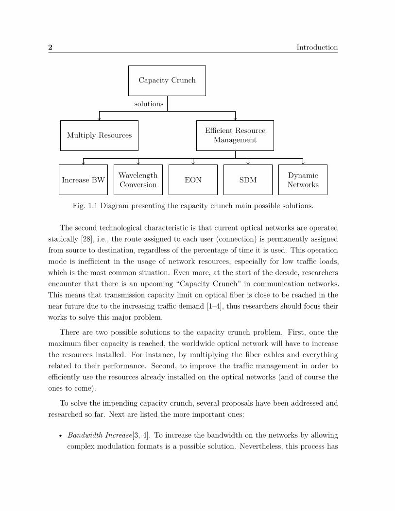
Fig. 1.1 Diagram presenting the capacity crunch main possible solutions.
The second technological characteristic is that current optical networks are operatedstatically [28], i.e., the route assigned to each user (connection) is permanently assignedfrom source to destination, regardless of the percentage of time it is used. This operationmode is inefficient in the usage of network resources, especially for low traffic loads,which is the most common situation. Even more, at the start of the decade, researchersencounter that there is an upcoming “Capacity Crunch” in communication networks.This means that transmission capacity limit on optical fiber is close to be reached in thenear future due to the increasing traffic demand [1–4], thus researchers should focus theirworks to solve this major problem.
There are two possible solutions to the capacity crunch problem. First, once themaximum fiber capacity is reached, the worldwide optical network will have to increasethe resources installed. For instance, by multiplying the fiber cables and everythingrelated to their performance. Second, to improve the traffic management in order toefficiently use the resources already installed on the optical networks (and of course theones to come).
To solve the impending capacity crunch, several proposals have been addressed andresearched so far. Next are listed the more important ones:
• Bandwidth Increase[3, 4]. To increase the bandwidth on the networks by allowingcomplex modulation formats is a possible solution. Nevertheless, this process has

3
limitations, since the modulation formats require a bigger bandwidth to properlytransmit and optical networks have a limited bandwidth capacity due the capacitycrunch. Therefore, this is not a realistic solution.
• Wavelength Conversion [31, 32]. This technology can help to overcome the capacitycrunch by adding more dynamism on the resource allocation, although it requires adynamic resource allocation (with a static operation is pointless). Nevertheless, itis not yet commercially available, and it will not be on the near future.
• Elastic Optical Networks [33–36]. This new paradigm allows to flexibly use thefrequency spectrum in order to attend different traffic needs adaptively, by givingonly the necessary bandwidth to each user (no more, no less). In order to achievethis, first the frequency spectrum is divided on several frequency slots units (calledFSU) and, later, the FSU can be grouped to fulfill the bandwidth required totransmit each application. This has been an important topic of investigationnowadays, but still requires some research and development to be implemented.
• Space Division Multiplexing [37, 38, 4]. This approach, use in both mobile andfiber networks, proposes to divide the channels physically. In optical network it willmean to create different optical fibers, in order to reduce the energy consumption.For instance, fibers with more than one core, or annular fiber cores. etc. This isapproach is still in development, and requires some research to be available in thenear future.
• Dynamic Optical Networks [5, 39]. Another way to help overcome the inefficienciesof static networks consists of allocating the resources required by each user onlywhen there is enough data to transmit. The possible lack of resources to successfullytransmit a piece of information can happen because dynamic networks are designedbased on a statistical commitment: from one side, for economy reasons dynamicnetworks are designed with the minimum possible amount of resources; on the otherside, for effectiveness they are designed to avoid (or, more generally, to minimize)the occurrence of information losses due to lack of resources when needed (blocking).
From these possible solutions, dynamic optical networks is the one closer to beimplemented, since the technology to migrate current networks is already available.Consequently, this thesis addressed this type of networks.

4 Introduction
On dynamic networks, to achieve a balance between the previously mentioned twoopposite goals (network savings, and quality of service), the network must be designed sothat the blocking probability of any connection is less than or equal to a given thresholdor bound, seen as a parameter of network design, which is usually a value close to 0. Thiscan be refined by looking for a design where each connection c must have a blockingprobability BPc less than a given bound βc, so, a specific restriction for each connection.In this way, we can give more or less importance (or priority) to some of the connections.
The network cost definition can be addressed as an economic and commercial pointof view. For example, representing the cost of how many optical fibers are needed onthe network, taking into account how many wavelengths each fiber can handle. However,this approach is highly volatile, since it quickly changes overtime, due the fast technologygrowth and commercial strategies. Hence, to measure the network cost in a stable andrepresentative way, we choose to use the number of wavelengths on the network, in asimilar way as in most works in literature [9, 5, 40, 41]. This is because the cost ofmany components in an optical network is strongly affected by this parameter. In fact, itdetermines how many infrastructure resources are needed on the network to achieve thenetwork operation. Moreover, if the number of wavelengths required increases by anyreason, the cost of the network components may be maintained or must be increased.This means that the economic network cost is a non-decreasing function of the networkcost measured as the number of network wavelength.
To design dynamic optical networks is necessary to solve several technical problems.Figure 1.2 presents the most important problems that need to be solved in order todesign dynamic WDM networks taking into account the main services they must provide.Notice that each problem is dependent of the previous problem (in the figure, the onebelow), and the complete solution of all the problem can be address as the Routing,Wavelength Assignment and Wavelength Dimensioning problem considering Fault Tol-erance (R&WD+FT problem), while guaranteeing a maximum blocking probabilitypredefine in the Service Level Agreement. Let us now describe each one of them.
Blocking Probability This measures the chance that any user can not transmit overthe network due to the lack of resources [10, 9]. As previously mentioned, dynamic opticalnetwork designers must achieve a balance between two contradictory objectives. On oneside, to minimize the network resources required, and on the other side, to guarantee a

5
FAULT TOLERANCE
ROUTING
WAVELENGTH DIMENSIONING
WAVELENGTH ASSIGNMENT
BLOCKING PROBABILITY
R&WAD+FT PROBLEMS
Fig. 1.2 Diagram presenting some of the main problems in Optical Network Design.
quality of service threshold to each user. In this context, the quality of service is measuredas the blocking probability. In consequence, the blocking probability is an importantparameter used to design (and evaluate) dynamic WDM optical networks.
Wavelength Assignment (WA) This means to define a wavelength to each user inorder to successfully communicate each source destination pair of nodes [10, 7, 9]. Thisproblem changes on static and dynamic networks. A static operation requires only onewavelength assignment previous network operation, since then do not change over time.However, on dynamic networks this problem has to be solved each time a user wantsto transmit, due to the system operation. By solving this problem on a network with

6 Introduction
wavelength continuity constraint becomes even harder to solve, due to the fact than thewavelength chosen has to be available in all the links belonging to the users path.
Wavelength Dimensioning (WD) It must also be determined how many wavelengthsshould be assigned to each link of the network, in order to achieve the compromise betweenefficiency and cost previously described [9, 18]. As many works on the literature, weassumed each connection needs one wavelength at each link it uses, in order to transportits content.
Routing (R) This is a basic component of the network operation: every connection isdefined by a pair of nodes in the network, the source and the destination, and for each suchpair the designer must assign a route to be followed by the data to be transmitted [10, 7, 9].
Fault Tolerance (FT) A major problem to be addressed is to ensure that the networkis still able to provide its transmission service after the failure of one or more of itslinks [42, 30, 43]. The solution to this problem consists of allowing the necessaryinfrastructure to rapidly re-establish communication between all source-destination pairsof nodes affected by these link failures. In addition, it is desirable that the method takesinto account any possible fault tolerance scenario in the network.
The recently described problems have a major economic, technique and scientificimportance, since any improvement will change the optical network infrastructure. Thissituation opens an opportunity to provide a meaningful contribution in actual networks,enabling to migrate from static to dynamic network operation. In practical terms, thiswill allow to highly increase the network capacity, in the sense of traffic demands, butwith a very low investment.
In consequence, this thesis has two main objectives:
1. First, to provide a fast, simple and accurate analytical model to measure eachuser blocking probability in WDM optical networks with wavelength continuityconstraints.
2. Next, thanks to the previous model, to jointly solve the most important technologicalproblems in dynamic optical networks presented in Figure 1.2. These are Routing,Wavelength Assignment, Wavelength Dimensioning, and Fault Tolerance.
7
The remainder of this thesis is as follows:
• In Chapter 2 we present an analytical model to evaluate the blocking probability indynamic WDM optical networks with wavelength continuity constraint taking intoaccount heterogeneous traffic.
• Chapter 3 contains a novel method to jointly calculate the number of wavelengthsneeded on each network link (Wavelength Dimensioning) when providing a novelwavelength assignment strategy called “Fairness Policy”, so that the blockingprobability of each user is lower than a certain pre-specified threshold (which is adesign parameter of the network).
• Next, in Chapter 4 we propose a new technique to simultaneously determine: theset of routes enabling each network user to transmit; the wavelength assignmentstrategy to be used; and the wavelength dimensioning necesarry on each networklink, while, again, guaranteeing a predetermined minimum quality of service.
• Chapter 5 includes a fault tolerance capacity on the previous solution, thus pre-senting a novel methodology to jointly solve the Routing, Wavelength Assignment,Wavelength Dimensioning and adding fault tolerance to the network to any set oflinks failure scenario.
• Finally, the conclusions of this thesis are given in Chapter 6.
Due to the fact that nowadays there is not enough resource savings to compensate thecomplexity introduced to the network when operating dynamically [5], we hope to achievea progress on the state of art that will finally enable the telecommunication companies tomigrate optical networks from the current static operation, to a dynamic one. In thisway, the enterprises using this technology will offer a significantly major number of user,with basically the same infrastructure installed.
Publications
In summary, the publications made during this thesis period are:
8 Introduction
Journals
[41] R. Vallejos and N. Jara. Join routing and dimensioning heuristic for dynamic WDMoptical mesh networks with wavelength conversion. Optical Fiber Technology, 20(3),2014.
[53] R. Vallejos, J. Olavarría, and N. Jara. Blocking evaluation and analysis of dynamicWDM networks under heterogeneous ON/OFF traffic. Optical Switching and Networking,20, 2016.
[81] Nicolás Jara, Reinaldo Vallejos, and Gerardo Rubino. Blocking Evaluation andWavelength Dimensioning of Dynamic WDM Networks Without Wavelength Conversion.Journal of Optical Communications and Networking, 9(8):625, 2017.
[117] Nicolás Jara, Reinaldo Vallejos, and Gerardo Rubino. A method for joint routing,wavelength dimensioning and fault tolerance for any set of simultaneous failures ondynamic WDM optical networks. Optical Fiber Technology, 38:30–40, 2017.
Conference
[82] N Jara, R Vallejos, and G Rubino. Blocking evaluation of dynamic WDM networkswithout wavelength conversion. In 2016 21st European Conference on Networks andOptical Communications (NOC), pages 141–146, 2016.
[83] Reinaldo Jara, Nicolas; Rubino, Gerardo; Vallejos. Blocking Evaluation of dynamicWDM networks without wavelength conversion. In 11ème Atelier en Evaluation dePerformances, Toulouse, France, 2016.
[87] C Meza, N Jara, V M Albornoz, and R Vallejos. Routing and spectrum assignmentfor elastic, static, and without conversion optical networks with ring topology. In 201635th International Conference of the Chilean Computer Science Society (SCCC), pages1–8, oct 2016.
[118] N. Jara, G. Rubino, and R. Vallejos. Alternate paths for multiple fault tolerance onDynamic WDM Optical Networks. In IEEE International Conference on High PerformanceSwitching and Routing, HPSR, volume 2017-June, 2017.

Chapter 2
Blocking Evaluation of DynamicWDM Networks
2.1 Introduction
The rapid increase in demand for bandwidth on existing networks has caused a growth inthe use of technologies based on WDM optical infrastructures [28, 44]. Currently, thistype of network is operated statically [28], i.e., the resources used by a connection (user)is permanently assigned from source to destination. This type of operation is inefficientin the usage of network assets, specially for low traffic loads, which is the most commoncase.
One way to help overcome these inefficiencies is to migrate these communicationinfrastructures to networks working dynamically. This operation mode consists in allo-cating the resources required only when the user has data to transmit. A possible lackof resources to successfully transmit can then happen, because dynamic networks aredesigned to save costs using the less possible amount of resources, and simultaneouslyto be effective (low burst losses). To achieve a tradeoff between these two contradictoryaspects, the network must be designed such that the connection blocking probability isless than or equal to a design parameter β. The evaluation of the real blocking probabilityachieved allows to determine whether or not each network user (each connection) is beingtreated with the required quality of service. As a result, the blocking probability is one of
10 Blocking Evaluation of Dynamic WDM Networks
the main parameters that has been used to evaluate the performance of dynamic WDMoptical networks [9].
In general, the blocking probability is evaluated through simulation [6, 7, 5]. Thereason is that the exact (numerically speaking) computation of this metric is most ofthe time out of reach, because of the complexity of the analysis, the combinatorialexplosion problem, etc. Nevertheless, simulations are in general very slow compared withthe solution obtained following a mathematical approach [8]. The evaluation speed isrelevant, because when solving problems of higher order (e.g. concerning routing or faulttolerant mechanisms), it is in general necessary to calculate the blocking probability alarge number of times. Thus, a fast and accurate mathematical computational method isextremely useful. However, to obtain a mathematical procedure with such characteristicsis a difficult task, due to important aspects to take into account while modeling, suchas: traffic load, wavelengths capacity, wavelength continuity constraint (because thenetwork operates without wavelength conversion), network topology, etc. Therefore,several hypotheses are typically introduced to simplify the model in order to facilitate itsanalysis.
One of these hypotheses is the homogeneous load assumption. Many works assumethat the traffic load offered by each connection to the network is statistically the same [45–52]. This hypothesis strongly simplifies the modeling, but it does not adequately representthe operation of optical networks (or computer networks in general), because the offeredtraffic is usually very heterogeneous. This is relevant since replacing each of the sourcesby the average of all of them can significantly modify the performance metrics of thesystem [53]. This underlines the interest in including the traffic load heterogeneity onthe network mathematical models used. In [54] a model based on the Erlang-B formulais proposed with the purpose of evaluating the link blocking probability. This modelallows different traffic loads on each network link, but since it is based on the Erlang-Bformula, the individual loads don’t appear in the solutions (only their sums do), and thus,it suffers from the same limitations as when the homogeneous assumption is used.
Another commonly used hypothesis is the Poisson traffic assumption, shared by themajority of papers published so far [55, 45–47, 54, 48, 49, 56, 50–52], which greatlysimplifies the mathematical evaluation. However, a Poisson process is not representativeof the real traffic in optical networks, for several reasons. For instance, the rate of theoffered traffic in a given link varies significantly over time, because it is sensitive to the

2.1 Introduction 11
number of connections that are not currently transmitting. Another way of using thePoisson modeling was proposed in [50, 46, 45] where the network is split into severallayers (one for each wavelength). The blocked traffic in one layer is overflowed to thenext. This overflowed traffic its not Poisson (it is bursty), therefore the authors usethe Fredericks and Hayward’s approximation [57, 58] to transform the bursty overflowedtraffic (non-Poisson) into a Poisson flow. The solving procedure then applies the Erlang-Bformula separately at each layer to evaluate its blocking probability. This formula canbe used on queuing systems where the arrival rate does not change with time, whichhappens when there is a huge number of connections. However, in an optical networkthe total number of users that can share a network link is low, and the arrival rate (onany instant and any network link) depends on the number of active connections passingthrough the link. Then, the arrival rate changes significantly over time, making thismodel inadequate.
In this chapter we propose a new approach to evaluate the blocking probability (of burstlosses) in dynamic WDM optical networks without considering wavelength conversion andwith heterogeneous traffic. The method is called Layered Iterative Blocking ProbabilityEvaluation, LIBPE in the text. It takes into account the bursty nature of the offeredtraffic, by modeling the sources with ON-OFF processes. Our technique obtains veryaccurate results in comparison to those achieved by simulation, with computational speedorders of magnitude faster.
We illustrate the use of our technique for calculating the number of wavelengths onevery network link, that is, for dimensioning the WDM network. The final networkdimensioning results show that the proposed method obtains the same results as theones obtained by simulation (which in general are based on the sequential execution ofsimulation experiments), but much faster (e.g. between 103 and 104 times faster).
The remainder of this chapter is as follows: In Section 2.2 we use a layer-basedstrategy to evaluate the blocking probability. Section 2.3 presents some numericalexamples. Then, Section 2.4 presents the dimensioning method and the obtained results.Finally, conclusions are given in Section 2.5.
12 Blocking Evaluation of Dynamic WDM Networks
2.2 Blocking evaluation strategy
The network is represented by a directed graph G = (N ,L), where N is the set ofnetwork nodes and L is the set of unidirectional links (the graph’s arcs), with respectivecardinalities N and L. The set of connections (or users) C ⊆ N 2, with cardinality C, iscomposed by all the source-destination pairs with communication between them, togetherwith the route followed by the data.
To represent the traffic between a given source-destination pair an ON-OFF model isused. In works such as [59], it has been demonstrated that the blocking probability ondynamic networks is mainly affected by the mean times tON y tOFF , and is practicallyinsensitive to the specific distribution of such times. In fact, in [60], the sensitivity ofthe blocking probability in dynamic networks on the blocking probability was studiedin such networks. That work concluded that, for practical purposes, we can considerthis probability as insensitive to the specific distribution of tON y tOFF . Consequently, torepresent the times of formation and transmission of bursts, our work uses only the meanvalues of those times.
Consider connection c. During any of its ON periods, whose average length is tON c,the source transmits at a constant transmission rate. During an OFF period, withaverage length tOFF c, the source refrains from transmitting data. We use the notationτc = tON c + tOFF c, and call it the average length of a cycle for connection c. For a givenuser, we assume that the lengths of ON (respectively OFF) periods are i.i.d. randomvariables, and that both sequences are independent of each other.
When traffic sources are ON, they all transmit at the same rate, determined by theused technology, that to simplify the presentation will be our rate unity. Consequently,the traffic load for connection c, denoted by ϱc, given by the following expression,
ϱc = tON c
tON c + tOFF c
, (2.1)
is also the mean traffic offered by connection c.
Let R = rc | c ∈ C be the set of routes that enable communication among thedifferent users, where rc is the route associated with connection c ∈ C. To simplify theexplanation, we assume for the moment that every link ℓ ∈ L has a same number W of
2.2 Blocking Evaluation Strategy 13
wavelengths associated with, but keep in mind that our method allows different numberof wavelengths on each network link (see at the end of Section II, paragraph a).
Let the W available wavelengths be numbered 1, 2, . . . , W . The network basicallyoperates as follows. Upon the arrival of a connection request to destination d, say byuser c, the source s will attempt to transmit on the first wavelength w = 1 on thepredetermined fixed path from node s to node d, by assuming a “first fit” wavelengthallocation method. The request is accepted if wavelength 1 is available on all the linksbelonging to the predetermined fixed path (wavelength continuity constraint), that is, onroute rc. Otherwise, the same request is offered to the next wavelength (w = 2). Theprocess continues in the same way, until there is some wavelength available on all the linksof the path, or until the W wavelengths have been considered and none was availablealong the path. In the first case, the node s transmits its information to d through theavailable wavelength, and in the last case, the request is blocked (lost).
Given the complexity of the exact evaluation of the blocking probability consideringall the aspects described before, we developed a strategy to obtain an accurate whilelight cost approximate computational scheme. Note that one of the most importantaspects to consider is the wavelength continuity problem, because there is no wavelengthconversion capability. This means that when a connection transmits, it must use thesame wavelength on each link that belongs to its route. We explain below the differentsteps of the LIBPE procedure.
2.2.1 Auxiliary sequence of networks
Observe that, from the vocabulary point of view, we can consider that the network isactually composed of W networks operating “in parallel”, with the same topology asthe original one, which we denoted by G, but where each link has a single wavelengthassociated with (that is, a capacity equal to 1). We will see this set of networks as asequence ⟨ G1,G2, . . . ,GW ⟩ and say that these auxiliary networks are different “layers”of G. Moreover, the single wavelength associated with each link in Gw is precisely the onehaving number w. Then, an arriving connection will look for room in layer 1 first, thatis, in network G1, if this fails, in G2, and so on, until it finds available capacity in one ofthe W layers, or until all of them block it.

14 Blocking Evaluation of Dynamic WDM Networks
The technique proposed in this work will then follow a decomposition approach: eachlayer will be analyzed in isolation, but its parameters will depend on what happens onthe other layers. The heuristic mentioned in the abstract appears in the way these twoelements (solving for a layer and using the dependencies between them) are treated.
To take into account the interaction between the W auxiliary networks we will establisha dependency between the mean lengths of the OFF periods associated with the sources.That is, the traffic offered to the different layers in the analysis process will (naturally) bedifferent for each one, and its calculation will take into account the different ways wherewhat happens with a wavelength impacts the traffic that will arrive to another one.
In the following, we describe the procedure in detail, which constitutes the maincontribution of the chapter.
2.2.2 Network analytical model when W = 1
Since the network is divided into a sequence of W networks/layers where each link hasnow capacity 1, we consider first the case of W = 1. With this, we have a method tosolve any of the Gw networks generated on the network division with link capacity equalsto 1. Fix a link in the network, say link ℓ. Some connections (at least one) use this linkin their routes, some don’t. Denote by Tℓ the number of connections using ℓ, and assumethat, once ℓ fixed, we renumber the connections so that those using link ℓ are 1, 2, . . . , Tℓ.Observe that link ℓ can be either free, or busy transmitting a burst from connection c,c = 1, 2, . . . , Tℓ.
Assume the system is in equilibrium, and denote by BLc,ℓ the blocking probability ofconnection c at link ℓ, that is, the probability that a burst of connection c arriving atlink ℓ finds it busy. To evaluate it, assume Markovian conditions, that is, Exponentiallydistributed burst generation times and Exponentially distributed burst transmission times,with respective rates λc and µc, with the usual independence conditions. The servicerate µc is simply µc = 1/tON c. For the arrival rate, observe first that when the link endstransmitting a burst, all the Tℓ connections (including the one that just transmitted) arein the OFF part of their cycles (this is because we are dealing with a loss system). So,when entering state 0, we have Tℓ exponential clocks competing, the c-th one with anexponentially distributed time length having parameter 1/tOFF c. So, λc = 1/tOFF c. Thecontinuous time stochastic process Z = Z(t), t ≥ 0 on the state space 0, 1, 2, . . . , Tℓ,

2.2 Blocking Evaluation Strategy 15
0
2
1
. ..
Tℓλ1
λ2
λTℓµ1
µ2
µTℓ
Fig. 2.1 Markov chain modeling the occupation of a given link in a network where all linkshave only one wavelength. There are Tℓ connections using the link. State c means thatconnection c is using the link, c = 1, 2, . . . , Tℓ. State 0 means that the single wavelengthof the link is available. Arrival rate of a burst of connection c: λc = 1/tOFF c. Service rate(by the link) of a burst of connection c: µc = 1/tON c.
representing the state of the link at time t, where Z(t) = 0 if link is idle at t, is thenMarkov (see Figure 2.1). A straightforward analysis of this Markov chain gives its steadystate distribution
(π0, π1, . . . , πTℓ
). The equilibrium equation of state c ∈ 1, 2, . . . , Tℓ is
πc · µc = π0 · λc. (2.2)
This immediately leads to
πc = φc
1 + φ, c = 1, 2, . . . , Tℓ, π0 = 1
1 + φ, (2.3)
where φc is the ratio φc = λc/µc = tON c/tOFF c and φ is the sum φ = φ1 + · · · + φTℓ.
Observe that, in terms of loads, we have φc = ϱc/(1− ϱc), since ϱc = λc/(λc + µc).
It is immediate to see that the equilibrium distribution (2.3) doesn’t depend onthe distribution of ON periods, that is, it doesn’t change if the ON periods have anyother distribution with finite expectation if this expectation is equal to 1/µc for user c.The reason is that any state i = 0 has only one successor (state 0), so, the model’sstationary distribution doesn’t change if we set the distribution of any of these holdingtimes to another distribution with the same mean (see, for instance, [61, Prop. 4.8.1] onsemi-Markov processes). Here, for simplicity in the presentation, we assume ExponentialON times.
The blocking probability BLc,ℓ is the ratio between the probability of a connection c
request being blocked for lack of resources and the probability of the union of all possible

16 Blocking Evaluation of Dynamic WDM Networks
scenarios when connection c wants to transmit. It can also be derived marking connection c
arrivals and analyzing the chain embedded at the marked transition epochs. The result is
BLc,ℓ = 1− π0 − πc
1− πc
= φ− φc
1 + φ− φc
. (2.4)
Since we are considering this evaluation on any of the Gw networks, we can conclude thatthe link blocking probability on the w-th network BLw
c,ℓ is equal to the one obtained onequation (2.4) considering the Gw network values tON and tOFF .
The blocking probability of connection c, with c ∈ C, on network Gw, that is, theprobability that a burst of connection c arriving at Gw finds at least one link busy in itsroute, can be then approximated by means of the typical link independence assumption,that is, by assuming that the states of the links in the network (or just in the route) areindependent of each other. This gives
BC wc = 1−
∏ℓ∈rc
(1− BLw
c,ℓ
). (2.5)
This independence assumption is not realistic in this highly competitive context wheremany connections can be often trying to access simultaneously the same resources (thisis called “Streamline Effect” in [62]). Moreover, remember that in the first Gw networks,with w close to 1, we are considering the border case where resources are really scarce(there is only one wavelength per link, and several users trying to use it). To improvethe quality of the approximation, we use the fixed point method proposed by Kelly [63]:once BC c, for all connections c, is computed, we modify the arrival rate λc by replacingit with the value λ′
c = λc(1−BC c). Then, we recompute a new blocking probability BC ′c
for all c, and we repeat the process until an appropiate convergence criteria is satisfied.
2.2.3 Networks interaction
Now that every layer performance can be evaluated using the scheme described in 2.2.2,we need to take also into account the interaction between the W networks G1, . . . ,GW .This interaction will be captured through new values characterizing the ON-OFF arrivalprocesses of the different connections on each network Gw. For this purpose, let us denoteby tONc,w and tOFFc,w the average values of ON and OFF periods for connection c innetwork Gw. Regarding tONc,w , since it is the time used by source c to transmit, it will be

2.2 Blocking Evaluation Strategy 17
Fig. 2.2 Time Equivalence Diagram. This figure shows every possible scenario where theuser 1 can be accepted or blocked when making a connection request. The network has4 users and a link’s capacity of 3 wavelengths. The upper half (above the dotted line)corresponds to each one of the 3 wavelengths showing the real tOFF 1 and tON 1 seen oneach wavelength by the user 1 and the lower part (bellow the dotted line) shows how theuser 1 times are taking place.
kept equal to the initial data tONc . In other words, the dependencies between layers will becaptured only by the tOFFc,w values and for all source c and wavelength w, tONc,w = tONc .
As an example, Figure 2.2 shows the time system diagram seen by user 1 when thereare 4 users and a link network capacity of 3 wavelengths (we have 3 auxiliary networksnamed G1, G2 and G3). The upper part (first 3 horizontal lines of the figure), shows howthe connections use the wavelengths resources, and how user 1 sees them work on anywavelengths separately in different scenarios, represented by its tON and tOFF . The lowerpart (under the dotted horizontal line) shows how user 1 destination node “sees” theoverall transmission time. Every arrival is marked with a vertical arrow. If the connectionrequest is blocked on a wavelength, then an X appears at the bottom of the arrow, and ifthe connection is accepted a block corresponding a transmission time (tON ) appears. Asmentioned before, wavelength allocation is First Fit as can be seen on the diagram.

18 Blocking Evaluation of Dynamic WDM Networks
The heart of our procedure concentrates then on those dependencies between layers,which are of three types, informally described below and represented on the TimeEquivalence Diagram shown on figure 2.2. The precise way in which these interactionswill be taken into account in the equations will be explicitly presented.
• Sequential dependency: when a request from connection c is accepted at layer Gw,the next layers will not receive it. In other words, a wavelength in the sequence receivesa request from connection c only if it is blocked in every previous wavelengths in thesequence. Therefore, tOFFc,w′ will grow by the quantity τc = tOFFc + tONc in everyw′ > 1, for each request transmitted on the wavelengths previous to w′. This can beseen on figure 2.2, where the second wavelength will receive a request only when thesame connection request is blocked on the first wavelength..
• Backward dependency: After connection c is blocked on network G1 and acceptedin any of the next wavelengths, the next transmission request (in G1) of connection c
will occur after one transmission period -because the first request was accepted- andone idle period (mean length tOFFc) to collect new data to transmit. Therefore, allblocked connections in network G1, but accepted on any of the next networks Gw,w > 1, make tOFFc,1 grow by τc. Notice that this does not only affects only on the firstlayer G1, but every layer in the network. But it is enough to consider this dependencyonly on G1, because the sequential dependency will spread this effect. This can beseen on figure 2.2, where user 1 next request time on the first wavelength increasesevery time user 1 is accepted on any other wavelength but the first.
• General blocking dependency: This considers the scenario when a connection c
request is blocked on every wavelength (every network Gw, for all w). In this case,connection c start again to collect new data to transmit (OFF period). Therefore, allblocked connections in the final network GW make the tOFFc,1 value increase by tOFFc .This can be seen in fig. 2.2 when the user 1 is blocked on every wavelength.
Let us go now through the details concerning the evaluation of tOFFc,w for all ws, con-sidering the dependencies just introduced. For this purpose, we will denote by BC w
c theblocking probability of connection c at layer Gw.
• First Wavelength (w = 1). On the first wavelength, that is, on the first layer G1,we take into account the last 2 dependencies. First, when connection c is blocked

2.2 Blocking Evaluation Strategy 19
on G1 and accepted in any of the next layers, it will have to wait an additionallydelay τc until trying to transmit again on G1 (Backward dependency). Second, if theconnection is blocked in every following wavelength, that is, in every layer, then theconnection starts again an OFF period (General blocking dependency). These factstranslates into the following relationship, by considering every possible scenario ina probabilistic way:
tOFFc,1 = tOFFc
+ 0 · (1− BC 1c)
+ τcBC 1c(1− BC 2
c)+ τcBC 1
cBC 2c(1− BC 3
c)+ · · ·
+ τc
(W −1∏k=1
BC kc
)(1− BC W
c )
+ tOFFc
(W∏
k=1BC k
c
).
(2.6)
The first term in (2.6) considers the source tOFFc of the connection c. The secondterm represents the probability of being accepted on the first wavelength, in whichcase the value of tOFFc,1 remains unchanged. The next terms correspond to the casesof connection c accepted at the next layers (w > 1), in which case the Backwarddependency applies. The very last term handles the case where the connection isblocked on every possible wavelength; in that case, the General blocking dependency.Now, (2.6) can be simplified into
tOFFc,1 = tOFFc
(1 +
W∏k=1
BC kc
)+ τc
∑1≤i≤W −1
(1− BC i+1c )
i∏k=1
BC kc . (2.7)
The last term in previous equation has a telescopic sum inside. This allows a furthersimplification:
tOFFc,1 = tOFFc + τcBC 1c − tON c
W∏k=1
BC kc . (2.8)
• Next wavelengths now. Observe first that layer Gw, for w > 1, will not have aconnection request from user c until this user is blocked on all previous layers. So,
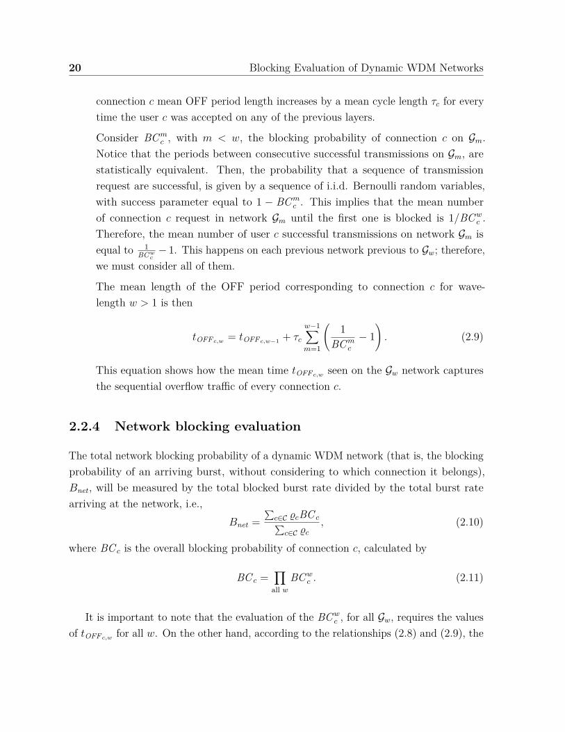
20 Blocking Evaluation of Dynamic WDM Networks
connection c mean OFF period length increases by a mean cycle length τc for everytime the user c was accepted on any of the previous layers.
Consider BC mc , with m < w, the blocking probability of connection c on Gm.
Notice that the periods between consecutive successful transmissions on Gm, arestatistically equivalent. Then, the probability that a sequence of transmissionrequest are successful, is given by a sequence of i.i.d. Bernoulli random variables,with success parameter equal to 1 − BC m
c . This implies that the mean numberof connection c request in network Gm until the first one is blocked is 1/BC w
c .Therefore, the mean number of user c successful transmissions on network Gm isequal to 1
BCwc− 1. This happens on each previous network previous to Gw; therefore,
we must consider all of them.
The mean length of the OFF period corresponding to connection c for wave-length w > 1 is then
tOFFc,w = tOFFc,w−1 + τc
w−1∑m=1
(1
BC mc
− 1)
. (2.9)
This equation shows how the mean time tOFFc,w seen on the Gw network capturesthe sequential overflow traffic of every connection c.
2.2.4 Network blocking evaluation
The total network blocking probability of a dynamic WDM network (that is, the blockingprobability of an arriving burst, without considering to which connection it belongs),Bnet, will be measured by the total blocked burst rate divided by the total burst ratearriving at the network, i.e.,
Bnet =∑
c∈C ϱcBC c∑c∈C ϱc
, (2.10)
where BC c is the overall blocking probability of connection c, calculated by
BC c =∏
all w
BC wc . (2.11)
It is important to note that the evaluation of the BC wc , for all Gw, requires the values
of tOFFc,w for all w. On the other hand, according to the relationships (2.8) and (2.9), the
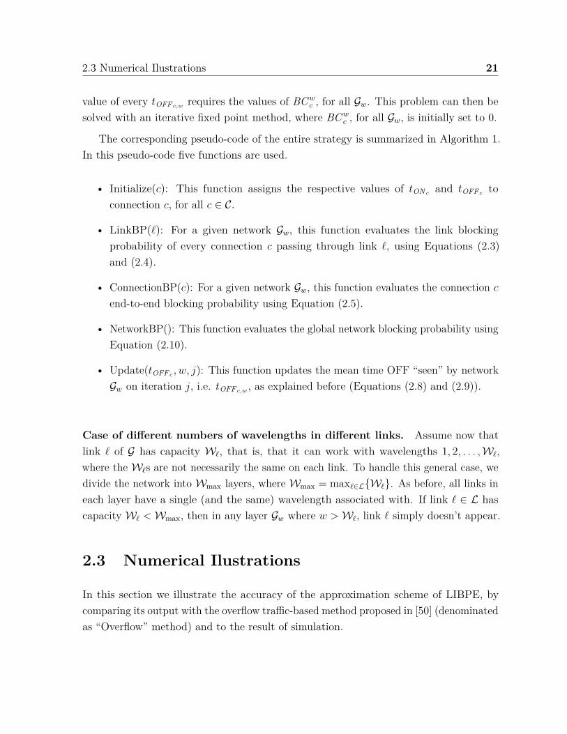
2.3 Numerical Ilustrations 21
value of every tOFFc,w requires the values of BC wc , for all Gw. This problem can then be
solved with an iterative fixed point method, where BC wc , for all Gw, is initially set to 0.
The corresponding pseudo-code of the entire strategy is summarized in Algorithm 1.In this pseudo-code five functions are used.
• Initialize(c): This function assigns the respective values of tONc and tOFFc toconnection c, for all c ∈ C.
• LinkBP(ℓ): For a given network Gw, this function evaluates the link blockingprobability of every connection c passing through link ℓ, using Equations (2.3)and (2.4).
• ConnectionBP(c): For a given network Gw, this function evaluates the connection c
end-to-end blocking probability using Equation (2.5).
• NetworkBP(): This function evaluates the global network blocking probability usingEquation (2.10).
• Update(tOFFc , w, j): This function updates the mean time OFF “seen” by networkGw on iteration j, i.e. tOFFc,w , as explained before (Equations (2.8) and (2.9)).
Case of different numbers of wavelengths in different links. Assume now thatlink ℓ of G has capacity Wℓ, that is, that it can work with wavelengths 1, 2, . . . ,Wℓ,where the Wℓs are not necessarily the same on each link. To handle this general case, wedivide the network into Wmax layers, where Wmax = maxℓ∈LWℓ. As before, all links ineach layer have a single (and the same) wavelength associated with. If link ℓ ∈ L hascapacity Wℓ <Wmax, then in any layer Gw where w >Wℓ, link ℓ simply doesn’t appear.
2.3 Numerical Ilustrations
In this section we illustrate the accuracy of the approximation scheme of LIBPE, bycomparing its output with the overflow traffic-based method proposed in [50] (denominatedas “Overflow” method) and to the result of simulation.

22 Blocking Evaluation of Dynamic WDM Networks
Algorithm 1 Layered Iterative Blocking Probability Evaluation1: procedure LIBPE2: for each c ∈ C do3: ⟨tONc , tOFFc⟩ ← Initialize(c)4: end for5: j ← 16: repeat7: for w ← 1 to Wmax do8: for each c ∈ C do9: tOFFc,w(j) ← Update(tOFFc , w, j)
10: end for11: for each ℓ ∈ L do12: BLi
ℓ,w(j) : for all i ← LinkBP(ℓ)13: end for14: for each c ∈ C do15: BC w−1
c (j) ← ConnectionBP(c)16: end for17: end for18: j ← j + 119: until (BC w
c (j),∀c ∈ C converges)20: Bnet ← NetworkBP()21: end procedure
The simulation results where obtained by an event based Monte Carlo simulation.The simulation was made to represent how dynamic optical networks perform, i.e. itdoes not use a layer based approach to operate, it emulates the network work withoutwavelength conversion. Since we wanted to have a good idea about the accuracy of theapproximation, we stopped the simulation when we had a statistical relative error onthe targets (the global network blocking probabilities) less than 5%, a pretty stressingobjective. We are considering here a typical network performance evaluation processwhere the systems are considered in equilibrium, so, the simulation results were obtainedby removing the initial transient phase, that is, using the concept of warm-up time. Foreach simulation, enough bursts were generated in order to accomplish a 95% intervalconfidence.
In real optical infrastructures, the lengths of ON periods are proportional to the burstsize, which depends on the burst aggregation mechanism [64, 65]. These bursts havea maximum size and in this context where resources are scarce, the maximum burst

2.3 Numerical Ilustrations 23
Fig. 2.3 Mesh networks evaluated. Each edge on the networks are bidirectional, so thenumber of links L refers to unidirectional arcs on each graph. The parameter d is ameasure of density: if the graph has L arcs (the picture shows L/2 edges) and N nodes,then d = L/
(N(N − 1)
).
size will in general be reached. This suggests that a constant length ON period is muchmore realistic than an Exponentially distributed one. Thus, we used the same data butchanged the length in time of the ON periods of every connection, from random andExponentially distributed to deterministic, that is constant ones.
In the experiments we compared the outputs of LIBPE method with simulationresults using four different real mesh topologies. Figure 2.3 shows these topologies andsome of their parameters: number N of nodes, number L of links (the arcs of the graph,that is, twice the number of edges that are drawn in the picture) and network densityd = L/
(N(N − 1)
).

24 Blocking Evaluation of Dynamic WDM Networks
Figure 2.4 shows the results for the different graphs. The parameter tON was set to10 ms and tOFF was varied, in order to obtain different values for the traffic load, ϱ, inthe range [0.1...0.9].
Regarding the Overflow method [50], as explained on Section 2.1, it is based by theoverflow traffic analysis used on ITU’s teletraffic engineering [57]. In this case, the networkis split into several layers (one for each wavelength) where the blocked traffic in one layeris overflowed to the next, and uses the Fredericks and Hayward’s approximation [57, 58]to transform the bursty overflowed traffic (non-Poisson) into a Poisson flow. Then, tosolve each layer blocking probability applies the Erlang-B formula.
To compare our method with the Overflow method, we compared the outputs ofLIBPE and the Overflow method with simulation results using four different real meshtopologies presented in Figure 2.3.
2.3.1 Analysis of the results
In the experiments, our method always gave results very close to those coming fromsimulations, as illustrated in the examples used in the chapter. We see that our heuristicprocedure LIBPE is extremely accurate, and the results reported show that LIBPE isvery robust with respect to the model assumptions concerning the length of ON periodsat the sources, the mechanism in which we capture the overflow between network layers,the blocking probability evaluation method at each layer, and using Kelly’s technique toconsider the Streamline effect. Our results also show that LIBPE outperforms significantlythe standard Overflow method.
If we compare the LIBPE and Simulation sets of curves composing Figure 2.5, it’shard to see any difference between them (in a logarithmic scale, as shown on Figure 2.5).Then, to make a zoom on this aspect of the work, consider the case of the UKNet topologywith 10 wavelengths per network link, when the load of all connections is 0.3. In thiscase we observed the largest differences between LIBPE and simulation. Our methodobtains a global network blocking probability of 9.56 · 10−2, and using simulation, theestimation was equal to 5.78 · 10−2. At an opposite situation, consider the Eurocorenetwork topology with 3 wavelengths per link and, again, a traffic load of 0.3. LIBPEobtains Bnet = 4.56 ·10−2; and simulation led to a global blocking probability of 4.41 ·10−2.As a supplementary and positive comment, we always observed that LIBPE evaluates the
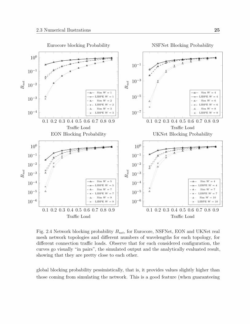
2.3 Numerical Ilustrations 25
0.1 0.2 0.3 0.4 0.5 0.6 0.7 0.8 0.910−4
10−3
10−2
10−1
100
Traffic Load
Bne
t
Eurocore blocking Probability
Sim W = 1LIBPE W = 1
Sim W = 2LIBPE W = 2
Sim W = 3LIBPE W = 3
0.1 0.2 0.3 0.4 0.5 0.6 0.7 0.8 0.910−7
10−5
10−3
10−1
Traffic LoadB
net
NSFNet Blocking Probability
Sim W = 4LIBPE W = 4
Sim W = 6LIBPE W = 6
Sim W = 8LIBPE W = 8
0.1 0.2 0.3 0.4 0.5 0.6 0.7 0.8 0.910−6
10−5
10−4
10−3
10−2
10−1
100
Traffic Load
Bne
t
EON Blocking Probability
Sim W = 5LIBPE W = 5
Sim W = 7LIBPE W = 7
Sim W = 9LIBPE W = 9
0.1 0.2 0.3 0.4 0.5 0.6 0.7 0.8 0.910−6
10−5
10−4
10−3
10−2
10−1
100
Traffic Load
Bne
t
UKNet Blocking Probability
Sim W = 4LIBPE W = 4
Sim W = 7LIBPE W = 7Sim W = 10
LIBPE W = 10
Fig. 2.4 Network blocking probability Bnet , for Eurocore, NSFNet, EON and UKNet realmesh network topologies and different numbers of wavelengths for each topology, fordifferent connection traffic loads. Observe that for each considered configuration, thecurves go visually “in pairs”, the simulated output and the analytically evaluated result,showing that they are pretty close to each other.
global blocking probability pessimistically, that is, it provides values slightly higher thanthose coming from simulating the network. This is a good feature (when guaranteeing
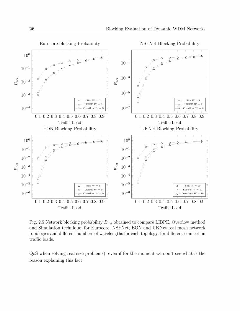
26 Blocking Evaluation of Dynamic WDM Networks
0.1 0.2 0.3 0.4 0.5 0.6 0.7 0.8 0.910−4
10−3
10−2
10−1
100
Traffic Load
Bne
t
Eurocore blocking Probability
Sim W = 3LIBPE W = 3
Overflow W = 3
0.1 0.2 0.3 0.4 0.5 0.6 0.7 0.8 0.910−7
10−5
10−3
10−1
Traffic LoadB
net
NSFNet Blocking Probability
Sim W = 8LIBPE W = 8
Overflow W = 8
0.1 0.2 0.3 0.4 0.5 0.6 0.7 0.8 0.910−6
10−5
10−4
10−3
10−2
10−1
100
Traffic Load
Bne
t
EON Blocking Probability
Sim W = 9LIBPE W = 9
Overflow W = 9
0.1 0.2 0.3 0.4 0.5 0.6 0.7 0.8 0.910−6
10−5
10−4
10−3
10−2
10−1
100
Traffic Load
Bne
t
UKNet Blocking Probability
Sim W = 10LIBPE W = 10
Overflow W = 10
Fig. 2.5 Network blocking probability Bnet obtained to compare LIBPE, Overflow methodand Simulation technique, for Eurocore, NSFNet, EON and UKNet real mesh networktopologies and different numbers of wavelengths for each topology, for different connectiontraffic loads.
QoS when solving real size problems), even if for the moment we don’t see what is thereason explaining this fact.

2.4 Summary and example of application 27
The main difference between LIBPE and simulation is the time required to obtain thenetwork blocking probability. For example, to generate the curves for the UKNet network,the mathematical method took less than a second, while the simulation procedures neededabout 6 hours in the same computer. The practical implication of this is that our methodcan be used as an engine internal to a real time decision system, or to assess networkperformance under different scenarios as a part of an optimization process.
2.4 Summary and example of application
2.4.1 Summary of the chapter’s proposal
In qualitative terms, the main characteristics of our approach are the following ones:
• Our method divides the network into W separated networks G1, . . . ,GW , that wecall layers, to handle the wavelength continuity problem. This allows designing anevaluation technique that decomposes the problem into two different procedures: onefor analyzing each layer in isolation, and the other one to interconnect what happensin the different networks. This approach leads to a significant simplification of theevaluation, compared to the effort in computing exactly the blocking probabilities,out of reach even for small networks because of the combinatorial explosion problem.
• To consider the overflowed traffic from a layer to the next, we modify the meanOFF time period for each connection (user) “seen” on each layer, considering theexistent dependencies between them.
• The Markov chain proposed to evaluate every link blocking probability on eachGw network considers an ON-OFF traffic, taking into account the mean OFF andON time periods “seen” on each network.
• Our method takes into account the fact that the blocking probability of a linkdepends on what happens with other links in the network (“Streamline Effect”).The majority of the connections pass through more than one link, which meansthat if a connection request is blocked in one of the first links of its route, therequest does not reach the following links of the route (the “downstream” links).
28 Blocking Evaluation of Dynamic WDM Networks
This phenomenon affects the load perceived by downstream links and thereforetheir blocking probabilities.
• The model allows to take into account heterogeneous traffic. This is importantbecause it represents reality more accurately than the usual homogeneous trafficassumption.
• Our methodology allows to obtain very accurate results in, say, less than a secondfor real mesh topologies.
2.4.2 Wavelength Dimensioning
We illustrate the use of the procedure proposed in this thesis to dimension the numberof wavelengths required on every network link, as a function of the offered traffic anda performance objective The latter typically consists in finding the capacity of thelinks such that the blocking probability BC c of each connection c does not exceed apredefined maximum tolerance value (typically agreed in the Service Level Agreementbetween carriers and customers). The number of wavelengths impacts significantly thenetwork cost, therefore an efficient dimensioning of every link in an optical network is ofparamount importance. Usually, the dimensioning of these networks has been done basedon simulation. The calculation speed is important, so the network designers may solvehigher order problems faster.
For different reasons, the usual dimensioning procedures consider homogeneity in thelinks’ capacities, that is, they look for a capacity W , the same on all links, such thatthe performance objective is reached; see for example [24, 66, 22, 23, 20]. Solving thisprocedure with different links’ capacities leads to a state space that grow exponentiallyin size. This means that solving this problem by simulation becomes hard. We willthen follow here the same approach, because this can facilitate further comparisons withexisting methods. The idea is simple: we are given the network topology and the offeredtraffic, and our tolerance value for the blocking probability of connection c, BC TARGET
c .We then initialize the network capacity W by value 1 and we evaluate the blockingprobabilities per connection BC 1, ..., BC C in two different ways, using simulation andby means of our analytical procedure (in order to be able to compare their respectivedimensioning and execution times); then, we check the condition “for all connection c ∈ C,

2.4 Summary and example of application 29
Network Topology BC TARGETc Method Cnet Execution Time(s)
Eurocore
10−6 AnHD 400 3.20 · 10−2
10−6 SimHD 400 3.98 · 102
10−3 AnHD 300 1.60 · 10−2
10−3 SimHD 300 2.28 · 102
NSFNet
10−6 AnHD 672 2.34 · 10−1
10−6 SimHD 672 1.21 · 103
10−3 AnHD 546 1.72 · 10−1
10−3 SimHD 546 7.25 · 102
EON
10−6 AnHD 1716 1.25 · 100
10−6 SimHD 1716 2.06 · 103
10−3 AnHD 1404 8.90 · 10−1
10−3 SimHD 1404 1.82 · 103
UKNet
10−6 AnHD 1872 1.62 · 100
10−6 SimHD 1872 2.37 · 103
10−3 AnHD 1560 1.03 · 100
10−3 SimHD 1560 2.11 · 103
Table 2.1 Computational time required to calculate the total number of wavelengthsCnet with the homogeneous dimensioning method based on simulation (SimHD) andthe proposed analytical procedure (AnHD). Both dimensioning algorithms considers themaximum connection blocking probability BC TARGET
c with values equal to 10−3 and 10−6,and are applied to Eurocore, NSFNet, EON and UKNet real mesh network topologies fora mean traffic load equal to 0.3. HD stands for Homogeneous Dimensioning, meaningthat all links have the same number of wavelengths associated with.
BC c ≤ BC TARGETc ”. If the condition is satisfied, we stop the algorithm. If not, we increase
W by 1 and we repeat the procedure.
Let us denote by AnHD the dimensioning procedure using our mathematical approachfor evaluating the blocking probabilities, as in Analytical Homogeneous Dimensioning;

30 Blocking Evaluation of Dynamic WDM Networks
and by SimHD the analogous method using simulation for the same evaluations, as inSimulation-based Homogeneous Dimensioning. Our goal is to verify the robustness of theapproach by checking that both algorithms will produce the similar values for W , andthe corresponding execution times.
The two dimensioning algorithms, AnHD and SimHD, were applied to different realmesh network topologies. Both algorithms where used in a PC Intel Core I7 with 16GB ofRAM and Windows 8 OS. Table 2.1 shows the computational time required to calculatethe total network cost Cnet = LW , where W is the capacity per link calculated by eachalgorithm applied to mesh network topologies, for values of BC TARGET
c equal to 10−3 and10−6, for a mean connection traffic load equal to 0.3.
In Table 2.1 it is clear that our method is very accurate. Indeed, in all scenariosevaluated the dimensioning procedure gave roughly the same results as the simulationmethod. Moreover, it is clear that AnHD has a very low execution time, which is between3 and 4 orders of magnitude smaller than the execution time of SimHD. For example, onthe network EON AnHD is 1648 and 2044 times faster than SimHD, when we consider amaximum blocking probability of 10−3 and 10−6 respectively.
2.5 Conclusions
In this chapter a new layer-based mathematical method called LIBPE for blockingprobability evaluation of dynamic WDM optical networks without considering wavelengthconversion and taking into account heterogeneous traffic is presented. Another feature ofour technique is that it considers that the sources are modeled by ON -OFF processes.This allows to take into account the non-uniform (bursty) nature of the traffic offered tothe links. The link blocking dependency is handled by means of the Kelly’s Reduced Loadmethod. By dividing the network into several layers, the wavelength continuity constraintcan be efficiently taken into account. The interactions between layers is consideredthrough the mean OFF periods seen on every network layer.
The results obtained have been compared with simulation and with another commonlyused method. The results of the proposed technique are accurate enough to closely matchthose obtained by simulation. By its analytical nature, our method allows to obtain the

2.5 Conclusions 31
blocking probability of the network in a fraction of a second. This is usually severalorders of magnitude faster than using simulation.
As an illustration of the calculating procedure, we report its use for wavelengthdimensioning providing a QoS guarantee on the connections’ blocking probability. Byusing our method, we can solve this problem 4 orders of magnitude faster than simulationon the scenarios presented. This is relevant, because allows the network designer to solveproblems of higher order several times, to adjust and improve the network designingprocedures, to further optimize costs or benefits with respect to other parameters, etc.
As in several procedures of this type, some mathematical aspects have not beenconsidered, namely the existence and unicity of fixed points, or the validity of theconvergence tests in the fixed point calculations. In future work we will explore theseissues, for instance by analyzing the potential use of Brouwer theorem and extensions forthe analysis of the fixed points, or the capabilities of different convergence tests. Ouronly claim here is the fact that in a large set of experiments, some of which are reportedhere, we never found any problem with these mathematical issues.


Chapter 3
Wavelength assignment anddimensioning
3.1 Introduction
A central issue in WDM optical networks is to choose which wavelength is going to beused by each connection (also called “user”) every time they want to transmit, denoted asthe “Wavelength Assignment” (WA) problem [9, 7, 10]. The solution of this problem ondynamic WDM optical networks is specially tricky when the network has not wavelengthconversion capabilities. This lack of wavelength conversion means when a connectionwants to transmit, the same wavelength has to be available on every link belonging tothe given connection route (end-to-end). In other words, there is a wavelength continuityconstraint. Notice that the chosen wavelength changes over time, since every time theuser request resources to send data the WA method searches an available wavelength onthe user route links. This problem has been vastly covered by´previous work [9, 7, 10–16].Next we present some of the most common heuristics proposed in the literature to solvethe WA problem:
• First Fit (FF) [16, 17, 12]. This is the most common and fastest method used todate. In this scheme the wavelengths are considered as a sequence. When searchingfor an available wavelength upon the arrival of a connection request, the searchstarts on the first wavelength in the sequence. The request is accepted if the first

34 Wavelength assignment and dimensioning
wavelength is available on all the links belonging to the predetermined user fixedpath. Otherwise, the same request is send to the next wavelength on the sequence.The process continues on the same way, until there is some wavelength availableon all the links of the path, or until all the wavelengths have been checked andnone was available along the path. This scheme performs well in terms of blockingprobability, and is preferred in practice because of its small computational overheadand low complexity. Additionally, it does not introduce any communication overheadbecause no global knowledge is required.
• Random Fit (RF) [10, 11]. This technique searches through every possible wave-length along the path as the previous scheme, but it selects the wavelength sequencerandomly, using any probability distribution (usually an uniform one). It willcontinuing doing so until there is a wavelength available to transmit on each linkalong the user’s route, or until every wavelength has been checked and none of themis available. This method does not require further information from the networkstatus, hence does not introduce any communication overhead as well.
• Most-Used (MU) [12, 11, 10, 67]. Also known as PACK, the MU scheme choosesthe wavelength that is most-used in the network. The performance of MU slightlyoutperforms FF [10, 14], doing a better job of packing connections into fewerwavelengths and conserving the spare capacity of less-used wavelengths; by doingso it maximizes the wavelengths usage. In order to obtain a solution it requiresglobal information to compute the most-used wavelength; therefore, it introducesadditional communication overhead.
• Least-Used (LU) [11, 68, 10]. Also known as SPREAD, this method selects the wave-length that is the least used in the network. By choosing the least-used wavelengthit seeks to balance the load among all the wavelengths. The performance of LU isworse than Random and the communication overhead; storage and computationcost are all similar to those in MU [14, 10].
To solve the WA problem, it is required to previously know how many wavelengthswhere assigned to the network links. Finding the number of wavelengths of the links iscalled the “Wavelength Dimensioning” (WD) problem [9]. The number of wavelengthsimpacts significantly the network cost, since it determines how many infrastructureresources are needed in the network to achieve the network operation [18]. Additionally,

3.1 Introduction 35
it greatly influences the network performance. Therefore an efficient dimensioning ofevery link in an optical network is of paramount importance.
To achieve an efficient Wavelength Dimensioning on dynamic networks, two con-tradictory objectives must be satisfied. On the one hand, it is necessary to diminishthe cost in infrastructure, thus the network cost; on the other hand, it is necessary toguarantee a certain level of quality of service to the network users, measured by the userblocking probability. In other words, the network is designed to offer a very low blockingprobability to the users (a value close to 0) and to simultaneously save meaningful networkresources.
To solve the Wavelength Dimensioning problem on dynamic networks without wave-length conversion, several studies have been proposed so far. They can be classified intwo different categories, as shown next:
• Approximations [69–72, 9]. These approaches provide an analytical insight of howmany wavelengths should be assigned to each network link. They allow to analyzethe wavelength dimensioning by providing a theoretical lower limit on the numberof wavelengths required [69, 70, 72]. Additionally, in Ramaswami (2009) [9] ananalytical lower bound is proposed, in which the dimensioning must be less thanthe static case scenario. The article also proposes an heuristic method to dimensioneach link capacity based on graph coloring, considering the maximum load scenario.This proposal does not take into account the quality of service given to the networkusers.
• Statistical method [12, 9]. This method calculates the number of wavelengths oneach link taking into account the quality of service given to each network connection,measured as the user blocking probability. To dimension the network, the procedureis carried out for a given value of the traffic load. The main goal of this techniqueis to calculate the minimum amount of wavelengths necessary to communicate allsource-destination pair of nodes, while guaranteeing a maximum blocking probabilityto each network user (close to 0). A standard procedure for assessing this problemhas been to assign the same number of wavelengths to each network link; see forexample [12, 19, 21, 25]. We call this procedure “Homogeneous Dimensioning”. Inthis case, initially the network links are allocated with 1 wavelength each (thisallocation results in a very high blocking probability); next, this value is sequentially
36 Wavelength assignment and dimensioning
increased by one at each network link, until the network blocking probability reachesa pre-established threshold value, typically evaluated by means of simulation [5, 16].
The Homogeneous Dimensioning is the most common method used to date [12, 19–27].However, these studies have failed to recognize that this procedure over-dimensionsthe network. The homogeneous dimensioning is suitable for those networks where therouting algorithm balances the traffic load across the links (i.e. all the network linkshave very similar levels of utilization). As this balanced-load routing is very muchused (e.g.[73, 74, 25]), this dimensioning technique would be appropriate for many cases.Nevertheless, it is not entirely possible to completely balance the network, due, in general,to the fact that the topologies are not symmetric and the traffic load is usually asymmetric.
Notice that, since the wavelength dimensioning has been usually solved by simulation,the time-consuming task involved does not allowed to explore every possible solution onthe dimensioning. For instance, to solve the dimensioning problem with different links’capacities, the number of different scenarios to be evaluated grows exponentially. Then,to solve this problem by simulation becomes even harder to obtain.
A long standing issue in optical networks has been to provide a certain quality ofcommunication to the network connections, despite the existence of different classes ofusers. This multi-class traffic occurs due to the existence of different priority users (or QoSrequirements) [75, 76], or of some mechanisms to intentionally drop non-compliant burstsin order to improve the network performance [77]. In spite of these observations, the usualwavelength assignment and dimensioning approach (First-Fit wavelength assignmentwith an homogeneous dimensioning procedure) does not take into account these issues.For instance, the first fit wavelength assignment scheme fails to consider classes ofusers, since it merely searches an available wavelength sequentially, without making anyclass distinction. On the other hand, in the homogeneous dimensioning, the number ofwavelengths assigned to the network links is usually defined by the user class with thestrictest QoS requirement, thus providing to the classes with a lower priority, a betterquality of service than the one requested on the SLA. In the context of OBS networks,several works [78–80] address a mechanism to provide an absolute differentiated serviceto each user class, improving the network performance. The mechanism is based on adynamic wavelength assignment, in which a wavelength sharing policy is proposed. Thispolicy allows to provide a strict end-to-end QoS for each network user. The authorsconsider a single link, and by using linear programming they calculate different thresholds
3.1 Introduction 37
to each connection passing through the link. These thresholds define a limited set ofwavelengths that the connections can use while attempting to transmit, according to theirQoS requirements. The method relies on previous dimensioning of the network, thus itrequires a proper dimensioning procedure to satisfy each connection QoS. Additionally,the OBS network context simplifies the problem, due there is not wavelength continuityconstrains allowing to address the problem on each link separately.
This chapter presents a new method to jointly define a policy to assign the wavelengthsto each network connection, and to calculate the number of wavelengths in DynamicWDM Optical Networks without wavelength conversion. To solve this problem, themethod contemplates that each network connection has a fixed route to transmit, definedprevious to the network operation. This new approach has two main differences withprevious strategies. First, it assigns a different number of wavelengths to each networklink (denoted as “Heterogeneous Dimensioning”), such that the blocking probability ofeach connection does not exceed a predefined maximum tolerance value (typically agreedin the Service Level Agreement between carriers and customers). Second, it proposesa new wavelength assignment policy called “Fairness Policy”. This policy provides toeach network user a quality of service (blocking probability) as close as possible to theone required in the SLA, since each connection may have different quality of servicerequirements. By doing so, the fairness policy allows to reduce the amount of wavelengthsrequired in the network.
Numerical results presented at the end of the chapter (Section 3.3) show that theproposed algorithm no only enjoys advantages of low complexity and ease of implemen-tation, but that it is also able to achieve much better performance (measured as thetotal number of wavelengths required on the network) than the homogeneous wavelengthdimensioning approach with a regular wavelength assignment scheme such as first-fit.
The remainder of this chapter is as follows: In Section 3.2 we present the FairHeterogeneous Wavelength Dimensioning method. Section 3.3 contains some resultsobtained by the proposed algorithm, which are compared with those obtained with thecurrent best methods in a set of different scenarios. Finally, the conclusions of the studyare given in Section 3.4.
38 Wavelength assignment and dimensioning
3.2 Wavelength Assignment and Dimensioning
This section contains the main contribution of the chapter. We present first the modelused and the associated assumptions. Then, we present the algorithm we found to solvethe problem of Wavelength Assignment and Dimensioning (WA&D).
3.2.1 Model and assumptions
The network topology is represented by a graph G = (N ,L), where N is the set ofnetwork nodes or vertices and L is the set of unidirectional links (the arcs in G), withrespective cardinalities |N | = N and |L| = L. The set of connections X ⊆ N 2, withcardinality |X | = X, is composed by all the source-destination pairs with communicationbetween them. These connections are also called “users” in the text.
To represent the traffic between a given source-destination pair, an ON-OFF model isused. Consider connection c. During any of its ON periods, whose average length is tON c,the source transmits at a constant rate (which is the rate associated with the wavelength).During an OFF period, with average length tOFF c, the source refrains from transmittingdata.
The constant transmission rate during the ON periods is determined by the usedtechnology, and to simplify the presentation it will be our rate unity. Consequently, thetraffic load of connection c, denoted by ϱc, is given by the following expression:
ϱc = tON c
tON c + tOFF c
. (3.1)
Observe that we address here the general case where the load can be different for eachconnection, the so-called heterogeneous situation.
Let R = rc | c ∈ X be the set of routes that enable communications among thedifferent users, where rc is the route associated with connection c ∈ X . The routes Rare fixed and can be obtained by any algorithm available in the literature (e.g. DijkstraAlgorithm), previous to the network operation (in the next chapter we propose a newrouting algorithm compatible with our method).
LetW = Wℓ | ℓ ∈ L be the set containing the number of wavelengths associated witheach unidirectional network link, where Wℓ, ℓ ∈ L, is the number of wavelengths on link ℓ.

3.2 Wavelength Assignment and Dimensioning 39
The value Wℓ, for every ℓ ∈ L, will be evaluated so that the blocking probability BPc ofeach connection c ∈ X be less than or equal to a given pre-specified threshold βc, andthe total number of available network wavelengths is as small as possible. Observe thatthe pre-defined threshold value βc can be different for each network connection, allowingthe method to solve these problems when there are classes of users with different servicelevel agreements.
The chosen number of wavelengths per link varies significantly if the optical switchesin the network have or have not the ability of wavelength conversion. When the networknodes are not capable of wavelength conversion, the order in which the wavelengths areused on each link is important, since the total number of wavelengths required by thenetwork is affected by it [5]. Thus, to correctly dimension the network considering thewavelength continuity constraint, the blocking probability evaluation method chosenmust consider this restriction. Therefore, to evaluate the connections blocking probabilityrequired on the dimensioning procedure, we use the method proposed on Chapter 2, avery fast, simple and accurate procedure to evaluate the blocking probability consideringthe wavelength continuity constraint [81–83].
3.2.2 WA&D Procedure
The wavelength assignment and dimensioning (WA&D) problem consists in finding, foreach link ℓ ∈ L, a capacity Wℓ, such that the end-to-end blocking probability BPc ofevery user c ∈ X passing through the link ℓ is less than the given threshold or upperbound βc, taking into account some wavelength assignment scheme (assuming a givenfixed routing method). The procedure considers the First-Fit wavelength assignmentapproach, since it is simple and performs well in terms of blocking probability, with asmall computational overhead and low complexity execution, due to the fact that it doesnot require any global network information.
Let the wavelengths be numbered sequentially (i.e. 1, 2, . . . Wℓ).
As previously explained, the routes R are fixed and are obtained previous to thenetwork operation by any method available on the literature (e.g. by means of theDijkstra Algorithm).

40 Wavelength assignment and dimensioning
To put in simple algorithmic form, this method can be written as shown in Figure 3.1.We call this procedure “Fair Assignment-based Heterogeneous Wavelength Dimensioning”(Fair-HED).
In the pseudo-code given in Figure 3.1, there are some sub-procedures required tofully explain the method.
• The sub-procedure ConnectionBP(G,X ,R) refers to the procedure described in [81](Chapter 2), used to calculate the connection’s blocking probability.
• The sub-procedure LinkQoS(ℓ) is the procedure that checks if all the connectionspassing through link ℓ have their QoS constraints satisfied (i.e. BPc ≤ βc, for allc ∈ X ).
We define the set Q = c | c ∈ X as the set of connections with their QoS constraintsatisfied (maximum acceptable blocking probability) during the iterative procedure, andU = uc|c ∈ X as the set containing the maximum available wavelength to each user c.
Symbolically, the execution of the whole dimensioning procedure will be writtenW ,U := Fair-HED(R), since its output is the set of wavelengths and the set ofavailable wavelengths to each connection.
First, the set Q starts empty, since no connection has yet been checked about thefact that it satisfies its QoS requirement, and each network link ℓ has Wℓ value equalto 1. (Line 1 to 3 on fig. 3.1). The main idea of the procedure is to keep incrementingiteratively the value Wℓ on each link ℓ ∈ L until the network connections have satisfiedtheir service level agreements βc.
Then, the iterative procedure begins (line 4). Each connection c blocking probabil-ity BPc, with c ∈ X , is evaluated by the sub-procedure ConnectionBP(G,X ,R).
Later, on lines 6 to 9, we check if the network connections have accomplished thethreshold βc with the current network links dimensioning. To do so, it checks only theconnections that have not yet satisfied the inequality BPc ≤ βc, thus for each c /∈ Q. Ifconnection c reaches its threshold requirement, then it is included in the Q set (line 8) andthe current wavelength dimensioning of the links belonging to the route of connection c,is stored as the maximum available wavelength to that connection (uc = Wℓ, with ℓ ∈ rc).This allows to provide the Fairness policy. In other words, based on a first-fit scheme,

3.2 Wavelength Assignment and Dimensioning 41
function Fair-HED(R)// --- input: the graph G (the network), the connections// and the bounds on the blocking probabilities βc,// all seen as global variables// and a set R of routes// --- output: a set W of wavelengths per link// satisfying the QoS constraints and// the set of available wavelengths per connection U
1 Q := φ; // --- starts empty.// --- start with capacity equal to 1
2 for all link ℓ3 Wℓ := 1;
// --- increase Wℓ until QoS constraint accomplished4 do5 BPc := ConnectionBP(G,X ,R);
// --- check if connection QoS constrain is accomplished6 for all connection c7 if (c /∈ Q and βc ≤ BPc)8 Q := Q ∪ c;9 uc := Wℓ;
// --- check if all link connections accomplished QoS.10 for all link ℓ11 if (not LinkQoS(ℓ))12 Wℓ := Wℓ + 1;13 until (Q ≡ X )14 return W ,U
Fig. 3.1 Dimensioning and wavelength assignment: using a first-fit wavelength assignmentscheme with a fairness policy, this procedure assigns a number Wℓ of wavelengths tothe link ℓ, for each ℓ, such that the blocking probability of connection c is less than thebeforehand specified bound βc, for each c.
each connection will be able to use a different number of wavelengths, calculated in

42 Wavelength assignment and dimensioning
the procedure, and they will solely use the wavelengths from the first one to the uc-thwavelength.
Afterward, in lines 10 to 12 on Figure 3.1, the procedure checks, on each link ℓ ∈ L,if every connection c using link ℓ has satisfied its QoS constraint (BPc ≤ βc). To doso, the sub-procedure LinkQoS(ℓ) is evaluated. If any connection using link ℓ doesnot succeed in satisfying its threshold, then the number of wavelengths on the link isaugmented by 1. Otherwise, Wℓ is the final wavelength dimensioning of link ℓ. Notice thateach link inspection is completely independent, leading to an heterogeneous wavelengthdimensioning.
Finally, the procedure is finished if every link has their connections QoS fulfilled, thusthe set Q has the same connections than the set X (line 13).
3.3 Numerical Results
To compare different methods, it is necessary to evaluate their performances with respectto relevant metrics that enable to assess the advantages/disadvantages of each of them.Given that the network fulfilled the SLA requirements (due to the fact that the methodsprovide solutions that satisfy the users QoS constrains), the remaining most importantmetric for the wavelength dimensioning is the cost of the network.
To the best of our knowledge, the only algorithm used to dimension the networkis the homogeneous wavelength dimensioning one, since the other methods based onapproximations (see this chapter’s introduction, 3.1) do not give a proper answer ofhow many wavelengths to use. On the other hand, to solve the wavelength assignmentproblem, the First-Fit scheme is mostly used and referenced, because it is the fastest andsimplest method with a good performance. Consequently, the method chosen for ourcomparisons, is the Homogeneous wavelength dimensioning with a First-Fit wavelengthassignment scheme [20, 22, 23, 66, 24–27], called from now on FF-HD.
To obtain the corresponding blocking probabilities, it can be evaluated by means ofsimulation or with a validated analytical model, as the one presented in Chapter 2. Dueto the fact that the analytical method proposed on the previous chapter was properlyvalidated, and that it is orders of magnitude faster than simulation (see numerical results
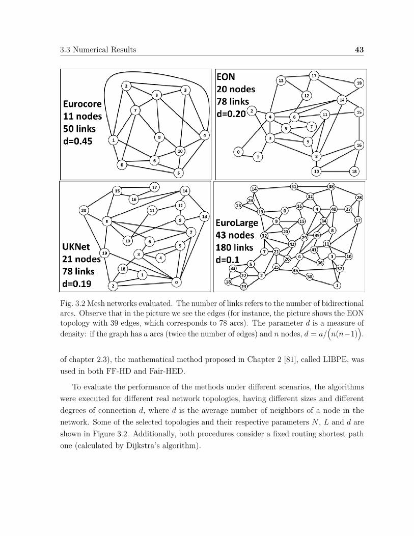
3.3 Numerical Results 43
Fig. 3.2 Mesh networks evaluated. The number of links refers to the number of bidirectionalarcs. Observe that in the picture we see the edges (for instance, the picture shows the EONtopology with 39 edges, which corresponds to 78 arcs). The parameter d is a measure ofdensity: if the graph has a arcs (twice the number of edges) and n nodes, d = a/
(n(n−1)
).
of chapter 2.3), the mathematical method proposed in Chapter 2 [81], called LIBPE, wasused in both FF-HD and Fair-HED.
To evaluate the performance of the methods under different scenarios, the algorithmswere executed for different real network topologies, having different sizes and differentdegrees of connection d, where d is the average number of neighbors of a node in thenetwork. Some of the selected topologies and their respective parameters N , L and d areshown in Figure 3.2. Additionally, both procedures consider a fixed routing shortest pathone (calculated by Dijkstra’s algorithm).
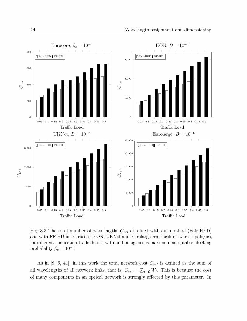
44 Wavelength assignment and dimensioning
0.05 0.1 0.15 0.2 0.25 0.3 0.35 0.4 0.45 0.50
200
400
600
800
Traffic Load
Cne
t
Eurocore, βc = 10−6
Fair-HED FF-HD
0.05 0.1 0.15 0.2 0.25 0.3 0.35 0.4 0.45 0.50
1,000
2,000
3,000
Traffic Load
Cne
t
EON, B = 10−6
Fair-HED FF-HD
0.05 0.1 0.15 0.2 0.25 0.3 0.35 0.4 0.45 0.50
1,000
2,000
3,000
Traffic Load
Cne
t
UKNet, B = 10−6
Fair-HED FF-HD
0.05 0.1 0.15 0.2 0.25 0.3 0.35 0.4 0.45 0.50
5,000
10,000
15,000
20,000
25,000
Traffic Load
Cne
t
Eurolarge, B = 10−6
Fair-HED FF-HD
Fig. 3.3 The total number of wavelengths Cnet obtained with our method (Fair-HED)and with FF-HD on Eurocore, EON, UKNet and Eurolarge real mesh network topologies,for different connection traffic loads, with an homogeneous maximum acceptable blockingprobability βc = 10−6.
As in [9, 5, 41], in this work the total network cost Cnet is defined as the sum ofall wavelengths of all network links, that is, Cnet = ∑
ℓ∈L Wℓ. This is because the costof many components in an optical network is strongly affected by this parameter. In

3.3 Numerical Results 45
0.05 0.1 0.15 0.2 0.25 0.3 0.35 0.4 0.45 0.50
200
400
600
800
Traffic Load
Cne
t
Eurocore, βc = 10−3
Fair-HED FF-HD
0.05 0.1 0.15 0.2 0.25 0.3 0.35 0.4 0.45 0.50
1,000
2,000
3,000
Traffic LoadC
net
EON, B = 10−3
Fair-HED FF-HD
0.05 0.1 0.15 0.2 0.25 0.3 0.35 0.4 0.45 0.50
1,000
2,000
3,000
Traffic Load
Cne
t
UKNet, B = 10−3
Fair-HED FF-HD
0.05 0.1 0.15 0.2 0.25 0.3 0.35 0.4 0.45 0.50
5,000
10,000
15,000
20,000
25,000
Traffic Load
Cne
t
Eurolarge, B = 10−3
Fair-HED FF-HD
Fig. 3.4 The total number of wavelengths Cnet obtained with our method (Fair-HED)and with FF-HD on Eurocore, EON, UKNet and Eurolarge real mesh network topologies,for different connection traffic loads, with an homogeneous maximum acceptable blockingprobability βc = 10−3.
fact, it determines how many infrastructure resources are needed to achieve the networkoperation.

46 Wavelength assignment and dimensioning
On the first set of experiments, we analyze the homogeneous QoS constraint case,which means that every network connection has the same maximum acceptable blockingprobability βc = β. In Figure 3.4 we show the total cost Cnet obtained by the FF-HDand Fair-HED methods for the case when all the connections have the same maximumacceptable blocking probability of 10−6 (βc = 10−6, for all c ∈ X ), as a function of thetraffic load, for different network topologies. Additionally, Figure 3.3 shows the Cnet valuefor the same methods, but considering a threshold of βc = 10−3, for all c ∈ X .
As it can be seen in Figure 3.4, in the case of homogeneous QoS constraints, ourproposal (Fair-HED) performs clearly better. In fact, for all the scenarios evaluated inour experiments, the method proposed here requires in general 25% less wavelengths (forϱ = 0.3 which is a representative network load [28]) than the cost of the FF-HD method,considering a threshold of βc = 10−6. In the case of a maximum blocking probability equalto 10−3 (Figure 3.3), the Fair-HED method also significantly outperforms the FF-HDtechnique. In this last case, the Fair-HED method requires in the order of 30% lesswavelengths (always for ϱ = 0.3 [28]) than FF-HD. Notice that each scenario presentedhere achieves to connect the same users (connections) with the same QoS requirements(maximum acceptable blocking probability), but our proposal requires less resources thanFF-HD to do so.
3.3.1 Heterogeneous QoS requirements
Now, as mentioned in the introduction of this chapter, different end-to-end quality ofservices per user on WDM optical networks considering multi-class traffic is of paramountimportance [75–77, 84, 79, 80]. Thus, to assess this kind of scenario, we evaluate bothmethods (FF-HD and Fair-HED) considering heterogeneous QoS constraints. This meansthat each connection has a different quality of service requirement, measured by themaximum acceptable blocking probability (βc).
First, let Z be a set containing different values of quality of service constrains. Then,we predefine a set of different possible values to be assigned to βc, and store them in Z(For example: Z = 10−3, 10−4, 10−5, 10−6).
Next, we assign to each network connection c their maximum blocking probability βc.To make this assignment, we define 3 different criteria to set βc from the values storedon Z, in order to obtain heterogeneous QoS constrains.
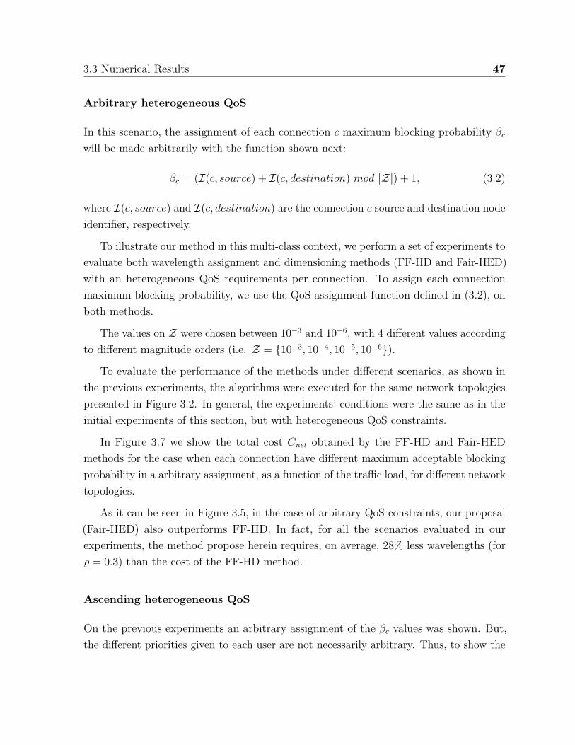
3.3 Numerical Results 47
Arbitrary heterogeneous QoS
In this scenario, the assignment of each connection c maximum blocking probability βc
will be made arbitrarily with the function shown next:
βc = (I(c, source) + I(c, destination) mod |Z|) + 1, (3.2)
where I(c, source) and I(c, destination) are the connection c source and destination nodeidentifier, respectively.
To illustrate our method in this multi-class context, we perform a set of experiments toevaluate both wavelength assignment and dimensioning methods (FF-HD and Fair-HED)with an heterogeneous QoS requirements per connection. To assign each connectionmaximum blocking probability, we use the QoS assignment function defined in (3.2), onboth methods.
The values on Z were chosen between 10−3 and 10−6, with 4 different values accordingto different magnitude orders (i.e. Z = 10−3, 10−4, 10−5, 10−6).
To evaluate the performance of the methods under different scenarios, as shown inthe previous experiments, the algorithms were executed for the same network topologiespresented in Figure 3.2. In general, the experiments’ conditions were the same as in theinitial experiments of this section, but with heterogeneous QoS constraints.
In Figure 3.7 we show the total cost Cnet obtained by the FF-HD and Fair-HEDmethods for the case when each connection have different maximum acceptable blockingprobability in a arbitrary assignment, as a function of the traffic load, for different networktopologies.
As it can be seen in Figure 3.5, in the case of arbitrary QoS constraints, our proposal(Fair-HED) also outperforms FF-HD. In fact, for all the scenarios evaluated in ourexperiments, the method propose herein requires, on average, 28% less wavelengths (forϱ = 0.3) than the cost of the FF-HD method.
Ascending heterogeneous QoS
On the previous experiments an arbitrary assignment of the βc values was shown. But,the different priorities given to each user are not necessarily arbitrary. Thus, to show the

48 Wavelength assignment and dimensioning
0.05 0.1 0.15 0.2 0.25 0.3 0.35 0.4 0.45 0.50
200
400
600
800
Traffic Load
Cne
t
Eurocore, Non-concurrent arbitrary βc
Fair-HED FF-HD
0.05 0.1 0.15 0.2 0.25 0.3 0.35 0.4 0.45 0.50
1,000
2,000
3,000
Traffic LoadC
net
EON, Non-concurrent arbitrary βc
Fair-HED FF-HD
0.05 0.1 0.15 0.2 0.25 0.3 0.35 0.4 0.45 0.50
1,000
2,000
3,000
Traffic Load
Cne
t
UKNet, Non-concurrent arbitrary βc
Fair-HED FF-HD
0.05 0.1 0.15 0.2 0.25 0.3 0.35 0.4 0.45 0.50
5,000
10,000
15,000
20,000
25,000
Traffic Load
Cne
t
Eurolarge, Non-concurrent arbitrary βc
Fair-HED FF-HD
Fig. 3.5 The total number of wavelengths Cnet obtained with our method (Fair-HED) andwith FF-HD on Eurocore, EON, UKNet and Eurolarge real mesh network topologies, fordifferent connection traffic loads, with an heterogeneous maximum acceptable blockingprobability βc. The values of βc are chosen between 10−6 and 10−3 in an arbitrary form.
robustness of our method, we present a different set of experiments using a non-arbitrarycriteria to set each βc heterogeneously.

3.3 Numerical Results 49
The value of each connection βc is assigned according to each connection route length(measured by its number of hops). In this case, the value assigned to βc increases withthe connection c route length.
To this end, we classify each connection c ∈ X depending on its length in number ofhops (i.e. |rc|). Thus, the connections with the same length will be stored on Xh, whereh = |rc|. Let H be the length of the longest connection route on the network. This meansthat we have H sets of connections Xh. This procedure, allows us to define the same QoSrequirement, given by βh, for each connection in Xh. This means βc = βh, when c ∈ Xh.
The values on set Z are ordered from easier to harder to satisfy (e.g. a QoS constraintof 10−3 is easier to fulfill than 10−6, so it will go first).
It remains to choose the values of each βh, with h = 1, 2, ..., H. The idea is to assigna value within the elements on the set Z, to each βh. To this purpose, we classify the H
sets of connection Xh in |Z| categories. These categories are going to be chosen accordingto the connections length h. Thus we assign to βh, with h = 1, 2, ..., H, the z-th valueon Z (with 1 ≤ z ≤ |Z|), if the route lengths h are in the range [1 + (z − 1) · T, 1 + z · T [.The parameter T is:
T = H − 1|Z|
. (3.3)
This method assigns to each connection c in X a maximum blocking probability accordingto the connection length in an ascending order, thus, the longer the connections thestricter the QoS requirements.
We called this procedure “AQOSassignment”.
In algorithmic form the procedure is presented in 3.6.
As presented in the previous scenarios, we perform the same set of experiments toevaluate both wavelength assignment and dimensioning methods (FF-HD and Fair-HED)using the same network topologies. To assign each βc value, we use the QoS assignmentprocedure given in 3.6, on both methods. Figure 3.7 presents the total cost Cnet obtainedby the FF-HD and Fair-HED methods.
The values stored in Z were defined from easier to stricter to fulfill, between 10−3
and 10−6, thus Z = 10−3, 10−4, 10−5, 10−6.
Once again, our proposal (Fair-HED) obtains much better results than FF-HD, usingon average 30% less wavelengths (for ϱ = 0.3) than needed by the FF-HD method.

50 Wavelength assignment and dimensioning
function AQOSassignment// --- input: the graph G (the network), the connections// and the different bounds on the blocking probabilities in Z// ordered from easier to harder to satisfy,// all seen as global variables,// and the set R of predefined routes// --- output: the values of βc per connection
// --- obtain the longest route, and create H sets of connections.1 H=longest(R);2 for h = 1, ..., H3 Xh := φ;
// --- store each connection on their respective Xh set.4 for all connection c5 if (c = h)6 Xh := Xh ∪ c;
// --- evaluate the threshold to make the QoS assignment.7 T = H−1
|Z|
// --- sets βc to each connection following the ascending criteria.8 for h = 1, ..., H9 for z = 0, ..., |Z| − 110 if (1 + (z − 1) · T ) ≤ h < (1 + z · T )11 βh := Z(z);12 break;13 for connection c ∈ Xh
14 βc := βh;
return (βc, forall c ∈ X )
Fig. 3.6 Decision process to assign the QoS constrains in Z to each connection in Xh,with h = 1, 2, ..., H. The criteria used to make the assignment of the βc correspond to theidea of longer the connections the stricter the QoS requirements (ascending heterogeneousQoS constrains criteria)
Descending heterogeneous QoS
The previous experiments have shown the performance of our method in non-arbitraryQoS constrains. Following the same line of thought, we present a final set of experimentsto prove the robustness of our method, no matter the scenario chosen.

3.3 Numerical Results 51
0.05 0.1 0.15 0.2 0.25 0.3 0.35 0.4 0.45 0.50
200
400
600
800
Traffic Load
Cne
t
Eurocore, Ascending βc
Fair-HED FF-HD
0.05 0.1 0.15 0.2 0.25 0.3 0.35 0.4 0.45 0.50
1,000
2,000
3,000
Traffic LoadC
net
EON, Ascending βc
Fair-HED FF-HD
0.05 0.1 0.15 0.2 0.25 0.3 0.35 0.4 0.45 0.50
1,000
2,000
3,000
Traffic Load
Cne
t
UKNet, Ascending βc
Fair-HED FF-HD
0.05 0.1 0.15 0.2 0.25 0.3 0.35 0.4 0.45 0.50
5,000
10,000
15,000
20,000
25,000
Traffic Load
Cne
t
Eurolarge, Ascending βc
Fair-HED FF-HD
Fig. 3.7 The total number of wavelengths Cnet obtained with our method (Fair-HED) andwith FF-HD on Eurocore, EON, UKNet and Eurolarge real mesh network topologies, fordifferent connection traffic loads, with an heterogeneous maximum acceptable blockingprobability βc. The values of βc are chosen between 10−3 and 10−6 in an ascending order,proportionally to the connections route lengths.
In this case, the value of each βc is also assigned according to the number of hops ofeach connection, but decreasing with the route length. To do this, we follow the same
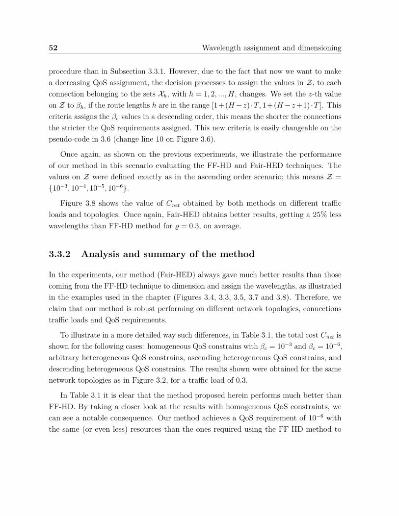
52 Wavelength assignment and dimensioning
procedure than in Subsection 3.3.1. However, due to the fact that now we want to makea decreasing QoS assignment, the decision processes to assign the values in Z, to eachconnection belonging to the sets Xh, with h = 1, 2, ..., H, changes. We set the z-th valueon Z to βh, if the route lengths h are in the range [1+(H−z) ·T, 1+(H−z +1) ·T ]. Thiscriteria assigns the βc values in a descending order, this means the shorter the connectionsthe stricter the QoS requirements assigned. This new criteria is easily changeable on thepseudo-code in 3.6 (change line 10 on Figure 3.6).
Once again, as shown on the previous experiments, we illustrate the performanceof our method in this scenario evaluating the FF-HD and Fair-HED techniques. Thevalues on Z were defined exactly as in the ascending order scenario; this means Z =10−3, 10−4, 10−5, 10−6.
Figure 3.8 shows the value of Cnet obtained by both methods on different trafficloads and topologies. Once again, Fair-HED obtains better results, getting a 25% lesswavelengths than FF-HD method for ϱ = 0.3, on average.
3.3.2 Analysis and summary of the method
In the experiments, our method (Fair-HED) always gave much better results than thosecoming from the FF-HD technique to dimension and assign the wavelengths, as illustratedin the examples used in the chapter (Figures 3.4, 3.3, 3.5, 3.7 and 3.8). Therefore, weclaim that our method is robust performing on different network topologies, connectionstraffic loads and QoS requirements.
To illustrate in a more detailed way such differences, in Table 3.1, the total cost Cnet isshown for the following cases: homogeneous QoS constrains with βc = 10−3 and βc = 10−6,arbitrary heterogeneous QoS constrains, ascending heterogeneous QoS constrains, anddescending heterogeneous QoS constrains. The results shown were obtained for the samenetwork topologies as in Figure 3.2, for a traffic load of 0.3.
In Table 3.1 it is clear that the method proposed herein performs much better thanFF-HD. By taking a closer look at the results with homogeneous QoS constraints, wecan see a notable consequence. Our method achieves a QoS requirement of 10−6 withthe same (or even less) resources than the ones required using the FF-HD method to
3.3 Numerical Results 53
0.05 0.1 0.15 0.2 0.25 0.3 0.35 0.4 0.45 0.50
200
400
600
800
Traffic Load
Cne
t
Eurocore, Descending βc
Fair-HED FF-HD
0.05 0.1 0.15 0.2 0.25 0.3 0.35 0.4 0.45 0.50
1,000
2,000
3,000
Traffic LoadC
net
EON, Descending βc
Fair-HED FF-HD
0.05 0.1 0.15 0.2 0.25 0.3 0.35 0.4 0.45 0.50
1,000
2,000
3,000
Traffic Load
Cne
t
UKNet, Descending βc
Fair-HED FF-HD
0.05 0.1 0.15 0.2 0.25 0.3 0.35 0.4 0.45 0.50
5,000
10,000
15,000
20,000
25,000
Traffic Load
Cne
t
Eurolarge, Descending βc
Fair-HED FF-HD
Fig. 3.8 The total number of wavelengths Cnet obtained with our method (Fair-HED) andwith FF-HD on Eurocore, EON, UKNet and Eurolarge real mesh network topologies, fordifferent connection traffic loads, with an heterogeneous maximum acceptable blockingprobability βc. The values of βc are chosen between 10−6 and 10−3 in an descending order,proportionally to the connections route lengths.
satisfy a βc value equal to 10−3. This clearly illustrate that the FF-HD over-dimensionsthe network links.

54 Wavelength assignment and dimensioning
It is also interesting to analyze the results obtained with Heterogeneous QoS re-quirements. By considering the ascending QoS constraints scenario, the FF-HD methodrequires basically the same amount of wavelengths than considering an homogeneousQoS equal to 10−6. This comparison verifies that the FF-HD dimensioning is stronglyinfluenced by the worst case scenario, because of the stricter blocking probability require-ment. This situation makes the FF-HD method assign more wavelengths than neededto the connections with lower QoS requirement levels. This situation is not observed onthe Fair-HED method, since the number of wavelengths in the case of homogeneous QoSrequirements is higher than any heterogeneous QoS constraints (ascending and descendingscenarios), thus providing a closer gap between the QoS required and the actual QoSoffered to each network connection. The latter shows how important is to consider thedifferent QoS requirements in the wavelength assignment and dimensioning problem onmulti-class optical networks.
In addition, the results shown by the heterogeneous ascending and decreasing QoSrequirements are clearly different. On the first hand, the ascending QoS scenario canbe considered as a worst case, where the longer routes require a tough QoS demand tosatisfy. On the other hand, the descending QoS scenario can be reckon as a best case one,where the longer the route, the looser the QoS demand. First, no matter the scenarioour method performs better than the commonly used FF-HD. Second, this examplesshows that the definition of multiple classes of services affect the network performance.Therefore, this examples provide an insight on how we can take advantage of the classes ofuser to have more efficient networks. For instance, by defining a policy as the descendingheterogeneous QoS constraints requires less network resources than an any other QoSassignment criteria presented on this work.
Let us discuss here some qualitative reasons that justify the better results of Fair-HEDover FF-HD:
• Our method assigns a different number of wavelengths to each network link (thisis called Heterogeneous Dimensioning), such that the blocking probability of eachconnection does not exceed a predefined maximum blocking probability. This takesadvantage of the fact that real networks are hardly symmetric, making difficult tobalance the traffic loads offered to the different links. Therefore, each network linkcapacity can be dimensioned differently, since they have a different amount of usersassigned to.

3.4 Conclusions 55
• Our technique proposes a new wavelength assignment policy called “Fairness Policy”.This policy consists of providing to each network user a quality of service (blockingprobability) as close as possible to the one required in the SLA, since each user mayhave different quality of service requirements. This way the method diminishes thewavelength dimensioning since each connection uses only the wavelengths neededto satisfy their QoS demand.
• The usual blocking probability evaluation technology is based on simulation, whichis a slow procedure. Consequently, the evaluation process is limited to only afew restricted scenarios. So, to find the best possible solution, researchers applysome criteria to restrict the solutions search (heuristics), for example, makingchoices as homogeneous wavelength dimensioning and using plain first-fit wavelengthassignment. The method we proposed is able to outperform these methodologies,so we can conclude that such heuristic solutions are not using good assumptionsand taking appropiate decisions.
• Our method can solve the problem of wavelength assignment and dimensioningusing any method available to evaluate the connection’s blocking probability. Forinstance, it can rely on simulation or on any analytical method from the literature.Thus, the time require to solve both problems strongly depends on the chosenmethod to evaluate the QoS, since it requires several evaluations of the connectionsblocking probability. At this point, we suggest using the fast, simple and veryaccurate method proposed in Chapter 2, which allows to dimension the network ina very short time (less than a second, say).
3.4 Conclusions
This chapter presents a novel method to jointly calculate the number of wavelengthsneeded on each network link, and to define a strategy to approach the wavelengthassignment procedure during the network operation based on the well known First-fitscheme, in Dynamic WDM Optical Networks without wavelength conversion. This jointsolution allows us to obtain a global solution to these problems, which in general is betterthan to obtain them separately.
56 Wavelength assignment and dimensioning
The methodology differs considerably from those published so far. It assigns a differentnumber of wavelengths to each network link, so that the blocking probability of each useris lower than a certain pre-specified threshold (which is a design parameter of the network).Additionally, the technique proposes a fair wavelength assignment policy, offering to eachnetwork user a quality of service as close as possible to the one defined in the SLA, sinceeach user may have different quality of service requirements (multi-class networks).
Our proposal relies on the blocking probability method proposed in Chapter 2, thusit requires less than a second to solve both problems. Nevertheless, observe that it canbe used calling any other procedure to evaluate the blocking probability (e.g. by meansof simulation or another method available). This means that the time required to solvethe wavelength assignment and dimensioning strongly depends on the method used tocalculate this blocking probability.

3.4 Conclusions 57
Para
met
ers
Hom
ogen
eous
βc
=10
−3
Hom
ogen
eous
βc
=10
−6
Arb
itrar
yH
eter
ogen
eous
βc
Asc
endi
ngH
eter
ogen
eous
βc
Des
cend
ing
Het
erog
eneo
usβ
c
Top o
logy
Fair-
HED
FF-H
DFa
ir-H
EDFF
-HD
Fair-
HED
FF-H
DFa
ir-H
EDFF
-HD
Fair-
HED
FF-H
D
Euro
core
297
400
395
500
358
500
368
500
336
450
EON
1251
1872
1567
2184
1448
2106
1496
2184
1356
1950
UK
Net
1419
1950
1771
2262
1646
2262
1699
2262
1519
1950
Euro
larg
e91
7512
420
1047
413
680
9987
1332
010
075
1350
097
8712
600
Tabl
e3.
1To
taln
umbe
rof
wave
leng
ths
requ
ired
byth
eFa
ir-H
EDan
dFF
-HD
met
hods
with
:ho
mog
eneo
usQ
oSco
nstr
ains
(Hom
ogen
eous
βc
=10
−3
and
βc
=10
−6 )
,no
n-co
ncur
rent
arbi
trar
yhe
tero
gene
ous
QoS
cons
trai
ns(A
rbitr
ary
Het
erog
eneo
usβ
c),
asce
ndin
ghe
tero
gene
ous
QoS
cons
trai
ns(A
scen
ding
Het
erog
eneo
usβ
c),
and
desc
endi
nghe
tero
gene
ous
QoS
cons
trai
ns(D
esce
ndin
gH
eter
ogen
eous
βc),
for
Euro
core
,EO
N,U
KN
etan
dEu
rola
rge
netw
ork
topo
logi
es,c
onsid
erin
ga
conn
ectio
nm
ean
traffi
clo
adof
0.3.


Chapter 4
Routing, Wavelength Assignmentand Dimensioning
4.1 Introduction
“Routing” is a basic component of the network operation: every connection is definedby a pair of nodes in the network, the source and the destination, and for each pair,the designer must assign a route to be followed by the data to be transmitted. Then,the routing problem consist in to assign to each connection a specific route. To solvethe routing problem, various approaches has been proposed, Zang et al. [10] provides acomprehensive survey on these routing algorithms, which are summarized next:
• Fixed Routing: Considered as the most straightforward approach, this schemealways assigns to each user the same fixed route to connect from the source todestination. This route is defined previous to the network operation and it does notchange over time. Shortest Path—First Fit (SP-FF) [16, 85, 9, 86, 12, 11] is themost common fixed routing approach. SP-FF has shown to be the fastest algorithmavailable to date, since it uses pre-established routes and the a simple wavelengthallocation algorithm (Fist-fit). Be that as it may, it has been known to have, ingeneral, a higher blocking probability than the next 2 approaches, due the lack ofalternative paths to connect any source-destination pair of nodes in case of blocking.

60 Routing, Wavelength Assignment and Dimensioning
• Fixed-Alternate Routing: This approach assigns to each network user a set ofalternative paths (more than one) to offer a connection from source to destinationnode [10, 85, 9, 12, 11]. This paths are typically disjoint between them (i.e. theydo not share any resources). As fixed routing approach, the paths are store inrouting tables prior the network operation, to be addressed on demand. Thus, tocommunicate the source node to destination, each user attempts to connect bythe first route in the set. If, there is any blocking among the path links, then ittries with the next path until it finds an available path in the set to make thetransmissions or blocked in all of them. K-Alternate Paths using Shortest Path-FirstFit (K-SP-FF) is the most common approach in literature, usually with k=3. Itis known to perform a good compromise between computational complexity andperformance, and it is expected to have a better performance than fixed routingwithout a global knowledge of the network state [12].
• Adaptive Routing: This methodology chooses the route from a source node todestination on demand, depending on the network state, hence it requires a constantknowledge of the network situation [9, 12, 11]. Adaptive Unconstrained Rout-ing—Exhaustive (AUR-E) as shown to be the best adaptive routing method [6].This approach has shown to have the lowest blocking probability to date due tothe online execution of Dijkstra algorithm per transmission request [10]. In fact, ithas been reported that AUR-E requires on average a 15% less wavelengths than3-SP-FF to achieve the same blocking probability requirements [5]. Nevertheless,this operation scheme performs a huge overhead on the network, thus a slow networkoperation [8].
Among the different routing algorithms proposed to date, fixed routing is the moststudied and typically used for real world networks [87, 26, 27, 25, 85, 88, 5, 9, 86, 11].
The Wavelength dimensioning (WD) problem, as explain on chapter 3, determineshow many wavelengths should be assigned to each link of the network in order to achieve acompromise between efficiency and the network infrastructure cost. The usual procedureto solve the WD problem has been to assign the same number of wavelengths to eachnetwork link (called Homogeneous Dimensioning). This procedure has been generallysolved by means of simulation, thus it does not allow to explore every possible solutiondue the time-consuming task involved.

4.1 Introduction 61
The Wavelength assignment (WA) problem asses the problem to chose which wave-length is going to be used by each users, taking into account the wavelength continuityrestrain on networks without wavelength conversion. First-fit has been the most com-mon and fastest method used to date, and is preferred in practice because of its smallcomputational overhead and low complexity.
These problems are solved while aiming to simultaneously minimize the networkcost, while guaranteeing that the network performance meets the level established in theService Level Agreement (SLA). Then, We call these problems together as the Routing,and Wavelength Assignment and dimensioning (R&WAD) problem.
This problem has been extensively studied on the literature, because of their greatimpact on network cost (CapEx) and on network performance. These tasks are usuallysolved separately [10, 11]. This happens due to the fact that solving them simultaneouslyhave a great complexity associated. Then, to diminish this constrain, a traditional solutionhas been as follows: first the routes are calculated; later, the wavelength assignment ischosen and the number of wavelengths for each network link are dimension accordingly,while satisfying some pre-established performance restrictions.
By solving separately the Routing, the Wavelength Assignment and the WavelengthDimensioning, is possible to achieve good local solutions to both problems. Since thewavelength dimensioning has been usually solved by simulation, the time-consumingtask involved does not allowed to explore every possible solution, requiring to divide theR&WD problem. However, the approach misses the opportunity to find a good globalsolution found when solving them simultaneously. One way to overcome this problem is tosolve the dimensioning by using heuristics, but they should be validated extensively, as wedid on chapter 3 proposal. Recently in [41], an exhaustively validated heuristic strategy,called CPR (Cheapest Path Routing) was applied, solving both routing and wavelengthdimensioning jointly, in the context of WDM optical networks with wavelength conversioncapabilities. Its performance was better than local strategies approaches.
In this chapter we propose a novel procedure to simultaneously solve the routing,wavelength assignment and wavelength dimensioning (which we call the Cheapest Pathby Layers CPL method). The method assigns to each source-destination pair of nodes thecheapest route while attempting to balance the traffic load offer to each link. The methodalso evaluates the number of wavelengths Wℓ for each link ℓ of the network, ensuring
62 Routing, Wavelength Assignment and Dimensioning
that the blocking probability of any connection request will be lower than the predefinedthreshold llβc. The method relies on a wavelength assignment and dimensioning completelydifferent than the ones proposed to date. It introduces 2 new characteristics: the numberof wavelengths (in general) are different on each link (heterogeneous dimensioning), whilesatisfying a predefined quality of service threshold; and the wavelength assignment usedintroduces a Fairness Policy to each network user providing a quality of service as closeas possible as the one defined on the SLA.
The remainder of this paper is as follows: Section 4.2 presents the new algorithm.Section 4.3 contains some results obtained by the proposed algorithm, which are comparedwith those obtained with the current best methods in a set of different scenarios. Finally,the conclusions of the study are given in Section 4.4.
4.2 Routing and Wavelength Dimensioning Strategy
This section contains the main contribution of the paper. We present first the modelused and the related assumptions. Then, we describe the main sub-procedures necessaryto our technique. Last, we present the algorithm.
4.2.1 Model and assumptions
We define the same model and assumptions than previous chapters. Thus, if you arealready familiar with it, you are welcome to skip this subsection (continue in 4.2.2).
The network topology is represented by a graph G = (N ,L), where N is the set ofnetwork nodes or vertices and L is the set of unidirectional links (the arcs in G), withrespective cardinalities |N | = N and |L| = L. The set of connections X ⊆ N 2, withcardinality |X | = X, is composed by all the source-destination pairs with communicationbetween them, also called “users” in the text.
To represent the traffic between a given source-destination pair, an ON-OFF model isused. Consider connection c. During any of its ON periods, whose average length is tON c,the source transmits at a constant rate (which is the rate associated to the wavelength).During an OFF period, with average length tOFF c, the source refrains from transmittingdata.

4.2 Routing and Wavelength Dimensioning 63
To simplify the presentation, the constant transmission rate during the ON periods isdetermined by the used technology, that will be our rate unity. Consequently, the trafficload of connection c, denoted by ϱc, is given by the following expression:
ϱc = tON c
tON c + tOFF c
. (4.1)
Observe that we address here the general case where the load can be different for eachconnection, the so-called heterogeneous situation, instead of the usual homogeneous casewhere the load is assumed to be the same for all users.
Let R = rc | c ∈ X be the set of routes that enable communications among thedifferent users, where rc is the route associated with connection c ∈ X . The set R isalso denominated set of primary routes, because this set alone does not offer any faulttolerance to the possible failure of network links.
LetW = Wℓ | ℓ ∈ L be the set containing the number of wavelengths associated withthe unidirectional network links, where Wℓ, ℓ ∈ L, is the number of wavelengths on link ℓ.The value Wℓ, for every ℓ ∈ L, will be evaluated so that the blocking probability BPc, ofeach connection c ∈ X be less than or equal to a given pre-specified threshold βc and thetotal number of available network wavelengths be as small as possible. Remark that thepre-defined threshold value βc can be different for each network connection, allowing themethod to solve these problems when there are classes of users with different priorities.
As in [5, 9, 41], in this work the total network cost Cnet is defined as the sum of allwavelengths of all network links, that is, Cnet = ∑
ℓ∈L Wℓ.
4.2.2 Sub-procedures needed by our CPL method
The method needs a few sub-procedures to work. They are described now. Since thegiven graph and the set of connections (or users) are fixed data that never change, aswell as the upper bounds βc of the blocking connection probabilities, we will omit themin the list of the parameters of the procedures. Also, when we refer to the network cost,we will write simply Cnet because we must in general change many times during thecomputational process the capacities of the links.

64 Routing, Wavelength Assignment and Dimensioning
InitialRoutes(): initial computation of the shortest routes Our method starts bycomputing an initial set of routes. For each connection (s, t) we look for the shortestroute from s to t in the graph, implicitly assuming that the capacity of all involved links(that is, the number of wavelengths available at each arc of the graph) is infinite. Let ussymbolically write R := InitialRoutes() to represent the execution of this sub-procedure.
CandidateRoutes(δ, c): evaluation of δ shortest routes Our procedure requires tocompute an initial set of routes to each connection c ∈ X . This routes will be consideredas candidates to be use as the definitive route. This can be done by any availabletechnique (e.g. Yen’s algorithm [89]). The number of routes in the set is defined by theparameter δ. Then, for each connection c we look for a set of δ shortest routes fromsource to destination in the graph G, denoted as Hc, again assuming that the capacity ofall involved links is infinite. Let us algorithmically write Hc := CandidateRoutes(δ, c)to represent the evaluation of this sub-procedure.
BestOf (): given the possible routes provided by function CandidateRoutes(δ, c),find the best of them The idea is to choose which one of the routes defined bythe function CandidateRoutes(δ, c) stored on Hc, has the smallest cost (given by routesassigned at the moment, considering each connection traffic load), that is, the sum of allthe link ℓ relative costs Cℓ. The route cost is denoted as σ(i), as the i-th route cost in Hc,updated on the procedure. The one with the smallest cost is called the “best” of themall, storing it on rc. Symbolically, we write rc := BestOf (Hc).
WavelengthAD(): given the routes and the thresholds βc, compute the capacitiesand the wavelength assignment policy We call WavelengthAD this sub-procedure.The problem consists in finding, for each link ℓ ∈ L, a capacity Wℓ such that the end-to-end blocking probability BPc of every user c ∈ X passing through the link ℓ is less thanthe given threshold or upper bound, denoted as βc, while choosing which wavelength isgoing to be used by each connection. The routes R are considered fixed and calculatedbefore the evaluation of this sub-procedure.
The wavelength assignment method is based on the First-Fit method, due it is thefastest and simplest method with a good performance in terms of blocking probability,
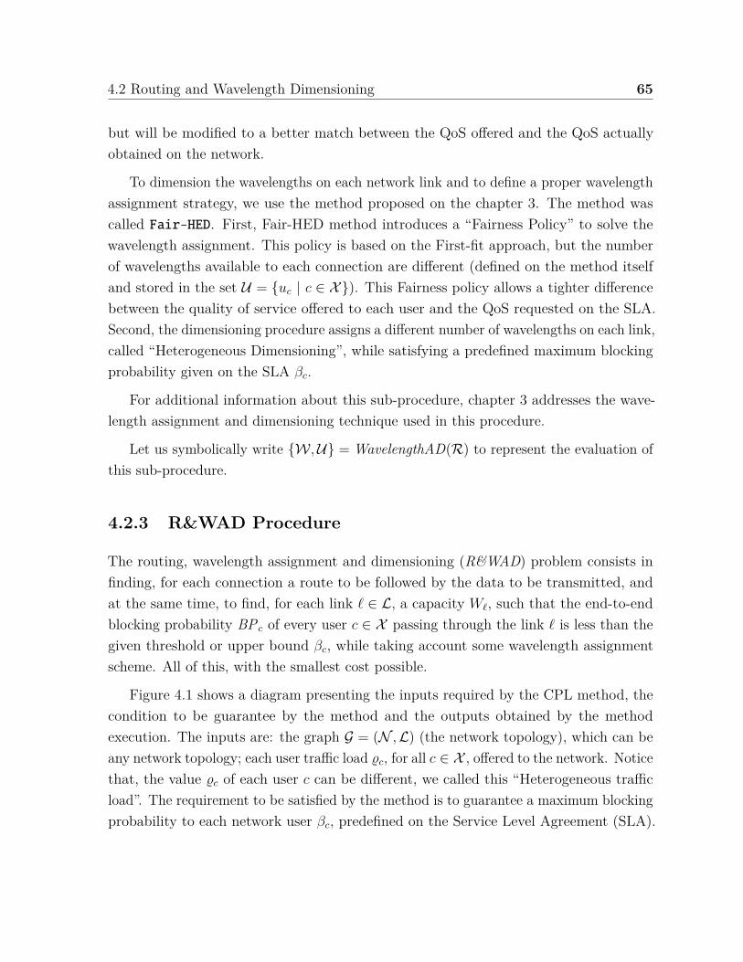
4.2 Routing and Wavelength Dimensioning 65
but will be modified to a better match between the QoS offered and the QoS actuallyobtained on the network.
To dimension the wavelengths on each network link and to define a proper wavelengthassignment strategy, we use the method proposed on the chapter 3. The method wascalled Fair-HED. First, Fair-HED method introduces a “Fairness Policy” to solve thewavelength assignment. This policy is based on the First-fit approach, but the numberof wavelengths available to each connection are different (defined on the method itselfand stored in the set U = uc | c ∈ X). This Fairness policy allows a tighter differencebetween the quality of service offered to each user and the QoS requested on the SLA.Second, the dimensioning procedure assigns a different number of wavelengths on each link,called “Heterogeneous Dimensioning”, while satisfying a predefined maximum blockingprobability given on the SLA βc.
For additional information about this sub-procedure, chapter 3 addresses the wave-length assignment and dimensioning technique used in this procedure.
Let us symbolically write W ,U = WavelengthAD(R) to represent the evaluation ofthis sub-procedure.
4.2.3 R&WAD Procedure
The routing, wavelength assignment and dimensioning (R&WAD) problem consists infinding, for each connection a route to be followed by the data to be transmitted, andat the same time, to find, for each link ℓ ∈ L, a capacity Wℓ, such that the end-to-endblocking probability BPc of every user c ∈ X passing through the link ℓ is less than thegiven threshold or upper bound βc, while taking account some wavelength assignmentscheme. All of this, with the smallest cost possible.
Figure 4.1 shows a diagram presenting the inputs required by the CPL method, thecondition to be guarantee by the method and the outputs obtained by the methodexecution. The inputs are: the graph G = (N ,L) (the network topology), which can beany network topology; each user traffic load ϱc, for all c ∈ X , offered to the network. Noticethat, the value ϱc of each user c can be different, we called this “Heterogeneous trafficload”. The requirement to be satisfied by the method is to guarantee a maximum blockingprobability to each network user βc, predefined on the Service Level Agreement (SLA).

66 Routing, Wavelength Assignment and Dimensioning
Fig. 4.1 Diagram showing the inputs required to run the CPL method, the conditionto be guarantee by the method, and the outputs delivered by the method, to solve therouting and wavelength dimensioning problem.
Finally, the method’s outputs are the set of routes R allowing to provide communicationto each network connection c, for all c ∈ X , and the amount of wavelength Wℓ necessaryon each network link ℓ, for all ℓ ∈ L.
Let the wavelengths be numbered sequentially (i.e. 1, 2, . . . Wℓ).
As mentioned on the dimensioning sub-procedure the method uses a First-Fit wave-length assignment approach, and during the method’s execution, the fairness policy isobtained to complete the wavelength assignment strategy.
It remains to specify the procedure used to compute the connection blocking proba-bilities, necessary to evaluate the quality of service offered to each connection c. For thispurpose, we use the method proposed in the previous chapter 2 [81], a fast and simplenumerical evaluation considering heterogeneous traffic loads on each network connectionon optical networks with wavelength continuity constrains.
In algorithmic form, the procedure can be written as shown in Figure 4.2.
Symbolically, the execution of the whole routing and wavelength dimensioning proce-dure will be written R,W := CPL(), since its output is the set of wavelengths and theset of all the connections route.
First, we compute a set of candidate paths to each connection c ∈ X (see line 1 to 4).This paths are candidates to be the final connection route. The amount of routes is set

4.2 Routing and Wavelength Dimensioning 67
function CPL()// --- input: the graph (the network), the connections// and the bounds on the blocking probabilities βc,// all seen as global variables// --- output: the routes R and the wavelengths per link W.
// --- calculate the set of candidate paths1 R ′ := InitialRoutes(); // shortest paths2 for all connection c3 δ := Length(R ′); // shortest route length4 Hc := CandidateRoutes(δ, c);
// --- start computing connections path and set them operational5 X := Sort(X ,R ′) // sort connections by route’s length6 P := φ; // no operational connections7 c := 0;
// --- define 1 hop length connections path8 while connection c length equals to 19 rc := Hc(0) // set the only possible route10 P := P ∪ c; // connection c is operational11 c++;
// --- compute next connections, choosing the best path in Hc
12 do13 for i := 1 to Length(Hc)14 ϱℓ :=
∑c∈X \XF ∧ℓ∈rc
ϱc; // operational + candidate route
15 ϱ :=∑
ℓ∈L ϱℓ
L ;16 Cℓ := eϱℓ−ϱ;17 σ(i) := ∑ℓ∈rc
Cℓ; // i-th path cost18 rc := BestOf (Hc); // the best route is chosen19 P := P ∪ c; // connection c is operational20 c++;21 until (P ≡ X )22 W := WavelengthAD(R); // --- with W, QoS is satisfied23 Cnet := Cost(W); // --- Cnet = W1 + · · ·+ WL
24 return (R,W)
Fig. 4.2 function CPL() proposed on this thesis chapter to solve the R&WAD problem,denoted as “Cheapest Path By Layers”.
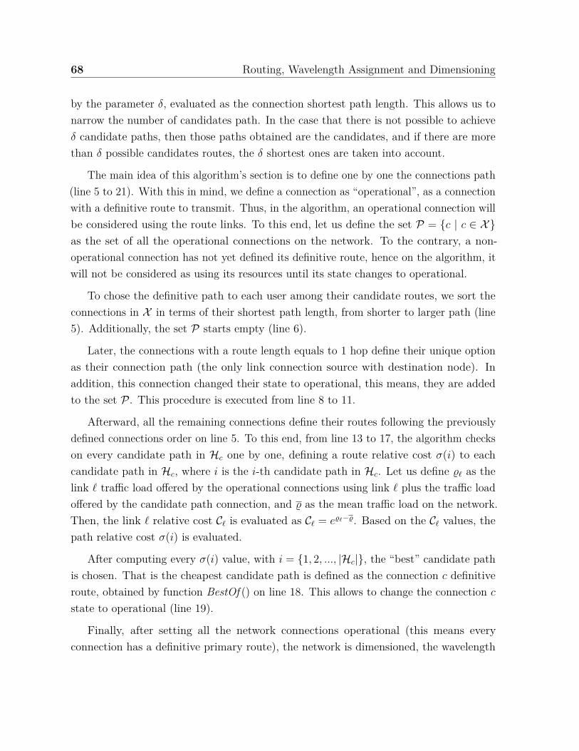
68 Routing, Wavelength Assignment and Dimensioning
by the parameter δ, evaluated as the connection shortest path length. This allows us tonarrow the number of candidates path. In the case that there is not possible to achieveδ candidate paths, then those paths obtained are the candidates, and if there are morethan δ possible candidates routes, the δ shortest ones are taken into account.
The main idea of this algorithm’s section is to define one by one the connections path(line 5 to 21). With this in mind, we define a connection as “operational”, as a connectionwith a definitive route to transmit. Thus, in the algorithm, an operational connection willbe considered using the route links. To this end, let us define the set P = c | c ∈ Xas the set of all the operational connections on the network. To the contrary, a non-operational connection has not yet defined its definitive route, hence on the algorithm, itwill not be considered as using its resources until its state changes to operational.
To chose the definitive path to each user among their candidate routes, we sort theconnections in X in terms of their shortest path length, from shorter to larger path (line5). Additionally, the set P starts empty (line 6).
Later, the connections with a route length equals to 1 hop define their unique optionas their connection path (the only link connection source with destination node). Inaddition, this connection changed their state to operational, this means, they are addedto the set P . This procedure is executed from line 8 to 11.
Afterward, all the remaining connections define their routes following the previouslydefined connections order on line 5. To this end, from line 13 to 17, the algorithm checkson every candidate path in Hc one by one, defining a route relative cost σ(i) to eachcandidate path in Hc, where i is the i-th candidate path in Hc. Let us define ϱℓ as thelink ℓ traffic load offered by the operational connections using link ℓ plus the traffic loadoffered by the candidate path connection, and ϱ as the mean traffic load on the network.Then, the link ℓ relative cost Cℓ is evaluated as Cℓ = eϱℓ−ϱ. Based on the Cℓ values, thepath relative cost σ(i) is evaluated.
After computing every σ(i) value, with i = 1, 2, ..., |Hc|, the “best” candidate pathis chosen. That is the cheapest candidate path is defined as the connection c definitiveroute, obtained by function BestOf () on line 18. This allows to change the connection c
state to operational (line 19).
Finally, after setting all the network connections operational (this means everyconnection has a definitive primary route), the network is dimensioned, the wavelength
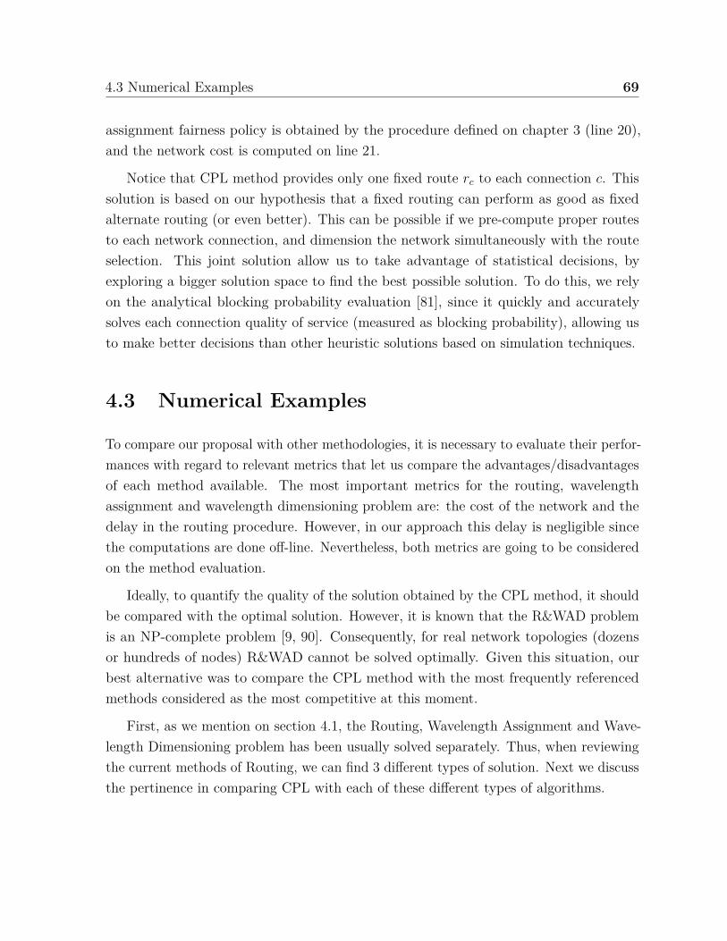
4.3 Numerical Examples 69
assignment fairness policy is obtained by the procedure defined on chapter 3 (line 20),and the network cost is computed on line 21.
Notice that CPL method provides only one fixed route rc to each connection c. Thissolution is based on our hypothesis that a fixed routing can perform as good as fixedalternate routing (or even better). This can be possible if we pre-compute proper routesto each network connection, and dimension the network simultaneously with the routeselection. This joint solution allow us to take advantage of statistical decisions, byexploring a bigger solution space to find the best possible solution. To do this, we relyon the analytical blocking probability evaluation [81], since it quickly and accuratelysolves each connection quality of service (measured as blocking probability), allowing usto make better decisions than other heuristic solutions based on simulation techniques.
4.3 Numerical Examples
To compare our proposal with other methodologies, it is necessary to evaluate their perfor-mances with regard to relevant metrics that let us compare the advantages/disadvantagesof each method available. The most important metrics for the routing, wavelengthassignment and wavelength dimensioning problem are: the cost of the network and thedelay in the routing procedure. However, in our approach this delay is negligible sincethe computations are done off-line. Nevertheless, both metrics are going to be consideredon the method evaluation.
Ideally, to quantify the quality of the solution obtained by the CPL method, it shouldbe compared with the optimal solution. However, it is known that the R&WAD problemis an NP-complete problem [9, 90]. Consequently, for real network topologies (dozensor hundreds of nodes) R&WAD cannot be solved optimally. Given this situation, ourbest alternative was to compare the CPL method with the most frequently referencedmethods considered as the most competitive at this moment.
First, as we mention on section 4.1, the Routing, Wavelength Assignment and Wave-length Dimensioning problem has been usually solved separately. Thus, when reviewingthe current methods of Routing, we can find 3 different types of solution. Next we discussthe pertinence in comparing CPL with each of these different types of algorithms.

70 Routing, Wavelength Assignment and Dimensioning
Fixed routing : This strategy provides connectivity to each user with only one route,computed before the network operations and stored on routing tables. Thus, each useruses the same path every time he attempts to transmit, even if their links path are alreadycongested (causing a blocking situation). Among this strategy solutions, SP-FF (ShortestPath - First Fit) is the algorithm most commonly referenced today. It has shown to bethe simplest and fastest algorithm to date with a very good performance measured asblocking probability.
Fixed alternate routing : This strategy computes a set of disjoint routes to alloweach user to transmit. It is similar to fixed routing in the sense it calculates the routesset previous the network operation, but during the network operation it provides severalalternatives to achieve communication between the source and destination node. Thispaths are stored on routing tables (as the fixed routing approach). The standard mostreferenced algorithm, and considered the best so far is the K-SP-FF (K-Shortest Path-First Fit), due to the fact it has a good compromise between operation complexity andperformance, and it performs better than SP-FF.
Adaptive routing : This method computes each user path on demand, this means,each time a user attempts to transmit on the network. Adaptive Unconstrained Rout-ing—Exhaustive (AUR-E) is known to be the best adaptive routing method. As previouslymentioned, this strategy usually has a lower blocking probability than the previous ap-proaches, but it causes a huge overhead on the network since it requires to execute therouting algorithm per request. Evidently, this on-line strategy causes a slow re-routing.Then, this type of method does not represent a practical mechanism to solve the routingproblem. Therefore, the AUR-E method was not considered for comparison with themethod proposed in this chapter.
Consequently, SP-FF and K-SP-FF methods are the most appropriate routing methodto be compared with our algorithm. For instance, the value of K on the K-SP-FF techniquewas chosen equal to 3, since a higher number does not achieves a better performance interms of wavelength requirements [5].
With regard to the dimensioning problem, as mentioned on the wavelength dimension-ing chapter (Ch.3) the Homogeneous Wavelength Dimensioning has proven to be the most

4.3 Numerical Examples 71
Fig. 4.3 Mesh networks evaluated. The number of links refers to the number of bidirectionalarcs. Observe that in the picture we see the edges (for instance, the picture shows theEurocore topology with 25 edges, which corresponds to 50 arcs). The parameter dis a measure of density: if the graph has a arcs (twice the number of edges) and n
nodes, d = a/(n(n− 1)
).
frequently used and referenced, thus this method will be used to solve the dimensioningproblem.
Accordingly, SP-FF and K-SP-FF routing methods with an Homogeneous wavelengthdimensioning are the most suitable R&WD methods to compare with.
One of the main objectives of the R&WAD method is to satisfy the quality of servicerequirements of each user, predefined on the SLA. Then CPL, SP-FF and K-SP-FFmethods are going to be computed in order to guarantee a maximum connection blockingprobability. Thus, to evaluate the corresponding blocking probabilities, the mathematical
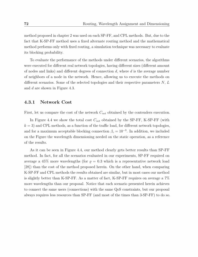
72 Routing, Wavelength Assignment and Dimensioning
method proposed in chapter 2 was used on each SP-FF, and CPL methods. But, due to thefact that K-SP-FF method uses a fixed alternate routing method and the mathematicalmethod performs only with fixed routing, a simulation technique was necessary to evaluateits blocking probability.
To evaluate the performance of the methods under different scenarios, the algorithmswere executed for different real network topologies, having different sizes (different amountof nodes and links) and different degrees of connection d, where d is the average numberof neighbors of a node in the network. Hence, allowing us to execute the methods ondifferent scenarios. Some of the selected topologies and their respective parameters N , L
and d are shown in Figure 4.3.
4.3.1 Network Cost
First, let us compare the cost of the network Cnet obtained by the contenders execution.
In Figure 4.4 we show the total cost Cnet obtained by the SP-FF, K-SP-FF (withk = 3) and CPL methods, as a function of the traffic load, for different network topologies,and for a maximum acceptable blocking connection βc = 10−3. In addition, we includedon the Figure the wavelength dimensioning needed on the static operation, as a referenceof the results.
As it can be seen in Figure 4.4, our method clearly gets better results than SP-FFmethod. In fact, for all the scenarios evaluated in our experiments, SP-FF required onaverage a 45% more wavelengths (for ϱ = 0.3 which is a representative network load[28]) than the cost of the method proposed herein. On the other hand, when comparingK-SP-FF and CPL methods the results obtained are similar, but in most cases our methodis slightly better than K-SP-FF. As a matter of fact, K-SP-FF requires on average a 7%more wavelengths than our proposal. Notice that each scenario presented herein achievesto connect the same users (connections) with the same QoS constraints, but our proposalalways requires less resources than SP-FF (and most of the times than 3-SP-FF) to do so.

4.3 Numerical Examples 73
0.05 0.1 0.15 0.2 0.25 0.3 0.35 0.4 0.450
50
100
150
200
250
300
350
400
450
500
550
600
650
700
Traffic Load
Cne
t
Eurocore, βc = 10−3
CPL 3-SP-FF SP-FF static
0.05 0.1 0.15 0.2 0.25 0.3 0.35 0.4 0.450
200
400
600
800
1,000
1,200
1,400
1,600
1,800
2,000
2,200
2,400
2,600
2,800
3,000
Traffic LoadC
net
EON, B = 10−3
CPL 3-SP-FF SP-FF static
0.05 0.1 0.15 0.2 0.25 0.3 0.35 0.4 0.450
200
400
600
800
1,000
1,200
1,400
1,600
1,800
2,000
2,200
2,400
2,600
2,800
3,000
Traffic Load
Cne
t
UKNet, B = 10−3
CPL 3-SP-FF SP-FF static
0.05 0.1 0.15 0.2 0.25 0.3 0.35 0.4 0.450
200
400
600
800
1,000
1,200
1,400
1,600
1,800
2,000
2,200
2,400
2,600
2,800
3,000
Traffic Load
Cne
t
Arpanet, B = 10−3
CPL 3-SP-FF SP-FF static
Fig. 4.4 The total number of wavelengths Cnet obtained with our method (CPL), SP-FFand 3-SP-FF on Eurocore, EON, UKNet and Arpanet real mesh network topologies,for different connection traffic loads with a maximum acceptable blocking probabilityβc = 10−3.

74 Routing, Wavelength Assignment and Dimensioning
4.3.2 Memory size and time access
Another aspects that influence the network performance are: the storage size used by therouting tables, and the delay imposed by the routing procedure when gaining access atthe routing tables.
The routing tables storage size depends on how many routes are computed to each userby the R&WD procedure. In the case of fixed routing algorithms, such as CPL and SP-FFmethods, the number of entries of the routing table assuming a centralized managementis equal to the number of connections in X . In the case of distributed management,the routing tables size are in the order of O(Xn), where Xn is the average number ofconnections passing through a given n-th node of the network, i.e. Xn = N(N − 1)H/N ,and H is the connection average number of hops. On the other hand, with a fixed alternaterouting algorithms such as K-SP-FF, the number of entries of the routing table is k · Xassuming a centralized control, and O(Xn) = O(KN(N − 1)H/N) with a distributedmanagement. The storage size is mostly important on a distributed management scheme.On this scheme the routing tables are stored directly on each optical switch, where thememory available to store information is usually limited. Thus, a k times larger routingtable when routing by the K-SP-FF (comparing to our proposal) can be a remarkableissue.
The delay in the routing procedure means how much time it takes to access theconnection routes on the routing tables. Let us define T as the time needed to access therouting table, which can be considered as a constant, and let τ be the mean time requiredto access the routing table by any attempt of transmission, in order to successfullyachieve communication or to be blocked on any user possible path. This means, thatτ(A) measures the routing delay obtained by how many times it is required to access therouting tables to have a successful communication or to be blocked, using the routingscheme obtained by the method A.
As mention before, the fixed routing methods only use one route per user, thus thedelay τ(A) is equal to the time it takes to request information on the routing tables, thismeans:
τ(CPL) = τ(SP − FF ) = T. (4.2)
This strategy (fixed routing) performs the shortest delay possible to access the routesinformation on the network.

4.3 Numerical Examples 75
On the other hand, K-SP-FF requires to access the routing tables several times, sinceit checks on every route available for each user sequentially until it succeeds to transmitor is blocked on every alternate route. As an example, again choosing the k value equalto 3, we obtained:
τ = a1 · T + a2 · T + a3 · T, (4.3)
where ai is the probability that a given transmission request is served by the i-th routingmemory access in 3-SP-FF, with 1 ≤ i ≤ 3. This means, the given connection transmitson the i-th route stored in the routing tables. Remember that a3 also includes the caseswhere the users requests are blocked. On the experiments made in EON network topologywith the same dimensioning obtained in figure 4.4 with the ϱc values equals to 0.3, wegot a1 = 1, a2 = 0.23 and a2 = 0.02. Then, τ is as follows:
τ = 1 · T + 0.23 · T + 0.02 · T = 1.25T. (4.4)
This shows us, than on average 3-SP-FF requires to read the routing tables an extra25% times than any fixed routing algorithm. Additionally, we can conclude that eachconnection transmits, on average, 23% of the time by the second route and 2% of thetime by the 3rd route.
4.3.3 Level of routing unbalance
We try to explain the reasons under the diverse performance obtained by the methodcompared herein. To this end, first we define some metrics, and then we use those metricsto compare the methods’ performance.
Let Wℓ(A) be the number of wavelengths computed to link ℓ by algorithm A, andW (A) be the mean number of wavelengths per link in a network when the R&WADalgorithm A is applied. By the mean value definition, W (A) is given by:
W (A) =∑
ℓ: ℓ∈L Wℓ(A)L
. (4.5)
Let σW (A) be the standard deviation of the number of wavelengths per link in anetwork when R&WD algorithm A is applied. That is:

76 Routing, Wavelength Assignment and Dimensioning
σW (A) =
√√√√ ∑ℓ: ℓ∈L
[Wℓ(A)−W (A)]2
L. (4.6)
Now, to provide a measure of dispersion of the wavelength dimensioning, let usdefine CV W (A) as the coefficient of variation (also known as relative standard deviation)of the number of wavelengths per link in the network when the A technique is executed.That is:
CV W (A) = σW (A)W (A)
. (4.7)
Additionally, let us define the same dispersion measurement, but according to thetraffic load offered by the users to each network link, computed by all methods analyzedherein. Let ϱℓ(A) be the traffic load offered to the link ℓ obtained by the path calculatedon method A, and ϱ(A) be the mean traffic load on the network links. That is:
ϱ(A) =∑
ℓ: ℓ∈L ϱℓ(A)L
. (4.8)
Then, let σϱ(A) be the standard deviation of traffic load assigned to the links in anetwork when the algorithm A is applied, and let CV ϱ(A) be the coefficient of variationobtained. The σϱ(A) and CV ϱ(A) values are obtained as follows:
σϱ(A) =
√√√√ ∑ℓ: ℓ∈L
[ϱℓ(A)− ϱ(A)]2
L. (4.9)
CV ϱ(A) = σϱ(A)ϱ(A) . (4.10)
Remember that a perfectly balanced network would achieve CV W (A) = 0 and CV ϱ(A) =0. However, in real topologies -especially in mesh networks- a perfectly balanced routingis difficult to achieve (due to the fact that real networks are hardly symmetric), leadingto CV W (A) and CV ϱ(A) values greater than zero. This means that both coefficient ofvariation quantifies how unbalanced the network is due the evaluation of the A algorithm.
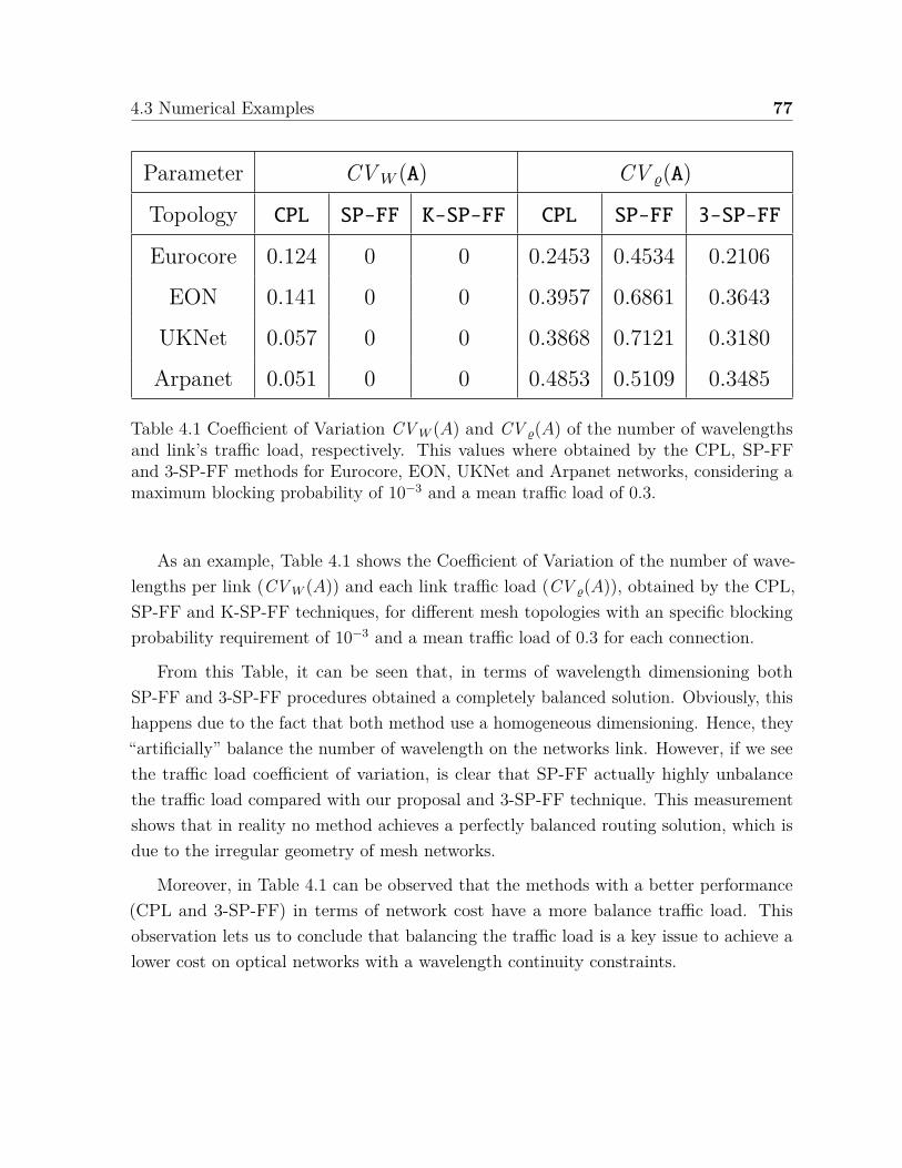
4.3 Numerical Examples 77
Parameter CV W (A) CV ϱ(A)
Topology CPL SP-FF K-SP-FF CPL SP-FF 3-SP-FF
Eurocore 0.124 0 0 0.2453 0.4534 0.2106
EON 0.141 0 0 0.3957 0.6861 0.3643
UKNet 0.057 0 0 0.3868 0.7121 0.3180
Arpanet 0.051 0 0 0.4853 0.5109 0.3485
Table 4.1 Coefficient of Variation CV W (A) and CV ϱ(A) of the number of wavelengthsand link’s traffic load, respectively. This values where obtained by the CPL, SP-FFand 3-SP-FF methods for Eurocore, EON, UKNet and Arpanet networks, considering amaximum blocking probability of 10−3 and a mean traffic load of 0.3.
As an example, Table 4.1 shows the Coefficient of Variation of the number of wave-lengths per link (CV W (A)) and each link traffic load (CV ϱ(A)), obtained by the CPL,SP-FF and K-SP-FF techniques, for different mesh topologies with an specific blockingprobability requirement of 10−3 and a mean traffic load of 0.3 for each connection.
From this Table, it can be seen that, in terms of wavelength dimensioning bothSP-FF and 3-SP-FF procedures obtained a completely balanced solution. Obviously, thishappens due to the fact that both method use a homogeneous dimensioning. Hence, they“artificially” balance the number of wavelength on the networks link. However, if we seethe traffic load coefficient of variation, is clear that SP-FF actually highly unbalancethe traffic load compared with our proposal and 3-SP-FF technique. This measurementshows that in reality no method achieves a perfectly balanced routing solution, which isdue to the irregular geometry of mesh networks.
Moreover, in Table 4.1 can be observed that the methods with a better performance(CPL and 3-SP-FF) in terms of network cost have a more balance traffic load. Thisobservation lets us to conclude that balancing the traffic load is a key issue to achieve alower cost on optical networks with a wavelength continuity constraints.
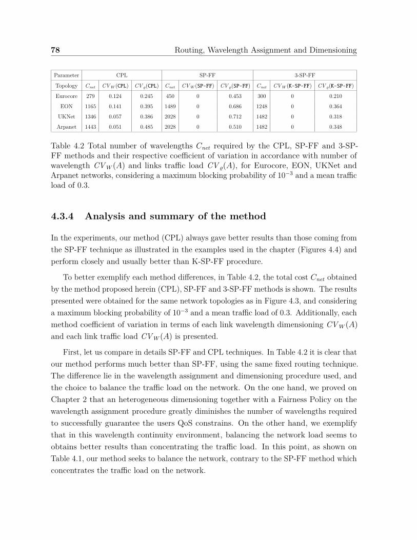
78 Routing, Wavelength Assignment and Dimensioning
Parameter CPL SP-FF 3-SP-FF
Topology Cnet CV W (CPL) CV ϱ(CPL) Cnet CV W (SP-FF) CV ϱ(SP-FF) Cnet CV W (K-SP-FF) CV ϱ(K-SP-FF)
Eurocore 279 0.124 0.245 450 0 0.453 300 0 0.210
EON 1165 0.141 0.395 1489 0 0.686 1248 0 0.364
UKNet 1346 0.057 0.386 2028 0 0.712 1482 0 0.318
Arpanet 1443 0.051 0.485 2028 0 0.510 1482 0 0.348
Table 4.2 Total number of wavelengths Cnet required by the CPL, SP-FF and 3-SP-FF methods and their respective coefficient of variation in accordance with number ofwavelength CV W (A) and links traffic load CV ϱ(A), for Eurocore, EON, UKNet andArpanet networks, considering a maximum blocking probability of 10−3 and a mean trafficload of 0.3.
4.3.4 Analysis and summary of the method
In the experiments, our method (CPL) always gave better results than those coming fromthe SP-FF technique as illustrated in the examples used in the chapter (Figures 4.4) andperform closely and usually better than K-SP-FF procedure.
To better exemplify each method differences, in Table 4.2, the total cost Cnet obtainedby the method proposed herein (CPL), SP-FF and 3-SP-FF methods is shown. The resultspresented were obtained for the same network topologies as in Figure 4.3, and consideringa maximum blocking probability of 10−3 and a mean traffic load of 0.3. Additionally, eachmethod coefficient of variation in terms of each link wavelength dimensioning CV W (A)and each link traffic load CV W (A) is presented.
First, let us compare in details SP-FF and CPL techniques. In Table 4.2 it is clear thatour method performs much better than SP-FF, using the same fixed routing technique.The difference lie in the wavelength assignment and dimensioning procedure used, andthe choice to balance the traffic load on the network. On the one hand, we proved onChapter 2 that an heterogeneous dimensioning together with a Fairness Policy on thewavelength assignment procedure greatly diminishes the number of wavelengths requiredto successfully guarantee the users QoS constrains. On the other hand, we exemplifythat in this wavelength continuity environment, balancing the network load seems toobtains better results than concentrating the traffic load. In this point, as shown onTable 4.1, our method seeks to balance the network, contrary to the SP-FF method whichconcentrates the traffic load on the network.

4.3 Numerical Examples 79
Next, lets compare K-SP-FF and our method. As presented on the figure 4.4 andTable 4.2 CPL obtains slightly better results than K-SP-FF, in accordance with the Cnet
value obtained, but using a simpler routing scheme. Both algorithm achieves a muchmore balance solution than SP-FF, reenforcing us the idea that a balance solution obtainsa better performance in terms of network cost. On top of this, as previously explained,K-SP-FF technique uses a fixed alternate routing scheme, thus it provides connectivityusing K alternate routes to transmit, contrary to the CPL method which uses only onepath to communicate each user. This means, that our technique performs similar thana more complex technique on several points (as mention on subsection 4.3.2). First,K-SP-FF requires K times memory size to store the routing tables, since it requires tostore K routes per network user. Additionally, the delay induced by the routing procedureis bigger than our method, due to the fact that it requires to read the routing table moretimes per connection attempt to transmit on any alternate route available.
Let us discuss here some qualitative reasons that justify the better results of CPLover SP-FF and K-SP-FF:
• By simultaneously solving the 2 problems (routing, and wavelengths dimensioning),a global solution is obtained, which is a more efficient strategy than to solve theseproblems separately.
• The routing strategy is based on fixed routing, defining one path to each userprevious the network operation and stored in routing tables. This solution is basedon our hypothesis that a fixed routing can perform as good as fixed alternaterouting (or even better). This can be possible if we pre-compute proper routes toeach network connection, and dimension the network simultaneously with the routeselection. This joint solution allow us to take advantage of statistical decisions, byexploring a bigger solution space to find the best possible solution. To do this, werely on the fast and accurate analytical blocking probability evaluation proposedin Chapter 2, allowing us to make better decisions than other heuristic solutionsbased on simulation techniques.
• The dimensioning procedure assigns a different number of wavelengths to eachnetwork link (called Heterogeneous Dimensioning), such that the blocking probabilityof each connection does not exceed a predefined maximum blocking probability.
80 Routing, Wavelength Assignment and Dimensioning
This takes advantage that real network are hardly symmetric, thus hard to balancethe connections traffic load within.
• Additionally, the dimensioning procedure uses a wavelength assignment policy called“Fair Policy”. This policy consists in to offer a maximum blocking probability to eachnetwork user as close as possible to the one defined in the SLA, since each user mayhave different quality of service requirements. This way the method diminishes thewavelength dimensioning since each connection uses only the wavelengths neededto satisfy their QoS demand.
• The usual blocking probability evaluation technology is based on simulation, whichis a slow procedure. Consequently, the evaluation process is limited to only a fewrestricted scenarios. So, to find the best possible solution, researchers apply somecriteria to restrict the solutions search (heuristics), for example, making choicesas the shortest path. CPL obtains better results, so we can conclude that suchheuristic solutions are not using good assumptions and taking appropriate decisions.
• The routing method balances the traffic load on the network. This is due tothe relative cost function defined to decide each user path. As mentioned on thenumerical results, we conclude that this characteristic is a key aspect to achievea lower cost in terms of wavelength dimensioning, while satisfying the quality ofservice predefined on the SLA at the same time.
In addition to the increased efficiency compared to existing methods, the CPL methodhas other desirable attributes:
• The on-line operation (during network operation) of the method is very fast andsimple. This is due to the fact that our proposal uses a fixed routing scheme, andthe routing information is stored in routing tables, which contain each connection’spath. This means that the routing mechanism is as short as possible.
• The off-line execution time of the CPL method takes only a few seconds using astandard current PC (Windows 10 64 bits, Intel Core i7 2.60GHz processor and8GB RAM).
4.4 Conclusions 81
4.4 Conclusions
A new method was proposed to jointly solve three of the main problems in optical networkdesign: it determines the set of routes enabling each network user to transmit, it definesan efficient wavelength assignment scheme in order to choose a wavelength to transmiton each communication request, and it evaluates the minimum number of wavelengthsnecessary on each network link while guaranteeing certain blocking probability thresholdto each user (which is a design parameter of the network).
The technique proposed is considerably different from those published so far. Itcomputes a global solution, which often obtains a better solution than solving theproblems separately. In fact, it obtains better results in terms of number of wavelengthsassigned to the links (specially than the fixed routing method known as SP-FF), withless entries on the routing tables than any fixed alternate routing method. Hence, CPLrequires less memory to store the paths on the routing tables, and it involves a smallerdelay to route each user each time it attempts to transmit.
It is important to notice that the proposal obtains on average 20% less wavelengththan required on the static operation scenario. This results may provide enough reasonsto migrate from static to dynamic operation.
Due to the fact that our methods use the procedure proposed on chapter 3, themethod assigns different number of wavelengths on each link (heterogeneous wavelengthdimensioning), and defines a Fairness policy in the First-Fit Wavelength Assignment, inorder to offer a quality of service to each user as close as the one requested on the ServiceLevel Agreement.
The method is executed previous the network operation requiring a few seconds tosimultaneously solve the R&WAD problem. Additionally, the network operation basedon our approach is simple and fast, due to the fact that the paths are stored in routingtables and addressed on demand.


Chapter 5
Fault Tolerance
5.1 Introduction
Another issue to be solved in order to design WDM optical networks is to ensure thatthe network will still be able to provide its transmission service after the failure of oneor more of its links. The solution to this problem consists in providing the necessaryinfrastructure to rapidly re-establish communications between all source-destination pairof nodes affected by these link failures. This type of mechanism is known as “FaultTolerance”.
The frequency of link failures’ occurrences is often significant. For instance, [29, 30]reports measures of the mean time between failures of about 367 year/km. This explainswhy failures on links may significantly impact the performance of the networks. Forexample, in a 26,000 km-long network such as NSFNet [91], there is an average of onefiber cut every 5 days. Moreover, it has been found that the frequency with which twosimultaneous network failures occur is high enough to be taken into account in the designprocess. For example, in [30] it has been reported that the probability of two simultaneousfailures occurring in a network like NSFNet is approximately 0.0027 (a downtime ofabout 24 hours per year on average), which in addition to the high transmission rate ofthis kind of networks, implies an unacceptable loss for the operator if the event happens.
The previous elements justify the need to provide an efficient methodology for multiplefault tolerance, which should ensure (with a certain probabilistic guarantee) successful
84 Fault Tolerance
communications among all network users, despite the occurrence of failures in some ofthe links, and at the lowest possible cost regarding the network infrastructure.
The fault tolerance methods proposed so far generally have been devoted to findingalternative paths considering single link failure. This means, one bidirectional link fails,affecting the connections with routes passing through the failed link in both directions(uplink and downlink). Then, the number of wavelengths in the network is dimensionedto tolerate this situation [30, 92, 93]. However, as already noted, the probability ofoccurrence of two or more simultaneous failures is often high enough, making that it isuseful to consider this event in the design of the network. Some studies have focusedon this scenario [94–97], which are described next. Also, some studies have considerspecial cases of failure, such as Disaster risk constrains and Shared-Risk-Group scenarios.Disaster risk constrains [98, 99] considers the possible service disruptions in case of anatural disaster or a targeted attack. On the other hand, Shared-Risk-Group (SRG) [100]considers the possibility that some fibers are placed physically together, even if they areconnecting different optical nodes. This scenario makes them all liable to physical cuts,since they can be cut together at the same time.
Let us briefly list next the most common methods currently used to provide faulttolerance. One of the most frequent ways considered to address simple and double faulttolerance, called “1+1”, can be found in [101, 43, 102, 103, 92, 104]. In this technique,a secondary route is associated with each primary one (with the restriction that theydon’t share any link) and the information is transmitted simultaneously through bothof them. To dimension the number of wavelengths of each link (task usually done bysimulation), each secondary route is considered as just another network route with a loadequal to the corresponding primary one. The 1+1 method is also scalable to providetolerance to K ≥ 1 simultaneous failures. In this case, for each connection, K + 1supplementary disjoint routes must be found, one to be designed as the primary route andthe remaining K as secondary routes. Observe that a necessary and sufficient condition(allowing this scheme to work) is that the graph defined by the set of nodes and links is(K + 1)-connected.
Another strategy is described in [105], where a routing technique is proposed toprovide fault tolerance while sharing the resources of the network. This method is knownas “Shared Path Protection” (SPP) [106, 105, 107]. In this method the extra resources(wavelengths) assigned to the secondary routes can be shared by different connections,
5.1 Introduction 85
and are assigned only when a fault occurs. It can be executed in two different ways. Thefirst one consists of running the algorithm off-line, where the routes are calculated prior tothe operation of the network (off-line SPP). The second way is the on-line implementation(on-line SPP). In this last case, the method is executed every time there is a network linkfailure. In the SPP online mode, the primary routes are specified before the network isoperating, but in order to find new routes to the affected connections it must be executedagain every time that one or more simultaneous failures occur. For this reason, we saythat this is a proactive and a reactive approach at the same time.
Finally, in [108–110, 94–96] a method of fault tolerance called “p-cycle” is used,allowing sharing resources through fixed secondary routes which have a cyclic form. Theseroutes are shared between several primary routes. One problem with this approach isthat the applicability of the idea is very dependent on the size of the network, introducingexcessive additional delay for a connection in protection state on large networks. Also,to perform multiple fault tolerance, this method requires a large amount of cycles (e.g.hundreds of cycles for the 11 nodes pan-European COST 239 network [109]), which isimpractical from various points of view.
In this chapter we propose a new procedure for simultaneously solve the routing,wavelength assignment, wavelength dimensioning and multiple fault tolerance problems(which we call the “Cheapest Path By Layers with Fault Tolerance” method- CPLFT ).This new approach obtains all primary and secondary routes assigned to each possibleconnection. Secondary routes replace the primary ones when the latter are affected byat least one failure, thus keeping users connected as long as the network itself remainsconnected; that is, for every connection (user) there is at least one path with operationallinks to reach their destination nodes. In our approach we go one step further, and wetake into account the case of an arbitrary set of simultaneous failures. The method alsoevaluates the number of wavelengths Wℓ for each link ℓ of the network, ensuring thatthe blocking probability of any connection request will be lower than the predefinedthreshold βc previously mentioned, despite the possible occurrence of those simultaneouslink failures. The technique relies on a wavelength assignment and dimensioning completelydifferent than the ones proposed to date. It introduces 2 new features: the number ofwavelengths (in general) are different on each link (heterogeneous dimensioning); and thewavelength assignment used introduces a Fairness Policy to each network user providinga quality of service as close as possible as the one defined on the SLA.

86 Fault Tolerance
The remainder of this chapter is as follows: Section 5.2 presents the new algorithm.Section 5.3 contains some results obtained by the proposed algorithm, which are comparedwith those obtained with the current best methods in a set of different scenarios. Finally,the conclusions of the study are given in Section 5.4.
5.2 Fault tolerance strategy
This section contains the main contribution of the chapter. We present first the modelused and the related assumptions. Then, we describe the main sub-procedures necessaryto our technique. Last, we present the fault tolerance algorithm.
5.2.1 Model and assumptions
We define the same model and assumptions than previous chapters. Thus, if you arealready familiar with it, you are welcome to skip this sub-section and continue in FaultTolerance definitions 5.2.1.
The network topology is represented by a graph G = (N ,L), where N is the set ofnetwork nodes or vertices and L is the set of unidirectional links (the arcs in G), withrespective cardinalities |N | = N and |L| = L. The set of connections X ⊆ N 2, withcardinality |X | = X, is composed by all the source-destination pairs with communicationbetween them. These connections are also called “users” in the text.
To represent the traffic between a given source-destination pair, an ON-OFF model isused. Consider connection c. During any of its ON periods, whose average length is tON c,the source transmits at a constant rate (which is the rate associated to the wavelength).During an OFF period, with average length tOFF c, the source refrains from transmittingdata.
To simplify the presentation, the constant transmission rate during the ON periods isdetermined by the used technology, that will be our rate unity. Consequently, the trafficload of connection c, denoted by ϱc, is given by the following expression:
ϱc = tON c
tON c + tOFF c
. (5.1)

5.2 Fault tolerance strategy 87
Observe that we address here the general case where the load can be different for eachconnection, the so-called heterogeneous situation, instead of the usual homogeneous casewhere the load is assumed to be the same for all users [74, 111–113, 95, 114, 96, 115–117].
Let R = rc | c ∈ X be the set of routes that enable communications among thedifferent users, where rc is the route associated with connection c ∈ X . The set R isalso denominated set of primary routes, because this set alone does not offer any faulttolerance to the possible failure of network links.
LetW = Wℓ | ℓ ∈ L be the set containing the number of wavelengths associated witheach unidirectional network link, where Wℓ, ℓ ∈ L, is the number of wavelengths on link ℓ.The value Wℓ, for every ℓ ∈ L, will be evaluated so that the blocking probability BPc ofeach connection c ∈ X is less than or equal to a given pre-specified threshold βc and thetotal number of available network wavelengths is as small as possible. Remark that thepre-defined threshold value βc can be different for each network connection, allowing themethod to solve these problems when there are classes of users with different priorities.
As in previous chapters, in this work the total network cost Cnet is defined as the sumof all wavelengths of all network links, that is, Cnet = ∑
ℓ∈L Wℓ. As we are consideringfault tolerance capabilities, this includes all the extra wavelengths needed to providetolerance to multiple link failures.
Fault tolerance definitions
Consider a set of every possible failure scenarios Ω on the network to be considered. Eachof these scenarios is a subset of failed network links F , where F ⊂ L. This subset Fcorresponds to a failure scenario, where every links belonging to F is non-operational(failed). Therefore, this method can be applied to any possible case of failures in thenetwork, e.g.: every possible single failure scenario (|F| = 1) which corresponds to thecase of single link failure; every possible double failure scenario (|F| = 2); node failure(corresponding to a special case of multiple failure, where all the links connected to thatnode are non-operational); Disaster risk constrains [98, 99] can be considered in ourmethod by including in the failure scenario F all the links where the disaster has takenplace; also, Shared-Risk-Group (SRG) [100] can be considered also as a special case ofmultiple link failures, where F is composed by every link that can be affected by thesame physical cut.
88 Fault Tolerance
Assume some failure scenario F is also given (or observed), that is, assume that thelinks in F are failed, and those that don’t belong to F work (are operational). Someadditional definitions required for this method are presented in the following list:
• G−F = (N ,L \ F), is the partial graph of G (same nodes, part of the edges),containing only the non-failed links;
• XF = c ∈ X | there exists ℓ ∈ F with ℓ ∈ rc, is the set of all network connectionswhose routes pass through at least one failed link;
• AF = rc ∈ R | there exists ℓ ∈ F with ℓ ∈ rc, is the set of routes that areaffected when all links in F fail; that is, AF is the subset of the routes in R thatare associated with the connections in XF ;
• RF is a set of routes that replace those in AF when all links in F are failed; foreach of these routes, the corresponding blocking probability must be less than orequal to the corresponding given upper bound;
• SF is the total set of routes guaranteeing fault tolerance to the failure event “alllinks in F fail”, that is, the set defined by SF =
(R \ AF
)∪RF .
• CF = Cℓ | for all L \ F is the total set of costs of each link non-affected by afailure.
5.2.2 Sub-procedures needed by our CPLFT method
The method needs a few sub-procedures to work. They are described next. Since thegiven graph and the set of connections (or users) are fixed data that never change, aswell as the upper bounds βc of the blocking connection probabilities, we will omit themin the list of the parameters of the procedures. Also, when we refer to the network cost,we will write simply Cnet because we must in general change many times during thecomputational process the capacities of the links.
PrimaryRoutes(): initial computation of primary routes Our method starts bycomputing an initial set of routes and the corresponding wavelength dimensioning. Thisare the primary routes by which each connection normally transmits its information. This

5.2 Fault tolerance strategy 89
can be done by any available technique. Nevertheless, for each connection (s, t) we lookfor the cheapest routes from nodes s to t in the graph, using the algorithm propose onchapter 4. The algorithm, called CPL, propose a novel technique to simultaneously solvethe routing, wavelength assignment and wavelength dimensioning. The method assigns toeach source-destination pair of nodes the cheapest path while trying to balance the trafficload on each network link. The method also evaluates the number of wavelengths Wℓ
for each link ℓ of the network, ensuring that the blocking probability of any connectionrequest will be lower than the predefined threshold βc, and introduces a Fairness Policy onthe wavelength assignment solution, defining a scheme to assign on demand a wavelengthto transmit on each attempt of communication.
Let us symbolically write R,W := PrimaryRoutes() to represent the execution ofthis sub-procedure.
SecondaryRoutes(): given the set of link failures, find new routes The problemis the following: we have a set of failure links F , the set of costs CF and a set of users XF
affected by the failure of the links in F . We would like to find a new set of routes allowingto connect each user in XF in case of the failure scenario F , while still satisfying the QoSrequired by each connection.
The search for new routes is then done as follows. We run Dijkstra’s algorithmslooking, for each user c ∈ X , for the cheapest route where the link costs are now given bythe link costs in CF (explained on the algorithm). This produces a new set of routes thatwe denote RF .
Symbolically, we execute the call RF := SecondaryRoutes(XF ,F , CF).
WavelengthAD(): given the routes and the thresholds βc, compute the capacitiesWe call WavelengthAD this sub-procedure (“Wavelength Assignment and Dimensioning”).The problem consists in finding, for each link ℓ ∈ L, a capacity Wℓ such that the end-to-end blocking probability BPc of every user c ∈ X passing through the link ℓ is less thanthe given threshold or upper bound, denoted as βc, while at the same time, providing awavelength assignment scheme to use during the network operation. The routes R areconsidered fixed and calculated before the evaluation of this sub-procedure.
90 Fault Tolerance
The wavelength assignment method is based on the First-Fit method, due it is thefastest and simplest method with a good performance in terms of blocking probability,but will be modified to a better match between the QoS offered and the QoS actuallyobtained on the network.
To dimension the wavelengths on each network link, and to define a proper wavelengthassignment strategy, we use the method proposed on the chapter 3. The method wascalled Fair-HED. First, Fair-HED method introduces a “Fairness Policy” to solve thewavelength assignment. This policy is based on the First-fit approach, but the numberof wavelengths available to each connection are different (defined on the method itselfand stored in the set U = uc | c ∈ X). This Fairness policy allows a tighter differencebetween the quality of service offered to each user and the QoS requested on the SLA.Second, the dimensioning procedure assigns a different number of wavelengths on each link,called “Heterogeneous Dimensioning”, while satisfying a predefined maximum blockingprobability given on the SLA βc.
For additional information about this sub-procedure, chapter 3 addresses the wave-length assignment and dimensioning technique used in this procedure.
Let us symbolically write W ,U = WavelengthAD(L,R) to represent the evaluationof this sub-procedure.
5.2.3 R&WAD+FT procedure
The routing, wavelength assignment, wavelength dimensioning and fault tolerance(R&WAD+FT) problems consists in finding, for each connection a primary route to befollowed by the data to be transmitted, additional routes (also called secondary route)used to keep each user connected in cases where one or more simultaneous failures occur,and at the same time, to find, for each link ℓ ∈ L, a strategy to assign on demand eachuser wavelength to communication and a capacity Wℓ, such that the end-to-end blockingprobability BPc of every user c ∈ X passing through the link ℓ is less than the giventhreshold or upper bound βc, despite the occurrence of link failures.
These tasks are usually solved separately [10]. This happens due to the fact thatsolving them simultaneously have a great complexity associated. By solving separatelythe Routing, the Wavelength Assignment, Wavelength Dimensioning and Fault tolerance

5.2 Fault tolerance strategy 91
Fig. 5.1 Diagram showing the inputs required to run the CPLFT method, the conditionto be guarantee by the method, and the outputs delivered by the method, to solve therouting and wavelength dimensioning problem.
is possible to achieve good local solutions to each problem. As shown on previouschapters, we strongly believe that to provide a joint solution of the R&WAD+FT problemmay achieve a good global solution. As a matter of fact, recently in [118, 119], anexhaustively validated heuristic strategy, called Joint3 was applied, solving jointly therouting, wavelength dimensioning and fault tolerance problems, in the context of WDMoptical networks with wavelength conversion capabilities. Its performance was betterthan local strategies approaches.
We named the method proposed herein “Cheapest Path by Layers considering FaultTolerance” (CPLFT).
Figure 5.1 presents a diagram presenting the inputs required by the method, thecondition to be guarantee by the method and the outputs obtained by the methodexecution. In figure 5.1 the inputs are: the network topology G = (N ,L), which canbe any network topology; each user traffic load ϱc, for all connections in X , offered tothe network. Notice that, the value ϱc of each user c can be different, we called this“Heterogeneous traffic load”; and the set Ω = F|F ⊂ L composed by all the link failurescenarios to be considered by the method execution. The requirement to be satisfied bythe method is to guarantee a maximum blocking probability to each network user βc,predefined on the Service Level Agreement (SLA). Finally, the method’s outputs are theset of routes R allowing to provide communication to each network connection c, for all
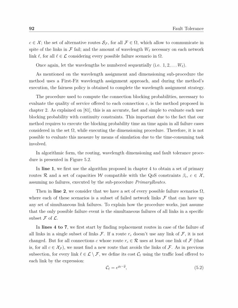
92 Fault Tolerance
c ∈ X ; the set of alternative routes SF , for all F ∈ Ω, which allow to communicate inspite of the links in F fail; and the amount of wavelength Wℓ necessary on each networklink ℓ, for all ℓ ∈ L considering every possible failure scenario in Ω.
Once again, let the wavelengths be numbered sequentially (i.e. 1, 2, . . . Wℓ).
As mentioned on the wavelength assignment and dimensioning sub-procedure themethod uses a First-Fit wavelength assignment approach, and during the method’sexecution, the fairness policy is obtained to complete the wavelength assignment strategy.
The procedure used to compute the connection blocking probabilities, necessary toevaluate the quality of service offered to each connection c, is the method proposed inchapter 2. As explained on [81], this is an accurate, fast and simple to evaluate each userblocking probability with continuity constraints. This important due to the fact that ourmethod requires to execute the blocking probability time an time again in all failure casesconsidered in the set Ω, while executing the dimensioning procedure. Therefore, it is notpossible to evaluate this measure by means of simulation due to the time-consuming taskinvolved.
In algorithmic form, the routing, wavelength dimensioning and fault tolerance proce-dure is presented in Figure 5.2.
In line 1, we first use the algorithm proposed in chapter 4 to obtain a set of primaryroutes R and a set of capacities W compatible with the QoS constraints βc, c ∈ X ,assuming no failures, executed by the sub-procedure PrimaryRoutes.
Then in line 2, we consider that we have a set of every possible failure scenarios Ω,where each of these scenarios is a subset of failed network links F that can have upany set of simultaneous link failures. To explain how the procedure works, just assumethat the only possible failure event is the simultaneous failures of all links in a specificsubset F of L.
In lines 4 to 7, we first start by finding replacement routes in case of the failure ofall links in a single subset of links F . If a route rc doesn’t use any link of F , it is notchanged. But for all connections c whose route rc ∈ R uses at least one link of F (thatis, for all c ∈ XF), we must find a new route that avoids the links of F . As in previoussubsection, for every link ℓ ∈ L \ F , we define its cost Cℓ using the traffic load offered toeach link by the expression:
Cℓ = eϱℓ−ϱ, (5.2)

5.2 Fault tolerance strategy 93
function CPLFT()// --- input: the graph (the network), the connections,// the bounds on the blocking probabilities,// and the set Ω of links failure scenarios,// where at most one of the events ‘all links in F// fail simultaneously’ occurs, all seen as global variables// --- output: the primary routes, the secondary routes// and the wavelengths per link
// first compute primary routes and corresponding dimensioning1 (R,W) := PrimaryRoutes();
// calculates secondary paths in all failure scenarios.2 foreach F in Ω3 for all links ℓ ∈ L \ F4 ϱℓ :=
∑c∈X \XF ∧ℓ∈rc
ϱc; // non-affected routes
5 ϱ :=
∑ℓ∈L\F ϱℓ
L ;6 Cℓ := eϱℓ−ϱ;7 RF := SecondaryRoutes(XF ,F , CF); // compute alternative routes8 SF :=
(R \ AF
)∪RF;
9 WF := WavelengthAD(L \ F ,SF);
// Decide the final wavelength dimensioning10 for all links ℓ ∈ L11 Wℓ := Max(Wℓ,W1,ℓ, ..W|Ω|,ℓ)12 return (R,S,W)
Fig. 5.2 Algorithm for solving the R&WAD problem, providing alternative routes if thelinks of one specific subset of links fail (all together) belonging to a list of possible subsetsof links that can fail.
where ϱℓ is the traffic load offered to the link ℓ by the connections non-affected by thefailed links, and ϱ is the mean traffic load on the operational links L \ F . Then, withthese Cℓs as weights, we run Dijkstra’s algorithm to find the cheapest route for eachconnection c ∈ XF . The set of all these routes will be denoted by RF . Symbolically, weexecute the call RF := SecondaryRoutes(XF ,F , CF).

94 Fault Tolerance
Then, line 8 defines the set of routes SF :
SF =(R \ AF
)∪RF .
In words, SF is the set of routes to use when all links in F are failed. Now, we mustdimension again the links because we must always respect the QoS constraints. For thispurpose, we restrict the analysis to the graph G−F , that is, we remove the links in Ffrom L, and in line 9 we run a dimensioning phase. In pseudo-algorithmic form, weexecute the function call WF := Dimensioning(L \ F ,SF).
To finish this process in lines 10 to 11, since we obtain now new capacities for thelinks WF ,ℓ, for every possible failure scenario in Ω, we compare each WF ,ℓ (and the Wℓ
obtained in the no failure scenario), for all ℓ ∈ L, and the final capacity of the link willbe the maximum between them. Formally, we add a procedure Max() that performs thistask, and we symbolically write Wℓ := Max(Wℓ,W1,ℓ, ..W|Ω|,ℓ). Finally, putting togethereach final link capacity Wℓ, ℓ ∈ L will conform the final dimensioning set W .
The complexity of the fault tolerance procedure presented on Fig 5.2 is proportionalto the number of link failures scenarios in Ω, the complexity of Dijkstra’s algorithm(O(N2)) to find the cheapest routes for every connection in XF and the algorithmic costto execute the dimensioning procedure (define as O(W )). The set XF cardinality is givenby X the total number of network connections, multiplied by the mean number of hopsof each connection route, which is denoted by r, divided by the total number of networklinks L. Then, the procedure complexity is order O(|Ω|N2X · r/LW ). For example, inthe case of single link failure (in this case the number of link failures scenarios |Ω| is givenby the L possible single link failure) the complexity of the proposed method is orderO(LN2X · r/LW ). On the other hand, if the algorithm is used to solve the problemof double link failures, the link failure scenarios are |Ω| = L2; therefore the algorithmcomplexity is order O(L2N2X · r/LW ).
5.3 Numerical Examples
To quantify the quality of the solution obtained by the CPLFT method, it should becompared against the optimal solution. However, it is known that the R&WAD problemis an NP-complete problem [90]. Those who have been dedicated to solve this problem
5.3 Numerical Examples 95
optimally only have been able to achieve it to very small networks (with less than 10 nodes).Consequently, for real network topologies (dozens to hundreds nodes) the fault toleranceproblem cannot be optimally solved. Given this situation, our best alternative was tocompare the CPLFT method with those methods considered as the most competitive atthis moment.
Then, it is necessary to make the comparison using metrics that enable to assess theadvantages/disadvantages of each fault tolerance method. The most important metricsfor the routing, wavelength assignment, wavelength dimensioning and fault tolerancemethods are: the cost of the network and the delay in the restoration procedure incase of the occurrence of failures, when this is relevant (in our approach this delay iscomparable to the time needed to access the primary routes on the routing tables sincethe computations are done off-line).
When reviewing the current methods of Routing and Wavelength Assignment, itwas noted that the algorithms most commonly referenced today, and considered thebest so far, use the shortest path (both fixed and fixed alternate routing strategy)together with a First Fit wavelength assignment scheme. These are SP-FF and K-SP-FF [16, 10, 88, 85, 5, 9, 86, 11, 12] (see Chapter 4 Section 4.1). It is interesting to considerthat the K-SP-FF technique is a fixed alternate routing method, thus it uses severaldisjoint alternative routes to provide communication. By itself, it provides certain level offault tolerance, thanks to the alternative routes, but it does not guarantee fault tolerance.This occurs due to the fact that K-SP-FF requires to define a restoration proceduretogether with a dimensioning procedure which calculates the extra resources needed toguarantee fault tolerance on diverse scenarios. Nevertheless, if we adjust the K-SP-FF toprovide fault tolerance satisfying the QoS restrictions, then the result would be the sameas to add fault tolerance to the SP-FF method. Consequently, SP-FF was the routingmethod chosen for comparison.
Additionally, as it was explained on Chapter 3 and 4, the Wavelength Dimensioningmethod most commonly used is the homogeneous dimensioning. Consequently, we willconsider an homogeneous dimensioning with the SP-FF method.
There are several types of fault tolerance algorithms proposed so far, such as SharedPath Protection, p-cycle and 1+1. In the sequel we discuss the pertinence in comparingCPLFT with each of these different types of algorithms.

96 Fault Tolerance
Shared Path Protection (SPP) Method This strategy provides tolerance to mul-tiple network links failure. There are two methods for implementing this algorithm(SPP on-line and SPP off-line). Both methods require between 40 to 80% of additionalwavelengths (compared to the case without fault tolerance) to provide single link faulttolerance capability [105]. Another aspect that must be considered is that the SPPoff-line method has the additional weakness that the percentage of restorability obtained(percentage of connections that remain connected in case of link failure) is very low (80%to 90% [105]). Therefore, it is not comparable to the method proposed in this work, whichensures that the blocking probability pre-established by the network designer (i.e. 10−6)is satisfied. On the other hand, the implementation of the SPP-online method requires torun on demand a route search algorithm (whenever one or more links fail) in order to findan alternative route to each affected connection. Evidently, this on-line strategy causes aslow re-routing, which added to the fact that many of the applications that use computernetworks require very fast on-line responses in case of failures [28], make that this typeof method does not represent a practical fault tolerant mechanism for many practicalapplications. Due to the facts just commented, the SPP method was not considered forcomparison with the method proposed in this paper.
The p-cycle Method To provide tolerance to multiple failures, this method requiresa large quantity of cycles (which implies a high cost when defining secondary routes), soit is not scalable for multiple faults. Given the fact that in this paper we consider themultiple fault tolerant case, it is unreasonable to compare our method with the p-cycleone.
Method 1+1 This method provides tolerance to multiple failures, using as manydisjoint routes as simultaneous link failures it can tolerate. It solves the problem ofprimary and secondary routes prior to the network dimensioning (off-line) sub-task.Then, the number of wavelengths is computed, having as a constraint to provide enoughresources to all routes, and guaranteeing sufficient information to re-route each connectionin case of failure. Consequently, 1+1 is the most suitable fault tolerance method tocompare with our algorithm.
In summary, the most appropriate methods for comparison are SP-FF in order togenerate the primary routes and then, 1+1 for the fault tolerance mechanism. These two

5.3 Numerical Examples 97
Fig. 5.3 Mesh networks evaluated. The number of links refers to the number of bidirectionalarcs. Observe that in the picture we see the edges (for instance, the picture shows theEurocore topology with 25 edges, which corresponds to 50 arcs). The parameter dis a measure of density: if the graph has a arcs (twice the number of edges) and n
nodes, d = a/(n(n− 1)
).
methods together are denoted SPFF1+1 in the chapter. To evaluate the correspondingblocking probabilities, the mathematical method proposed in chapter 2 was used in bothSPFF1+1 and CPLFT.
To evaluate the performance of the methods under different scenarios, the algorithmswere executed for different real network topologies, having different sizes and differentdegrees of connection d, where d is the average number of neighbors of a node in thenetwork. Some of the selected topologies and their respective parameters N , L and d areshown in Figure 5.3.
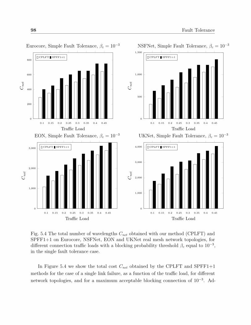
98 Fault Tolerance
0.1 0.15 0.2 0.25 0.3 0.35 0.4 0.450
200
400
600
800
Traffic Load
Cne
t
Eurocore, Simple Fault Tolerance, βc = 10−3
CPLFT SPFF1+1
0.1 0.15 0.2 0.25 0.3 0.35 0.4 0.450
500
1,000
1,500
Traffic LoadC
net
NSFNet, Simple Fault Tolerance, βc = 10−3
CPLFT SPFF1+1
0.1 0.15 0.2 0.25 0.3 0.35 0.4 0.450
1,000
2,000
3,000
Traffic Load
Cne
t
EON, Simple Fault Tolerance, βc = 10−3
CPLFT SPFF1+1
0.1 0.15 0.2 0.25 0.3 0.35 0.4 0.450
1,000
2,000
3,000
4,000
Traffic Load
Cne
t
UKNet, Simple Fault Tolerance, βc = 10−3
CPLFT SPFF1+1
Fig. 5.4 The total number of wavelengths Cnet obtained with our method (CPLFT) andSPFF1+1 on Eurocore, NSFNet, EON and UKNet real mesh network topologies, fordifferent connection traffic loads with a blocking probability threshold βc equal to 10−3,in the single fault tolerance case.
In Figure 5.4 we show the total cost Cnet obtained by the CPLFT and SPFF1+1methods for the case of a single link failure, as a function of the traffic load, for differentnetwork topologies, and for a maximum acceptable blocking connection of 10−3. Ad-
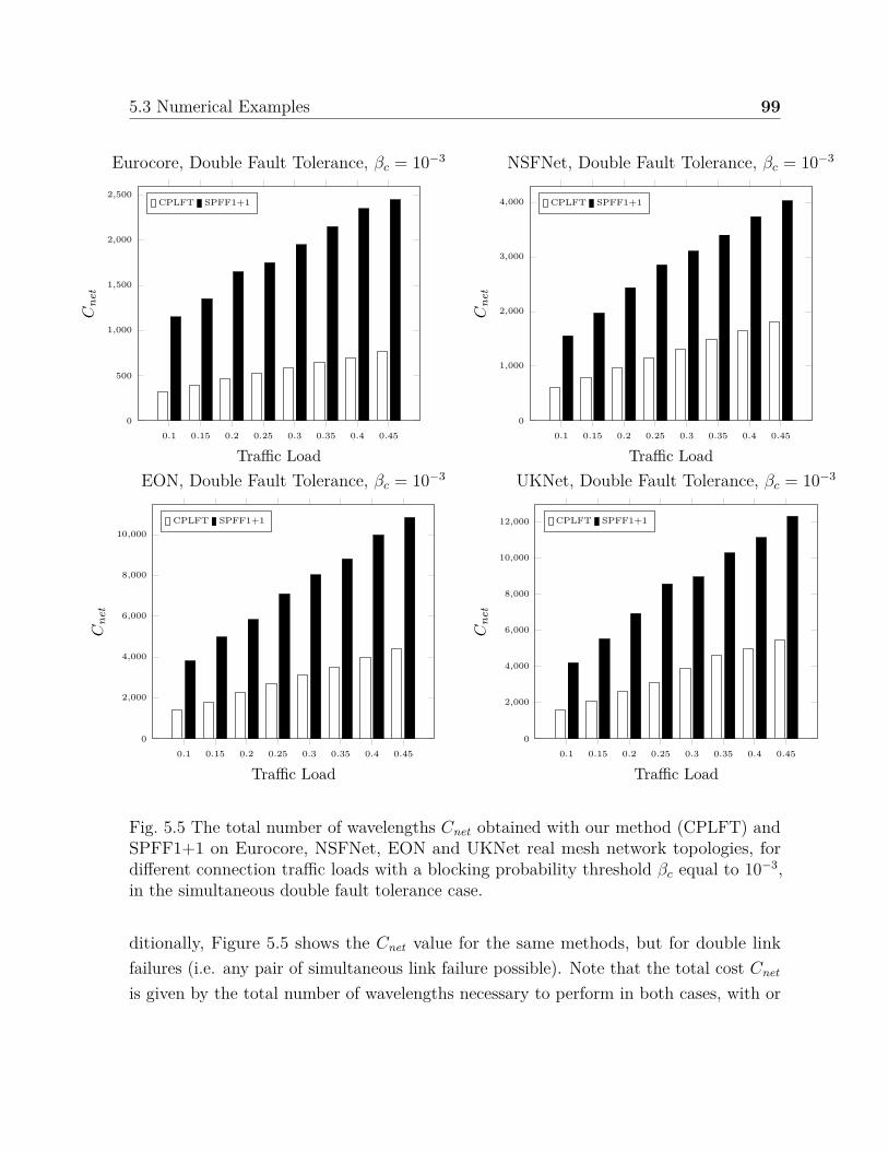
5.3 Numerical Examples 99
0.1 0.15 0.2 0.25 0.3 0.35 0.4 0.450
500
1,000
1,500
2,000
2,500
Traffic Load
Cne
t
Eurocore, Double Fault Tolerance, βc = 10−3
CPLFT SPFF1+1
0.1 0.15 0.2 0.25 0.3 0.35 0.4 0.450
1,000
2,000
3,000
4,000
Traffic LoadC
net
NSFNet, Double Fault Tolerance, βc = 10−3
CPLFT SPFF1+1
0.1 0.15 0.2 0.25 0.3 0.35 0.4 0.450
2,000
4,000
6,000
8,000
10,000
Traffic Load
Cne
t
EON, Double Fault Tolerance, βc = 10−3
CPLFT SPFF1+1
0.1 0.15 0.2 0.25 0.3 0.35 0.4 0.450
2,000
4,000
6,000
8,000
10,000
12,000
Traffic Load
Cne
tUKNet, Double Fault Tolerance, βc = 10−3
CPLFT SPFF1+1
Fig. 5.5 The total number of wavelengths Cnet obtained with our method (CPLFT) andSPFF1+1 on Eurocore, NSFNet, EON and UKNet real mesh network topologies, fordifferent connection traffic loads with a blocking probability threshold βc equal to 10−3,in the simultaneous double fault tolerance case.
ditionally, Figure 5.5 shows the Cnet value for the same methods, but for double linkfailures (i.e. any pair of simultaneous link failure possible). Note that the total cost Cnet
is given by the total number of wavelengths necessary to perform in both cases, with or
100 Fault Tolerance
without fault tolerance capability, that is, including the primary and secondary routesof every connection c (but only taking into account the actual traffic that can transmiteach possible scenario). Also, it is important to notice that in this section only singleand double link failure scenarios are shown. This is because to represent another kind offailures scenarios, such as SRG and Disaster Risk constrains, any subset selection couldbe arbitrary (not representative of a general type of failure situation). However, thealgorithm developed can easily evaluate any type of fault tolerance case.
As it can be seen in Figure 5.4, in the case of tolerance to a single failure, the CPLFTmethod performs clearly better. In fact, for all the scenarios evaluated in our experiments,the SPFF1+1 method requires in general 30% more wavelengths (for ϱ = 0.3 which is arepresentative network load [28]) than the cost of the method proposed herein. In thecase of tolerance to two simultaneous failures of links (Figure 5.5), the CPLFT methodalso significantly outperforms the SPFF1+1 technique. In this last case, the SPFF1+1method requires in the order of 160% more wavelengths (always for ϱ = 0.3 [28]) thanour proposal. Notice that each scenario presented herein achieves to connect the sameusers (connections) with the same QoS requirements (maximum acceptable blockingprobability), but our proposal requires less resources than SPFF1+1 to do so.
Now, to provide a deeper discussion of the results obtained by CPLFT, next we presentsome in details analysis about: the fault tolerance methodology used (Sub-Section5.3.1);our method memory size used and the time required to access the memory during thenetwork operation (Sub-Section5.3.2); and, finally, a general review of CPLFT method,remarking qualitative reasons that justify the better results, and some desirable featuresincluded (Sub-Section5.3.3).
5.3.1 Extra number of wavelengths
The previous analysis provides an insight of the performance of our joint solution, solvingtogether four of the most important problem in optical networks. Nevertheless, we wantto properly measure the efficiency of the solely fault tolerance procedure.
Let us define EX(A) as the extra percentage of wavelength (with respect to the nofailure case) needed to achieve fault tolerance by algorithm A. This will measure howmany extra resources are needed to provide any fault tolerance scenario, taking into

5.3 Numerical Examples 101
account each algorithm solution. The EX(A) value can be obtained as follows:
EX(A) = 100 · Cnet(A)− Cnft(A)Cnft(A) , (5.3)
where Cnft(A) is the total network cost obtained in the no failure case by the A algorithm(i.e. dimensioning the wavelengths considering only the primary routes), and Cnet as thetotal network cost evaluated by the A method on the fault tolerance case considered onthe evaluation.
In order to be fair between both methods, we define the same primary pathsand wavelength dimensioning in both methods no failure case, i.e. Cnft(CPLFT ) ≡Cnft(SPFF1 + 1). Then, to analyze each fault tolerance mechanism, Figure 5.6 containsthe EX(A) value achieve by the CPLFT and SPFF1+1 method to provide single faulttolerance on the same network topologies presented in Figure 5.3, with different meanusers traffic load for a blocking probability threshold value βc = 10−3. Similarly, Figure 5.7shows the EX(A) value on the double fault tolerance case.
The results obtained in single and double fault tolerance case shows our methodrequires to install lesser resources (wavelengths, and any equipment related to) thanSPFF1+1 solution. We strongly believe that this occurs based on two situations. First,the 1+1 mechanism guarantee certain level of fault tolerance by transmitting in parallelthe data by more than one path. This means, that on the dimensioning procedure theprimary and secondary routes are considered operational. This definitely rises the trafficon the network, leading to a bigger dimensioning than needed. Second, the homogeneousdimensioning procedure strongly relies on balancing the traffic on the network. However,as mention on chapter 4, rarely the network topologies are symmetrical, thus the networkare hard to completely balance. Therefore, the homogeneous dimensioning depends on thelink more loaded, achieving a bigger dimensioning than our heterogeneous dimensioningproposal.
5.3.2 Memory size and routing delay
Another aspects that influence the network performance are: the storage size used by therouting tables, and the delay imposed by the routing procedure when each user attemptsto transmit over a path.
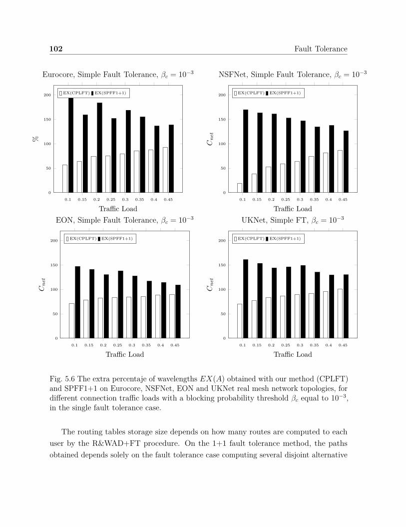
102 Fault Tolerance
0.1 0.15 0.2 0.25 0.3 0.35 0.4 0.450
50
100
150
200
Traffic Load
%
Eurocore, Simple Fault Tolerance, βc = 10−3
EX(CPLFT) EX(SPFF1+1)
0.1 0.15 0.2 0.25 0.3 0.35 0.4 0.450
50
100
150
200
Traffic LoadC
net
NSFNet, Simple Fault Tolerance, βc = 10−3
EX(CPLFT) EX(SPFF1+1)
0.1 0.15 0.2 0.25 0.3 0.35 0.4 0.450
50
100
150
200
Traffic Load
Cne
t
EON, Simple Fault Tolerance, βc = 10−3
EX(CPLFT) EX(SPFF1+1)
0.1 0.15 0.2 0.25 0.3 0.35 0.4 0.450
50
100
150
200
Traffic Load
Cne
t
UKNet, Simple FT, βc = 10−3
EX(CPLFT) EX(SPFF1+1)
Fig. 5.6 The extra percentaje of wavelengths EX(A) obtained with our method (CPLFT)and SPFF1+1 on Eurocore, NSFNet, EON and UKNet real mesh network topologies, fordifferent connection traffic loads with a blocking probability threshold βc equal to 10−3,in the single fault tolerance case.
The routing tables storage size depends on how many routes are computed to eachuser by the R&WAD+FT procedure. On the 1+1 fault tolerance method, the pathsobtained depends solely on the fault tolerance case computing several disjoint alternative

5.3 Numerical Examples 103
0.1 0.15 0.2 0.25 0.3 0.35 0.4 0.450
200
400
600
Traffic Load
%
Eurocore, Double Fault Tolerance, βc = 10−3
EX(CPLFT) EX(SPFF1+1)
0.1 0.15 0.2 0.25 0.3 0.35 0.4 0.450
200
400
600
Traffic LoadC
net
NSFNet, Double Fault Tolerance, βc = 10−3
EX(CPLFT) EX(SPFF1+1)
0.1 0.15 0.2 0.25 0.3 0.35 0.4 0.450
200
400
600
Traffic Load
Cne
t
EON, Double Fault Tolerance, βc = 10−3
EX(CPLFT) EX(SPFF1+1)
0.1 0.15 0.2 0.25 0.3 0.35 0.4 0.450
200
400
600
Traffic Load
Cne
tUKNet, Double Fault Tolerance, βc = 10−3
EX(CPLFT) EX(SPFF1+1)
Fig. 5.7 The extra percentaje of wavelengths EX(A) obtained with our method (CPLFT)and SPFF1+1 on Eurocore, NSFNet, EON and UKNet real mesh network topologies, fordifferent connection traffic loads with a blocking probability threshold βc equal to 10−3,in the simultaneous double fault tolerance case.
routes. This means, that to provide fault tolerance to a single link failure, the methodcomputes one secondary path. Likewise, to offer fault tolerance to simultaneous doublelink failure, the 1+1 technique provides two secondary routes. Therefore, the number of

104 Fault Tolerance
entries stored on the routing tables are two and three times the number of connectionsin X to provide single fault tolerance and double fault tolerance, respectively (with acentralized management).
On our method, the number of paths computed changes over the different scenariosof link failure and the network topology (size and node degree) evaluated. This is due tothe fact that on each failure case, our method searches for a new route to each connectionaffected by the failed links, computing the best possible route on that scenario. Then, thiswill provide, in general, a little more paths than the 1+1 fault tolerance method. Despitethis observation, our method requires a similar number of alternate paths to providesingle and fault tolerance than 1+1. On the Eurocore network topology to provide singleand fault tolerance, our methods computes the same number of alternate paths than 1+1.Moreover, on a bigger network such as Arpanet, our methods require on average threeand four paths to provide single and double fault tolerance, respectively.
During the network operation, there is a delay incurred by the routing procedure,defined as the time that each connection requires to find a path over the network and tosuccessfully transmit by it, or to be finally blocked. We will define this delay as τ(A),where A is the algorithm considered (SPFF1+1 or CPLFT methods). Due to the fact thatboth methods compared in this chapter use predefine routes, then the this delay is mainlycompose by the time needed to access the routing table. This value can be considered asa constant T . Then, in this context τ(A) measures the routing delay obtained by howmany times it is required to access the routing tables to have a successful communicationor to be blocked, using the routing scheme obtained by the method A.
Both methods, store the alternate paths in routing tables, but the technique to routeeach user on every communication request differs. The 1+1 fault tolerance scheme, sendsthe information on each alternate path every time the user attempts to transmit, thusthe access to routing tables requires to read each the entries including all the alternatepath, thus two routes per connection on single fault tolerance, and three routes per useron simultaneous double fault tolerance. On the other hand, our method has only oneroute per link failure case, thus CPLFT requires to read only one entry on the routingtable on each attempt of transmission.
In summary, the τ(A) value per method is:
• τ(SPFF1 + 1 ) = 2 · T , considering tolerance to single link faulure.
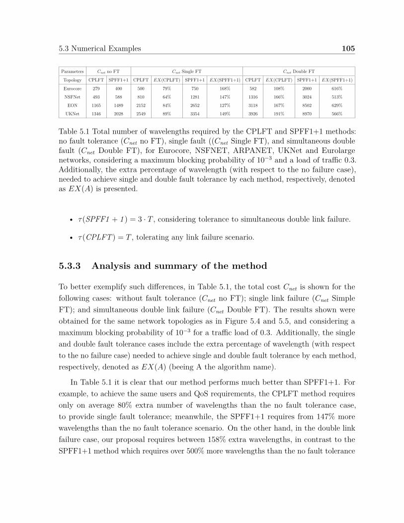
5.3 Numerical Examples 105
Parameters Cnet no FT Cnet Single FT Cnet Double FT
Topology CPLFT SPFF1+1 CPLFT EX(CPLFT) SPFF1+1 EX(SPFF1+1) CPLFT EX(CPLFT) SPFF1+1 EX(SPFF1+1)
Eurocore 279 400 500 79% 750 168% 582 108% 2000 616%
NSFNet 493 588 810 64% 1281 147% 1316 166% 3024 513%
EON 1165 1489 2152 84% 2652 127% 3118 167% 8502 629%
UKNet 1346 2028 2549 89% 3354 149% 3926 191% 8970 566%
Table 5.1 Total number of wavelengths required by the CPLFT and SPFF1+1 methods:no fault tolerance (Cnet no FT), single fault ((Cnet Single FT), and simultaneous doublefault (Cnet Double FT), for Eurocore, NSFNET, ARPANET, UKNet and Eurolargenetworks, considering a maximum blocking probability of 10−3 and a load of traffic 0.3.Additionally, the extra percentage of wavelength (with respect to the no failure case),needed to achieve single and double fault tolerance by each method, respectively, denotedas EX(A) is presented.
• τ(SPFF1 + 1 ) = 3 · T , considering tolerance to simultaneous double link failure.
• τ(CPLFT ) = T , tolerating any link failure scenario.
5.3.3 Analysis and summary of the method
To better exemplify such differences, in Table 5.1, the total cost Cnet is shown for thefollowing cases: without fault tolerance (Cnet no FT); single link failure (Cnet SimpleFT); and simultaneous double link failure (Cnet Double FT). The results shown wereobtained for the same network topologies as in Figure 5.4 and 5.5, and considering amaximum blocking probability of 10−3 for a traffic load of 0.3. Additionally, the singleand double fault tolerance cases include the extra percentage of wavelength (with respectto the no failure case) needed to achieve single and double fault tolerance by each method,respectively, denoted as EX(A) (beeing A the algorithm name).
In Table 5.1 it is clear that our method performs much better than SPFF1+1. Forexample, to achieve the same users and QoS requirements, the CPLFT method requiresonly on average 80% extra number of wavelengths than the no fault tolerance case,to provide single fault tolerance; meanwhile, the SPFF1+1 requires from 147% morewavelengths than the no fault tolerance scenario. On the other hand, in the double linkfailure case, our proposal requires between 158% extra wavelengths, in contrast to theSPFF1+1 method which requires over 500% more wavelengths than the no fault tolerance

106 Fault Tolerance
scenario requires. A notable consequence of this performance is that our method achievesdouble fault tolerance capacity with similar resources than the ones required using theSPFF1+1 method to provide just single fault tolerance.
Let us discuss here some qualitative reasons that justify the better results of CPLFTover SPFF1+1:
• By simultaneously solving the four problems (primary and secondary routing,wavelength assignment, wavelengths dimensioning and fault tolerance), a globalsolution is obtained, which is a more efficient strategy than to solve these problemsseparately.
• Our proposal allows to share the resources between the primary and secondaryroutes, just like the shared path protection, while guaranteeing certain level ofquality of service (defined on the SLA) despite the existence of any set of linkfailure, as long as the network remains connected. The latter is a characteristicsnot seen on previous methods in the literature.
• CPLFT uses a wavelength dimensioning policy without distinction between primaryand secondary routes. Therefore, it better exploits statistical multiplexing amongall requests for connection/disconnection.
• Our technique never dimensions the cases that will never happened. For example,when dimensioning a determined failure case, it does not consider the load of theprimary routes affected by the link failures. Although this fact may seem trivial,this is not considered by the 1+1 method.
• The dimensioning procedure assigns a different number of wavelengths to eachnetwork link (called Heterogeneous Dimensioning), such that the blocking probabilityof each connection does not exceed a predefined maximum blocking probability.This takes advantage that real network are hardly symmetric, thus hard to balancethe connections traffic load within.
• Additionally, the dimensioning procedure uses a wavelength assignment policy called“Fair Policy”. This policy consists in to offer a maximum blocking probability to eachnetwork user as close as possible to the one defined in the SLA, since each user mayhave different quality of service requirements. This way the method diminishes the
5.4 Conclusions 107
wavelength dimensioning since each connection uses only the wavelengths neededto satisfy their QoS demand.
• The usual blocking probability evaluation is based on simulation techniques, whichis a slow procedure. Consequently, the evaluation process is limited to only a fewrestricted scenarios. So, to find the best possible solution, researchers apply somecriteria to restrict the solutions search (heuristics). For example, using SPFF toselect the primary routes, and similar criteria to find secondary routes. However,CPLFT was able to outperform these methodologies, so we can conclude that suchheuristic solutions are not using completely accurate assumptions and decisions.We think that one of the key aspects why our proposal achieves better solutions isdue to the fact that we can quickly explore a bigger solution space to find the bestpossible solution.
In addition to the increased efficiency compared to existing methods, the CPLFTmethod has other desirable attributes:
• It is scalable to any set of simultaneous failures, as long as the network remainsconnected after those multiple failures.
• The on-line operation of the method is very fast and simple. This is due to thefact that the re-routing information is stored in routing tables, which contain thesecondary routes for each possible failure scenario. This means that the mechanismof fault tolerance can be executed quickly on demand.
• The off-line execution time of the CPLFT method takes only a few seconds using astandard current PC (Windows 10 64 bits, Intel Core i7 2.60GHz processor and8GB RAM).
5.4 Conclusions
A novel method was proposed to jointly solve four main problems in dynamic opticalnetwork design with wavelength continuity constraint: It determines the set of primaryand secondary routes using a fixed routing strategy, it defines a strategy to approachthe wavelength assignment on the network operation based on the well known First-fit

108 Fault Tolerance
scheme, it evaluates the minimum number of wavelengths necessary on each networklink so that the blocking probability of each user is lower than a certain pre-specifiedthreshold (which is a design parameter of the network), and it solves the fault toleranceproblem on any possible scenario represented as a set of possible link failures. This jointsolution allows us to obtain a global solution to these problems, which in general is betterthan to obtain them separately.
The methodology differs considerably from those published so far, obtaining betterresults in terms of necessary number of wavelengths. The method only evaluates scenariosthat happen during the network operation (for each user, it considers either a primaryor a secondary route, not both). In fact, the method allows to share the resourcesbetween the secondary routes such as Shared Path Protection methodologies, whileguaranteeing a maximum blocking probability to each network connection. Additionally,the dimensioning method does not make any distinction between primary and alternativeroutes, and it calculates a different number of wavelengths on each link (heterogeneouswavelength dimensioning). Besides, the method introduces a Fairness policy in theFirst-Fit Wavelength Assignment, in order to offer a quality of service to each user asclose as the one requested on the Service Level Agreement.
The fault tolerance technique is scalable to any set of simultaneous link failures, aslong as the network topology allows reconnection via the links that remain operating.
The method is executed before the network operation requiring a few seconds tosolve the R&WAD subtask. This allows us to quickly solve any link failure scenario andto re-evaluate in case of variations during network operation (for example, traffic loadvariations). Additionally, the network operation based on our approach is simple and fast,since the routes (both primary and secondary) are stored in routing tables and consultedonly on demand.

Chapter 6
Conclusions
6.1 General Conclusions
In this work, five of the most important problems needed to be solved where taken intoaccount in order to design dynamic WDM networks. These concern the:
• Blocking Probability evaluation.
• Routing.
• Wavelength Assignment.
• Wavelength Dimensioning.
• Fault Tolerance Capacity on any set of link failures.
There are many works in literature that propose different solutions to these problems.Usually they are solved separately, due to the fact that normally it is assumed that asimultaneous solution involves a high complexity. Thus, to diminish this difficulties itis standard to solved them as follows: first the routes are chosen; then the wavelengthassignment scheme is chosen and the amount of wavelengths available on each networklink is dimensioned; later, once solved the previous problems, the fault tolerance capacitiesare added (secondary routes and the corresponding wavelength dimensioning).
All of these problems, have to guarantee certain level of quality of service pre-established on the Service Level Agreement, measured as connection blocking probability.
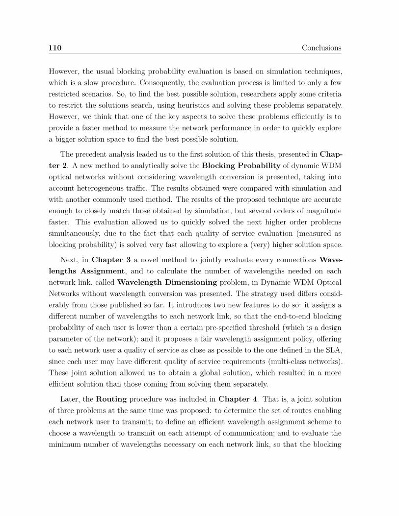
110 Conclusions
However, the usual blocking probability evaluation is based on simulation techniques,which is a slow procedure. Consequently, the evaluation process is limited to only a fewrestricted scenarios. So, to find the best possible solution, researchers apply some criteriato restrict the solutions search, using heuristics and solving these problems separately.However, we think that one of the key aspects to solve these problems efficiently is toprovide a faster method to measure the network performance in order to quickly explorea bigger solution space to find the best possible solution.
The precedent analysis leaded us to the first solution of this thesis, presented in Chap-ter 2. A new method to analytically solve the Blocking Probability of dynamic WDMoptical networks without considering wavelength conversion is presented, taking intoaccount heterogeneous traffic. The results obtained were compared with simulation andwith another commonly used method. The results of the proposed technique are accurateenough to closely match those obtained by simulation, but several orders of magnitudefaster. This evaluation allowed us to quickly solved the next higher order problemssimultaneously, due to the fact that each quality of service evaluation (measured asblocking probability) is solved very fast allowing to explore a (very) higher solution space.
Next, in Chapter 3 a novel method to jointly evaluate every connections Wave-lengths Assignment, and to calculate the number of wavelengths needed on eachnetwork link, called Wavelength Dimensioning problem, in Dynamic WDM OpticalNetworks without wavelength conversion was presented. The strategy used differs consid-erably from those published so far. It introduces two new features to do so: it assigns adifferent number of wavelengths to each network link, so that the end-to-end blockingprobability of each user is lower than a certain pre-specified threshold (which is a designparameter of the network); and it proposes a fair wavelength assignment policy, offeringto each network user a quality of service as close as possible to the one defined in the SLA,since each user may have different quality of service requirements (multi-class networks).These joint solution allowed us to obtain a global solution, which resulted in a moreefficient solution than those coming from solving them separately.
Later, the Routing procedure was included in Chapter 4. That is, a joint solutionof three problems at the same time was proposed: to determine the set of routes enablingeach network user to transmit; to define an efficient wavelength assignment scheme tochoose a wavelength to transmit on each attempt of communication; and to evaluate theminimum number of wavelengths necessary on each network link, so that the blocking

6.1 General Conclusions 111
probability of each user is lower than a certain pre-specified threshold (which is a designparameter of the network).
Finally, the Fault Tolerance was added in the procedures on Chapter 5, to jointlysolve the four technical problems presented. The routing, wavelength assignment, wave-length dimensioning, and fault tolerance capabilities on any set of link failures, whilesatisfying a predefined quality of service threshold. The method is applicable to any setof simultaneous link failures, as long as the network topology allows reconnection via thelinks that remain operating.
By relying on our analytical solution of the blocking probability proposed on Chapter 2,our proposal attempts to jointly solve the R&WAD+FT problem (presented on Figure 1.2).By doing this a global solution was obtained, which turned out to be a more efficientsolution than those coming from solving them separately.
In order to better understand each one of the solutions proposed on this thesis, nexteach chapter specific conclusions are presented.
6.1.1 Blocking probability
In Chapter 2 a new layer-based mathematical method called LIBPE for blocking prob-ability evaluation of dynamic WDM optical networks without considering wavelengthconversion and taking into account heterogeneous traffic is presented. The results obtainedhave been compared with simulation and with another commonly used method. Theresults of the proposed technique are accurate enough to closely match those obtained bysimulation.
Its main contributions are the following:
a) Our technique is that it considers that the sources are modeled by ON -OFFprocesses. This allows to take into account the non-uniform (bursty) nature of thetraffic offered to the links.
b) The link blocking dependency is handled by means of the Kelly’s Reduced Loadmethod.

112 Conclusions
c) By dividing the network into several layers, the wavelength continuity constraintcan be efficiently taken into account. The interactions between layers is consideredthrough the mean OFF periods seen on every network layer.
d) By its analytical nature, our method allows to obtain the blocking probability ofthe network in a fraction of a second. This is usually several orders of magnitudefaster than using simulation.
e) As an illustration of the calculating procedure, we report its use for wavelengthdimensioning providing a QoS guarantee on the connections’ blocking probability.By using our method, we can solve this problem 4 orders of magnitude faster thansimulation on the scenarios presented. This is relevant, because allows the networkdesigner to solve problems of higher order several times, to adjust and improve thenetwork designing procedures, to further optimize costs or benefits with respect toother parameters, etc.
6.1.2 Wavelength assignment and dimensioning
Chapter 3 presented a novel method to jointly evaluate every connections wavelengthsassignment, and to calculate the number of wavelengths needed on each network link inDynamic WDM Optical Networks without wavelength conversion.
The methodology differs considerably from those published so far. Its main contribu-tions are the following:
a) it assigns a different number of wavelengths to each network link, so that theblocking probability of each user is lower than a certain pre-specified threshold(which is a design parameter of the network).
b) it proposes a fair wavelength assignment policy, offering to each network user aquality of service as close as possible to the one defined in the SLA, since each usermay have different quality of service requirements (multi-class networks).
c) By simultaneously solving the wavelength assignment and dimensioning, a globalsolution can be obtained, which is often more efficient than a solution coming fromsolving them separately.

6.1 General Conclusions 113
d) By relying on the blocking probability method proposed in Chapter 2, the methodrequires less than a second to solve both problems. But observe that it can be usedcalling any other procedure to evaluate the blocking probability (e.g. by meansof simulation or another method available). Thus, the time required to solve thewavelength assignment and dimensioning strongly depends on the method used tocalculate this blocking probability.
6.1.3 Routing, Wavelength Assignment and Dimensioning
A new method was proposed in Chapter 4 to jointly solve three of the main problemsin optical network design. These are routing, wavelength assignment and wavelengthdimensioning.
As the previous Chapters, the strategy differs considerably from those published sofar. Its main contributions are the following:
a) Our approach jointly solves three problems at the same time: it determines the setof routes enabling each network user to transmit,it defines an efficient wavelengthassignment scheme to choose a wavelength to transmit on each attempt of commu-nication, and it evaluates the minimum number of wavelengths necessary on eachnetwork link so that the blocking probability of each user is lower than a certainpre-specified threshold (which is a design parameter of the network).
b) The features (and the benefits) presented on the previous chapter remains, due tothe fact that the this proposal uses the solution presented on Chapter 3. This are:the heterogeneous wavelength dimensioning, and the fairness policy included onthe wavelength assignment procedure.
c) By simultaneously attacking the three problems, a global solution can be obtained,which is often more efficient than that obtained when solving them separately. Thesolution is more efficient than current methods in terms of necessary number ofwavelengths.
d) The method balances the traffic load on the network, since we found out thatbalancing the network is a key aspect to diminish the amount of wavelengths whilestill guaranteeing a given level of quality of service.

114 Conclusions
e) The main work of the procedure is executed before the network is operating (off-line)and the on-line operation of our procedure is simple and fast, since the routes arestored in routing tables.
f) It requires a few seconds to solve the problem, so our approach can be adapted totraffic load variations during network operation.
6.1.4 Fault Tolerance
In Chapter 5 a novel method was proposed to jointly solve four main problems in opticalnetwork design. These concern routing, wavelength assignment, wavelength dimensioningand fault tolerance capacity on any set of link failures, so that
The methodology differs considerably from those published so far. Its main contribu-tions are the following:
a) Our approach jointly solves four problems at the same time: it determines the setof primary and secondary routes, it defines a fairness strategy to approach thewavelength assignment on the network operation, it evaluates the minimum numberof wavelengths necessary on each network link so that the blocking probability ofeach user is lower than a certain pre-specified threshold (which is a design parameterof the network), and it solves the fault tolerance problem on any possible scenariorepresented as a set of possible link failures.
b) By simultaneously attacking the four problems, a global solution can be obtained,which is often more efficient than that obtained when solving them separately. Thesolution is more efficient than current methods in terms of necessary number ofwavelengths.
c) The features (and the benefits) presented on Chapter 4 remains again, since thisproposal modifies the R&WAD strategy on Chapter 4 to provide fault tolerancecapabilities. This are: the fixed routing solution, the heterogeneous wavelengthdimensioning, and the fairness policy included on the wavelength assignment proce-dure.
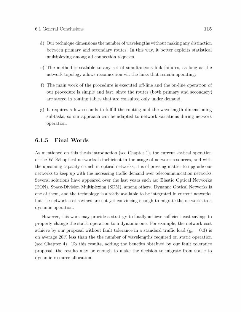
6.1 General Conclusions 115
d) Our technique dimensions the number of wavelengths without making any distinctionbetween primary and secondary routes. In this way, it better exploits statisticalmultiplexing among all connection requests.
e) The method is scalable to any set of simultaneous link failures, as long as thenetwork topology allows reconnection via the links that remain operating.
f) The main work of the procedure is executed off-line and the on-line operation ofour procedure is simple and fast, since the routes (both primary and secondary)are stored in routing tables that are consulted only under demand.
g) It requires a few seconds to fulfill the routing and the wavelength dimensioningsubtasks, so our approach can be adapted to network variations during networkoperation.
6.1.5 Final Words
As mentioned on this thesis introduction (see Chapter 1), the current statical operationof the WDM optical networks is inefficient in the usage of network resources, and withthe upcoming capacity crunch in optical networks, it is of pressing matter to upgrade ournetworks to keep up with the increasing traffic demand over telecommunication networks.Several solutions have appeared over the last years such as: Elastic Optical Networks(EON), Space-Division Multiplexing (SDM), among others. Dynamic Optical Networks isone of them, and the technology is already available to be integrated in current networks,but the network cost savings are not yet convincing enough to migrate the networks to adynamic operation.
However, this work may provide a strategy to finally achieve sufficient cost savings toproperly change the static operation to a dynamic one. For example, the network costachieve by our proposal without fault tolerance in a standard traffic load (ϱc = 0.3) ison average 20% less than the the number of wavelengths required on static operation(see Chapter 4). To this results, adding the benefits obtained by our fault toleranceproposal, the results may be enough to make the decision to migrate from static todynamic resource allocation.


References
[1] Andrew R. Chraplyvy. Plenary paper: The coming capacity crunch. In 2009 35thEuropean Conference on Optical Communication, page 8007, 2009.
[2] David J Richardson. Applied physics. Filling the light pipe. Science (New York,N.Y.), 330(6002):327–328, 2010.
[3] Dirk van den Borne, Mohammad S. Alfiad, and Sander L. Jansen. The CapacityCrunch Challenge: How to Design the Next Generation of Ultra-High CapacityTransmission Systems - OSA Technical Digest (CD). In SPPCom - Signal Processingin Photonic Communications - OSA Technical Digest, page SPTuA1, 2010.
[4] A. D. Ellis, N. Mac Suibhne, D. Saad, and D. N. Payne. Communication networksbeyond the capacity crunch. Philosophical Transactions of the Royal Society A:Mathematical, Physical and Engineering Sciences, 374(2062):20150191, 2016.
[5] Alejandra Zapata-Beghelli and Polina Bayvel. Dynamic Versus Static Wavelength-Routed Optical Networks. Lightwave Technology, Journal of, 26(20):3403–3415, oct2008.
[6] Ahmed Mokhtar and Murat Azizo\uglu. Adaptive Wavelength Routing in All-opticalNetworks. IEEE/ACM Trans. Netw., 6(2):197–206, 1998.
[7] Biswanath Mukherjee. Optical WDM networks, volume 26. Springer Science &Business Media, 2006.
[8] Michael Düser, Alejandra Zapata, and Polina Bayvel. Investigation of the scalabilityof dynamic wavelength-routed optical networks \[Invited\]. J. Opt. Netw., 3(9):674–693, sep 2004.
[9] Rajiv Ramaswami, Kumar Sivarajan, and Galen Sasaki. Optical Networks: APractical Perspective, 3rd Edition. Morgan Kaufmann Publishers Inc., San Francisco,CA, USA, 3rd edition, 2009.
[10] Hui Zang, Jason P Jue, Biswanath Mukherjee, and Others. A review of routingand wavelength assignment approaches for wavelength-routed optical WDMnetworks. Optical Networks Magazine, 1(1):47–60, 2000.
118 References
[11] Bijoy Chand Chatterjee, Nityananda Sarma, and Partha Pratim Sahu. Reviewand Performance Analysis on Routing and Wavelength Assignment Approaches forOptical Networks. IETE Technical Review, 30(1):12–23, 2013.
[12] Ravi Teja Koganti and Deepinder Sidhu. Analysis of routing and wavelengthassignment in large WDM networks. In Procedia Computer Science, volume 34,pages 71–78, 2014.
[13] Asuman E. Ozdaglar and Dimitri P. Bertsekas. Routing and wavelength assignmentin optical networks. IEEE/ACM Transactions on Networking, 11(2):259–272, 2003.
[14] S Subramaniam and R A Barry. Wavelength assignment in fixed routing WDMnetworks. Communications, 1997. ICC 97 Montreal, ’Towards the KnowledgeMillennium’. 1997 IEEE International Conference on, 1:406 –410 vol.1, 1997.
[15] Dhritiman Banerjee and Biswanath Mukherjee. A practical approach for routingand wavelength assignment in large wavelength-routed optical networks. IEEEJournal on Selected Areas in Communications, 14(5):903–908, 1996.
[16] I Chlamtac, A Ganz, and G Karmi. Lightpath communications: an approach to highbandwidth optical WAN’s. Communications, IEEE Transactions on, 40(7):1171–1182, jul 1992.
[17] X. Sun, Y. Li, I. Lambadaris, and Y.Q. Zhao. Performance analysis of first-fitwavelength assignment algorithm in optical networks. In Proceedings of the 7thInternational Conference on Telecommunications, 2003. ConTEL 2003., volume 2,pages 403–409 vol.2, 2003.
[18] Dhritiman Banerjee and Biswanath Mukherjee. Wavelength-routed optical networks:Linear formulation, resource budgeting tradeoffs, and a reconfiguration study.IEEE/ACM Transactions on Networking, 8(5):598–607, 2000.
[19] Liying Tan, Qinglong Yang, Jing Ma, and Shiqi Jiang. Wavelength Dimensioningof Optical Transport Networks Over Nongeosychronous Satellite Constellations.Journal of Optical Communications and Networking, 2(4):166–174, 2010.
[20] A L Chiu, G Choudhury, G Clapp, R Doverspike, J W Gannett, J G Klincewicz,G Li, R A Skoog, J Strand, A Von Lehmen, and D Xu. Network Design andArchitectures for Highly Dynamic Next-Generation IP-Over-Optical Long DistanceNetworks. Journal of Lightwave Technology, 27(12):1878–1890, 2009.
[21] Maurice Gagnaire, Mohamed Koubàa, and Nicolas Puech. Network dimensioningunder scheduled and random lightpath demands in all-optical WDM networks.IEEE Journal on Selected Areas in Communications, 25(9):58–67, 2007.
[22] Jing Teng and George N Rouskas. Routing path optimization in optical burstswitched networks. In Proc. ONDM, volume 2005. Citeseer, 2005.

References 119
[23] Jintae Yu, I Yamashita, S Seikai, and K Kitayama. Upgrade design of survivablewavelength-routed networks for increase of traffic loads. In Conference onOpticalNetwork Design and Modeling, 2005., pages 163–174, feb 2005.
[24] E Kozlovski, M Duser, I De Miguel, and P Bayvel. Analysis of burst scheduling fordynamic wavelength assignment in optical burst-switched networks. In IEEE, Proc.LEOS, volume 1, 2001.
[25] Wouter Van Parys, Bart Van Caenegem, and Piet Demeester. Reduction of blockingin arbitrary meshed WDM networks through a biased routing approach. In OpticalFiber Communication Conference and Exhibit, 1998. OFC’98., Technical Digest,page 94. IEEE, 1998.
[26] Gerald R Ash. Dynamic Routing in Telecommunications Networks. McGraw-HillProfessional, 1st edition, 1997.
[27] Srinivasan Keshav. An engineering approach to computer networking: ATMnetworks, the Internet, and the telephone network. Reading MA, 11997, 1997.
[28] A A M Saleh and Jane M Simmons. Technology and architecture to enable theexplosive growth of the internet. Communications Magazine, IEEE, 49(1):126–132,2011.
[29] M To and P Neusy. Unavailability analysis of long-haul networks. Selected Areasin Communications, IEEE Journal on, 12(1):100–109, 1994.
[30] D A Schupke, A Autenrieth, and T Fischer. Survivability of Multiple Fiber DuctFailures. In Third International Workshop on the Design of Reliable CommunicationNetworks (DRCN, pages 7–10, 2001.
[31] S. J B Yoo. Wavelength conversion technologies for WDM network applications.Journal of Lightwave Technology, 14(6):955–966, 1996.
[32] Byrav Ramamurthy and Biswanath Mukherjee. Wavelength conversion in WDMnetworking. IEEE Journal on Selected Areas in Communications, 16(7):1061–1073,1998.
[33] Ioannis Tomkos, Marianna Angelou, RamónJ. Durán Barroso, Ignacio de Miguel,RubénM. Lorenzo Toledo, Domenico Siracusa, Elio Salvadori, Andrzej Tymecki,Yabin Ye, and Idelfonso Tafur Monroy. Next Generation Flexible and CognitiveHeterogeneous Optical Networks. In Federico Alvarez, Frances Cleary, Petros Daras,John Domingue, Alex Galis, Ana Garcia, Anastasius Gavras, Stamatis Karnourskos,Srdjan Krco, Man-Sze Li, Volkmar Lotz, Henning Müller, Elio Salvadori, Anne-Marie Sassen, Hans Schaffers, Burkhard Stiller, Georgios Tselentis, Petra Turkama,and Theodore Zahariadis, editors, The Future Internet, volume 7281 of LectureNotes in Computer Science, pages 225–236. Springer Berlin Heidelberg, 2012.
[34] O Gerstel, M Jinno, A Lord, and S J B Yoo. Elastic optical networking: a newdawn for the optical layer? Communications Magazine, IEEE, 50(2):s12–s20, 2012.
120 References
[35] N Sambo, Piero Castoldi, F Cugini, G Bottari, and P Iovanna. Toward high-rateand flexible optical networks. Communications Magazine, IEEE, 50(5):66–72, may2012.
[36] I T Monroy, D Zibar, N G Gonzalez, and R Borkowski. Cognitive HeterogeneousReconfigurable Optical Networks (CHRON): Enabling technologies and techniques.In Transparent Optical Networks (ICTON), 2011 13th International Conference on,pages 1–4, 2011.
[37] D. J. Richardson, J. M. Fini, and L. E. Nelson. Space-division multiplexing inoptical fibres. Nature Photonics, 7(5):354–362, 2013.
[38] Dan M. Marom and Miri Blau. Switching solutions for WDM-SDM optical networks.IEEE Communications Magazine, 53(2):60–68, 2015.
[39] M. Jinno, H. Takara, and B. Kozicki. Dynamic optical mesh networks: Drivers,challenges and solutions for the future. 2009 35th European Conference on OpticalCommunication, pages 2–5, 2009.
[40] Reinaldo Vallejos, Alejandra Zapata, and Marco Aravena. Fast and effective dimen-sioning algorithm for end-to-end optical burst switching networks with ON-OFF traffic model. In Optical Network Design and Modeling, pages 378–387.Springer, 2007.
[41] R. Vallejos and N. Jara. Join routing and dimensioning heuristic for dynamic WDMoptical mesh networks with wavelength conversion. Optical Fiber Technology, 20(3),2014.
[42] S. Ramamurthy and Biswanath Mukherjee. Survivable WDM mesh networks, PartI - Protection. In Proceedings - IEEE INFOCOM, volume 2, pages 744–751, 1999.
[43] S. Chalasani and V. Rajaravivarma. Survivability in optical networks. In SystemTheory, 2003. Proceedings of the 35th Southeastern Symposium on, volume 2003-Janua, pages 6–10, 2003.
[44] A Sano, T Kobayashi, S Yamanaka, A Matsuura, H Kawakami, Y Miyamoto,K Ishihara, and H Masuda. 102.3-Tb/s (224 x 548-Gb/s) C- and extended L-bandall-Raman transmission over 240 km using PDM-64QAM single carrier FDM withdigital pilot tone. In Optical Fiber Communication Conference and Exposition(OFC/NFOEC), 2012 and the National Fiber Optic Engineers Conference, pages1–3, 2012.
[45] Anwar Alyatama. Computing blocking probabilities in survivable WDM opticalnetworks. Photonic Network Communications, 27(1):34–46, 2014.
[46] Anwar Alyatama. Wavelength Decomposition Approach for Computing BlockingProbabilities in Multicast WDM Optical Networks. Opt. Switch. Netw., 12:24–33,2014.

References 121
[47] Joan Triay, Cristina Cervelló-Pastor, and Vinod M Vokkarane. Analytical BlockingProbability Model for Hybrid Immediate and Advance Reservations in OpticalWDM Networks. IEEE/ACM Trans. Netw., 21(6):1890–1903, 2013.
[48] V Abramov, Shuo Li, Meiqian Wang, E W M Wong, and M Zukerman. Computationof Blocking Probability for Large Circuit Switched Networks. CommunicationsLetters, IEEE, 16(11):1892–1895, 2012.
[49] Jun He, Maïté Brandt-Pearce, and Suresh Subramaniam. Analysis of BlockingProbability for First-Fit Wavelength Assignment in Transmission-Impaired OpticalNetworks. J. Opt. Commun. Netw., 3(5):411–425, may 2011.
[50] Anwar Alyatama. Wavelength decomposition approach for computing blockingprobabilities in WDM optical networks without wavelength conversions. ComputerNetworks, 49(6):727–742, 2005.
[51] Kejie Lu, Gaoxi Xiao, and I Chlamtac. Analysis of blocking probability fordistributed lightpath establishment in WDM optical networks. Networking,IEEE/ACM Transactions on, 13(1):187–197, feb 2005.
[52] Ashwin Sridharan and K N Sivarajan. Blocking in all-optical networks. Networking,IEEE/ACM Transactions on, 12(2):384–397, 2004.
[53] R. Vallejos, J. Olavarría, and N. Jara. Blocking evaluation and analysis of dynamicWDM networks under heterogeneous ON/OFF traffic. Optical Switching andNetworking, 20, 2016.
[54] Luiz H Bonani and Iguatemi E Fonseca. Estimating the blocking probability inwavelength-routed optical networks. Optical Switching and Networking, 10(4):430–438, 2013.
[55] Yongli Zhao and Jie Zhang. Blocking probability analysis model for flexible spectrumoptical networks. Chin. Opt. Lett., 12(7):70601, jul 2014.
[56] R C Almeida, D R Campelo, H Waldman, and K Guild. Accounting for linkload correlation in the estimation of blocking probabilities in arbitrary networktopologies. Communications Letters, IEEE, 11(7):625–627, 2007.
[57] B Iversen Villy. Teletraffic Engineering Handbook, 2002.
[58] A A Fredericks. Congestion in Blocking Systems—A Simple Approximation Tech-nique. Bell System Technical Journal, 59(6):805–827, 1980.
[59] Thomas Bonald. The Erlang Model with Non-poisson Call Arrivals. SIGMETRICSPerform. Eval. Rev., 34(1):276–286, 2006.
[60] Jianan Zhang, Yu Peng, Eric W M Wong, and Moshe Zukerman. Sensitivity ofblocking probability in the generalized Engset model for OBS. CommunicationsLetters, IEEE, 15(11):1243–1245, 2011.

122 References
[61] Sheldon Ross. Stochastic Processes. John Wiley & Sons, Inc., 2nd edition, 1996.
[62] Qian Chen, Gurusamy Mohan, and Kee Chaing Chua. Route optimization in opticalburst switched networks considering the streamline effect. Computer Networks,52(10):2033–2044, 2008.
[63] F P Kelly. Loss Networks. The Annals of Applied Probability, 1(3):pp. 319–378,1991.
[64] An Ge, Franco Callegati, and Lakshman S Tamil. On optical burst switching andself-similar traffic. Communications Letters, IEEE, 4(3):98–100, 2000.
[65] Yijun Xiong, Marc Vandenhoute, and Hakki C Cankaya. Control architecture inoptical burst-switched WDM networks. Selected Areas in Communications, IEEEJournal on, 18(10):1838–1851, 2000.
[66] T K Nayak and K N Sivarajan. A new approach to dimensioning optical networks.IEEE Journal on Selected Areas in Communications, 20(1):134–148, 2002.
[67] I. Chlamtac, A. Ganz, and G. Karmi. Purely optical networks for terabit communi-cation. In Proceedings - IEEE INFOCOM, pages 887–896, 1989.
[68] Jun Zheng and Hussein T. Mouftah. Routing and wavelength assignment for advancereservation in wavelength-routed WDM optical networks. IEEE InternationalConference on Communications, 5:2722–2726, 2002.
[69] D R Hjelme, A Royset, and B J Slagsvold. How many wavelengths does it take tobuild a wavelength routed optical network? In Proceedings of European Conferenceon Optical Communication, volume 1, pages 27–30 vol.1, sep 1996.
[70] Stefano Baroni and Polina Bayvel. Wavelength requirements in arbitrarily connectedwavelength-routed optical networks. Journal of Lightwave Technology, 15(2):242–251, feb 1997.
[71] O Gerstel and S Kutten. Dynamic wavelength allocation in all-optical ring networks.In Communications, 1997. ICC ’97 Montreal, Towards the Knowledge Millennium.1997 IEEE International Conference on, volume 1, pages 432–436 vol.1, jun 1997.
[72] Giancarlo Marchis and Roberto Sabella, editors. Optical Networks: Design andModelling. Springer US, Boston, MA, 1 edition, 1999.
[73] J. Li, G. Mohan, and K.C. Chua. Dynamic load balancing in IP-over-WDM opticalburst switching networks. Computer Networks, 47(3):393–408, 2005.
[74] Mauro Brunato, Roberto Battiti, and Elio Salvadori. Dynamic Load Balancing inWDM Networks, 2003.
[75] Wanjiun Liao and Chi Hong Loi. Providing service differentiation for optical-burst-switched networks. Journal of Lightwave Technology, 22(7):1651–1660, 2004.
References 123
[76] Chi-Hong Loi Chi-Hong Loi, Wanjiun Liao Wanjiun Liao, and De-Nian YangDe-Nian Yang. Service differentiation in optical burst switched networks. GlobalTelecommunications Conference 2002 GLOBECOM 02 IEEE, 3, 2002.
[77] Yang Chen Yang Chen, M Hamdi, and D H K Tsang. Proportional QoS overOBS networks. GLOBECOM01 IEEE Global Telecommunications Conference CatNo01CH37270, 3:1510 –1514 vol.3, 2001.
[78] Nail Akar, Ezhan Karasan, Kyriakos G. Vlachos, Emmanouel A. Varvarigos, DavideCareglio, Miroslaw Klinkowski, and Josep Solé-Pareta. A survey of quality of servicedifferentiation mechanisms for optical burst switching networks, 2010.
[79] Li Yang and George N. Rouskas. Optimal wavelength sharing policies in OBSnetworks subject to QoS constraints. IEEE Journal on Selected Areas in Commu-nications, 25(9):40–49, 2007.
[80] Li Yang and George N. Rouskas. Generalized wavelength sharing policies forabsolute QoS guarantees in OBS networks. IEEE Journal on Selected Areas inCommunications, 25(4):93–103, 2007.
[81] Nicolás Jara, Reinaldo Vallejos, and Gerardo Rubino. Blocking Evaluation andWavelength Dimensioning of Dynamic WDM Networks Without Wavelength Con-version. Journal of Optical Communications and Networking, 9(8):625, 2017.
[82] N Jara, R Vallejos, and G Rubino. Blocking evaluation of dynamic WDM networkswithout wavelength conversion. In 2016 21st European Conference on Networksand Optical Communications (NOC), pages 141–146, 2016.
[83] Reinaldo Jara, Nicolas; Rubino, Gerardo; Vallejos. Blocking Evaluation of dynamicWDM networks without wavelength conversion. In 11ème Atelier en Evaluation dePerformances, Toulouse, France, 2016.
[84] Sungchang Kim, Jin Seek Choi, and Minho Kang. Absolute Differentiated Servicesfor Optical Burst Switching Networks Using Dynamic Wavelength Assignment. InSPIE Multimedia Computing and Networking, pages 855–866, 2004.
[85] Jun Zheng, Baoxian Zhang, and Hussein T. Mouftah. Toward automated provi-sioning of advance reservation service in next-generation optical Internet. IEEECommunications Magazine, 44(12):68–74, 2006.
[86] Neal Charbonneau and Vinod M. Vokkarane. A survey of advance reservationrouting and wavelength assignment in wavelength-routed WDM networks. IEEECommunications Surveys and Tutorials, 14(4):1037–1064, 2012.
[87] C Meza, N Jara, V M Albornoz, and R Vallejos. Routing and spectrum assignmentfor elastic, static, and without conversion optical networks with ring topology.In 2016 35th International Conference of the Chilean Computer Science Society(SCCC), pages 1–8, oct 2016.
124 References
[88] Jing Teng and George Rouskas. Traffic engineering approach to path selection inoptical burst switching networks. J. Opt. Netw., 4(11):759–777, nov 2005.
[89] Jin Y. Yen. Finding the <i>K</i> Shortest Loopless Paths in a Network. Man-agement Science, 17(11):712–716, 1971.
[90] Reinaldo Vallejos, Alejandra Zapata-Beghelli, V\’\ictor Albornoz, and MarcoTarifeño. Joint routing and dimensioning of optical burst switching networks.Photonic Network Communications, 17(3):266–276, 2009.
[91] R Ramaswami and K N Sivarajan. Design of logical topologies for wavelength-routedall-optical networks. In INFOCOM ’95. Fourteenth Annual Joint Conference of theIEEE Computer and Communications Societies. Bringing Information to People.Proceedings. IEEE, pages 1316–1325 vol.3, 1995.
[92] Hardeep Singh, Jai Prakash, Dinesh Arora, and Amit Wason. Fault TolerantCongestion Based Algorithms in OBS Network. International Journal ofEngineering (IJE), 5(5), 2011.
[93] Fernanda Sumika H Souza, Daniel L Guidoni, and Geraldo R Mateus. A columngeneration-based heuristic for the GRWA with protection and QoS in WDM opticalnetworks. In Computers and Communications (ISCC), 2013 IEEE Symposium on,pages 922–927, 2013.
[94] D S Mukherjee, C Assi, and A Agarwal. Alternate Strategies for Dual FailureRestoration Using p-Cycles. In Communications, 2006. ICC ’06. IEEE InternationalConference on, volume 6, pages 2477–2482, 2006.
[95] Raghav Yadav, RamaShankar Yadav, and HariMohan Singh. Intercycle switching(ICS)-based dynamic reconfiguration of p-cycle for dual-failure survivability ofWDM networks. Photonic Network Communications, 24(2):160–165, 2012.
[96] Liangrui Tang, Mingming Cai, Bin Li, and Runze Wu. A novel multi-link fault-tolerant algorithm for survivability in multi-domain optical networks. PhotonicNetwork Communications, 24(2):77–85, 2012.
[97] Dharmendra Singh Yadav, Santosh Rana, and Shashi Prakash. A mixed connectionrecovery strategy for surviving dual link failure in WDM networks. Optical FiberTechnology, 19(2):154–161, 2013.
[98] Ferhat Dikbiyik, Abu S Reaz, Marc De Leenheer, and Biswanath Mukherjee. Mini-mizing the disaster risk in optical telecom networks. In Optical Fiber CommunicationConference, pages OTh4B—-2. Optical Society of America, 2012.
[99] Sifat Ferdousi, Ferhat Dikhiyik, M Farhan Habib, and Biswanath Mukherjee.Disaster-aware data-center and content placement in cloud networks. In 2013 IEEEInternational Conference on Advanced Networks and Telecommunications Systems(ANTS), pages 1–3. IEEE, 2013.

References 125
[100] Hui Zang, Canhui Ou, and Biswanath Mukherjee. Path-protection routing andwavelength assignment in WDM mesh networks under shared-risk-group constraints.In Asia-Pacific Optical and Wireless Communications Conference and Exhibit,pages 49–60. International Society for Optics and Photonics, 2001.
[101] S Ramamurthy, L Sahasrabuddhe, and B Mukherjee. Survivable WDM meshnetworks. Lightwave Technology, Journal of, 21(4):870–883, 2003.
[102] G Mohan and C S R Murthy. Lightpath restoration in WDM optical networks.Network, IEEE, 14(6):24–32, nov 2000.
[103] P C Srikanth, M V Sathyanarayana, D Balaraju, and T Srinivas. Fault tolerancein survivable WDM optical networks using hybrid scheme: An analytical approach.In TENCON 2009 - 2009 IEEE Region 10 Conference, pages 1–6, 2009.
[104] M Wang, S Li, E W M Wong, and M Zukerman. Performance Analysis of CircuitSwitched Multi-Service Multi-Rate Networks With Alternative Routing. Journalof Lightwave Technology, 32(2):179–200, 2014.
[105] DominicA. Schupke and RobertG. Prinz. Capacity Efficiency and Restorabilityof Path Protection and Rerouting in WDM Networks Subject to Dual Failures.Photonic Network Communications, 8(2):191–207, 2004.
[106] Jing Zhang and B Mukheriee. A review of fault management in WDM meshnetworks: basic concepts and research challenges. Network, IEEE, 18(2):41–48, mar2004.
[107] Amit Wason and R S Kaler. Fault-tolerant routing and wavelength assignment algo-rithm for multiple link failures in wavelength-routed all-optical WDM networks.Optik - International Journal for Light and Electron Optics, 122(2):110–113, 2011.
[108] D A Schupke, C G Gruber, and A Autenrieth. Optimal Configuration of p-Cyclesin WDM Networks. In In IEEE International Conference on Communications,pages 2761–2765, 2002.
[109] D A Schupke. Multiple failure survivability in WDM networks with p-cycles. InCircuits and Systems, 2003. ISCAS ’03. Proceedings of the 2003 InternationalSymposium on, volume 3, pages III–866–III–869 vol.3, may 2003.
[110] D A Schupke, W D Grover, and M Clouqueur. Strategies for enhanced dual failurerestorability with static or reconfigurable p-cycle networks. In Communications,2004 IEEE International Conference on, volume 3, pages 1628–1633, 2004.
[111] Mirosław Klinkowski, João Pedro, Davide Careglio, Michał Pióro, João Pires, PauloMonteiro, and Josep Solé-Pareta. An overview of routing methods in optical burstswitching networks. Optical Switching and Networking, 7(2):41–53, 2010.
[112] C Yahaya, Abd Latiff, and A B Mohamed. A review of routing strategies for opticalburst switched networks. International Journal of Communication Systems, 2011.

126 References
[113] Erick Donato, Joaquim Celestino Júnior, Antônio Vieira, and Ahmed Patel. AProposal of Dynamic RWA Using Ant Colony in Optical Burst Switched Networks.In ICN 2012, The Eleventh International Conference on Networks, pages 246–252,2012.
[114] Dewiani, K Hirata, Y Higami, and S.-Y. Kobayashi. Dynamic routing and wave-length assignment in multifiber WDM networks with sparse wavelengthconversion. In ICT Convergence (ICTC), 2012 International Conference on, pages567–572, 2012.
[115] Lucile Belgacem, Irène Charon, and Olivier Hudry. A post-optimization methodfor the routing and wavelength assignment problem applied to scheduled lightpathdemands. European Journal of Operational Research, 2013.
[116] Amin Ebrahimzadeh, Akbar Ghaffarpour Rahbar, and Behrooz Alizadeh. Binaryquadratic programming formulation for routing and wavelength assignment problemin all-optical WDM networks. Optical Switching and Networking, 10(4):354–365, 2013.
[117] Chia-Chun Hsu, Hsun-Jung Cho, and Shu-Cherng Fang. Routing and WavelengthAssignment in Optical Networks from Maximum Edge-Disjoint Paths. In Geneticand Evolutionary Computing, volume 238 of Advances in Intelligent Systems andComputing, pages 95–103. Springer International Publishing, 2014.
[118] Nicolás Jara, Reinaldo Vallejos, and Gerardo Rubino. A method for joint routing,wavelength dimensioning and fault tolerance for any set of simultaneous failures ondynamic WDM optical networks. Optical Fiber Technology, 38:30–40, 2017.
[119] N. Jara, G. Rubino, and R. Vallejos. Alternate paths for multiple fault toleranceon Dynamic WDM Optical Networks. In IEEE International Conference on HighPerformance Switching and Routing, HPSR, volume 2017-June, 2017.

Titre : Conception de réseaux optiques en tenant compte de la tolérance aux fautes d’un ensemble quelconque de liens
Mots clés : réseaux optiques dynamiques, probabilité de blocage, tolérance aux fautes
Résumé : L’augmentation rapide de la demande en bande passante dans les réseaux de télécommunication d’aujourd’hui a provoqué une augmentation correspondante de l’utilisation de technologies basées dans les réseaux optiques de type WDM. Ceci étant, la recherche a identifié une limite forte dans la capacité de croissance de ces infrastructures, du point de la vitesse de transmission, limite qui sera atteinte bientôt. Cette situation conduit à des efforts de recherche pour faire évoluer les architectures courantes vers de nouvelles solutions capables d’absorber cette croissance dans la demande. Par exemple, les réseaux d’aujourd’hui sont opérés de façon statique. Ceci est inefficace dans l’utilisation des ressources, et la nécessité d’améliorer cet état de fait est reconnue par la recherche ainsi que par l’industrie. Plusieurs solutions ont été proposées pour passer à des modes de fonctionnement dynamiques, mais les diminutions des coûts qu’ont été obtenues n’ont pas encore convaincu les industriels.
Cette thèse fait une nouvelle proposition de cette nature, qui inclut une nouvelle et très rapide méthodologie pour évaluer la probabilité de blocage dans ce type de système, qui est le cœur de notre procédure de conception. Le travail réalisé a conduit à la découverte de solutions pour l’ensemble des problèmes principaux d’une architecture de transmission optique. Il s’agit de décider chemins à utiliser par chaque utilisateur et la longueur d’onde (Wavelength Assignment Problem). Ensuite, il faut choisir le nombre total de longueurs d’onde qui sera nécessaire (Wavelength Dimensioning Problem). Enfin, il faut proposer les procédures à suivre en cas de défaillance d’un ou de plusieurs liens du réseau (Fault Tolerance Problem). La thèse propose une solution globale à cet ensemble de problèmes, et montre que les gains que l’on peut espérer dans l’opération de ces réseaux sont significativement plus importants qu’avec les autres propositions existantes.
Title : Optical Network Design considering Fault Tolerance to any set of link failures
Keywords : optical netowrks, blocking probability, fault tolerance
Abstract : The rapid increase in demand for bandwidth from existing networks has caused a growth in the use of technologies based on WDM optical networks. Nevertheless, this decade researchers have recognized a “Capacity Crunch” on optical networks, i.e. transmission capacity limit on optical fiber is close to be reached in the near future. This situation claims to evolve the current WDM optical networks architectures. For example, optical networks are operated statically. This operation is inefficient in the usage of network resources. To solve this problem Dynamic optical networks solve this inefficiences, but it has not been implemented since network cost savings are not enough to convince enterprises. The design of dynamic optical networks decomposes into different tasks, where the engineers must organize the way the main system’s resources are used.
All of these tasks, have to guarantee certain level of quality of service pre-established on the Service Level Agreement. Then, we propose a new fast and accurate analytical method to evaluate the blocking probability in these systems. This evaluation allows network designers to quickly solve higher order problems. More specifically, network operators face the challenge of solving: which wavelength is going to be used by each user (known as Wavelength Assignment), the number of wavelengths needed on each network link (called as Wavelength Dimensioning), the set of paths enabling each network user to transmit (known as Routing) and how to deal with link failures when the network is operating (called as Fault Tolerance capacity). This thesis proposes a joint solution to these problems, and it may provide sufficient network cost savings to foster telecommunications companies to migrate from the current static operation to a dynamic one.