![[O. Svelto, D. Hanna] Principles of Lasers(BookZZ.org)](https://static.fdocuments.in/doc/165x107/55cf9702550346d0338f3fe2/o-svelto-d-hanna-principles-of-lasersbookzzorg.jpg)
“Optical Measurements” - Intranet...
42
1/38 Alignment/Pointing and Dimensional Measurements Prof. Cesare Svelto Politecnico di Milano Some pictures are taken from the Book “Electro-Optical Instrumentation: Sensing and Measuring with Lasers” by Prof. Silvano Donati “Optical Measurements” Master Degree in Engineering Automation-, Electronics-, Physics-, Telecommunication- Engineering
Transcript of “Optical Measurements” - Intranet...

1/38
Alignment/Pointing and
Dimensional Measurements
Prof. Cesare SveltoPolitecnico di Milano
Some pictures are taken from the Book “Electro-Optical Instrumentation: Sensing and Measuring with Lasers” by Prof. Silvano Donati
“Optical Measurements”Master Degree in EngineeringAutomation-, Electronics-, Physics-, Telecommunication- Engineering
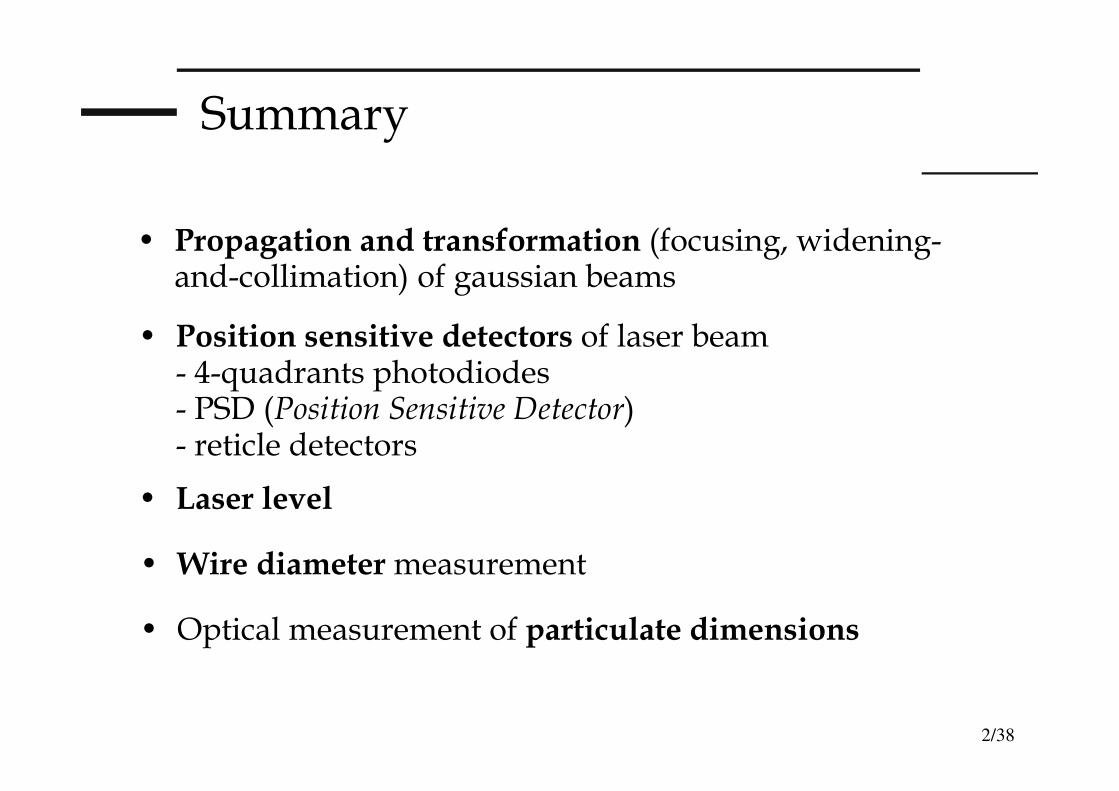
2/38
Summary
• Propagation and transformation (focusing, widening-and-collimation) of gaussian beams
• Position sensitive detectors of laser beam- 4-quadrants photodiodes- PSD (Position Sensitive Detector)- reticle detectors
• Laser level
• Wire diameter measurement
• Optical measurement of particulate dimensions

3/38
Laser alignment
One property of laser sources is the possibility of keeping the optical bem well collimated (slightly divergent and hence with “constant spot size" during propagation)
The divergence limit posed by diffraction theory (TEM00)is “easy to meet”: e.g. for an He-Ne LASER (633 nm).Visible light is useful for alignment in a specific direction("filo a piombo" not only vertical)
We must minimize the laser spot dimension on the whole working region (range ±z*) and to this aim we must design an optimal value of the beam waist (w0) in the center of the range: for this purpose we use a telescope to “widen the spot size to the desired dimension"

4/38
Laser alignment in constructions
Typical instrument for laser alignment andits use in the construction of gas pipeline(LaserLight AG, Munich)

5/38
Propagation of a laser Gaussian beam
Divergence of the laser spot (free space)
Output beam from a laser (e.g. He-Ne)with plane-spherical cavity
ROCbeam waist in theplane-spherical resonator
it mustbeL≤ROC
r=∞∞∞∞ ot z=0 and at z=∞∞∞∞ (plane wave)minimum rMIN=2zR at z=zR
Curvature Radiusof the wave front
6/38
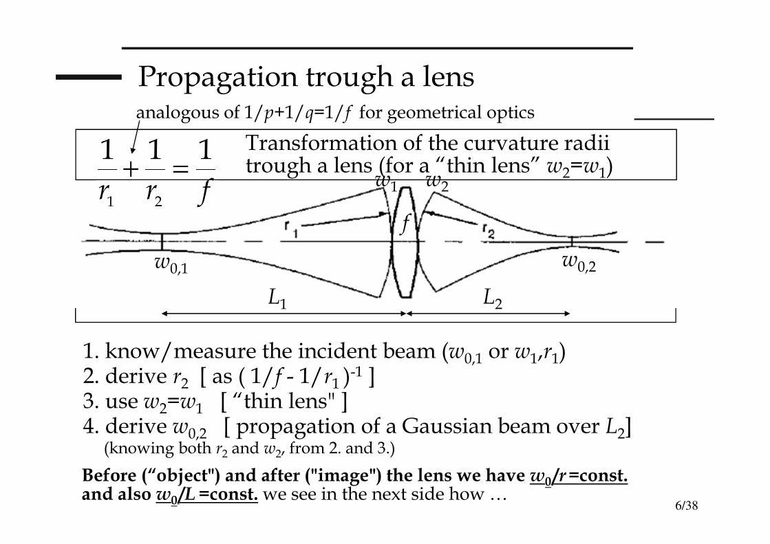
Propagation trough a lens
f
Transformation of the curvature radii trough a lens (for a “thin lens” w2=w1)
w0,1 w0,2
L1 L2
1. know/measure the incident beam (w0,1 or w1,r1) 2. derive r2 [ as ( 1/f - 1/r1 )
-1 ]3. use w2=w1 [ “thin lens" ] 4. derive w0,2 [ propagation of a Gaussian beam over L2]
(knowing both r2 and w2, from 2. and 3.)
Before (“object") and after ("image") the lens we have w0 /r=const.and also w0 /L=const.we see in the next side how …
analogous of 1/p+1/q=1/f for geometrical optics
w1 w2

7/38
Propagation through a lens
To “enlarge" w0,1 with respect to w0,2, one must work with r1>r2 and hence with the lens more distant from w0,1 (L1>L2) then the distance from w0,2 (or for L1<L2 one has w0,1<w0,2)
f
Transformation of the radii of curvature through a lens (for a thin lens w2=w1)
w0,1 w0,2
L1 L2
After propagating through a lens the beam undergoes a magnification m=w0,2 /w0,1=r2 /r1=L2 /L1
If z>zR (z>>zR) ⇒⇒⇒⇒ r1,2≅≅≅≅L1,2 and hence θ1r1≅w1=w2≅θ2r2 ⇒r1/w0,1 ≅r2 /w0,2 w0,1 /w0,2≅≅≅≅r1 /r2≅≅≅≅L1 /L2 e w0,1 /L1≅≅≅≅w0,2 /L2
being θθθθ=λλλλ/ππππw0
w1 w2
r1,2 are not easy to measure while measuring L1,2 is simple
8/38
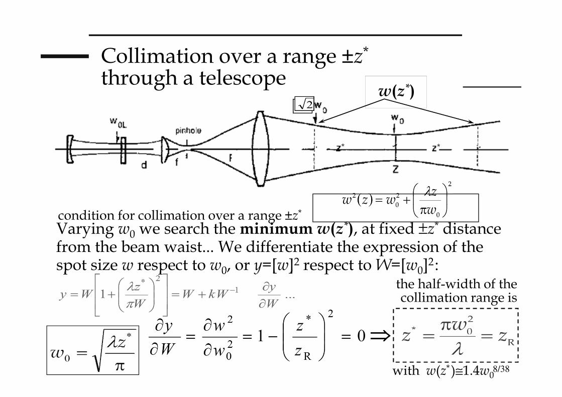
Collimation over a range ±z*
through a telescope
**
w(z*)
Varying w0 we search the minimum w(z*), at fixed ±z* distancefrom the beam waist... We differentiate the expression of the spot size w respect to w0, or y=[w]
2 respect to W=[w0]2:
condition for collimation over a range ±z*
⇒⇒⇒⇒
the half-width of the collimation range is
with w(z*)≅1.4w0
k

9/38
Beam-sizing of the laser spotafter a telescope
**
w0,f
w0,f /w0L≅≅≅≅f /d e w0 /w0,f ≅≅≅≅Z /F ⇒⇒⇒⇒ w0 ≅≅≅≅ (Z /F) ⋅⋅⋅⋅(f /d)w0L
Spot magnification: m=w0 /w0L=(Z/d)⋅(1/M)with M = F / f = wF / wf telescope magnification
Typically one has f<<F, and it is relatively easy to “adjust" the dimension w0 (∝f ) and the distance Z by slightly moving the ocular (lens with focal length f )( in fact, in terms of relative variations: ∆w0/w0 = ∆f/f )
wf
wF

10/38
Example of collimation of an He-Ne LASER for alignment
DATA:He-Ne LASER with plano-concave cavity (L=20 cm, ROC=1 m).We want to cover ±±±±z*=±±±±20 m with minimum spot dimensions:calculate the magnification m of the laser spot and the one M of the telescope.
From we obtain w0L=282 µµµµm ≈≈≈≈ 0.3 mm
From =20 m we obtain w0=2 mm (diam. 2w0=4 mm)
Imagine we use a telescope with ocular distance d=10 cmand we want to work with Z≅z*=20 m.
From w0 ≅ (Z/F) ⋅ ( f/d)w0L we get m=w0/w0L= 7.1 = (Z/d)/M as magnification of the laser spot, whereas the magnification of the telescope is M = F/f = (Z/d)/m = (20/0.1)/7.1 = 28
At ±20 m from w0, beam size is D≅≅≅≅2 ⋅1.41w0 ≅ 2.8 ⋅2mm= 5.6mm
CS7

Diapositiva 10
CS7 qui termina la 6a lezione dell'AA 2005/2006Cesare Svelto; 31/03/2006
11/38
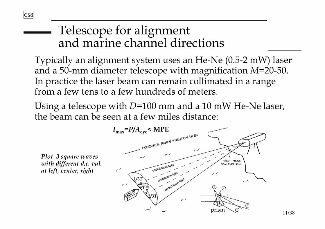
Telescope for alignment and marine channel directions
Typically an alignment system uses an He-Ne (0.5-2 mW) laser and a 50-mm diameter telescope with magnification M=20-50. In practice the laser beam can remain collimated in a range from a few tens to a few hundreds of meters.
Using a telescope with D=100 mm and a 10 mW He-Ne laser, the beam can be seen at a few miles distance:
2/3T
1/3T
T
prism
Imax=P/Aeye< MPE
Plot 3 square waveswith different d.c. val. at left, center, right
CS8

Diapositiva 11
CS8 qui inizia la 7a lezione dell'AA 2005/2006Cesare Svelto; 05/04/2006
12/38
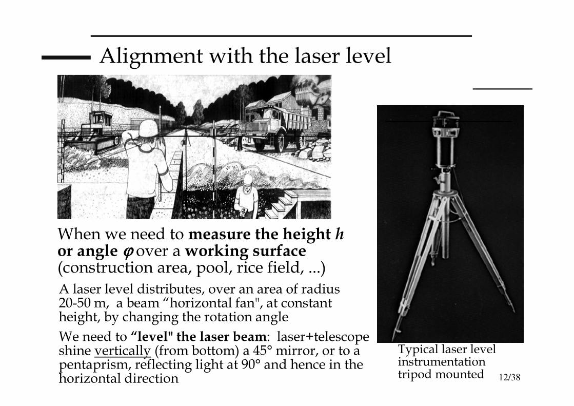
Alignment with the laser level
When we need to measure the height hor angle ϕϕϕϕ over a working surface(construction area, pool, rice field, ...)
A laser level distributes, over an area of radius 20-50 m, a beam “horizontal fan", at constant height, by changing the rotation angle
Typical laser level instrumentation tripod mounted
We need to “level" the laser beam: laser+telescope shine vertically (from bottom) a 45° mirror, or to a pentaprism, reflecting light at 90° and hence in the horizontal direction
13/38
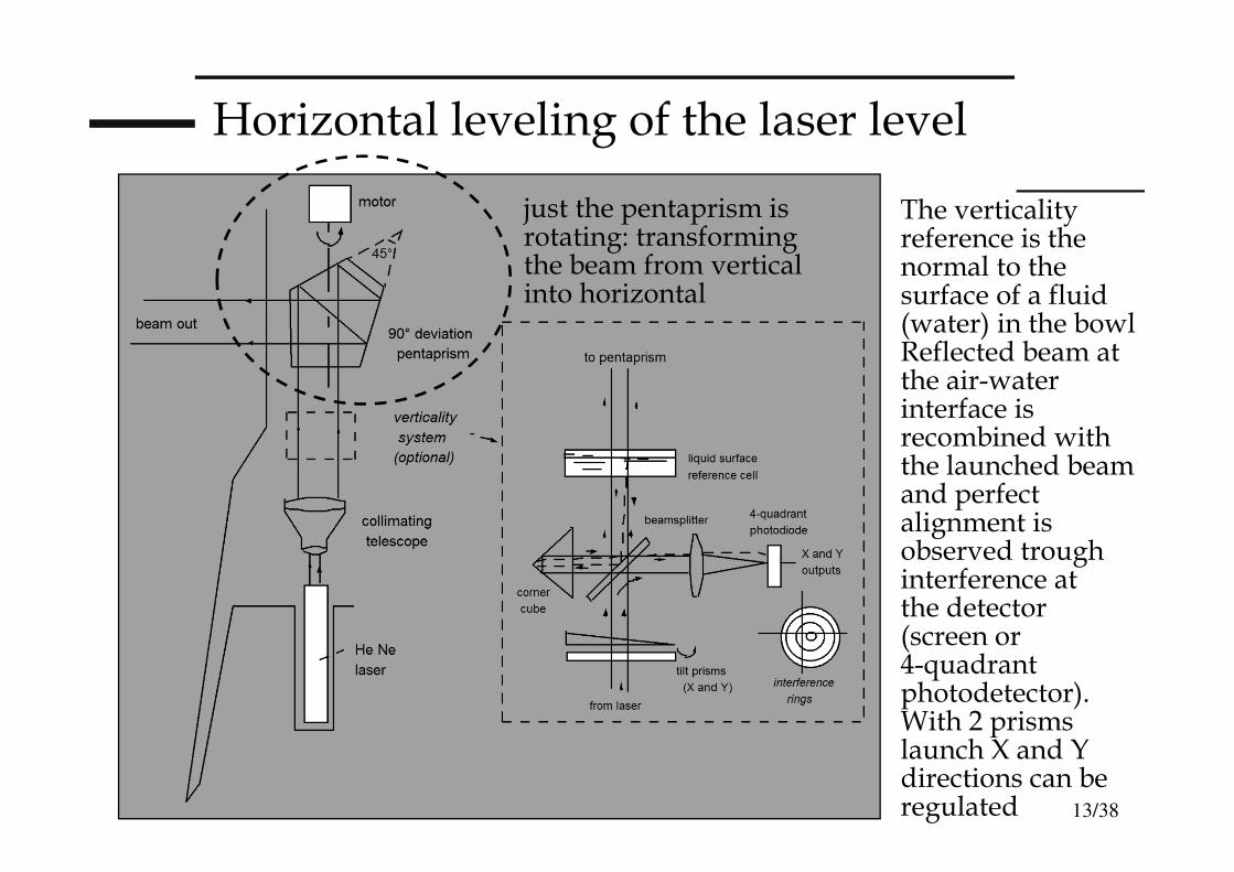
Horizontal leveling of the laser level
The verticality reference is the normal to the surface of a fluid (water) in the bowl Reflected beam at the air-water interface is recombined with the launched beam and perfect alignment is observed trough interference at the detector(screen or 4-quadrant photodetector).With 2 prisms launch X and Y directions can be regulated
just the pentaprism is rotating: transforming the beam from vertical into horizontal

14/38
Beam centering on the target and position-sensitive photodetectors
For less stringent applications, like in constructions, it is sufficient an eye alignment (∆x≈∆y≈1mm)
For more accurate measurements, we use a photodetector to provide for an electric signal proportional to the alignment error. A feedback system allows the alignment control by minimizing the error signal.
The position-sensitive photodetector can be a special “photodiode” (4-quadrant photodiode, PSD sensor or even a CCD) or a normal photodiode coupled to a spatial reticule/mask (rotating reticule) transmitting light as a function of the impinging beam position
15/38
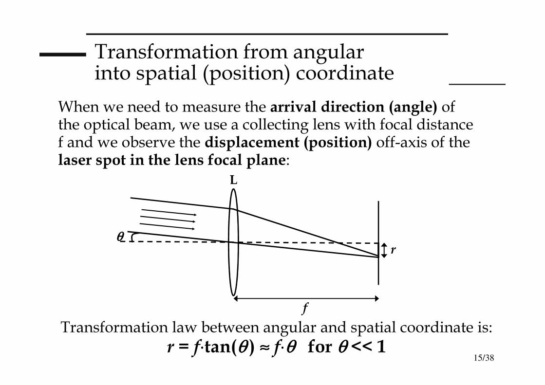
Transformation from angular into spatial (position) coordinate
When we need to measure the arrival direction (angle) of the optical beam, we use a collecting lens with focal distance f and we observe the displacement (position) off-axis of the laser spot in the lens focal plane:
Transformation law between angular and spatial coordinate is:
r = f⋅⋅⋅⋅tan(θθθθ ) ≈≈≈≈ f⋅⋅⋅⋅θθθθ for θθθθ << 1
θθθθ
f
r
L
16/38
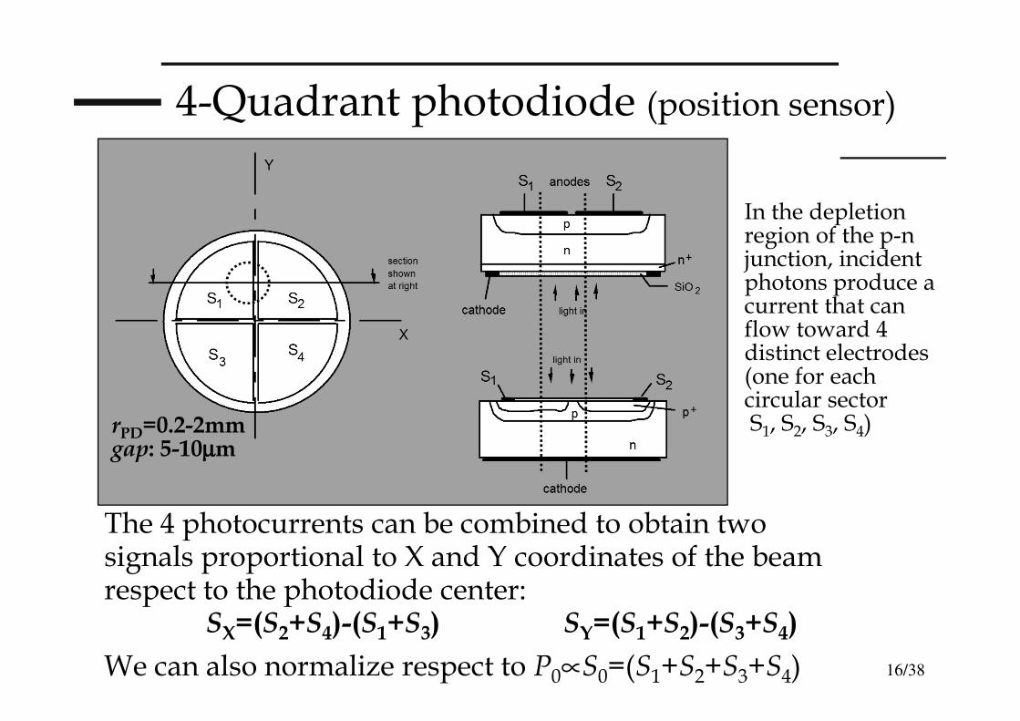
4-Quadrant photodiode (position sensor)
In the depletion region of the p-n junction, incident photons produce a current that can flow toward 4 distinct electrodes (one for each circular sectorS1, S2, S3, S4)
The 4 photocurrents can be combined to obtain two signals proportional to X and Y coordinates of the beam respect to the photodiode center:
SX=(S2+S4)-(S1+S3) SY=(S1+S2)-(S3+S4)
rPD=0.2-2mmgap: 5-10µµµµm
We can also normalize respect to P0∝S0=(S1+S2+S3+S4)
17/38
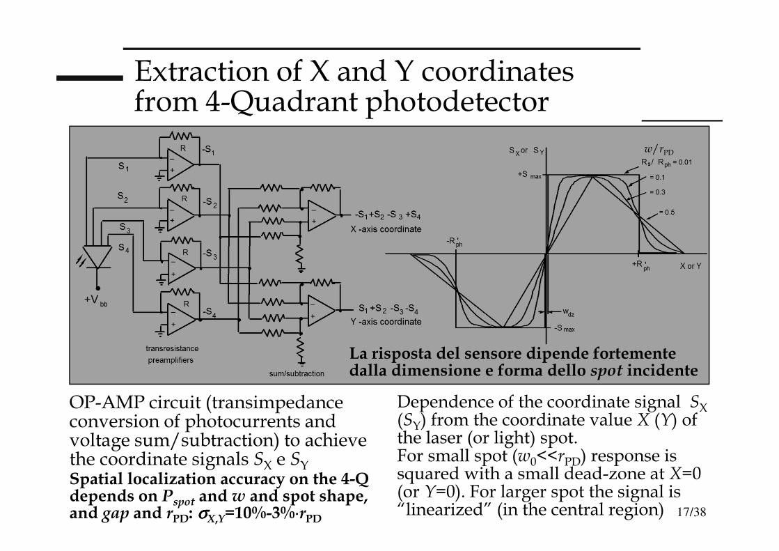
Extraction of X and Y coordinates from 4-Quadrant photodetector
Dependence of the coordinate signal SX(SY) from the coordinate value X (Y) of the laser (or light) spot.For small spot (w0<<rPD) response is squared with a small dead-zone at X=0 (or Y=0). For larger spot the signal is “linearized” (in the central region)
OP-AMP circuit (transimpedance conversion of photocurrents and voltage sum/subtraction) to achieve the coordinate signals SX e SY
La risposta del sensore dipende fortemente dalla dimensione e forma dello spot incidente
w/rPD
Spatial localization accuracy on the 4-Q depends on Pspot and w and spot shape, and gap and rPD: σσσσX,Y=10%-3%⋅⋅⋅⋅rPD
18/38
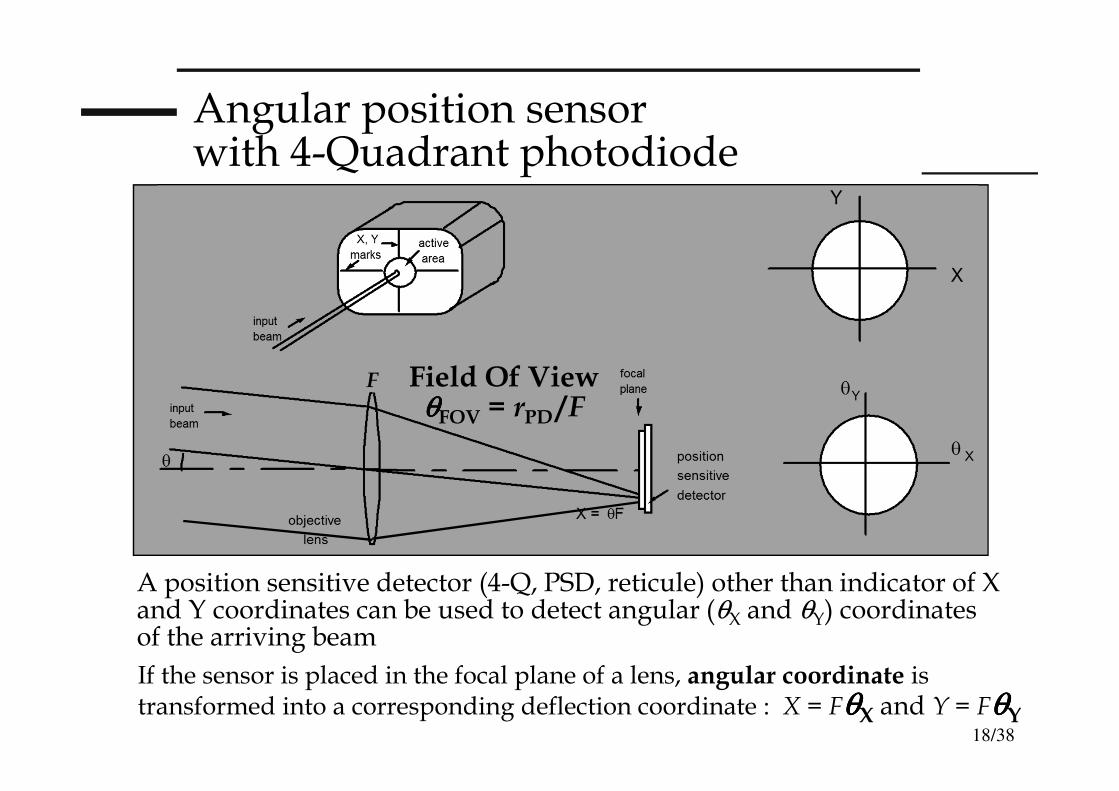
Angular position sensor with 4-Quadrant photodiode
If the sensor is placed in the focal plane of a lens, angular coordinate is transformed into a corresponding deflection coordinate : X = FθθθθX and Y = FθθθθY
A position sensitive detector (4-Q, PSD, reticule) other than indicator of X and Y coordinates can be used to detect angular (θX and θY) coordinates of the arriving beam
Field Of View θθθθFOV = rPD /F
F

19/38
PSD photodiode (scheme and principle)
Position Sensitive Detectoris a normal PIN photodiode with thin p and n regions lightly doped (to enhance the series resistance of p and n volumes at the border of the depletion region)Incident spot of (X,Y) coordinate produces a photocurrent flowing from electrodes Y (cathode) to electrodes X (anode)
The current, passing trough regions p and n of high resistivity is divided with the partitions rule between two resistors.The difference in the detected currents on the same electrode pairs (X or Y) gives the coordinate (X o Y)
'Si' for λλλλ=400-1100 nmwith L=0.5-5 mm
left right
the photodiode is reverse bias polarized
High linearity over the whole measurement range
20/38
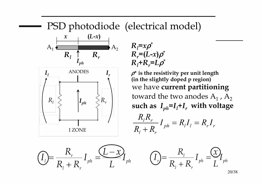
PSD photodiode (electrical model)
Rl=xρρρρ*
Rr=(L-x)ρρρρ*
Rl+Rr=Lρρρρ*
ρρρρ* is the resistivity per unit length (in the slightly doped p region)
we have current partitioningtoward the two anodes A1 , A2
such as Iph=Il+Ir
Il
RrRl
ANODES
I ZONE
Iph
Ir
Rl RrIph
x (L-x)
A1 A2
with voltage

21/38
PSD photodiode (working equations)
Similarly
From the OP-AMP circuit we obtain
The output becomes independent from photocurrent Iph (and P) dividing for the sum signal ΣX/Y=R(Ix/y1+Ix/y2)=RIph⇒measurement independent from P and ≈responsivity ( ρ )
Iph=ρPvarying with P(and also with ρ!)

22/38
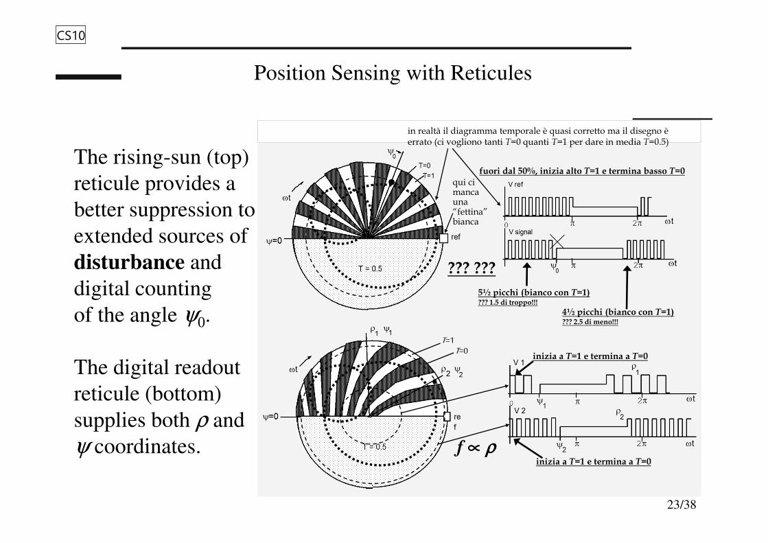
Position Sensing with Reticules
Position sensing by a rotating
reticule: light from a bright spot at
the angle θ is imaged by the
objective lens on the focal plane,
where it is chopped by the reticule
placed in front of the photodetector.
By comparing the phase-shift of
the square waveform from the
photodetector and of a reference,
the angular position ψψψψ0 of the
source is determined.
The amplitude of the signal, Vsignal ,
carries information on the polar
coordinate ρρρρ, similar to that of the
quadrant PD.
ρRP
D
Transformation from angular into spatial coordinate (lens focal plane) and measurement of spatial coordinate (x,y) from polar coordinates (ρ ,θ =Ψ0)
23/38
Position Sensing with Reticules
The rising-sun (top)
reticule provides a
better suppression to
extended sources of
disturbance and
digital counting
of the angle ψ0.
The digital readout
reticule (bottom)
supplies both ρ and
ψ coordinates.
??? ???
fuori dal 50%, inizia alto T=1 e termina basso T=0
inizia a T=1 e termina a T=0
inizia a T=1 e termina a T=0
f ∝∝∝∝ ρρρρ
T=1
T=0
5½ picchi (bianco con T=1)??? 1.5 di troppo!!!
4½ picchi (bianco con T=1)??? 2.5 di meno!!!
in realtà il diagramma temporale è quasi corretto ma il disegno è errato (ci vogliono tanti T=0 quanti T=1 per dare in media T=0.5)
qui ci mancauna “fettina”bianca
CS10
Diapositiva 23
CS10 qui termina la 7a lezione dell'AA 2005/2006Cesare Svelto; 05/04/2006

24/38
angular distribution is I(θθθθ ) = E02 ////ηηηη0000 ⋅⋅⋅⋅ sinc2 ππππθθθθ /θθθθD
first zeroes of sinc are at θD=θdiff.=±λ/D e Xzero=±Fλ/D
hence we can obtain D = Fλλλλ////Xzero
D
Measurements wires diametersfrom diffracted light analysis
electric field on the detector is the Fourier transform of the aperture:transf. of rectangle is sinc[ππππθθθθ/(λλλλ/D)]
θθθθD
∝∝∝∝
For small wires (small D) we have Xzero large and vice versa(it is easier – higher sensitivity – to measure wires with small diameter)
=θ /θdiff.
The distance between zeroes (or peaks) on the detector is proportional to 1/D
CS11

Diapositiva 24
CS11 qui inizia la 8a lezione dell'AA 2005/2006Cesare Svelto; 05/04/2006
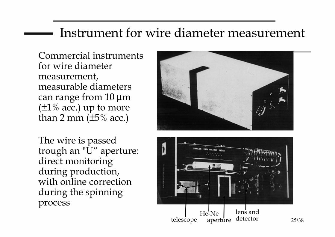
25/38
Commercial instruments for wire diameter measurement, measurable diameters can range from 10 µm (±1% acc.) up to more than 2 mm (±5% acc.)
aperture telescopeHe-Ne lens and
detector
Instrument for wire diameter measurement
The wire is passed trough an "U“ aperture: direct monitoring during production, with online correction during the spinning process

26/38
The diameter analyzer measures diffracted light from suspendedparticles within a fluid. At the cell exit a lens converts angulardiffraction profile into a corresponding spatial profile in the focalplane (θ R). A photodetector (scanned PD or CCD) measures I(R):the distribution of particle diameters, p(D), is calculated inverting
LAELS: Low-Angle ELastic Scatteringelectric field on the detector is the Fourier transform of the aperture:transf. of circle is somb[(R/F)/(λλλλ/D)]
I(R) = I0 ∫∫∫∫0-∞ somb2[(D/λλλλ)(R/F)]⋅⋅⋅⋅ p(D) dD with(R/F)=tanθθθθ ≅≅≅≅θθθθ
somb(x)=2[J1(ππππx)]/ππππx
Particle diameter measurement
[(θθθθ /θθθθdiff.)]
27/38
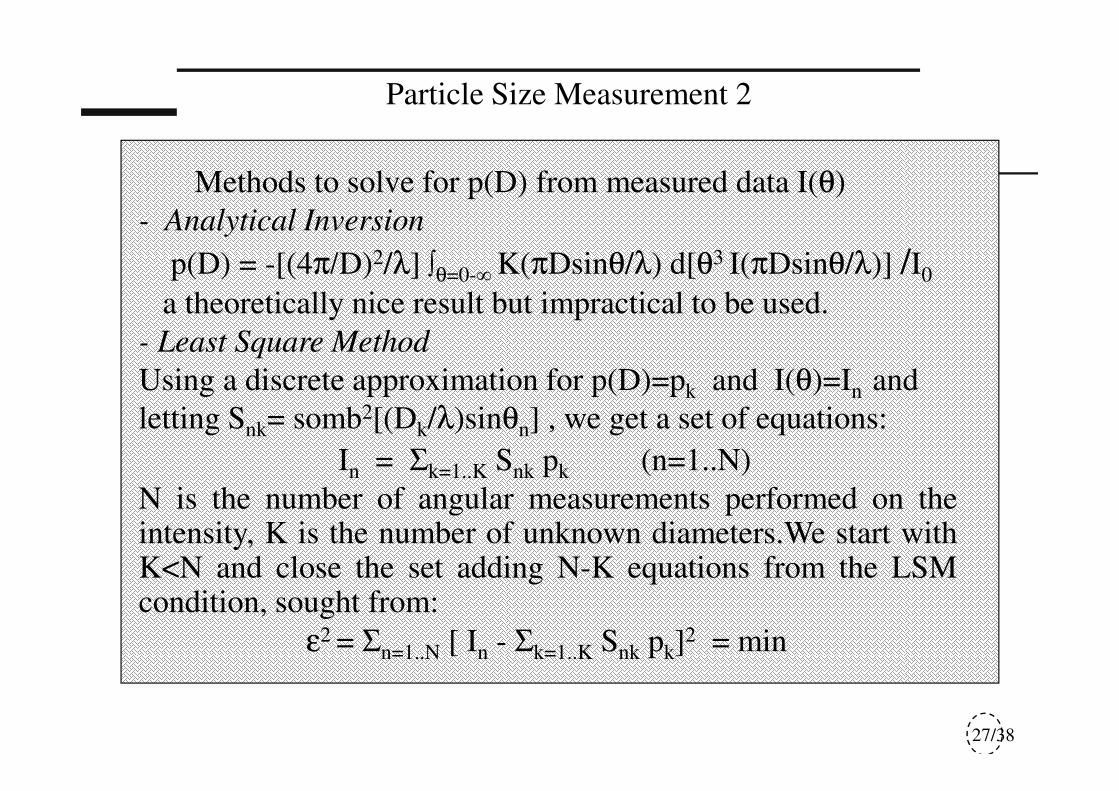
Particle Size Measurement 2
Methods to solve for p(D) from measured data I(θ)
- Analytical Inversion
p(D) = -[(4π/D)2/λ] ∫θ=0-∞ K(πDsinθ/λ) d[θ3 I(πDsinθ/λ)] /I0
a theoretically nice result but impractical to be used.
- Least Square Method
Using a discrete approximation for p(D)=pk and I(θ)=In and
letting Snk= somb2[(Dk/λ)sinθn] , we get a set of equations:
In = Σk=1..K Snk pk (n=1..N)
N is the number of angular measurements performed on theintensity, K is the number of unknown diameters.We start withK<N and close the set adding N-K equations from the LSMcondition, sought from:
ε2 = Σn=1..N [ In - Σk=1..K Snk pk]2 = min

28/38
Particle Size Measurement 3
Taking the derivative respect pk‘s and equating to zero gives:
0 = ∂(ε2)/∂pk = Σn=1..N 2[ In - Σk=1..K Snk pk](-Snk)
and rearranging we get
Jh = Σk=1..K Zhk pk (h=1..K)
where we have let Jh =Σn=1..N InSnh and Znk= Σn=1..N Snk2
Now, the number of equations is equal to the number of unknown and we can
solve for pk with standard algebra.Usually, the range of diameters
of interest may be large (for
example, two decades from 2 to
200µm) but the number of
affordable diameter is modest
(e.g. K=6-9) at ±10% accuracy.
29/38
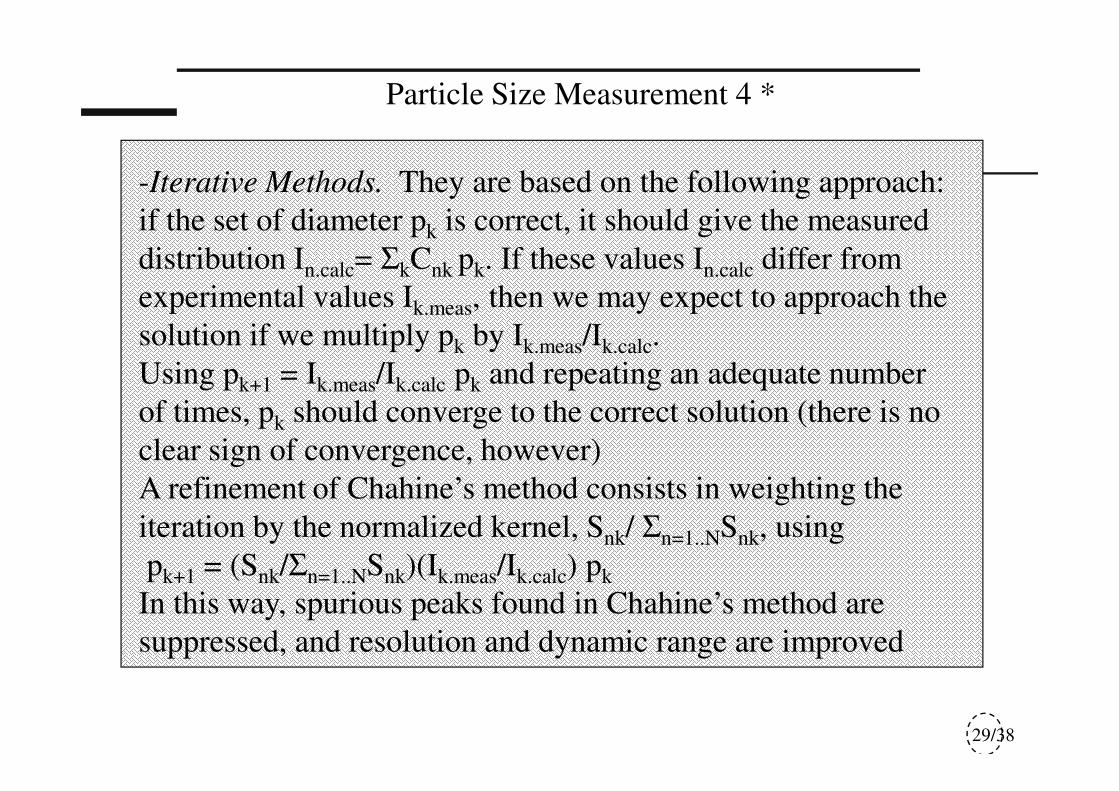
Particle Size Measurement 4 *
-Iterative Methods. They are based on the following approach:
if the set of diameter pk is correct, it should give the measured
distribution In.calc= ΣkCnk pk. If these values In.calc differ from
experimental values Ik.meas, then we may expect to approach the
solution if we multiply pk by Ik.meas/Ik.calc.
Using pk+1 = Ik.meas/Ik.calc pk and repeating an adequate number
of times, pk should converge to the correct solution (there is no
clear sign of convergence, however)
A refinement of Chahine’s method consists in weighting the
iteration by the normalized kernel, Snk/ Σn=1..NSnk, using
pk+1 = (Snk/Σn=1..NSnk)(Ik.meas/Ik.calc) pk
In this way, spurious peaks found in Chahine’s method are
suppressed, and resolution and dynamic range are improved

30/38
Particle Size Measurement 5 *
Common errors in the PSM: finite size of detector, beam waist effects, lens
vignetting, and undiffracted beam (θ=0), important for small θ (large D).
Better than a stop to block it out, we can use the filtering known as reverse
Fourier-transform illumination, with a convergent beam to illuminate the
cell. Diffracted rays (dotted lines) are focused on axis, and pass through the
pinhole, whereas undiffracted rays arrive out-of-axis and are blocked.
31/38
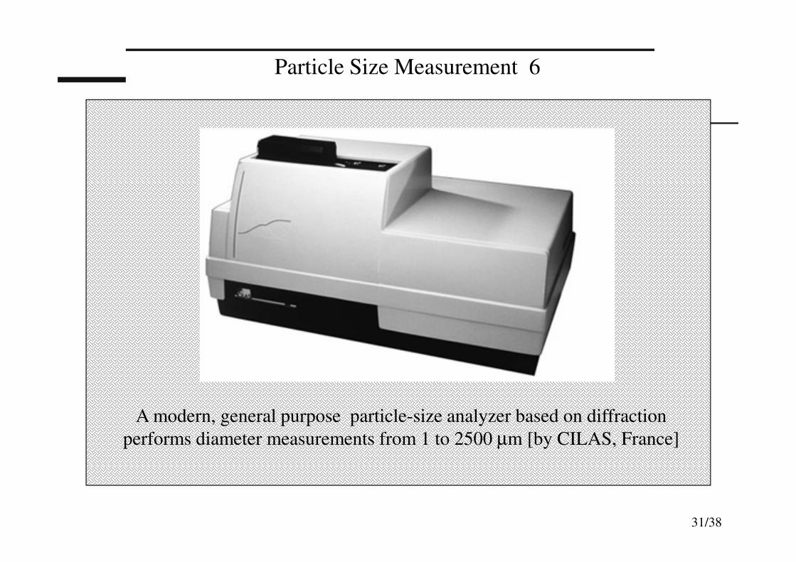
Particle Size Measurement 6
A modern, general purpose particle-size analyzer based on diffraction
performs diameter measurements from 1 to 2500 µm [by CILAS, France]
32/38
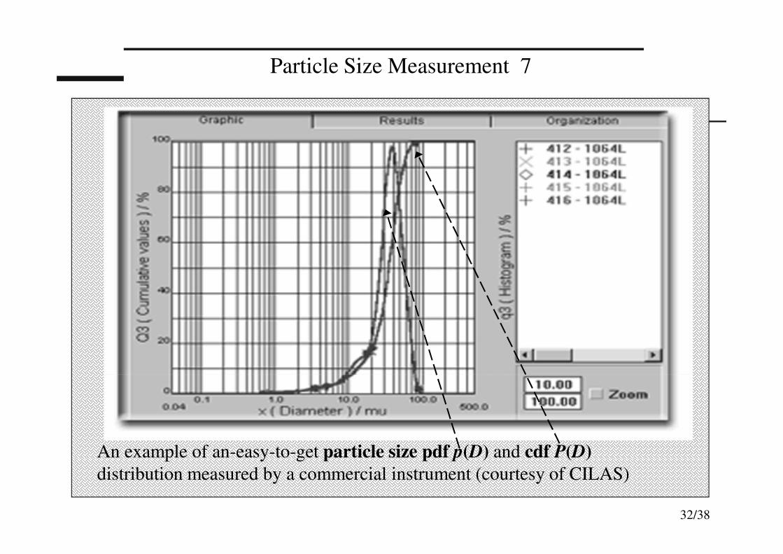
Particle Size Measurement 7
An example of an-easy-to-get particle size pdf p(D) and cdf P(D)
distribution measured by a commercial instrument (courtesy of CILAS)
33/38
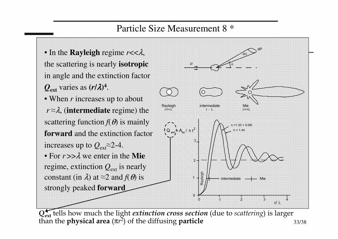
Particle Size Measurement 8 *
• In the Rayleigh regime r<<λ,
the scattering is nearly isotropic
in angle and the extinction factor
Qext varies as (r/λλλλ)4.
• When r increases up to about
r ≈λ, (intermediate regime) the
scattering function f(θ) is mainly
forward and the extinction factor
increases up to Qext≈2-4.
• For r >>λ we enter in the Mie
regime, extinction Qext is nearly
constant (in λ) at ≈2 and f(θ) is
strongly peaked forward
Qext tells how much the light extinction cross section (due to scattering) is larger than the physical area (πr2) of the diffusing particle
34/38
Particle Size Measurement 9 *
• Another method is SEAS (Spectral Extinction Aerosol Sizing). It is based
on measuring light scattered from the cell at a fixed angle, while scanning λinstead of θ. By varying the ratio D/λ, the extinction factor Qext(D,λ,n) varies
and the scattered power too, according to:
I(λ,45°) = f(45°) (∆Ω/4π) I0 ∫0-∞ Qext(D,λ,n) p(D) dD
where f(θ)=scattering function, Qext=extinction factor. The equation is the
counterpart of that for extinction-related measurement, and all the methods of
inversion of the Fredholm’s integral can now be applied on Dk and λn. With
SEAS we may to go down to 0.02–0.1µµµµm as the minimum measurable size,
overlapping with the LAELS low-range (≈ 2-5 µm).
• A last method is the Dynamical Scattering Size Analyzer (DSSA), useful
for very small (1..100-nm) particles. Based on the frequency shift due to
Doppler effect (ko-ki). v, it is measured by the time-domain autocorrelation
function C(τ)=(1/T)∫0-Ti(t)i(t+τ)dt which depends from the diffusion constant
δ of particles according to: C(τ)=C0 exp –δ (ko-ki)2τ.

35/38
Particle Size Measurement 10
A SEAS particle size analyzer uses scattering data at 135° to sort
submicronic particulate (typ. of metropolitan area pollutants) from 0.02 to
0.1 µm [by CILAS, France]

36/38
Particle Size Measurement 11
A modern particle-size analyzer based on diffraction and extinction
(LAELS + SEAS), performs diameter measurements
from 0.05 to 2500 µm [by CILAS, France]
37/38
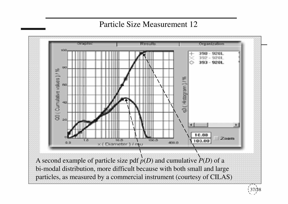
Particle Size Measurement 12
A second example of particle size pdf p(D) and cumulative P(D) of a
bi-modal distribution, more difficult because with both small and large
particles, as measured by a commercial instrument (courtesy of CILAS)

38/38
Particle Size Measurement 13
A third example of particle size pdf p(D) and cumulative P(D) of a
distribution with two populations of very large particles (powders) as
measured by a commercial granulometer (courtesy of CILAS)