Optical beam classification using deep learning: A comparison with

rule- and feature-based classification

Md. Zahangir Alomab, Abdul A. S. Awwalb, Roger Lowe-Webb, Tarek M. Tahaa

aDepartment of Electrical and Computer Engineering, University of Dayton, Dayton, Ohio 45469;

bNational Ignition Facility (NIF), Lawrence Livermore National Laboratory, Livermore,

California 94551.

ABSTRACT

Deep-learning methods are gaining popularity because of their state-of-the-art performance in image classification tasks.

In this paper, we explore classification of laser-beam images from the National Ignition Facility (NIF) using a novel deep-

learning approach. NIF is the world’s largest, most energetic laser. It has nearly 40,000 optics that precisely guide, reflect,

amplify, and focus 192 laser beams onto a fusion target. NIF utilizes four petawatt lasers called the Advanced Radiographic

Capability (ARC) to produce backlighting X-ray illumination to capture implosion dynamics of NIF experiments with

picosecond temporal resolution. In the current operational configuration, four independent short-pulse ARC beams are

created and combined in a split-beam configuration in each of two NIF apertures at the entry of the pre-amplifier. The sub-

aperture beams then propagate through the NIF beampath up to the ARC compressor. Each ARC beamlet is separately

compressed with a dedicated set of four gratings and recombined as sub-apertures for transport to the parabola vessel,

where the beams are focused using parabolic mirrors and pointed to the target. Small angular errors in the compressor

gratings can cause the sub-aperture beams to diverge from one another and prevent accurate alignment through the

transport section between the compressor and parabolic mirrors. This is an off-normal condition that must be detected and

corrected. The goal of the off-normal check is to determine whether the ARC beamlets are sufficiently overlapped into a

merged single spot or diverged into two distinct spots. Thus, the objective of the current work is three-fold: developing a

simple algorithm to perform off-normal classification, exploring the use of Convolutional Neural Network (CNN) for the

same task, and understanding the inter-relationship of the two approaches. The CNN recognition results are compared with

other machine-learning approaches, such as Deep Neural Network (DNN) and Support Vector Machine (SVM). The

experimental results show around 96% classification accuracy using CNN; the CNN approach also provides comparable

recognition results compared to the present feature-based off-normal detection. The feature-based solution was developed

to capture the expertise of a human expert in classifying the images. The misclassified results are further studied to explain

the differences and discover any discrepancies or inconsistencies in current classification.

Keywords: Deep Learning, CNN, DBN, SVM, feature extraction, beam classification.

1. INTRODUCTION

The National Ignition Facility (NIF) is the world’s largest, most energetic laser. It has nearly 40,000 optics that precisely

guide, reflect, amplify, and focus 192 laser beams onto a fusion target, and thus provides a platform for performing high-

energy laser physics experiments [1,2]. A diagnostic known as the Advanced Radiographic Capability (ARC) was

developed to properly understand the implosion dynamics [3,4]. ARC produces backlighting high-energy X-ray beams

that can penetrate and image the implosion as it is happening. Currently, four independent short-pulse ARC beams are

created and combined in a split-beam configuration in each of two NIF apertures at the entry of the pre-amplifier. The

sub-aperture beams are amplified using NIF hardware as they propagate through the NIF beampath up to the ARC

compressor. Each ARC beamlet is separately compressed with a set of four gratings and recombined as sub-apertures for

transport to the parabola vessel, where the beams are focused using parabolic mirrors and pointed to the target. Small

angular deviations in the compressor gratings can introduce pointing errors in the sub-aperture beams and cause them to

diverge from one another. This prevents accurate alignment through the transport section between the compressor and

parabolic mirrors. This off-normal condition must be identified using Automatic Alignment (AA) algorithms [5] and

corrected before continuing with the ARC shot [6]. The off-normal check determines whether the ARC beamlets are

merged into a single spot or have diverged into two distinct spots. Typical examples of single- and double-spot ARC

alignment beam images and the ARC beamlets are shown in Figure 1.

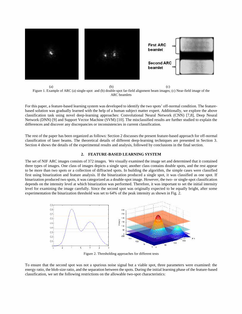
(a) (b) (c)

Figure 1. Example of ARC (a) single-spot and (b) double-spot far-field alignment beam images; (c) Near-field image of the

ARC beamlets

For this paper, a feature-based learning system was developed to identify the two spots’ off-normal condition. The feature-

based solution was gradually learned with the help of a human subject matter expert. Additionally, we explore the above

classification task using novel deep-learning approaches: Convolutional Neural Network (CNN) [7,8], Deep Neural

Network (DNN) [9] and Support Vector Machine (SVM) [10]. The misclassified results are further studied to explain the

differences and discover any discrepancies or inconsistencies in current classification.

The rest of the paper has been organized as follows: Section 2 discusses the present feature-based approach for off-normal

classification of laser beams. The theoretical details of different deep-learning techniques are presented in Section 3.

Section 4 shows the details of the experimental results and analysis, followed by conclusions in the final section.

2. FEATURE-BASED LEARNING SYSTEM

The set of NIF ARC images consists of 372 images. We visually examined the image set and determined that it contained

three types of images. One class of images depicts a single spot; another class contains double spots, and the rest appear

to be more than two spots or a collection of diffracted spots. In building the algorithm, the simple cases were classified

first using binarization and feature analysis. If the binarization produced a single spot, it was classified as one spot. If

binarization produced two spots, it was categorized as a double-spot image. However, the two- or single-spot classification

depends on the intensity level at which binarization was performed. Therefore, it was important to set the initial intensity

level for examining the image carefully. Since the second spot was originally expected to be equally bright, after some

experimentation the binarization threshold was set to 64% of the peak intensity as shown in Fig. 2.

Figure 2. Thresholding approaches for different tests

To ensure that the second spot was not a spurious noise signal but a viable spot, three parameters were examined: the

energy ratio, the blob-size ratio, and the separation between the spots. During the initial learning phase of the feature-based

classification, we set the following restrictions on the allowable two-spot characteristics:

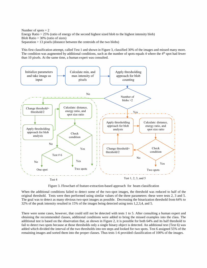
Number of spots = 2

Energy Ratio > 25% (ratio of energy of the second highest sized blob to the highest intensity blob)

Blob Ratio > 30% (ratio of sizes)

Separation > 13 pixels (distance between the centroids of the two blobs)

This first classification attempt, called Test 1 and shown in Figure 3, classified 30% of the images and missed many more.

The condition was augmented by additional conditions, such as the number of spots equals 4 where the 4th spot had fewer

than 10 pixels. At the same time, a human expert was consulted.

Figure 3. Flowchart of feature-extraction-based approach for beam classification

When the additional conditions failed to detect some of the two-spot images, the threshold was reduced to half of the

original threshold. Tests were then performed using similar values of the three parameters: these were tests 2, 3 and 5.

The goal was to detect as many obvious two-spot images as possible. Decreasing the binarization threshold from 64% to

32% of the peak intensity resulted in 15% of the images being detected using tests 1,2,3,4, and 5.

There were some cases, however, that could still not be detected with tests 1 to 5. After consulting a human expert and

obtaining the recommended classes, additional conditions were added to bring the missed examples into the class. The

additional test is based on the observation that, as shown in Figure 2, it is possible for both 64% and its half threshold to

fail to detect two spots because at those thresholds only a single binary object is detected. An additional test (Test 6) was

added which divided the interval of the two thresholds into ten steps and looked for two spots. Test 6 assigned 55% of the

remaining images and sorted them into the proper classes. Thus tests 1-6 provided classification of 100% of the images.

Initialize parameters

and take image as

input

Calculate min, and

max intensity of

pixels

Apply thresholding

approach for blob

counting

Change threshold=

threshold/2

Apply thresholding

approach for blob

analysis

Calculate: distance,

energy ratio, and

spot size ratio

Check

condition

Test # 6

One spot Two spots

Test 4 Test 1, 2, 3, and 5

Number of

blobs >2

Apply thresholding

approach for blob

analysis

Calculate: distance,

energy ratio, and

spot size ratio

Change threshold=

threshold/2 Check

condition

Two spots

No

Yes

Yes

Yes

Yes No

No

No

3. DEEP-LEARNING METHODS

3.1 Convolutional Neural Network (CNN)

The CNN architecture was proposed by Fukushima in 1980 [11]. It was not widely used, however, because the training

algorithm required high computational power. In 1998, Lacuna et al. applied a gradient-based learning algorithm to CNN

and obtained successful results in different application domains including image processing, computer vision, machine

learning, and others [7,8,12].

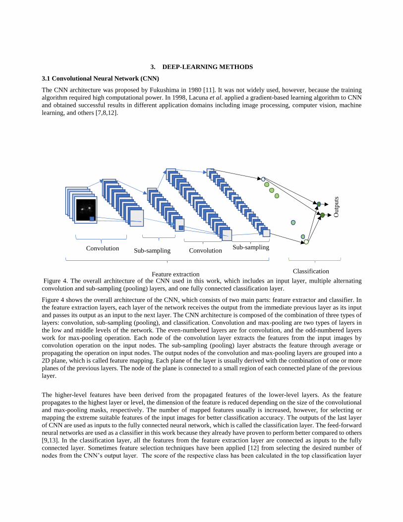
Figure 4. The overall architecture of the CNN used in this work, which includes an input layer, multiple alternating

convolution and sub-sampling (pooling) layers, and one fully connected classification layer.

Figure 4 shows the overall architecture of the CNN, which consists of two main parts: feature extractor and classifier. In

the feature extraction layers, each layer of the network receives the output from the immediate previous layer as its input

and passes its output as an input to the next layer. The CNN architecture is composed of the combination of three types of

layers: convolution, sub-sampling (pooling), and classification. Convolution and max-pooling are two types of layers in

the low and middle levels of the network. The even-numbered layers are for convolution, and the odd-numbered layers

work for max-pooling operation. Each node of the convolution layer extracts the features from the input images by

convolution operation on the input nodes. The sub-sampling (pooling) layer abstracts the feature through average or

propagating the operation on input nodes. The output nodes of the convolution and max-pooling layers are grouped into a

2D plane, which is called feature mapping. Each plane of the layer is usually derived with the combination of one or more

planes of the previous layers. The node of the plane is connected to a small region of each connected plane of the previous

layer.

The higher-level features have been derived from the propagated features of the lower-level layers. As the feature

propagates to the highest layer or level, the dimension of the feature is reduced depending on the size of the convolutional

and max-pooling masks, respectively. The number of mapped features usually is increased, however, for selecting or

mapping the extreme suitable features of the input images for better classification accuracy. The outputs of the last layer

of CNN are used as inputs to the fully connected neural network, which is called the classification layer. The feed-forward

neural networks are used as a classifier in this work because they already have proven to perform better compared to others

[9,13]. In the classification layer, all the features from the feature extraction layer are connected as inputs to the fully

connected layer. Sometimes feature selection techniques have been applied [12] from selecting the desired number of

nodes from the CNN’s output layer. The score of the respective class has been calculated in the top classification layer

Feature extraction Classification

Convolution Sub-sampling Convolution

Outp

uts

Sub-sampling

using the softmax layer. Based on the highest score, the classifier gives outputs for the corresponding classes after finishing

the propagation. Mathematical details on different layers of CNN are discussed in the following section.

3.1.1 Convolutional layer

In this layer, the feature maps of the previous layer are convolved with a learnable kernel such as random or Gabor. In this

implementation, random filters are used. The outputs of the kernel go through linear or non-linear activation functions of

Rectified Linear Unit (ReLU) to form the output feature maps. Each of the output feature maps can be combined with

more than one input feature map. In general, we have that

𝑥𝑗𝑙 = 𝑓 (∑ 𝑥𝑖

𝑙−1𝑖𝜖𝑀𝑗

∗ 𝑘𝑖𝑗𝑙 + 𝑏𝑗

𝑙) (1)

where 𝑥𝑗𝑙 is the output of the current layer, 𝑥𝑖

𝑙−1 is previous layer output, 𝑘𝑖𝑗𝑙 is the kernel for the present layer, and 𝑏𝑗

𝑙 is

the bias for the current layer. 𝑀𝑗 represents a selection of input maps. For each output map is given an additive bias 𝑏. The

input maps, however, will be convolved with distinct kernels to generate the corresponding output maps.

3.1.2 Subsampling layer

The subsampling layer performs down sampling operations on the input maps. In this layer, the input and output maps do

change. Due to the down sampling operation, the size of the output maps will be reduced depending on the size of the

down sampling mask. In this experiment, 2×2 down sampling masks have been used. If there are 𝑁 input maps, then there

will be exactly 𝑁 output maps. This operation can be formulated as

xjl = f(βj

l down(xjl−1) + bj

l) (2)

where down ( . ) represents a sub-sampling function. This function usually sums up over 𝑛 × 𝑛 blocks of the maps from

the previous layers and selects the average value or selects the highest values among the 𝑛 × 𝑛 block maps. Therefore,

the output map dimension has been reduced 𝑛 times with respect to both dimensions. The output map will be added with

bias 𝑏. Finally, the outputs go through a linear or non-linear activation function.

3.1.3 Classification layer

This is the fully connected layer which computes the score of each class from the extracted features from the convolutional

layer in the preceding steps. In this work, the size of the feature maps for the fully connected layer one 5×5×12. The final

layer feature maps have been considered as scalar values which passed to the fully connected layers, and a feed-forward

neural approach has been used for the classification. As for the activation function, the softmax function is employed in

this implementation.

In the backward propagation through of the CNNs, the filters have been updated for the convolution layer by performing

the convolutional operation between the convolutional layer and the immediate previous layer on the feature maps. The

change of the weight matrix for the neural network layer is calculated accordingly.

3.2 Deep Belief Network (DBN)

DBN is constructed with a stack of Restricted Boltzmann Machines (RBM). RBM is based on the Markov Random Field

(MRF) and has two units: binary stochastic hidden unit, and binary stochastic visible unit. It is not mandatory for the unit

to be a Bernoulli random variable, and it can in fact have any distribution in the exponential family [14]. Besides, there

are connections between hidden to visible and visible to hidden layers, but there is no connection between hidden-to-

hidden or visible-to-visible units. The pictorial representation of RBM and DBN are shown in Figure 5.

Figure 5. Block diagram for RBM (left) and DBN (right)

The symmetric weights on the connections and biases of the individual hidden and visible units have been calculated based

on a probability distribution over the binary state vector of v for the visible units via an energy function. The RBM is an

energy-based undirected generative model which uses a layer of hidden variables to model the distribution over the visible

variable in the visible units [15]. In the undirected model of the interactions between the hidden and visible variables, both

units are used to confirm that the contribution of the probability term to posterior over the hidden variables is approximately

factorial, which greatly facilitates inference [16].

An energy-based model means that the likely distribution over the variables of interest is defined through an energy

function. It can be composed from a set of observable variables 𝑉 = {𝑣𝑖} and a set of hidden variables 𝐻 = {ℎ𝑖} where 𝑖 is the node in the visible layer and 𝑗 is the node in the hidden layer. It is restricted in the sense that there are no visible-

visible or hidden-hidden connections. The values correspond to “visible” units of the RBM because their states are

observed; the feature detectors correspond to “hidden” units. A joint configuration, (𝑣, ℎ) of the visible and hidden units

has an energy given by [14]:

𝐸(𝑣, ℎ; 𝜃) = − ∑ 𝑎𝑖𝑖 𝑣𝑖 − ∑ 𝑏𝑗𝑗 ℎ𝑗 − ∑ ∑ 𝑣𝑖𝑗 𝑤𝑖,𝑗 𝑖 ℎ𝑗 (3)

where 𝜃 = (𝑤, 𝑏, 𝑎), 𝑣𝑖 and ℎ𝑗 are the binary states of visible unit 𝑖 and hidden unit 𝑗, 𝑎𝑖, 𝑏𝑗 are their biases and 𝑤𝑖𝑗 is the

symmetric weight in between visible and hidden units. The network assigns a probability to every possible pair of a visible

and a hidden vector via this energy function as

𝑝(𝑣, ℎ) =1

𝑍𝑒−𝐸(𝑣,ℎ) (4)

where the “partition function” 𝑍 is given by summing over all possible pairs of visible and hidden vectors as follows:

𝑍 = ∑ 𝑒−𝐸(𝑣,ℎ)𝑣,ℎ . (5)

The probability which the network assigns to a visible vector, 𝑣, is generated through the summation over all possible

hidden vectors as

𝑝(𝑣) =1

𝑍∑ 𝑒−𝐸(𝑣,ℎ)

ℎ . (6)

The probability the network assigns to a training image can be improved by adjusting the symmetric weights and biases

to lower the energy of that image and to increase the energy of other images, especially those that have low energies,

resulting in a huge contribution for the partitioning function. The derivative of the log probability of a training vector with

respect to symmetric weight is remarkably simple, computed as

𝜕𝑙𝑜𝑔𝑝(𝑣)

𝜕𝑤𝑖𝑗= ⟨𝑣𝑖ℎ𝑗⟩

𝑑𝑎𝑡𝑎− ⟨𝑣𝑖ℎ𝑗⟩

𝑚𝑜𝑑𝑒𝑙 (7)

where the angular brackets are used to represent the expectations under the distribution specified by the subscript that

follows. It leads to a very simple learning rule for performing stochastic steepest ascent in the log probability on the training

data

𝑤𝑖𝑗 = 𝜀 (⟨𝑣𝑖ℎ𝑗⟩𝑑𝑎𝑡𝑎

− ⟨𝑣𝑖ℎ𝑗⟩𝑚𝑜𝑑𝑒𝑙

) (8)

where 𝜀 is a learning rate. Due to no direct connectivity between hidden units in an RBM, it is easy to get an unbiased

sample of ⟨𝑣𝑖ℎ𝑗⟩𝑑𝑎𝑡𝑎

. Given a randomly selected training image, 𝑣, the binary state ℎ𝑗 of each hidden unit 𝑗 is set to 1

with the probability

𝑝(ℎ𝑗 = 1|𝑣) = 𝜎(𝑏𝑗 + ∑ 𝑣𝑖𝑖 𝑤𝑖𝑗) (9)

where 𝜎(𝑥) is the logistic sigmoid function 1 (1 + 𝑒(−𝑥))⁄ , 𝑎𝑛𝑑 𝑣𝑖ℎ𝑗 is then an unbiased sample. As there are no direct

connections between visible units in an RBM, it is also easy to get an unbiased sample of the state of a visible unit, given

a hidden vector

𝑝(𝑣𝑖 = 1|ℎ) = 𝜎(𝑎𝑖 + ∑ ℎ𝑗𝑗 𝑤𝑖𝑗) . (10)

It is much more difficult, however, to generate an unbiased sample of ⟨𝑣𝑖ℎ𝑗⟩𝑚𝑜𝑑𝑒𝑙

. It can be done in the beginning at any

random state of visible layer and by performing alternative Gibbs sampling for a very long period. Gibbs sampling consists

of updating all the hidden units in parallel using Eq. (9) in one alternating iteration followed by updating all the visible

units in parallel using Eq. (10).

A much faster learning procedure, however, has been proposed by Nair and Hinton [9]. This approach starts by setting the

states of the visible units to a training vector. Then the binary states of the hidden units are all computed in parallel

according to Eq. (9). Once binary states have been selected for the hidden units, a “reconstruction” is generated by setting

each 𝑣𝑖 to 1 with a probability given by Eq. (10). The change in a weight matrix can be written by

∆𝑤𝑖𝑗 = 𝜀 (⟨𝑣𝑖ℎ𝑗⟩𝑑𝑎𝑡𝑎

− ⟨𝑣𝑖ℎ𝑗⟩𝑟𝑒𝑐𝑜𝑛

) , (11)

a simplified version of the same learning rule that uses the states of individual units. The pairwise products approach,

however, is used for the biases. The learning rule closely approximates the gradient of another objective function called

the Constrictive Divergence (CD) [15] which differs from Kullback-Liebler divergences. It works well, however, to

achieve better accuracy in many applications. CD is used to denote learning using n full steps of alternating Gibbs

sampling.

The pre-training procedure with RBM is utilized to initialize the weight of the deep neural network, which is

discriminatively fine-tuned by back-propagating error derivative. The sigmoid function is used as an activation function

for this implementation. For the Deep Neural Networks (DNN) implementation, we have just used a traditional neural

network with multiple hidden layers.

4. DATABASE AND EXPERIMENTAL RESULTS

4.1 Database

A database with 360 images was created from the set of 372 images mentioned in Section 2. The original data dimensions

are 1300×1100 obtained from a NIF camera. Images were manually cropped to include the desired region to a 32×32 size.

The images are single-channel gray-scale images. The dataset is split into two groups; one set is used for training of

different deep-learning techniques including CNN, DBN and DNN. The training set contains 300 samples. The remaining

set of 60 images are used for testing in this implementation. Some of the example images from the database are shown in

Figure 6.

Figure 6. Example image from final dataset

4.2 Experimental results

In this work, we have classified two classes of composite optical beams using CNN, DBN, DNN and SVM [10]. We have

used a simple architecture of CNN in this implementation. The network has six layers including input and output or

classification layers, with two convolutional and sub-sampling (pooling) layers, and one fully connected layer. In the first

experiment, we trained the network with 500 epochs, with batch size of 20, and learning rate of 1. The following figure

shows the errors during training with respect to epoch for different methods. In the testing phase, we used the remaining

60 samples.

Figure 7. Errors during training with NN, DBN and CNN

0 50 100 150 200 250 300 350 400 450 5000

0.1

0.2

0.3

0.4

0.5

0.6

0.7

0.8

0.9

1Training errors with respect to epoch

Epoch

Err

ors

DNN

DBN

CNN

To evaluate the performance of CNN, we trained and tested the system for 500 epochs. The blue line in Figure 7 shows

the training errors with respect to the number of epoch for CNN. During the training, very smooth convergence behavior

was observed in the case of CNN. Figure 7 also shows the training errors with respect to the number of epochs for DBN

in green. It can be clearly seen that after 200 epochs, error does not reduce much. The transfer learning approach is used

for implementing DBN. For implementing DBN, we considered the structure of 1024->500->100->2, where 1024 is the

number of input neurons, 500 and 100 are the number of hidden neurons, and 2 is the number of neurons in the outputs

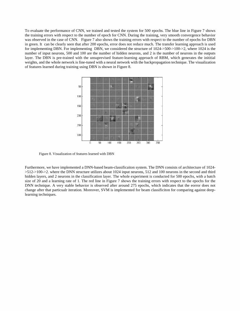
layer. The DBN is pre-trained with the unsuprevised feature-learning approach of RBM, which generates the inititial

weights, and the whole network is fine-tuned with a neural network with the backpropagation technique. The visualization

of features learned during training using DBN is shown in Figure 8.

Figure 8. Visualization of features learned with DBN

Furthermore, we have implemented a DNN-based beam-classificaiton system. The DNN consists of architecture of 1024-

>512->100->2. where the DNN structure utilizes about 1024 input neurons, 512 and 100 neurons in the second and third

hidden layers, and 2 neurons in the classification layer. The whole experiment is conducted for 500 epochs, with a batch

size of 20 and a learning rate of 1. The red line in Figure 7 shows the training errors with respect to the epochs for the

DNN technique. A very stable behavior is observed after around 275 epochs, which indicates that the eorror does not

change after that particualr iteration. Moreover, SVM is implemented for beam classificiton for comparing against deep-

learning techniques.

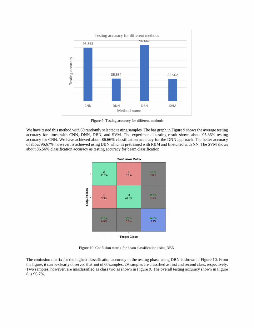
Figure 9. Testing accuracy for different methods

We have tested this method with 60 randomly selected testing samples. The bar graph in Figure 9 shows the average testing

accuracy for times with CNN, DNN, DBN, and SVM. The experimental testing result shows about 95.86% testing

accuracy for CNN. We have achieved about 86.66% classification accuracy for the DNN approach. The better accuracy

of about 96.67%, however, is achieved using DBN which is pretrained with RBM and finetuned with NN. The SVM shows

about 86.56% classification accuracy as testing accuracy for beam classification.

Figure 10. Confusion matrix for beam classification using DBN.

The confusion matrix for the highest classification accuracy in the testing phase using DBN is shown in Figure 10. From

the figure, it can be clearly observed that out of 60 samples, 29 samples are classified as first and second class, respectively.

Two samples, however, are misclassified as class two as shown in Figure 9. The overall testing accuracy shown in Figure

8 is 96.7%.

95.862

86.664

96.667

86.562

CNN DNN DBN SVM

Test

ing

accu

racy

Method name

Testing accuracy for different methods

Figure 11. Misclassified images: actual class one, classified as class two

4.3 Introspection

Deep learning is a data-driven learning approach. Due to the small number of training and testing samples, the deep

learning approach provided reasonable recognition accuracy. If the number of training samples is increased, however, the

deep-learning-based approaches will provide even better accuracy compared to any traditional machine-learning

approaches. Another comparison with feature-learning-based approaches is that the CNN has multiple layers of feature

extraction and selection in multiple levels. The second feature extraction layer (convolution and subsampling) combines

multiple features from the first layer and aggregates them into a more complex feature relationship layer. The final

completely connected layers make class decisions by combining sets of second-layer features.

5. CONCLUSION

In this work, we have implemented different deep learning techniques for classification of composite optical laser beams.

The experimental results show 95.86%, 86.66%, 96.67%, and 86.56% testing accuracy using CNN, DNN, DBN and SVM,

respectively. The best classification accuracy is observed using Deep Belief Network (DBN) methods compared to other

techniques. In the future, we would like to implement this solution with a transfer-learning approach [17]. In addition, we

would like to implement this problem on a Neuromorphic system called IBM’s TrueNorth system [18].

6. ACKNOWLEDGEMENT

The authors AASA and ZA will like to acknowledge the help of Judy Liebman, Lisa Belk and Sylwia Hamilton, for

constructive feedback and improving the readability of this article significantly. This work performed under the auspices

of the U.S. Department of Energy by Lawrence Livermore National Laboratory under Contract DE-AC52-07NA27344.

This paper is released as LLNL-CONF-737645.

REFERENCES

[1] Mark Bowers, Jeff Wisoff, Mark Herrmann, Tom Anklam, Jay Dawson, Jean-Michel Di Nicola, Constantin Haefner,

Mark Hermann, Doug Larson, Chris Marshall, Bruno Van Wonterghem and Paul Wegner, “Status of NIF laser and

high-power laser research at LLNL,” Proceedings Volume 10084, High Power Lasers for Fusion Research IV;

1008403 (2017)

[2] Mary L. Spaeth, Kenneth R. Manes, M. Bowers, P. Celliers, J.-M. Di Nicola, P. Di Nicola, S. Dixit, G. Erbert, J.

Heebner, D. Kalantar, O. Landen, B. MacGowan, B. Van Wonterghem, P. Wegner, C. Widmayer & S. Yang,

“National Ignition Facility Laser System Performance,” Fusion Science and Technology Vol. 69, 366-394 (2016).

[3] C. Haefner, J. E. Heebner, J. Dawson, S. Fochs, M. Shverdin, J.K. Crane, K. V. Kanz, J. Halpin, H. Phan, R.

Sigurdsson, W. Brewer, J. Britten, G. Brunton, B. Clark, M. J. Messerly, J. D. Nissen, B. Shaw, R. Hackel, M.

Hermann, G. Tietbohl, C. W. Siders and C.P.J. Barty, “Performance Measurement of the Injection Laser System

Configured for Picosecond Scale Advanced Radiographic Capability,” The Sixth International Conference on Inertial

Fusion Sciences and Applications, Journal of Physics: Conference Series 244, 032005 (2010).

[4] J. R. Rygg, O. S. Jones, J. E. Field, M. A. Barrios, L. R. Benedetti, G. W. Collins, D. C. Eder, M. J. Edwards, J. L.

Kline, J. J. Kroll, O. L. Landen, T. Ma, A. Pak, J. L. Peterson, K. Raman, R. P. Town, D. K. Bradley, “2D X-ray

radiography of imploding capsules at the national ignition facility,” Phys Rev Lett., 112, p. 195001 (2014).

[5] Richard Leach, Abdul A. Awwal, Roger Lowe-Webb, Victoria Miller-Kamm, Charles Orth, Randy Roberts, Karl

Wilhelmsen, “Image processing for the Advanced Radiographic Capability (ARC) at the National Ignition Facility,”

Proc. SPIE. 9970, Optics and Photonics for Information Processing X, p 99700M (2016).

[6] A. A. S. Awwal, K. Wilhelmsen, R. R. Leach, V. Miller-Kamm, S. Burkhart, R. Lowe-Webb, and S. Cohen,

“Autonomous monitoring of control hardware to predict off-normal conditions using NIF automatic alignment

systems,” Fusion Engineering and Design, Volume 87, 2140–2144 (2012).

[7] Y. LeCun, L. Bottou, Y. Bengio, and P. Haffner, “Gradient-based learning applied to document recognition,”

Proceedings of the IEEE, vol. 86, no. 11, pp. 2278–2324 (1998).

[8] Alex Krizhevsky, Ilya Sutskever, and Geoffrey E. Hinton. "Imagenet classification with deep convolutional neural

networks." Advances in neural information processing systems, Vol. 25, pp. 1097-1105 (2012).

[9] V. Nair and G. Hinton, “Rectified linear units improve restricted boltzmann machines,” Proceedings of the 27th

International Conference on Machine Learning (ICML-10), 807-814 (2010).

[10] Yichuan Tang “Deep Learning using Linear Support Vector Machines” proceedings of International Conference on

Machine Learning in 2013.

[11] Kunihiko Fukushima and Sei Miyake. "Neocognitron: A self-organizing neural network model for a mechanism of

visual pattern recognition." Competition and cooperation in neural nets. Springer, Berlin, Heidelberg, 267-285 (1982)

[12] Kaiming He, et al. "Delving deep into rectifiers: Surpassing human-level performance on imagenet

classification." Proceedings of the IEEE international conference on computer vision, pp. 1026-1034 (2015).

[13] Abdel-rahman Mohamed, George E. Dahl, and Geoffrey Hinton, “Acoustic modeling using deep belief networks,”

Audio, Speech, and Language Processing, IEEE Transactions on 20, 14-22 (2012)

[14] M. Welling, M. Rosen-Zvi, and G. E. Hinton, “Exponential family harmoniums with an application to information

retrieval,” in Proc. NIPS 17 (2004).

[15] A. K. Noulas and B.J.A. Kröse, “Deep Belief Networks for Dimensionality Reduction,” Belgian-Netherlands

Conference on Artificial Intelligence, pp. 185-191 (2008).

[16] L. McAfee, “Document Classification using Deep Belief Nets,” CS224n, Sprint 2008.

[17] G. Mesnil, Y. Dauphin, et al. "Unsupervised and transfer learning challenge: a deep learning approach." Proceedings

of ICML Workshop on Unsupervised and Transfer Learning, Vol. 27, pp. 97-111 (2012).

[18] Filipp Akopyan, et al. "Truenorth: Design and tool flow of a 65 mw 1 million neuron programmable neurosynaptic

chip." IEEE Transactions on Computer-Aided Design of Integrated Circuits and Systems 34 1537-1557 (2015)