EMU and Portfolio

Research Paper N° 31

FAME - International Center for Financial Asset Management and Engineering

THE GRADUATE INSTITUTE OFINTERNATIONAL STUDIES

40, Bd. du Pont d’ArvePO Box, 1211 Geneva 4

Switzerland Tel (++4122) 312 09 61 Fax (++4122) 312 10 26

http: //www.fame.ch E-mail: admin@fame.ch

April 2000

HEC-University of Lausanne, CEPR and FAME

Diversification

Jean-Pierre DANTHINE

OpportunitiesKpate ADJAOUTEMorgan Stanley Capital International, Geneva

INTERNATIONAL CENTER FOR FINANCIAL ASSET MANAGEMENT AND ENGINEERING 40 bd du Pont d'Arve • P.O. Box 3 • CH-1211 Geneva 4 • tel +41 22 / 312 0961 • fax +41 22 / 312 1026

http://www.fame.ch • e-mail: admin@fame.ch

RESEARCH PAPER SERIES The International Center for Financial Asset Management and Engineering (FAME) is a private foundation created in 1996 at the initiative of 21 leading partners of the finance and technology community together with three Universities of the Lake Geneva Region (Universities of Geneva, University of Lausanne and the Graduate Institute of International Studies). Fame is about research, doctoral training, and executive education with “interfacing” activities such as the FAME lectures, the Research Day/Annual Meeting, and the Research Paper Series. The FAME Research Paper Series includes three types of contributions: • First, it reports on the research carried out at FAME by students and research fellows. • Second, it includes research work contributed by Swiss academics and practitioners

interested in a wider dissemination of their ideas, in practitioners' circles in particular. • Finally, prominent international contributions of particular interest to our constituency are

included as well on a regular basis. FAME will strive to promote the research work in finance carried out in the three partner Universities. These papers are distributed with a ‘double’ identification: the FAME logo and the logo of the corresponding partner institution. With this policy, we want to underline the vital lifeline existing between FAME and the Universities, while simultaneously fostering a wider recognition of the strength of the academic community supporting FAME and enriching the Lemanic region. Each contribution is preceded by an Executive Summary of two to three pages explaining in non-technical terms the question asked, discussing its relevance and outlining the answer provided. We hope the series will be followed attentively by all academics and practitioners interested in the fields covered by our name. I am delighted to serve as coordinator of the FAME Research Paper Series. Please contact me if you are interested in submitting a paper or for all suggestions concerning this matter. Sincerely,

Prof. Martin Hoesli University of Geneva, HEC 40 bd du Pont d'Arve 1211 Genève 4 Tel: +41 (022) 705 8122 Martin.Hoesli@hec.unige.ch

EMU AND PORTFOLIO DIVERSIFICATION OPPORTUNITIES

Kpate ADJAOUTE Jean-Pierre DANTHINE

April 2000

1

EMU AND PORTFOLIO DIVERSIFICATION OPPORTUNITIES

Kpate Adjaouté Morgan Stanley Capital International (Geneva)

and

Jean-Pierre Danthine University of Lausanne, CEPR and FAME

April 2000

Note: The present text reports on part of the research carried on under mandate from the European Commission – Danthine J.P., K. Adjaouté, L. Bottazzi, A. Fischer, R. Hamaui, R.Portes and M. Wickens, “EMU and Portfolio Adjustment”, CEPR report for the European Commission, mimeo 112 pp, December 1999 – and summarized in EMU and Portfolio Adjustment , CEPR Policy Paper N° 5, November 2000. We thank our co-authors and Vihang Errunza for their comments as well as Agim Xhaja for excellent research assistance.

Abstract This paper studies the impact of EMU on portfolio diversification opportunities. We find a significant increase in the correlation between stock returns, whether they are computed on the basis of market or sector indices. This is true for two definitions of the pre-convergence and convergence periods. Diversification opportunities within the Euro-area have thus been reduced. The culprit appears to be less the disappearance of currency risk than the convergence of economic structures and/or the homogenisation of economic shocks (across the Euro-15 member states). This evolution should mark the end of pure country allocation strategies within Europe. If these are the alternatives, the increased conformity of stock returns implies that international diversification does not pay: the cost of the home bias within Euroland has been lowered (in some cases to zero). Diversification across both countries and sectors, however, remains the much superior investment strategy, and, in light of this option, the cost of the home bias continues to be significant. JEL codes: F30;G11;G15 Key words: EMU, portfolio diversification, home bias

2

Executive Summary This paper studies the impact of EMU on portfolio diversification opportunities. We focus on equity markets and understand under the label ‘EMU’ the entire economic and monetary integration process at work in Euro-land in the 90’s culminating with the advent of the Euro on January 1, 1999. International diversification is performance improving to the extent that national stock markets of the Euro area are imperfectly correlated. The advent of the Euro has at least two possible implications in this respect. First, it corresponds mechanically to the disappearance of currency risks, and second, it is part of a broader set of structural changes likely to alter the traditional forces underlying asset returns and thus, the relevant correlations between stock indices. To shed light on these issues and their implications for portfolio allocation decisions, we focus on the evolving characteristics of the variance-covariance matrix of returns within Euro-land. The question we address is the following: have we observed significant changes, over the recent past, as the monetary and economic convergence process was unfolding (and with the advent of the Euro), in the characteristics of returns? And, if so, what are their implications for optimal portfolio allocations? We find indeed that the conditions under which portfolio investors diversify across the Euro-area equity markets have changed materially in the 1990s. With an increased degree of correlation between either national stock indices, diversification opportunities have been significantly reduced. It seems difficult not to incriminate the process of economic and monetary integration process at work in Europe during this period for this result. Within this process, however, the disappearance of currency risk is decidedly less important for investors than the convergence of economic structures and/or the homogenisation of economic shocks (across the Euro-15 member states). That is, the increased stock return correlations are as manifest when we abstract from currency fluctuations than when they are computed using effective monetary returns. As a consequence of these changes, we wonder whether the evolution of return correlations at the country level would justify abandoning the traditional country allocation model in favour of an approach based on a diversification across industrial sectors. To get an insight into this question, the time evolution of the variance-covariance matrices of sectoral returns is also studied. Two disaggregation levels are considered: at a first level, four sectors per country are considered, and at the second level, 10 sectors are taken into account.

Our finding is that indeed this evolution should mark the end of pure country allocation strategies within Europe: the increased conformity of stock returns implies that international diversification across the Euro-area on the basis of a pure country allocation model has increasingly smaller benefits.

This result has implications for the celebrated ‘home bias’, the propensity of most investors to invest disproportionately in their home market. Our results suggest that the changing economic structures within Europe and the disappearance of currency risks may have lowered the cost of the home bias within Euroland. This intuition is confirmed if the alternative to staying at home is to diversify with the use of a pure country

3

allocation model. In some cases, the cost of the home bias thus understood has decreased to zero.

Further analysis however shows that diversification across both countries and sectors, remains the much superior investment strategy and that, in light of this option, the cost of the home bias continues to be significant in Europe.

4

1. Introduction This paper studies the impact of EMU on portfolio diversification opportunities. We focus on equity markets and understand under the label ‘EMU’ the entire economic and monetary integration process at work in Euro-land in the 90’s. In this context, international diversification is performance improving to the extent that national stock markets of the Euro area are imperfectly correlated. The advent of the Euro has at least two possible implications in this respect. First, it corresponds mechanically to the disappearance of currency risks, and second, it is part of a broader set of structural changes likely to alter the traditional forces underlying asset returns and thus, the relevant correlations between stock indices. To shed light on these issues and their implications for portfolio allocation decisions, we start by focusing on the characteristics of the variance-covariance matrix of returns within Euro-land. The question we address is the following: have we observed significant changes, over the recent past, as the monetary and economic convergence process was unfolding (and with the advent of the Euro), in the characteristics of returns? And, if so, what are their implications for optimal portfolio allocations? A closely related issue is whether the evolution of return correlations at the country level would justify abandoning the traditional country allocation model in favour of an approach based on a diversification across industrial sectors. To get an insight into this question, the time evolution of the variance-covariance matrices of sectoral returns is also studied. Two disaggregation levels are considered: at a first level, four sectors per country are considered, and at the second level, 10 sectors are taken into account.

Finally, given the persistence and the importance of the home bias in equity investments, the paper pursues with the following question: do the changing economic structures within Europe and the disappearance of currency risks tend to increase or decrease the cost of restricting one’s investment universe to home equities?

2. The Data

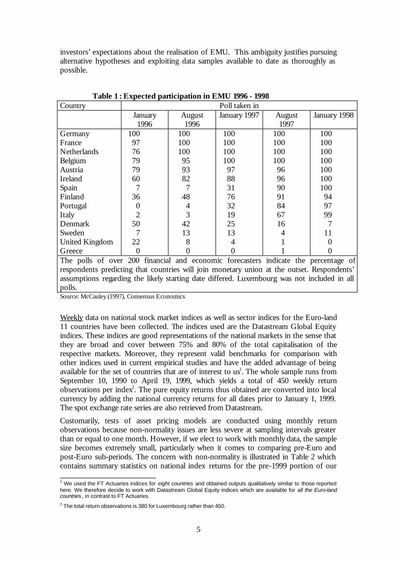
For the purpose of comparison, we need pre-Euro and post-Euro periods. Given the relatively short post-Euro period, the available data constitute a severe hindrance. To bypass the difficulty, the problem is approached from two perspectives, both making the assumption that January 1st 1999 was but the final consecration of a movement of convergence started earlier. Our first, stronger, hypothesis is that the start of the convergence period may be identified with January 1995, the date of entry of the Maastricht Treaty. This enables the use the period from September 1990 to the end of 1994 as representative of the ‘pre-convergence’ period and to make full use of the data sample available. A more realistic hypothesis is to use the information provided by opinion polls. In fact, while one may argue that the prospects of a monetary union were surrounded with considerable uncertainty in January 1995, this uncertainty for most participating countries was resolved much ahead of the starting date of January 1999. Indeed, Table 1 indicates that for Germany, France, Netherlands, Belgium and Austria, the prospects of EMU were close to certainty as early as August 1996; by August 1997, only for Italy were there some doubts which were lifted by January 1998. The ambiguity over the exact date of the convergence period is inevitable, since it is linked with private

5

investors’ expectations about the realisation of EMU. This ambiguity justifies pursuing alternative hypotheses and exploiting data samples available to date as thoroughly as possible.

Table 1 : Expected participation in EMU 1996 - 1998 Country Poll taken in January

1996 August 1996

January 1997 August 1997

January 1998

Germany France Netherlands Belgium Austria Ireland Spain Finland Portugal Italy Denmark Sweden United Kingdom Greece

100 97 76 79 79 60 7

36 0 2

50 7

22 0

100 100 100 95 93 82 7

48 4 3

42 13 8 0

100 100 100 100 97 88 31 76 32 19 25 13 4 0

100 100 100 100 96 96 90 91 84 67 16 4 1 1

100 100 100 100 100 100 100 94 97 99 7

11 0 0

The polls of over 200 financial and economic forecasters indicate the percentage of respondents predicting that countries will join monetary union at the outset. Respondents’ assumptions regarding the likely starting date differed. Luxembourg was not included in all polls. Source: McCauley (1997), Consensus Economics

Weekly data on national stock market indices as well as sector indices for the Euro-land 11 countries have been collected. The indices used are the Datastream Global Equity indices. These indices are good representations of the national markets in the sense that they are broad and cover between 75% and 80% of the total capitalisation of the respective markets. Moreover, they represent valid benchmarks for comparison with other indices used in current empirical studies and have the added advantage of being available for the set of countries that are of interest to us1. The whole sample runs from September 10, 1990 to April 19, 1999, which yields a total of 450 weekly return observations per index2. The pure equity returns thus obtained are converted into local currency by adding the national currency returns for all dates prior to January 1, 1999. The spot exchange rate series are also retrieved from Datastream.

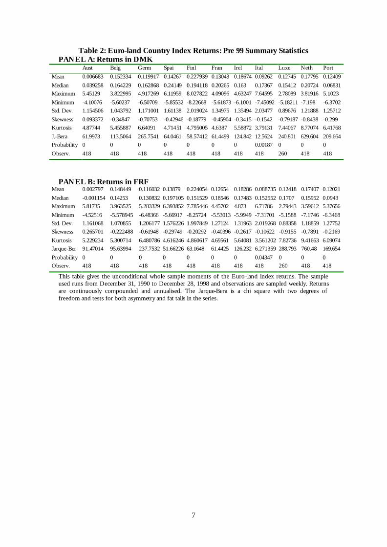
Customarily, tests of asset pricing models are conducted using monthly return observations because non-normality issues are less severe at sampling intervals greater than or equal to one month. However, if we elect to work with monthly data, the sample size becomes extremely small, particularly when it comes to comparing pre-Euro and post-Euro sub-periods. The concern with non-normality is illustrated in Table 2 which contains summary statistics on national index returns for the pre-1999 portion of our 1 We used the FT Actuaries indices for eight countries and obtained outputs qualitatively similar to those reported here. We therefore decide to work with Datastream Global Equity indices which are available for all the Euro-land countries , in contrast to FT Actuaries. 2 The total return observations is 380 for Luxembourg rather than 450.

6

sample. As will be done systematically, we illustrate our arguments by taking the viewpoints of the German and French investors. Based on the Jarque-Bera statistic (which is a chi square with two degrees of freedom), the normality assumption is rejected for all 11 countries and both types of investors. The normality is rejected both because of fat tails and asymmetry as indicated by the kurtosis and skewness coefficients. In fact,

given that the kurtosis coefficient

→T

Nk24

,3 and the skewness

→T

Ns6

,0 ,

and that the Jarque-Bera is a combination of the latter two statistics, it is easy to see that asymmetry is present in all but three stock returns (Austria, Finland and Italy) when we focus on returns expressed in DMK. With no exception, index returns are characterised by fat tails. Belgium, Finland and Italy exhibit asymmetry when returns are expressed in FRF and fait tails are present for all countries.

The main question here is to figure out the likely consequences of this non-normality on the battery of tests that are going to be undertaken in this study. Given the evidence of fat tails, the primary message is that sample second moments are unreliable estimates of the true population moments, which might not even exist3. The very simple and conservative assumption that is maintained here is that the general form of the underlying return distribution (whatever it is) does not change significantly over the time period of our study, so that correlation and covariance matrices computed over two consecutive sub-periods can be viewed as coming from the same distribution.

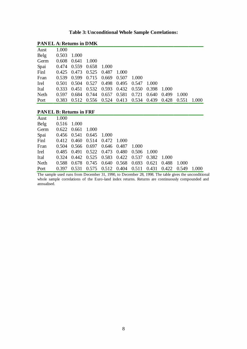
Table 3 reports the unconditional correlations obtained for the pre-1999 part of our sample.

3 Fat tails suggest that returns can be modelled by stable paretian distributions which can have infinite second moments.

7

Table 2: Euro-land Country Index Returns: Pre 99 Summary Statistics PANEL A: Returns in DMK

Aust Belg Germ Spai Finl Fran Irel Ital Luxe Neth Port Mean 0.006683 0.152334 0.119917 0.14267 0.227939 0.13043 0.18674 0.09262 0.12745 0.17795 0.12409 Median 0.039258 0.164229 0.162868 0.24149 0.194118 0.20265 0.163 0.17367 0.15412 0.20724 0.06831 Maximum 5.45129 3.822995 4.917269 6.11959 8.027822 4.09096 4.63247 7.64595 2.78089 3.81916 5.1023 Minimum -4.10076 -5.60237 -6.50709 -5.85532 -8.22668 -5.61873 -6.1001 -7.45092 -5.18211 -7.198 -6.3702 Std. Dev. 1.154506 1.043792 1.171001 1.61138 2.019024 1.34975 1.35494 2.03477 0.89676 1.21888 1.25712 Skewness 0.093372 -0.34847 -0.70753 -0.42946 -0.18779 -0.45904 -0.3415 -0.1542 -0.79187 -0.8438 -0.299 Kurtosis 4.87744 5.455887 6.64091 4.71451 4.795005 4.6387 5.58872 3.79131 7.44067 8.77074 6.41768 J.-Bera 61.9973 113.5064 265.7541 64.0461 58.57412 61.4499 124.842 12.5624 240.801 629.604 209.664 Probability 0 0 0 0 0 0 0 0.00187 0 0 0 Observ. 418 418 418 418 418 418 418 418 260 418 418

PANEL B: Returns in FRF

Mean 0.002797 0.148449 0.116032 0.13879 0.224054 0.12654 0.18286 0.088735 0.12418 0.17407 0.12021 Median -0.001154 0.14253 0.130832 0.197105 0.151529 0.18546 0.17483 0.152552 0.1707 0.15952 0.0943 Maximum 5.81735 3.963525 5.283329 6.393852 7.785446 4.45702 4.873 6.71786 2.79443 3.59612 5.37656 Minimum -4.52516 -5.578945 -6.48366 -5.66917 -8.25724 -5.53013 -5.9949 -7.31701 -5.1588 -7.1746 -6.3468 Std. Dev. 1.161068 1.070855 1.206177 1.576226 1.997849 1.27124 1.31963 2.019268 0.88358 1.18859 1.27752 Skewness 0.265701 -0.222488 -0.61948 -0.29749 -0.20292 -0.40396 -0.2617 -0.10622 -0.9155 -0.7891 -0.2169 Kurtosis 5.229234 5.300714 6.480786 4.616246 4.860617 4.69561 5.64081 3.561202 7.82736 9.41663 6.09074 Jarque-Ber 91.47014 95.63994 237.7532 51.66226 63.1648 61.4425 126.232 6.271359 288.793 760.48 169.654 Probability 0 0 0 0 0 0 0 0.04347 0 0 0 Observ. 418 418 418 418 418 418 418 418 260 418 418

This table gives the unconditional whole sample moments of the Euro-land index returns. The sample used runs from December 31, 1990 to December 28, 1998 and observations are sampled weekly. Returns are continuously compounded and annualised. The Jarque-Bera is a chi square with two degrees of freedom and tests for both asymmetry and fat tails in the series.

8

Table 3: Unconditional Whole Sample Correlations: PANEL A: Returns in DMK Aust 1.000 Belg 0.503 1.000 Germ 0.608 0.641 1.000 Spai 0.474 0.559 0.658 1.000 Finl 0.425 0.473 0.525 0.487 1.000 Fran 0.539 0.599 0.715 0.669 0.507 1.000 Irel 0.501 0.504 0.527 0.498 0.495 0.547 1.000 Ital 0.333 0.451 0.532 0.593 0.432 0.550 0.398 1.000 Neth 0.597 0.684 0.744 0.657 0.581 0.721 0.640 0.499 1.000 Port 0.383 0.512 0.556 0.524 0.413 0.534 0.439 0.428 0.551 1.000 PANEL B: Returns in FRF Aust 1.000 Belg 0.516 1.000 Germ 0.622 0.661 1.000 Spai 0.456 0.541 0.645 1.000 Finl 0.412 0.460 0.514 0.472 1.000 Fran 0.504 0.566 0.697 0.646 0.487 1.000 Irel 0.485 0.491 0.522 0.473 0.480 0.506 1.000 Ital 0.324 0.442 0.525 0.583 0.422 0.537 0.382 1.000 Neth 0.588 0.678 0.745 0.640 0.568 0.693 0.621 0.488 1.000 Port 0.397 0.531 0.575 0.512 0.404 0.511 0.431 0.422 0.549 1.000 The sample used runs from December 31, 1990, to December 28, 1998. The table gives the unconditional whole sample correlations of the Euro-land index returns. Returns are continuously compounded and annualised.

9

3. Statistical Analysis of Correlation and Variance-Covariance Matrices of Returns Based on Country Indices

To assess the extent to which the adoption of a common policy in the convergence phase has led to a significant modification of the investment opportunities within Euro-land, the whole sample is partitioned into two sub-samples of equal size. In a first approach, the first sub-sample runs from December 31, 1990 to December 26, 1994 and corresponds to the four years preceding the starting date of the Maastricht Treaty. The second sub-sample runs from January 2, 1995 to December 28, 1998 and corresponds to the first definition of the convergence period. Section 4 presents the corresponding results for a more restricted definition of the convergence period.

The modification of the investment opportunity set, if any, must manifest itself in the changing structure of the variance-covariance matrices of the pre convergence and convergence periods. In principle, a test of the stability of the covariance matrices can suffice. But given that correlation matrices are more appropriate to judge on the significance of international diversification benefits, we will consider tests of stability of both correlation and covariance matrices. The tests that are used are the Jenrich [1970] and Box [1949] 2χ statistics which have been used in a number of empirical studies (Longin and Solnik [1995], Kaplanis [1985, 1988] to cite a few). Operationally, denote by vm1 and vm 2 the variance-covariance matrices of the first sub-sample (pre-convergence) and second sub-sample (convergence), respectively. The corresponding correlation matrices are denoted by cm1 and cm 2 respectively. For a test based on covariance matrices, the Box test is based on a ratio of determinants:

vvvv mmmm 2121 / ++ , while the Jenrich uses as its principal input the quantity ( ) ( )vvvv mmmmtrace 2121 / +− . The null hypothesis to be tested through the Jenrich

statistic when covariance matrices are involved is vvv mmm == 21 . When correlation matrices are considered instead, the null hypothesis evaluated is ccc mmm == 21 . To focus on tests of equality of correlation matrices first, we define:

( ) ( ) ( )ijccc rTTmTmTm =++= 212211 / = “average” correlation matrix , where 1T and

2T represent the relevant sample sizes.

ijδ = Kronecker delta = identity matrix of the same dimension as cm .

+=

ijijij rrS δ

( )ccc mmmTT

TTZ 21

12/1

21

21 −

+

=−

The Jenrich test statistic can then finally be computed as:

( ) ( ) ( )ZdgSZdgZtr 122 '21 −−=χ

This test statistic is a chi square with degrees of freedom equal to ( )2

1−nn where n is the

number of assets (or countries).

For a test of stability of covariance matrices, the test statistic is computed in exactly the same way as the test for stability of correlation matrices, after making appropriate substitutions (replacing correlation matrices by covariance matrices) and

10

adjusting for the number of degrees of freedom. When we replace the correlation matrices with the corresponding covariance matrices, the appropriate test statistic then becomes:

( )22

21

Ztr=χ

The number of degrees of freedom in that case is ( )2

1+nn . It thus appears that

the number of degrees of freedom is lower in the correlation case, because the diagonal elements of the correlation matrices are not an object of test. Hence, the second term in the statistic for testing the equality of correlation matrices can be viewed as a correction term, since the comparison of correlation matrices involves a lower degree of freedom

( ( )2

1−nn ). To summarise, in the context of the present study involving 11 countries, the

Box and Jenrich statistics based on covariance matrices have 66 degrees of freedom whereas the Jenrich statistic using correlation matrices has 55 degrees of freedom. For practical reasons, Luxembourg is excluded from our sample and we adjust the degrees of freedoms accordingly.

The small sample properties of both tests have been investigated by Kaplanis [1985]. It turns out that if the sample size is too small, the two tests can give conflicting conclusions. Hence, the use of both tests here can give guidance on possible sample issues. The output of the calculations is reported in Table 4 below. Table 4 : Test of Stability of Covariance and Correlation Matrices When Returns

Are Expressed in DMK and in FRF

Test of Corr. Matrices Test of Cov. Matrices Jenrich Jenrich Returns in DMK 171.752 231.681 (0.0000) (0.0000) Returns in FRF 172.259 230.489 (0.0000) (0.0000) When we focus on pre convergence vs. convergence periods, the first sub-sample runs from December 31, 1990 to December 26, 1994 while the second sub-sample runs from January 2, 1995 to December 28, 1998. The p-values are given in parentheses below each statistic. Clearly, there is a strong evidence that both the correlation and variance-covariance matrices are unstable over time. The extremely low p-values given in parentheses reject the null hypothesis of equality of the two matrices, implying that the diversification benefits during the convergence period are different from those prevailing in the period before convergence. Additional information is presented in Figures 1 and 2 where we display the pre-convergence and convergence period country pair correlations. (The corresponding numerical figures are reported in Tables D and E in the Appendix) The pre-convergence correlations are sorted in ascending order, and plotted along with the unsorted corresponding convergence period correlations. It is striking that every convergence period correlation is higher (with 3 or 4 exceptions when returns are

11

expressed in DMK or FRF respectively) than its pre-convergence period counterpart. The formal Jenrich tests confirm that these differences are statistically significant.

Of course, it is a relevant question to inquire whether this pattern of increasing return correlations is specific to Euro-land countries and thus, presumably, associated with the process of economic and monetary unification, or whether it is merely a reflection of a broader world wide trend, possibly as a consequence of increasingly mobile international capital flows. Evidence on this question is provided in Figure 3 where we display the evolution of the return correlations between stock indices representing the major regions of the world. The regions that are considered here are: Americas (AM), Far East (FE), Pacific-Basin (PB), Australasia (AU), Non-European Union (NE), European Union (EE) and Asia (AS). While there is some increase in the level of correlations as the data in the Appendix (Table C) suggest, the changes in correlations are significantly more pronounced in the case of Euro-land countries (the average of region pair correlations was 0.454 during the pre convergence period, and it moved to only 0.585 during the convergence period)4. In addition, with the exception of the correlations involving the Far East and Pacific Basin regions, the level of correlations tend to be lower than those observed within Euro-land.

Table 5 indicates that these changes in correlations were accompanied by an increase in the standard deviations of returns across Europe, with Italy being the sole exception and the Netherlands the extreme illustration. While it is easy to find some rationale for the increase in correlations (see section 8), it is not clear that the increase in the risk level has any causal relationship with EMU or the process of European economic integration, and it is difficult to decide whether this increase in standard deviations is likely to be permanent or not. It is interesting to notice however, that there is some presumption that return correlations increase during periods of high volatility (e.g., see the contagion literature). The increase in the standard deviations in returns may in this sense explain part of the common increase in correlations both in Euro-land and elsewhere in the developed world.

The intermediate conclusion to draw from the analysis of this section is that the process of economic and monetary integration in place in Europe seems to be accompanied with an increase in the correlation of national stock indices indicating that the benefits of international diversification using country allocation models within Euro-land have diminished. A similar but less pronounced process of increasing correlations among country or regional indices is manifest elsewhere in the world, suggesting that EMU factors are not the only ones at work. It remains true that diversification opportunities on a purely geographical basis are better if extended outside the European region.

4 Contrast this with an average pre convergence correlation of 0.333 and a convergence period average correlation of 0.585 for Euro-land countries.

12

Table 5: Return Volatilities in Euro-land

Country Pre-Conv. Converg. Neth. 0.7306081 1.39186 Belg. 0.7774509 1.114882 Germ. 0.9380667 1.286281 Port. 0.9956962 1.376585 Aust. 1.0016007 1.027208 Irel. 1.1253629 1.268636 Fran. 1.1486571 1.355324 Spai. 1.3931264 1.565336 Finl. 1.7876227 1.972845 Ital. 1.815288 1.796955

Figure 1

Evolution of Country Pair Correlations (Returns in Marks): Before and During Convergence

-0.2

0

0.2

0.4

0.6

0.8

1

It-L

u

Ir-It

Fi-L

u

Be-I

t

Fi-I

t

Sp-I

r

Au-

Sp

Fi-P

o

Fr-P

o

Ge-

Ir

Au-

Fr

Sp-F

i

Ge-

It

Fr-I

r

Be-S

p

Au-

Ir

Be-

Ge

Be-

Ne

Ge-

Ne

Country Pairs

Cor

rela

tions

Pre-Conv.

Converg.

13

Figure 2

Evolution of Country Pair Correlations (Returns in FRF): Before and During Convergence

-0.4

-0.2

0

0.2

0.4

0.6

0.8

1It

-Lu

Ir-I

t

Fi-L

u

Be-I

t

Fi-I

t

Au-

Sp

Be-P

o

Fi-P

o

It-N

e

Au-

Fr

Fi-F

r

Be-L

u

Ir-L

u

Be-S

p

Au-

Be

Be-I

r

Be-F

r

Be-G

e

Ge-

Ne

Country Pairs

Cor

rela

tions

Pre-Conv.

Converg.

Figure 3

Evolution of Region Pair Correlations: Before and During Convergence

0

0.2

0.4

0.6

0.8

1

1.2

AM-FEAM-AS

AM-PBAU-NE

AU-FEAS-A

UAU-PB

AU-EE

AM-AUFE

-NE

AM-NEAS-N

ENE-P

BAM-EE

EE-FEAS-E

EEE-PB

EE-NEFE

-PBAS-F

EAS-P

B

Region Pairs

Cor

rela

tions

Pre-Conv.Converg.

14

4. A More Cautious Definition of the Convergence Period.

In this section, the analysis above is revisited using the ‘Consensus Economics’ definition of the convergence period. On the basis of the information provided in Table 1, we date the start of the convergence period at August 1997 (extending until the end of our data sample, i.e. April 19, 1999) and accordingly, define a pre-convergence period of same length, i.e. starting on November 13, 1995.

Table 6 reports the return correlations obtained for the pre-convergence and convergence periods for both types of investors. The results strikingly confirm what was obtained with the first sample decomposition. Whether returns are computed in DMK or FRF, only two of the 45 correlations are lower in the convergence period than in the pre-convergence one! Not surprisingly, Table 7 confirms that the pre-convergence and convergence covariance and correlation matrices differ significantly.

Thus, even with a narrower definition of the convergence period, the data send the same message. The recent years, associated with increasing economic integration in Europe culminating with EMU, have seen an increase in the equity return correlations confronting European investors with reduced diversification opportunities. An important question is whether these changes are an (almost) mechanical consequence of decreasing currency risk (which altogether disappeared in the latter part of our sample) or whether they rather reflect underlying changes in the ‘real’ structures of economies engaged in a process of monetary and economic integration. Some insight into this question is provided by repeating the previous exercise in a context where currency fluctuations prior to January 1, 1999 have been neutralised.

Table 6: Correlations Based on Consensus Economics Periods PANEL A: Pre Convergence, Returns in DMK Aust 1 Belg 0.63 1 Germ 0.58 0.575 Spai 0.39 0.478 0.51 1 Finl 0.4 0.376 0.489 0.37 1 Fran 0.38 0.549 0.61 0.43 0.3451 1 Irel 0.46 0.521 0.528 0.38 0.3219 0.541 1 Ital 0.33 0.512 0.326 0.37 0.3905 0.479 0.3799 Neth 0.56 0.663 0.778 0.58 0.4533 0.586 0.6041 0.3788 1 Port 0.27 0.426 0.471 0.41 0.3729 0.393 0.3225 0.3457 0.4435 1

15

PANEL B: Convergence Period, Returns in DMK Aust 1 Belg 0.55 1 Germ 0.66 0.822 1 Spai 0.62 0.745 0.834 1 Finl 0.68 0.665 0.815 0.73 1 Fran 0.73 0.801 0.907 0.83 0.7992 1 Irel 0.59 0.501 0.639 0.56 0.6688 0.596 1 Ital 0.53 0.692 0.76 0.85 0.6894 0.813 0.5075 1 Neth 0.7 0.809 0.902 0.82 0.8281 0.911 0.6661 0.7671 1 Port 0.59 0.694 0.753 0.75 0.6053 0.779 0.5013 0.7298 0.745 1 PANEL C: Pre Convergence, Returns in FRF Aust 1 Belg 0.63 1 Germ 0.61 0.586 1 Spai 0.38 0.464 0.501 1 Finl 0.44 0.405 0.518 0.38 1 Fran 0.35 0.518 0.586 0.4 0.3532 1 Irel 0.46 0.511 0.53 0.36 0.3463 0.506 1 Ital 0.3 0.485 0.3 0.35 0.3888 0.452 0.3486 1 Neth 0.56 0.658 0.775 0.57 0.4726 0.564 0.5946 0.3538 1 Port 0.3 0.441 0.495 0.4 0.401 0.376 0.3282 0.3268 0.4493 1 PANEL D: Convergence, Returns in FRF Aust 1 Belg 0.57 1 Germ 0.67 0.825 1 Spai 0.62 0.746 0.834 1 Finl 0.66 0.658 0.81 0.72 1 Fran 0.73 0.803 0.907 0.83 0.7947 1 Irel 0.58 0.497 0.633 0.56 0.663 0.586 1 Ital 0.55 0.699 0.765 0.85 0.6882 0.818 0.5084 1 Neth 0.69 0.806 0.901 0.82 0.8253 0.91 0.6588 0.77 1 Port 0.6 0.699 0.755 0.75 0.6011 0.781 0.4952 0.7344 0.7443 1

The Pre Convergence period based on Consensus Economics runs from November 13, 1995 to July 28, 1997 whereas the Convergence Period runs from August 4, 1997 to April 19, 1999.

16

Table 7 : Test of Stability of Covariance and Correlation Matrices When Returns Are Expressed in DMK and in FRF (Consensus Economics)

Test of Corr. Matrices Test of Cov. Matrices Jenrich Jenrich Returns in DMK 92.971 198.125 (0.00003) (0.00000) Returns in FRF 92.476 197.148 (0.00004) (0.0000)

The Pre Convergence period based on Consensus Economics runs from November 13, 1995 to July 28, 1997 whereas the Convergence Period runs from August 4, 1997 to April 19, 1999. 5. Taking the Viewpoint of the Euro- Investor

Given the evidence reported in the previous sections, the rest of the analysis will abstract from currency risk and concentrate on the implications for diversification benefits of the changes in economic structures associated with EMU. While the argument can be made that currency fluctuations within the Euro area have been significant in the years before full convergence, the impact of these fluctuations do not seem to be visible in a portfolio diversification context (offsetting effects). Hence, the single viewpoint of the European investor is adopted; this is appropriate post January 1, 1999 and return data are expressed in Euro at single conversion rates: the official, permanent conversion rates of December 31st 1998. That is, we convert all national and sector indices in Euro at the December 31st 1998 conversion rates, also for index values preceding the formal advent of EMU and compute our returns on that basis. The implicit underlying hypothesis is that the currency exchange rate movements since 1990 have been mostly neutral to stock returns and that the main measurable effect of the advent of the Euro is not so much the result of the disappearance of currency risks but rather follows the changes in economic structure that the process of economic and monetary unification has provoked. The justification for this choice can be debated in relation to currency variations shown in the Appendix (Table F). We will indeed show that, as far as our analysis is concerned, currency fluctuations have played a minor role in the 1990’s (in Europe). That is, the result of the two preceding sections will be fully confirmed in the hypothetical context of this section, suggesting that the increase in return correlations measured in the preceding subsections may be due, to a greater extent, to the evolving economic structure rather than to the simple elimination of currency risk. If this is so, one may conjecture that the described evolution may not have terminated its course with the arrival of the single currency.

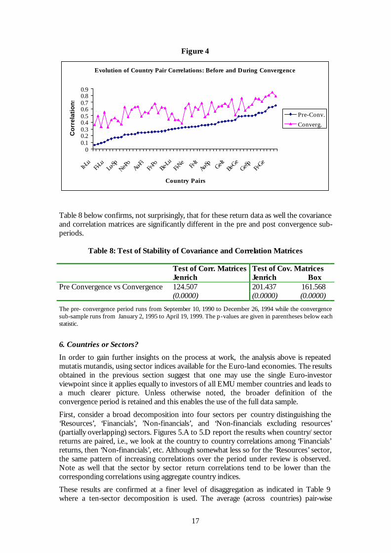
Turning to the full sample and using the broader definition of convergence period mentioned in section 2, Figure 4 corresponds to Figures 1 and 2 for the return data ‘purged’ from currency fluctuations (where consequently, the single viewpoint of the Euro-investor is relevant). The upward shift in the correlation matrix is clearly visible, confirming the decrease in international diversification benefits. If the convergence period is further decomposed in two sub-periods, it is also found that the correlations of the second period of convergence are much higher than those of the first phase (results not reported here). Thus, not only have correlations increased between pre convergence and post convergence, but they also continue to do so during the post convergence period!

17

Figure 4

Evolution of Country Pair Correlations: Before and During Convergence

00.10.20.30.40.50.60.70.80.9

It-Lu

Fi-Lu

Lu-Sp

Ne-Po

Au-Fi

Fr-Po

Be-Lu

Fi-Ne

Fr-It

Au-Sp

Ge-ItBe-

GeGe-Sp Fr-

Ge

Country Pairs

Co

rrel

atio

ns

Pre-Conv.

Converg.

Table 8 below confirms, not surprisingly, that for these return data as well the covariance and correlation matrices are significantly different in the pre and post convergence sub-periods.

Table 8: Test of Stability of Covariance and Correlation Matrices

Test of Corr. Matrices Test of Cov. Matrices Jenrich Jenrich Box Pre Convergence vs Convergence 124.507 201.437 161.568 (0.0000) (0.0000) (0.0000)

The pre- convergence period runs from September 10, 1990 to December 26, 1994 while the convergence sub-sample runs from January 2, 1995 to April 19, 1999. The p-values are given in parentheses below each statistic.

6. Countries or Sectors?

In order to gain further insights on the process at work, the analysis above is repeated mutatis mutandis, using sector indices available for the Euro-land economies. The results obtained in the previous section suggest that one may use the single Euro-investor viewpoint since it applies equally to investors of all EMU member countries and leads to a much clearer picture. Unless otherwise noted, the broader definition of the convergence period is retained and this enables the use of the full data sample.

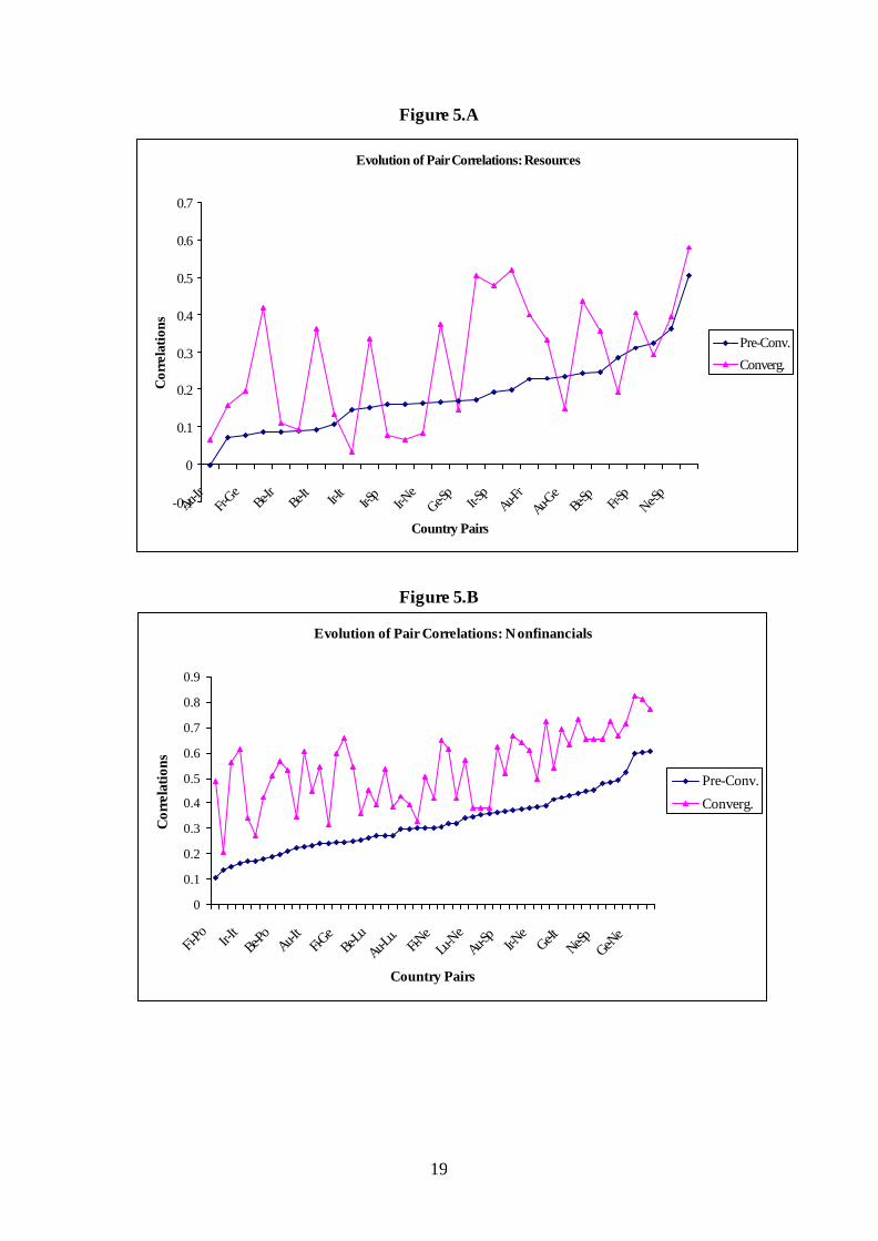
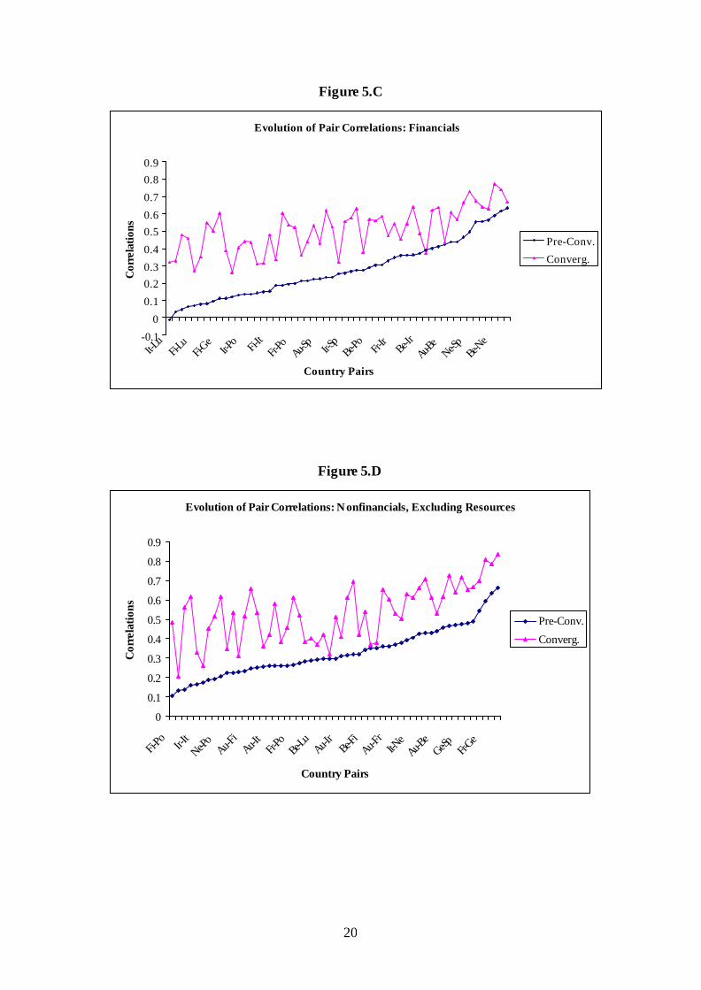
First, consider a broad decomposition into four sectors per country distinguishing the ‘Resources’, ‘Financials’, ’Non-financials’, and ‘Non-financials excluding resources’ (partially overlapping) sectors. Figures 5.A to 5.D report the results when country/sector returns are paired, i.e., we look at the country to country correlations among ‘Financials’ returns, then ‘Non-financials’, etc. Although somewhat less so for the ‘Resources’ sector, the same pattern of increasing correlations over the period under review is observed. Note as well that the sector by sector return correlations tend to be lower than the corresponding correlations using aggregate country indices.

These results are confirmed at a finer level of disaggregation as indicated in Table 9 where a ten-sector decomposition is used. The average (across countries) pair-wise

18

correlations increases in nine sectors out of ten, the UTILS sector being the single exception. The correlation increases range from 4.15 percentage points (from 0.2944 to 0.3359 for the CYSER sector) to 19 points ((from 0.20875 to 0.39883 for the NYCSR sector). Quite understandably, correlation levels are rather lower at this higher level of disaggregation.

19

Figure 5.A

Evolution of Pair Correlations: Resources

-0.1

0

0.1

0.2

0.3

0.4

0.5

0.6

0.7

Au-Ir

Fr-Ge

Be-Ir

Be-It Ir-I

tIr-S

pIr-N

eGe-S

pIt-S

pAu-F

rAu-G

eBe-

Sp Fr-Sp

Ne-Sp

Country Pairs

Cor

rela

tions

Pre-Conv.

Converg.

Figure 5.B

Evolution of Pair Correlations: Nonfinancials

0

0.1

0.2

0.3

0.4

0.5

0.6

0.7

0.8

0.9

Fi-Po Ir-I

tBe-

PoAu-I

tFi-G

eBe-

LuAu-L

u.Fi-N

eLu

-Ne

Au-Sp

Ir-Ne

Ge-ItNe-Sp Ge-N

e

Country Pairs

Cor

rela

tions

Pre-Conv.

Converg.

20

Figure 5.C

Evolution of Pair Correlations: Financials

-0.1

0

0.1

0.20.3

0.4

0.50.6

0.7

0.80.9

It-Lu

Fi-Lu

Fi-Ge

Ir-Po Fi-

ItFr-

PoAu-S

pIr-S

pBe-

Po Fr-Ir

Be-Ir

Au-Be

Ne-Sp

Be-Ne

Country Pairs

Cor

rela

tions

Pre-Conv.

Converg.

Figure 5.D

Evolution of Pair Correlations: Nonfinancials, Excluding Resources

0

0.1

0.2

0.3

0.4

0.5

0.6

0.7

0.8

0.9

Fi-Po Ir-I

tNe-P

oAu-F

iAu-I

tFr-

PoBe-

LuAu-I

rBe-

FiAu-F

rIt-N

eAu-B

eGe-Sp Fr-G

e

Country Pairs

Cor

rela

tions

Pre-Conv.

Converg.

21

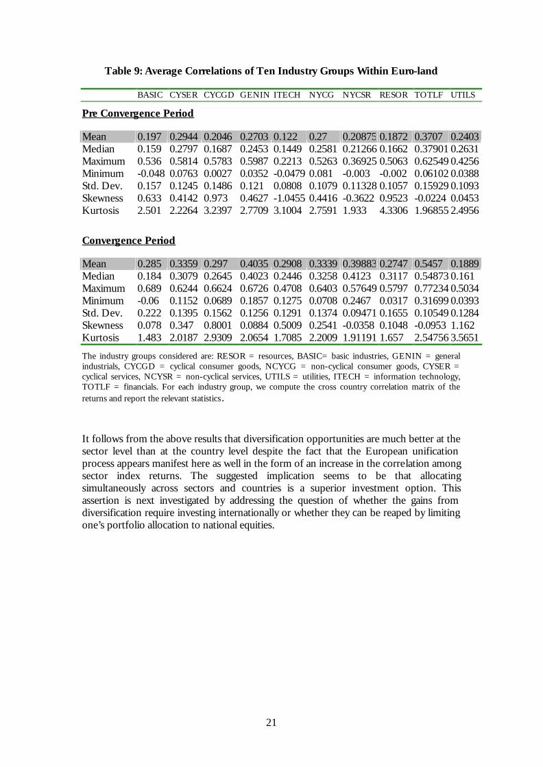
Table 9: Average Correlations of Ten Industry Groups Within Euro-land

BASIC CYSER CYCGD GENIN ITECH NYCG NYCSR RESOR TOTLF UTILS

Pre Convergence Period

Mean 0.197 0.2944 0.2046 0.2703 0.122 0.27 0.20875 0.1872 0.3707 0.2403 Median 0.159 0.2797 0.1687 0.2453 0.1449 0.2581 0.21266 0.1662 0.37901 0.2631 Maximum 0.536 0.5814 0.5783 0.5987 0.2213 0.5263 0.36925 0.5063 0.62549 0.4256 Minimum -0.048 0.0763 0.0027 0.0352 -0.0479 0.081 -0.003 -0.002 0.06102 0.0388 Std. Dev. 0.157 0.1245 0.1486 0.121 0.0808 0.1079 0.11328 0.1057 0.15929 0.1093 Skewness 0.633 0.4142 0.973 0.4627 -1.0455 0.4416 -0.3622 0.9523 -0.0224 0.0453 Kurtosis 2.501 2.2264 3.2397 2.7709 3.1004 2.7591 1.933 4.3306 1.96855 2.4956

Convergence Period

Mean 0.285 0.3359 0.297 0.4035 0.2908 0.3339 0.39883 0.2747 0.5457 0.1889 Median 0.184 0.3079 0.2645 0.4023 0.2446 0.3258 0.4123 0.3117 0.54873 0.161 Maximum 0.689 0.6244 0.6624 0.6726 0.4708 0.6403 0.57649 0.5797 0.77234 0.5034 Minimum -0.06 0.1152 0.0689 0.1857 0.1275 0.0708 0.2467 0.0317 0.31699 0.0393 Std. Dev. 0.222 0.1395 0.1562 0.1256 0.1291 0.1374 0.09471 0.1655 0.10549 0.1284 Skewness 0.078 0.347 0.8001 0.0884 0.5009 0.2541 -0.0358 0.1048 -0.0953 1.162 Kurtosis 1.483 2.0187 2.9309 2.0654 1.7085 2.2009 1.91191 1.657 2.54756 3.5651

The industry groups considered are: RESOR = resources, BASIC= basic industries, GENIN = general industrials, CYCGD = cyclical consumer goods, NCYCG = non-cyclical consumer goods, CYSER = cyclical services, NCYSR = non-cyclical services, UTILS = utilities, ITECH = information technology, TOTLF = financials. For each industry group, we compute the cross country correlation matrix of the returns and report the relevant statistics .

It follows from the above results that diversification opportunities are much better at the sector level than at the country level despite the fact that the European unification process appears manifest here as well in the form of an increase in the correlation among sector index returns. The suggested implication seems to be that allocating simultaneously across sectors and countries is a superior investment option. This assertion is next investigated by addressing the question of whether the gains from diversification require investing internationally or whether they can be reaped by limiting one’s portfolio allocation to national equities.

22

7. The Cost of the Home Bias

The focus here is placed on the characteristics of the optimal portfolios of national investors constrained to investing in home equities and those of optimally diversified portfolios across Euro-land. The diversification in Euro-land can be achieved along two distinct lines: either across countries or across countries and sectors. We use the 10 sector disaggregation of Table 9. Tables 10.A to 10.D report the characteristics of the Minimum Variance Portfolio (MVP) and the Tangent Portfolio (TP) of a European investor selecting freely (without short-selling constraints) among the 10 sector indices either in his home country (French and German perspectives) or in 10 Euro-land countries. Here, we consider the pre-convergence and convergence periods as well. To provide relevant outputs, let Ts ,µ denote the vector of expected returns for a chosen investment opportunity set “s” over a sample period T . “s” refers to country indices when one diversifies by country, to sector indices in the case of an asset allocation by sectors within a given country, or to sector indices when we consider diversification by country and by sector in Euro-land. Ts ,Ω is the variance-covariance matrix associated

with the expected returns of the selected investment opportunity set. If MVPTsW , and

TPTsW , are the vector of weights of the Minimum Variance Portfolio (MVP) and the

Tangent Portfolio (TP) respectively, then:

1'1

11,

1,

, −

−

Ω

Ω=

Ts

TsMVPTsW

TsTs

TsTsTPTsW

,1,

,1,

,'1 µ

µ−

−

Ω

Ω=

Here, 1 is a column vector of ones with the appropriate dimension. Given the portfolio weights TsW , , one can then easily compute the expected return, ( )pRE , and variance,

( )pRV , as well as the Sharpe ratio of the MVP or TP:

( ) TsTsp WRE ,', µ=

( ) TsTsTsp WWRV ,,', Ω=

( )( )p

p

RV

RESharpe =

As is explicit from the computation of the optimal weights of the minimum variance and the tangent portfolios, we abstract from the existence of a riskless asset in our allocation problem. Also, short sales are permitted and the only constraint that we impose is that the portfolio be fully invested (sum of the weights equal to one: 01'1 , =−TsW ). As mentioned above, we provide portfolio characteristics by considering three leading diversification alternatives: 1) diversification by country within Euro-land, 2) diversification by sectors within a given country (France and Germany) and 3) diversification by sectors across Euro-land (focus on countries and sectors simultaneously). For each of these strategies, we provide output for both the pre-convergence and convergence periods.

While our results have to be taken with a grain of salt because no short selling restriction is imposed (with the result that in some instances, the considered portfolios would have

23

included unusually large short positions) 5, the results of the strategy consisting of diversifying by sectors across all of Euro-land are impressively superior (both in terms of the Sharpe ratios and risk of the MVP). Such a strategy would also have permitted a minimal loss of performance between the pre-convergence and the convergence periods despite the increase in correlation of returns noted above.

The home bias – leading to a strategy of diversifying ‘at home’ across industry would have been very costly in terms of both measures of performance, but so is the pure country allocation strategy across Euro-land. On the other hand, limiting one’s investment horizon to the home country would have entailed a minimal loss of performance for either the French or the German investors (the two types of investors considered) if the alternative is a pure country allocation strategy. To put it differently, if the international investment alternative is based on a pure country allocation, the ‘home bias’ is not very costly in terms of performance (Sharpe ratio) or in terms of risk (for the investor interested in the minimum variance portfolio). In fact, for the French investor, a ‘home biased’ portfolio would have outperformed the international ‘country allocation’ strategy during the ‘pre-convergence’ period.

These results underline the sub-optimality of the traditional two-step allocation procedures consisting in first allocating to countries, and then, operating a ‘value oriented’ stock selection within each country. They also suggest that this frequent practice of the investment advisory industry may have a causal relationship with the home bias.

The arguments made above on the cost of the home bias and its implication for optimal portfolio allocation are further reinforced by restricting the analysis to the Consensus Economics sub-periods and using the DMK and FRF as numeraire currencies. As the results in Table 10.E indicate, the convergence period performance ratios are lower, irrespective of the type of portfolio and the currency of reference. Again, the valid alternative portfolio allocation strategy in the post-convergence era seems to be the one focusing on sectors and countries simultaneously.

5 Imposing short selling constraints would amount to using a restricted set of country or sector portfolios. Given the nature of our exercise (which is not meant to identify realistic portfolios), we think it is more informative to preserve the full breadth of our sample of stock returns.

24

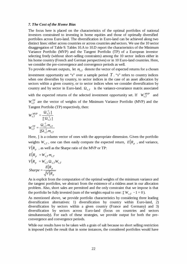
Table 10.A: International Diversification by Country

MVP1 MVP2 TP1 TP2 Austria -0.06933255 0.570661882 -0.62271807 -1.16619701 Belgium 0.308530748 0.470652149 -0.12049101 1.236503643 Finland -0.00208894 -0.11074957 0.192321883 0.318590949 France -0.08367694 -0.03404844 -0.11085488 0.154834482 Germa. 0.068656228 0.083483691 0.143535964 -0.92480574 Ireland -0.0321054 0.256168385 0.281323804 0.939672073 Italy -0.01034946 -0.01726868 -0.2063736 -0.25492938 Netherl. 0.65309373 -0.27128428 1.463967615 0.327838054 Portugal 0.260021694 0.119516657 -0.00957495 -0.01655405 Spain -0.09274911 -0.06713179 -0.01113675 0.385046983 E(Rp) 0.0663 0.10435 0.20462 0.545432 V(Rp) 0.408247 0.738017 1.259972 3.857566 Sharpe 0.103765272 0.12146727 0.18229201 0.277705148

This table gives the weights of country indices in the Minimum Variance Portfolio (MVP) and the Tangent Portfolio (TP). MVP1 and MVP2 stand for pre convergence and convergence Minimum Variance Portfolios respectively, while TP1 and TP2 are the corresponding Tangent Portfolios.

Table 10.B: Diversification by Industry: German Case MVP1 MVP2 TP1 TP2 Basic 0.037579682 0.062220805 0.528788734 0.045000088 Cyclical CG -0.03401575 -0.0075316 -0.72729458 0.120363192 Cyclical Serv. 0.028285357 0.024787093 -0.12361212 0.095861844 General Ind. -0.00740825 -0.08798103 -0.18703055 -0.29005986 Inform. Tech -0.00647038 -0.0289989 0.371687999 0.071076729 Non-cyclical CG -0.06471365 0.01297134 0.168466113 0.189494875 Non-cyclical serv. 0.21049095 0.255489085 0.396243799 0.177823157 Resources 0.097105103 0.070845689 -0.36753543 -0.27940601 Financials -0.01234226 -0.05028437 -0.1778627 -0.042295 Utilities 0.751489187 0.748481884 1.11814874 0.912140978 E(Rp) 0.054796823 0.099563835 0.233041347 0.244106326 V(Rp) 0.370899277 0.394250433 1.577370059 0.966606252 Sharpe 0.089976146 0.158567992 0.185552233 0.248287145

This table gives the weights of German sector indices in the Minimum Variance Portfolio (MVP) and the Tangent Portfolio (TP) in an allocation by sector within Germany. MVP1 and MVP2 stand for pre convergence and convergence Minimum Variance Portfolios respectively, while TP1 and TP2 are the corresponding Tangent Portfolios.

25

Table 10.C: Diversification by Industry: the French Case

MVP1 MVP2 TP1 TP2 Basic 0.36208588 0.332294768 0.259203949 0.183930167 Cyclical CG 0.0543102 -0.22635855 0.710216008 -0.44067269 Cyclical Serv. 0.112585812 0.605366994 -1.08417612 0.700872994 General Ind. -0.08256922 -0.16604577 -0.38574462 -0.11781442 Non-cyclic. CG

0.170272377 0.114348042 1.006522077 0.475409974

Non-cycli. Serv.

0.202783421 0.078369438 0.48664666 0.011633146

Resources 0.118992511 0.12393848 -0.03512431 0.176207984 Financials -0.0368079 0.01797704 -0.53585876 -0.02223691 Utilities 0.098346925 0.120109556 0.578315111 0.032669748 E(Rp) 0.108841419 0.189244698 0.434585734 0.286764745 V(Rp) 0.744838624 0.711841471 2.974017101 1.07866186 Sharpe 0.126113942 0.224301448 0.252001853 0.276110611

This table gives the weights of French sector indices in the Minimum Variance Portfolio (MVP) and the Tangent Portfolio (TP) in an allocation by sector within France. MVP1 and MVP2 stand for pre convergence and convergence Minimum Variance Portfolios respectively, while TP1 and TP2 are the corresponding Tangent Portfolios.

Table 10.D: Euro-land Wide Diversification by Sectors

MVP1 MVP2 TP1 TP2 E(Rp) 0.072706294 0.070393514 0.892045234 0.967017345 V(Rp) 0.104725897 0.115190696 1.284898912 1.58241002 Sharpe 0.224669937 0.207407255 0.786959526 0.768731632

This table gives the weights of sector indices in the Minimum Variance Portfolio (MVP) and the Tangent Portfolio (TP) in an allocation by country and sector. MVP1 and MVP2 stand for pre convergence and convergence Minimum Variance Portfolios respectively, while TP1 and TP2 are the corresponding Tangent Portfolios. The industry groups considered in each Euro-land country are : RESOR = resources (8 indices), BASIC= basic industries(10 indices), GENIN = general industrials(10 indices), CYCGD = cyclical consumer goods(7 indices), NCYCG = non-cyclical consumer goods(10 indices), CYSER = cyclical services(10 indices), NCYSR = non-cyclical services(8 indices), UTILS = utilities(6 indices), ITECH = information technology(5 indices), TOTLF = financials(10 indices). In principle, if each industry group is available in each of the participating countries, then we should have a total of 11 x 10 = 110 investable indices. However, some sectors are not available in some countries so that the number of investable indices is reduced to 84.

26

Table 10.E: Consensus Economics Optimal Portfolio Weights PANEL A: Returns in DMK

MVP1 MVP2 TP1 TP2 Aust 0.3717 NA -0.124 NA Belg 0.1764 0.66452 0.1876 2.15722217 Germ 0.31076 0.01197 0.1594 -1.947099 Spai 0.03135 -0.0725 0.0873 0.42383197 Finl -0.03522 -0.215 -0.0309 1.03349291 Fran 0.00514 0.65668 -0.1584 1.11786848 Irel 0.2526 0.43514 0.5102 0.45547633 Ital -0.04078 -0.073 -0.0466 0.23830925 Neth -0.27758 -0.4987 0.1122 -2.6569123 Port 0.20563 0.09096 0.3032 0.17781023

E(Rp) 0.28975 0.2343 0.436 1.0926901 V(Rp) 0.34502 1.89031 0.5192 8.81558653 Sharpe 0.4933 0.17042 0.6051 0.36801998 PANEL B: Returns in FRF

MVP1 MVP2 TP1 TP2 Aust 0.35174 NA -0.1892 NA Belg 0.1632 0.60309 0.1754 2.01706698 Germ 0.22646 -0.0321 0.0613 -2.7362388 Spai 0.0526 -0.0433 0.1137 0.52227575 Finl -0.06069 -0.2099 -0.056 1.17994922 Fran 0.07425 0.70293 -0.1042 1.87293984 Irel 0.27259 0.4618 0.5537 0.49829915 Ital -0.02441 -0.1154 -0.0308 0.02642717 Neth -0.23966 -0.4583 0.1857 -2.5982244 Port 0.18391 0.09117 0.2904 0.2175051

E(Rp) 0.28088 0.23245 0.4405 1.2162967 V(Rp) 0.36496 1.93997 0.5724 10.1510126 Sharpe 0.46494 0.16689 0.5823 0.3817551

27

8. What Do Our Results Suggest as to the Impact of EMU on the Underlying Economic Structures?

It is helpful at this stage to conceptualise the environment in which the individual investor operates. Variations in firm profitability as reflected in country-wide stock indices result from the interaction of shocks affecting economies, economic structures themselves and their evolution through time, and macro-economic policies. To see this interaction, one may start by inquiring whether the nature of shocks affecting economic agents is impacted by the economic integration process. Let us think of supply shocks first. It is unlikely that the process of economic and monetary integration would result in an increase in the commonness of supply shocks. It may however affect the structure of national economies in a way that technology disturbances will increasingly show up at the country level. This is the case if economic integration increases the degree of specialisation of national economies. At the limit in a one-sector economy, sectoral shock and economy-wide shocks fully coincide. If, however, EMU is accompanied with a higher degree of diversification in national economic structures, supply shocks become less important at the macroeconomic level in the sense that either they wash out (if the number of sectors is large enough and under the plausible assumption that sectoral shocks are little correlated) or they show up as EU-wide risk factor if all the national EMU economies represent the same portfolio of economic sectors.

Thinking of demand shocks now, it is clear that policy shocks within EMU – be they associated with monetary policy (interest rate shocks, foreign exchange shocks) or fiscal policy - are fully or increasingly common in nature. If one believes in the importance of animal spirits, it can similarly be argued that the impact of EMU, if any, must be to make European consumers and investors more alike and subject to the same sort of psychological factors. Finally, demand shocks associated with foreign demand are bound to get more similar under a common currency, besides being influenced by the same structural factors as those discussed above (more common if economies are getting to be more diversified and thus more alike, less so if specialisation is increasing).

In a sense, the above discussion illustrating the interactions between shocks, policies and structures suggests the possibility of two polar outcomes from the process of economic and monetary integration. In the unfavourable case, European economies are getting more specialised, foreign demand shocks translate more and more into differential country shocks calling for differentiated stabilisation policies (at variance with the constraints of a monetary union). The other polar case is one where economic structures become more diversified, countries represent better diversified and also more homogenous portfolios of sectors and common macroeconomic policies are increasingly appropriate. Our results seem to clearly support the latter interpretation of what has been and is currently happening within Euro-land. They appear to accord with a large portion of the recent macro literature. Fatas (1997), among others, looks at the correlation between employment growth rates and finds that European countries represent increasingly better diversified portfolios of regions. Imbs (1999) also finds that developed, increasingly service related economies are getting more and more alike.

9. Conclusions

The conditions under which portfolio investors diversify across the Euro-area equity markets have changed materially in the 1990s. With an increased degree of correlation between either market or sectoral stock indices, diversification opportunities have been

28

significantly reduced. It seems difficult not to incriminate the process of economic and monetary integration process at work in Europe during this period for this result. Within this process, the disappearance of currency risk is decidedly less important for investors than the convergence of economic structures and/or the homogenisation of economic shocks (across the Euro-15 member states). That is, the increased stock return correlations are as manifest when we abstract from currency fluctuations than when they are computed using effective monetary returns. This evolution should mark the end of pure country allocation strategies within Europe. Indeed, if these are the alternatives, the increased conformity of stock returns implies that the cost of the home bias within Euroland has been lowered (in some cases to zero). Diversification across both countries and sectors, however, remains the much superior investment strategy. In light of this option, the cost of the home bias continues to be significant.

29

APPENDIX

Table A: Unconditional Pre and Convergence Periods Summary Statistics

PANEL A: Pre Convergence Summary Statistics

AUSTR BELG. FINL FRAN. GERM IRELA ITALY LUXEM

NETHE

PORTU

SPAIN

Mean -0.0401 0.0319 0.1191 0.0557 0.0301 0.10346 0.006 0.2121 0.0924 0.0161 0.05 Median -0.0705 0.0724 -0.008 0.1291 0.0554 -0.0749 -0.104 0.1084 0.0991 0 -0.0175 Maximum 5.5086 2.5657 6.7605 4.457 4.9172 5.39144 5.084 3.3797 2.3794 2.8432 4.7624 Minimum -7.2925 -3.4116 -6.46 -4.177 -4.5389 -4.4701 -4.879 -1.957 -2.039 -5.291 -4.5158 Std. Dev. 1.3618 0.8583 1.8083 1.19 1.0778 1.30524 1.734 0.8985 0.7593 1.0455 1.4388 Skewness -0.2504 -0.1002 0.4039 0.0657 -0.1896 0.55686 0.149 0.7486 0.067 -0.431 -0.0371 Kurtosis 7.648 4.0832 4.1495 3.864 6.1948 4.93809 3.1 4.1553 2.9708 5.8544 4.0929 Jarque-Bera 204.89 11.377 18.506 7.1605 97.038 46.8431 0.926 23.097 0.1763 83.352 11.248 Probability 0 0.0034 1E-04 0.0279 0 0 0.629 1E-05 0.9156 0 0.0036 Observation 225 225 225 225 225 225 225 155 225 225 225

PANEL B: Convergence Period Summary Statistics Mean 0.0448 0.2183 0.3246 0.192 0.1766 0.25467 0.203 0.1783 0.2323 0.1842 0.2523 Median 0.1237 0.3023 0.3181 0.2492 0.2368 0.26826 0.145 0.2323 0.2456 0.1149 0.3044 Maximum 3.4464 3.8328 5.8755 3.9867 2.7848 3.93614 5.169 6.3828 3.656 5.0664 6.3164 Minimum -3.6196 -5.6564 -8.184 -5.53 -6.5061 -5.9338 -7.438 -5.244 -7.109 -6.502 -5.6296 Std. Dev. 1.0295 1.1174 1.9772 1.3583 1.2891 1.27147 1.801 0.9551 1.395 1.3797 1.5688 Skewness -0.3505 -0.657 -0.994 -0.696 -1.0512 -0.9153 -0.426 0.2961 -1.007 -0.312 -0.3442 Kurtosis 4.3426 6.7352 6.4728 4.9877 6.4779 8.06502 4.802 14.553 8.0789 6.762 5.2008 Jarque-Bera 21.505 146.98 150.15 55.225 154.83 271.93 37.23 1254.5 279.89 136.33 49.852 Probability 2E-05 0 0 0 0 0 0 0 0 0 0 Observation 225 225 225 225 225 225 225 225 225 225 225 This table gives the unconditional summary statistics of the first sub-sample (pre convergence period) of the Euro-land index returns (in Euro). The sub-sample runs from September 10, 1990 to December 26, 1994 and observations are sampled weekly. Returns are continuously compounded and annualized.

30

Table B: Pre and Convergence Period Correlation Matrices

PANEL A: Pre Convergence Correlation Matrix

Austria 1 Belgium 0.493 1 Finland 0.252 0.342 1 France 0.400 0.424 0.3323 1 Germany 0.499 0.491 0.2569 0.6219 1 Ireland 0.357 0.44 0.2601 0.3603 0.324 1 Italy 0.218 0.213 0.2456 0.3543 0.4228 0.1539 1 Luxemb. 0.287 0.307 0.1361 0.1731 0.3087 0.3196 0.0593 1 Netherl. 0.499 0.562 0.3291 0.6522 0.6305 0.4895 0.4102 0.332 1 Portugal 0.171 0.257 0.0763 0.2643 0.2414 0.2451 0.1052 0.091 0.2254 1 Spain 0.371 0.413 0.2237 0.5388 0.5076 0.2975 0.3692 0.178 0.5388 0.271 1

PANEL B: Convergence Period Correlation Matrix

Austria 1 Belgium 0.577 1 Finland 0.542 0.591 1 France 0.635 0.745 0.6308 1 Germany 0.632 0.759 0.6835 0.8069 1 Ireland 0.483 0.509 0.5417 0.5271 0.6162 1 Italy 0.479 0.631 0.5551 0.6886 0.6397 0.437 1 Luxemb. 0.445 0.438 0.3303 0.4218 0.4388 0.3863 0.3604 1 Netherl. 0.666 0.784 0.6819 0.7931 0.8512 0.602 0.6481 0.497 1 Portugal 0.47 0.624 0.4961 0.6249 0.6375 0.4864 0.5504 0.337 0.6316 1 Spain 0.561 0.683 0.5946 0.7097 0.7569 0.5356 0.7006 0.368 0.75 0.616 1

This table gives the unconditional correlations of the pre and convergence periods of the Euro-land index returns (in Euro).

31

Table C : Unconditional Correlations of Other Regions of the World

PANEL A: Pre Convergence Correlations

AMERICAS 1 ASIA 0.1676907 1 AUSTRALASIA 0.3420364 0.304517 1 EEC 0.4502127 0.489253 0.3411 1 FAR_EAST01 0.1626266 0.9985 0.295 0.47406 1 NON_EEC01 0.3653845 0.378988 0.2942 0.73584 0.36538 1 PACIFIC_BASIN01 0.1784735 0.999236 0.3265 0.49204 0.99842 0.38137 1 PANEL B: Convergence Period Correlations AMERICAS 1 ASIA 0.340735 1 AUSTRALASIA 0.53693 0.581872 1 EEC 0.609744 0.520372 0.5587 1 FAR_EAST01 0.314605 0.992436 0.5446 0.49291 1 NON_EEC01 0.48334 0.510832 0.4704 0.84359 0.48922 1 PACIFIC_BASIN01 0.358277 0.998625 0.6164 0.53208 0.99059 0.51753 1

32

Table D: Unconditional Correlations (Returns in DMK) PANEL A: Pre Convergence Period

Aust 1 Belg 0.53660 1 Germ 0.42548 0.61400 1 Spai 0.34662 0.53700 0.51013 1 Finl 0.22558 0.43324 0.32515 0.44608 1 Fran 0.44165 0.64169 0.64824 0.58506 0.44458 1 Irel 0.56784 0.56479 0.39787 0.32783 0.47566 0.5190 1 Ital 0.13218 0.27485 0.48755 0.39328 0.32058 0.3401 0.1178 1 Luxe 0.51173 0.44318 0.15807 0.08708 0.21185 0.2583 0.4833 -0.131 1 Neth 0.55339 0.66233 0.68473 0.60430 0.53363 0.6626 0.6735 0.38571 0.3956 1 Port 0.32355 0.32783 0.27588 0.36832 0.36315 0.3865 0.3571 0.35229 0.0611 0.3088 1 PANEL B: Convergence Period

Aust 1 Belg 0.54415 1 Germ 0.61771 0.76077 1 Spai 0.53261 0.67593 0.75791 1 Finl 0.57565 0.58523 0.71716 0.62506 1 Fran 0.59345 0.71413 0.79854 0.71750 0.63393 1 Irel 0.54165 0.50692 0.61905 0.55238 0.58875 0.5897 1 Ital 0.40944 0.58876 0.61559 0.68786 0.55865 0.6715 0.4939 1 Luxe 0.45167 0.49397 0.47167 0.42956 0.38286 0.4831 0.4794 0.38157 1 Neth 0.65913 0.76101 0.84972 0.73301 0.71369 0.7806 0.664 0.59127 0.5045 1 Port 0.50001 0.63002 0.68002 0.64024 0.51435 0.6612 0.4643 0.55410 0.4351 0.6640 1

33

Table E: Unconditional Correlations (Returns in FRF) PANEL A: Pre Convergence Period

Aust 1 Belg 0.544759 1 Germ 0.447629 0.6481 1 Spai 0.320727 0.50972 0.49896 1 Finl 0.212673 0.42360 0.32802 0.43437 1 Fran 0.407621 0.61340 0.64224 0.56586 0.43029 1 Irel 0.571723 0.57090 0.41642 0.31698 0.47287 0.5115 1 Ital 0.111494 0.25914 0.47427 0.37989 0.31048 0.3208 0.1090 1 Luxe 0.505567 0.46604 0.19873 0.05718 0.20135 0.2179 0.4893 -0.1525 1 Neth 0.545713 0.66567 0.69838 0.58657 0.52613 0.6417 0.6774 0.37051 0.3907 1 Port 0.315576 0.33706 0.29318 0.35213 0.35614 0.3651 0.3590 0.34090 0.0560 0.3023 1 PANEL B: Convergence Period

Aust 1 Belg 0.560095 1 Germ 0.624814 0.76615 1 Spai 0.515230 0.66354 0.74898 1 Finl 0.562725 0.57482 0.70905 0.61659 1 Fran 0.565067 0.69744 0.78857 0.70390 0.62503 1 Irel 0.511510 0.48560 0.60279 0.52877 0.57751 0.5547 1 Ital 0.379878 0.56544 0.59664 0.67469 0.54617 0.6549 0.4662 1 Luxe 0.453979 0.50558 0.47534 0.40233 0.36547 0.4356 0.4314 0.34241 1 Neth 0.649089 0.75488 0.84613 0.72360 0.70777 0.7693 0.6459 0.57307 0.4860 1 Port 0.507949 0.63725 0.68413 0.63195 0.50716 0.6499 0.4457 0.53693 0.4382 0.6603 1

34

Table F: Currency Returns PANEL A: DMK Returns Against Other Euro-land Currencies ATS BEF ESP FMK FRF IRP ITL LUF NLG PSC Mean 0.002639 0.0008 -0.03305 -0.02625 0.003885 -0.007 -0.0339 0.00262 0.00303 -0.0169 Median 0.005454 0.003028 -0.00514 -0.00397 0.016873 0.02536 -0.0074 0.00457 0.00464 -0.0017 Maximum 1.887337 1.962902 1.64792 2.13159 1.391829 1.84225 2.6263 0.89609 1.74339 1.5577 Minimum -1.79991 -1.65267 -4.13025 -5.91884 -1.44092 -4.9629 -5.07 -0.84166 -1.5620 -2.644 Std. Dev. 0.365714 0.345744 0.49111 0.64257 0.349599 0.57194 0.5989 0.21593 0.39249 0.3575 Skewness -0.11509 0.369364 -1.72232 -2.85751 -0.24802 -1.7080 -1.9056 -0.03205 0.00547 -1.8214 Kurtosis 7.240137 11.99241 15.6363 26.8432 5.326523 16.5303 18.905 5.36255 6.57419 16.069 J-Bera 314.0529 1417.876 2987.71 10470.2 98.55711 3391.69 4659.0 60.5124 222.497 3206.0 Probability 0 0 0 0 0 0 0 0 0 0 Observ. 418 418 418 418 418 418 418 260 418 418

PANEL B: FRF Returns Against Other Euro-land Currencies Mean -0.001247 -0.00308 -0.00389 -0.03694 -0.03013 -0.0108 -0.0378 -0.00065 -0.0008 -0.0208 Median -0.012703 -0.01966 -0.01687 -0.03089 -0.00504 -0.0012 -0.0209 -0.00804 -0.0112 -0.0114 Maximum 2.146706 1.661731 1.44092 1.41996 1.581367 1.65214 2.0754 1.22244 2.00276 1.7372 Minimum -1.497532 -1.60836 -1.39183 -4.39867 -5.70711 -4.5014 -3.6291 -1.13835 -1.5483 -2.4522 Std. Dev. 0.353941 0.400917 0.34959 0.41529 0.577941 0.49808 0.5685 0.24317 0.34025 0.4203 Skewness 0.472881 0.270928 0.24802 -3.05414 -3.31913 -1.7410 -0.991 0.1087 0.62903 -0.7327 Kurtosis 9.207642 6.207924 5.32652 34.0739 33.20284 19.1469 9.7371 8.80195 9.61644 7.5216 J-Bera 686.7267 184.3447 98.55711 17467.18 16655.18 4752.06 858.944 365.1914 790.02 393.487 Probability 0 0 0 0 0 0 0 0 0 0 Observ 418 418 418 418 418 418 418 260 418 418

35

Table G: Optimal Portfolio Characteristics: Returns in DMK MVP1 MVP2 TP1 TP2

Aust -0.0584431 0.60325417 -0.8616618 -1.6385557 Belg 0.35738194 0.44686837 0.16754626 1.73530373 Germ 0.22755863 0.19483068 0.59428564 -0.9214717 Spai -0.0673971 -0.0657429 -0.3193248 0.46474210 Finl -0.0049129 -0.1361071 0.17908531 0.33532885 Fran -0.0679396 -0.0141340 -0.078210 -0.1561431 Irel -0.0664060 0.19495807 0.12538742 1.06092540 Ital -0.0077568 -0.0287811 -0.2268347 -0.3998143

Neth 0.41922977 -0.3195902 1.45244209 0.05966042 Port 0.26868537 0.12444432 -0.0327146 0.46002446

E(Rp) 0.08325919 0.09223738 0.26998220 0.71701031 V(Rp) 0.50956860 0.75236939 1.65236348 5.84856791 Sharpe 0.11663553 0.10633871 0.21003048 0.29648357

Table H: Optimal Portfolio Characteristics: Returns in FRF MVP1 MVP2 TP1 TP2

Aust -0.0363346 0.56595838 -0.8263275 -1.7340071 Belg 0.30999706 0.37715379 0.12328722 1.69901289 Germ 0.04836573 0.08039663 0.40905420 -1.0648642 Spai -0.0490738 -0.0408689 -0.2968532 0.503377 Finl 0.00105510 -0.1376628 0.182023682 0.34600287 Fran 0.09422818 0.10784828 0.08412622 -0.0378447 Irel -0.0834778 0.25357643 0.10515755 1.14200811 Ital -0.0200508 -0.0216542 -0.2355214 -0.4023124 Neth 0.49427053 -0.2841058 1.51046993 0.10498313 Port 0.24102058 0.09935833 -0.0554165 0.44364387 E(Rp) 0.08942705 0.09472654 0.27307546 0.73570692 V(Rp) 0.53830537 0.79271737 1.64377547 6.15674983 Sharpe 0.12188620 0.10639287 0.21299109 0.29650299

36

REFERENCES

Adler, M. and B. Dumas, (1983), ‘International portfolio choice and corporate finance: a synthesis’, Journal of Finance, June

Ammer, J. and J. Mei, (1996), ‘Measuring international economic linkages with stock market data’, Journal of Finance, 51, 1743-1763

Barr, D. and R. Priestley, (1998), ‘Expected returns, risk and the integration of international bond markets’, Norwegian School of Management

Bekaert, G. and C. Harvey, (1995), ‘Time-varying world market integration’, Journal of Finance 50, 403-444

Canova, F. and J. Marrinan, (1998), ‘Sources and propagation of international output cycles: common shocks or transmission?’, Journal of International Economics 46, 133-166

Cooper, I. and C. Kaplanis, (1986), ‘Costs to crossborder investment and international equity market equilibrium’, In: J. Edwards et al., eds., Recent Advances in Corporate Finance (Cambridge University Press)

Dermine, J. and P. Hillion, (1999) (eds), ‘European Capital Markets with a Single Currency’, Oxford University Press

De Santis, G., B. Gerard, and P. Hillion, (1998), ‘International portfolio management, currency risk and the Euro’, Unpublished Draft

De Santis, G., B. Gerard, and P. Hillion, (1999), ‘The single European currency and world equity markets’, in European Capital Markets with a Single Currency, Oxford University Press

Easley, D. and M. O'Hara, (1992), ‘Time and the process of security price adjustment‘, Journal of Finance, 47/2, 577-605

Fatas, A, (1997), ‘EMU: Countries or regions?’ European Economic Review 41

Ferson, W. and C. Harvey, (1991), ‘The variation of economic risk premiums’, Journal of Political Economy 99, 285-315

Forni, M. and L. Reichlin, (1997), ‘National policies and local economies: Europe and the United States’, CEPR Discussion Paper 1632

French and Poterba, (1991), ‘Investor diversification and the equity markets’, American Economic Review

Golub, S.S. (1990), ‘International capital mobility: Net versus gross stocks and flows’, Journal of International Money and Finance, 9, 424-439.

Hansen, L. (1982), ‘Large sample properties of generalized method of moments estimators‘, Econometrica , vol. 50/4, 1029-1054.

Hardouvelis, G., D. Malliaropolous and R. Priestly, (1999) ‘EMU and European Stock Market Integration’,' CEPR Discussion Paper No. 2124.

Harvey, C. (1991), ‘The world price of covariance risk’, Journal of Finance 46, 111-157

Heston, S. and G. Rouwenhorst, (1994), ‘Does industrial structure explain the benefits of international diversification?’ Journal of Financial Economics 36, 3-27

37

Heston, S. and G. Rouwenhorst, (1995), ‘Industry and country effects in international stock returns’, Journal of Portfolio Management 21, 53-58

Imbs, J. (1998), ‘Co-Fluctuations’, DEEP Working Paper 9819, Université de Lausanne

Jenrich, J. (1970), ‘An asymptotic chi-square test for the equality of two correlation matrices’, Journal of the American Statistical Association 65, 904-912

Kaplanis, E. (1988), ‘Stability and forecasting of co-movement measures of international stock market return’, Journal of International Money and Finance 8, 63-75

Lamedica, P. (1999), Euro Asset Allocation, Paribas, London. Lewis, K. (1995), ‘Puzzles in International Financial Markets’, in Handbook of International Economics. Gene Grossmann and Kenneth Rogoff, eds Amsterdam: North Holland, pp. 1913-71 Lewis, K. (1999), ‘Trying to explain Home Bias in Equities and Consumption’, Journal of Economic Literature, vol. 38 (june 1999), 571-608 Longin, F. and B. Solnik, (1995), ‘Is the correlation in international equity returns constant: 1960-1990?’, Journal of International Money and Finance 41(1), 3-26

Obstfeld, M. (1994), ‘Risk-taking Global Diversification and Growth’, American Economic Review, 84:5, 1471-86 Restoy, F. and R. Rodriguez, (1998), ‘Can fundamentals explain cross-country correlations of asset returns?’, CEPR Discussion Paper 1996

Rouwenhorst G. (1998), ‘European equity markets and EMU: are the differences between countries slowly disappearing?’, Unpublished Draft, Yale University

Tesar, L.L. and I. Werner, ‘Home bias and the globalization of securities’, NBER WP n.4218

Tesar, L.L. and I.Werner (1994), ‘International equity transaction and the US portfolio choice’, In :J. A. Frankel, ed., The internalization of equity markets (University of Chicago press)

Tesar, L. and I. Werner (1995), ‘Home bias and high turnover’, Journal of International Money and Finance, 14(2), 467-492

RESEARCH PAPER SERIES

Extra copies of research papers will be available to the public upon request. In order to obtain copies of past or future works, please contact our office at the location below. As well, please note that these works will be available on our website, www.fame.ch, under the heading "Research" in PDF format for your consultation. We thank you for your continuing support and interest in FAME and look forward to serving you in the future.

N. 30: Serial and Parallel Krylov Methods for Implicit Finite Difference Schemes Arising in Multivariate Option

Pricing Manfred GILLI, University of Geneva, Evis KËLLEZI, University of Geneva and FAME, Giorgio PAULETTO, University of Geneva, March 2001

N. 29: Liquidation Risk Alexandre ZIEGLER, HEC-University of Lausanne, Darrell DUFFIE, The Graduate School of Business, Stanford University; April 2001

No 28: Defaultable Security Valuation and Model Risk Aydin AKGUN, University of Lausanne and FAME; March 2001

No 27: On Swiss Timing and Selectivity: in the Quest of Alpha François-Serge LHABITANT, HEC-University of Lausanne and Thunderbird, The American Graduate School of International Management; March 2001

No 26: Hedging Housing Risk Peter ENGLUND, Stockholm School of Economics, Min HWANG and John M. QUIGLEY, University of California, Berkeley; December 2000

N° 25: An Incentive Problem in the Dynamic Theory of Banking Ernst-Ludwig VON THADDEN, DEEP, University of Lausanne and CEPR; December 2000

N° 24: Assessing Market Risk for Hedge Funds and Hedge Funds Portfolios François-Serge LHABITANT, Union Bancaire Privée and Thunderbird, the American Graduate School of International Management; March 2001

N° 23: On the Informational Content of Changing Risk for Dynamic Asset Allocation Giovanni BARONE-ADESI, Patrick GAGLIARDINI and Fabio TROJANI, Università della Svizzera Italiana; March 2000

N° 22: The Long-run Performance of Seasoned Equity Offerings with Rights: Evidence From the Swiss Market Michel DUBOIS and Pierre JEANNERET, University of Neuchatel; January 2000

N° 21: Optimal International Diversification: Theory and Practice from a Swiss Investor's Perspective Foort HAMELINK, Tilburg University and Lombard Odier & Cie; December 2000

N° 20: A Heuristic Approach to Portfolio Optimization Evis KËLLEZI; University of Geneva and FAME, Manfred GILLI, University of Geneva, October 2000

N° 19: Banking, Commerce, and Antitrust Stefan Arping; University of Lausanne; August 2000

N° 18: Extreme Value Theory for Tail-Related Risk Measures Evis KËLLEZI; University of Geneva and FAME, Manfred GILLI, University of Geneva; October 2000

N° 17: International CAPM with Regime Switching GARCH Parameters Lorenzo CAPIELLO, The Graduate Institute of International Studies; Tom A. FEARNLEY, The Graduate Institute of International Studies and FAME; July 2000

INTERNATIONAL CENTER FOR FINANCIAL ASSET MANAGEMENT AND ENGINEERING 40 bd du Pont d'Arve • P.O. Box 3 • CH-1211 Geneva 4 • tel +41 22 / 312 0961 • fax +41 22 / 312 1026

http://www.fame.ch • e-mail: admin@fame.ch

N° 16: Prospect Theory and Asset Prices Nicholas BARBERIS, University of Chicago; Ming HUANG, Stanford University; Tano SANTOS, University of Chicago; September 2000

N° 15: Evolution of Market Uncertainty around Earnings Announcements Dušan ISAKOV, University of Geneva and FAME; Christophe PÉRIGNON, HEC-University of Geneva and FAME; June 2000

N° 14: Credit Spread Specification and the Pricing of Spread Options Nicolas MOUGEOT, IBFM-University of Lausanne and FAME, May 2000

N° 13: European Financial Markets After EMU: A First Assessment Jean-Pierre DANTHINE, Ernst-Ludwig VON THADDEN, DEEP, Université de Lausanne and CEPR and Francesco GIAVAZZI, Università Bocconi, Milan, and CEPR; March 2000

N° 12: Do fixed income securities also show asymmetric effects in conditional second moments? Lorenzo CAPIELLO, The Graduate Institute of International Studies; January 2000

N° 11: Dynamic Consumption and Portfolio Choice with Stochastic Volatility in Incomplete Markets George CHACKO, Harvard University; Luis VICEIRA, Harvard University; September 1999

N° 10: Assessing Asset Pricing Anomalies Michael J. BRENNAN, University of California, Los Angeles; Yihong XIA, University of California, Los Angeles; July 1999

N° 9: Recovery Risk in Stock Returns Aydin AKGUN, University of Lausanne & FAME; Rajna GIBSON, University of Lausanne; July 1999

N° 8: Option pricing and replication with transaction costs and dividends Stylianos PERRAKIS, University of Ottawa; Jean LEFOLL, University of Geneva; July1999

N° 7: Optimal catastrophe insurance with multiple catastrophes Henri LOUBERGÉ, University of Geneva; Harris SCHLESINGER, University of Alabama; September 1999

N° 6: Systematic patterns before and after large price changes: Evidence from high frequency data from the Paris Bourse Foort HAMELINK, Tilburg University; May 1999

N° 5: Who Should Buy Long-Term Bonds? John CAMPBELL, Harvard University; Luis VICEIRA, Harvard Business School; October 1998

N° 4: Capital Asset Pricing Model and Changes in Volatility André Oliveira SANTOS, Graduate Institute of International Studies, Geneva; September 1998

N° 3: Real Options as a Tool in the Decision to Relocate: An Application to the Banking Industry Pascal BOTTERON, HEC-University of Lausanne; January 2000

N° 2: Application of simple technical trading rules to Swiss stock prices: Is it profitable ? Dušan ISAKOV, HEC-Université de Genève; Marc HOLLISTEIN, Banque Cantonale de Genève; January 1999

N° 1:

Enhancing portfolio performance using option strategies: why beating the market is easy. François-Serge LHABITANT, HEC-University of Lausanne; December 1998

International Center FAME - Partner Institutions

The University of Geneva The University of Geneva, originally known as the Academy of Geneva, was founded in 1559 by Jean Calvin and Theodore de Beze. In 1873, The Academy of Geneva became the University of Geneva with the creation of a medical school. The Faculty of Economic and Social Sciences was created in 1915. The university is now composed of seven faculties of science; medicine; arts; law; economic and social sciences; psychology; education, and theology. It also includes a school of translation and interpretation; an institute of architecture; seven interdisciplinary centers and six associated institutes.

More than 13’000 students, the majority being foreigners, are enrolled in the various programs from the licence to high-level doctorates. A staff of more than 2’500 persons (professors, lecturers and assistants) is dedicated to the transmission and advancement of scientific knowledge through teaching as well as fundamental and applied research. The University of Geneva has been able to preserve the ancient European tradition of an academic community located in the heart of the city. This favors not only interaction between students, but also their integration in the population and in their participation of the particularly rich artistic and cultural life. http://www.unige.ch The University of Lausanne Founded as an academy in 1537, the University of Lausanne (UNIL) is a modern institution of higher education and advanced research. Together with the neighboring Federal Polytechnic Institute of Lausanne, it comprises vast facilities and extends its influence beyond the city and the canton into regional, national, and international spheres. Lausanne is a comprehensive university composed of seven Schools and Faculties: religious studies; law; arts; social and political sciences; business; science and medicine. With its 9’000 students, it is a medium-sized institution able to foster contact between students and professors as well as to encourage interdisciplinary work. The five humanities faculties and the science faculty are situated on the shores of Lake Leman in the Dorigny plains, a magnificent area of forest and fields that may have inspired the landscape depicted in Brueghel the Elder's masterpiece, the Harvesters. The institutes and various centers of the School of Medicine are grouped around the hospitals in the center of Lausanne. The Institute of Biochemistry is located in Epalinges, in the northern hills overlooking the city. http://www.unil.ch The Graduate Institute of International Studies The Graduate Institute of International Studies is a teaching and research institution devoted to the study of international relations at the graduate level. It was founded in 1927 by Professor William Rappard to contribute through scholarships to the experience of international co-operation which the establishment of the League of Nations in Geneva represented at that time. The Institute is a self-governing foundation closely connected with, but independent of, the University of Geneva. The Institute attempts to be both international and pluridisciplinary. The subjects in its curriculum, the composition of its teaching staff and the diversity of origin of its student body, confer upon it its international character. Professors teaching at the Institute come from all regions of the world, and the approximately 650 students arrive from some 60 different countries. Its international character is further emphasized by the use of both English and French as working languages. Its pluralistic approach - which draws upon the methods of economics, history, law, and political science -reflects its aim to provide a broad approach and in-depth understanding of international relations in general. http://heiwww.unige.ch