ORIGINAL ARTICLE Open Access

Opportunities for peak shaving the energydemand of ship-to-shore quay cranes atcontainer terminalsHarry Geerlings1*, Robert Heij2ˆ and Ron van Duin2,3

* Correspondence: Geerlings@essb.eur.nlˆDeceased1Erasmus University Rotterdam,Erasmus School of Social andBehavioural Sciences/ ErasmusSmart Port, P.O. box 1738, 3000 DRRotterdam, The NetherlandsFull list of author information isavailable at the end of the article

Abstract

This paper presents the results of both a qualitative and a quantitative study onthe possibilities for peak shaving the energy demand of ship-to-shore (STS) cranesat container terminals. The objective is to present an energy consumption modelthat visualizes the energy demand of STS cranes and to show the possibilities forreducing the peak demand of STS cranes by implementing rules of operation (i.e.changes to the business operational procedures). The results show that the peakdemand (and peak-related costs) can be reduced by 50%, with an increase in thehandling time of containerships of less than half a minute per hour handling time.This can be achieved by reducing the maximum energy demand of all operatingSTS cranes or by limiting the maximum number of simultaneously lifting STScranes. If (one of) these rules of operation is implemented, an intermediate containerterminal with six to eight STS cranes can save up to €250,000 per year, which is about48% of total peak-related energy costs.

Keywords: Peak shaving, Container terminals, Electricity demand, Energy consumption,Ship-to-shore cranes

IntroductionGrowth in containerized transport

The worldwide throughput of containers is growing continuously. The standardized

size of containers (in 20 ft. and 40 ft. equivalent units) makes them a suitable means

for transporting all kinds of products, ranging from multimedia and building mate-

rials to clothing and shoes. Even temperature-sensitive goods like flowers, fruits, and

vegetables can be transported easily by temperature-controlled containers, known as

reefers. The share of containerized transport in seaborne trade increased from 2.75%

in 1980 to 15% in 2014 (UNCTAD 2015.), and total seaborne trade increased to

9842 million tons (UNCTAD 2015). The annual worldwide transport of containers

increased from 28.7 million twenty-foot equivalent units (TEU) in 1990 to 171 mil-

lion TEU in 2014 (UNCTAD 2015) The 20-year average growth percentage of the

container market is a remarkable 7.8% (Clarksons 2015; Port of Rotterdam 2015).

An important development that facilitates the growing container market is the in-

creasing capacities of containerships. Whereas the largest containership in 1980 had

Journal of Shipping and Trade

© The Author(s). 2018 Open Access This article is distributed under the terms of the Creative Commons Attribution 4.0 InternationalLicense (http://creativecommons.org/licenses/by/4.0/), which permits unrestricted use, distribution, and reproduction in any medium,provided you give appropriate credit to the original author(s) and the source, provide a link to the Creative Commons license, andindicate if changes were made.

Geerlings et al. Journal of Shipping and Trade (2018) 3:3 https://doi.org/10.1186/s41072-018-0029-y

a capacity of 3000 TEU, the largest containerships operating in 2015 have a capacity

of almost 20,000 TEU (Lloyd's List 2015).

The growing size of containerships influences container terminal operations, as

the number of containers per containership has also increased as a result of this de-

velopment. Container carriers demand that container terminals handle their ships

as fast as possible to continue their journey to the next port. This higher productiv-

ity is achieved by more automated terminal processes (Grunow et al. 2005) and by

deploying more terminal equipment simultaneously. However, with more and more

simultaneously operating ship-to-shore (STS) cranes, the energy demand (kW/s) in-

creases. This also increases the highest observed peak demand, leading to a higher

energy bill and therefore higher handling costs.

Container terminals’ peak demand is responsible for about 25–30% of the monthly

energy bill (Personal communication, ABB, a worldwide provider of electrotechnical so-

lutions for the shipping, offshore, and harbour industries (ABB 2014; Stedin 2014). The

main reason is that the highest observed peak demand is charged for the next

12 months. To illustrate this: if the highest peak in January is 12,000 kW, the terminal

is charged for 12,000 kW for the rest of the year. However, if the highest peak in March

is 14,000 kW, the terminal is charged for 14,000 kW until March the year after. A

lower peak demand could result in large annual savings for container terminals. It is

consequently very important to investigate the possibilities of reducing this peak

demand.

The research question

The research objective is therefore to investigate the possibilities for peak shaving the

electricity demand at container terminals by applying new rules of operation for

electricity-consuming terminal processes, while also monitoring the consequences for the

handling speed of containerships. Peak shaving implies the lowering of the highest ob-

served peak in energy demand to reduce the energy-related costs. This enables container

terminals to lower the handling costs of containerships, giving them a better competitive

position. Another advantage of peak shaving is that terminals’ energy demand is more

stable; this is especially important for container terminals in countries where grid opera-

tors cannot prepare the energy system for unexpected high energy peaks. The handling

time for containerships needs to be monitored, because extra handling time might affect a

terminal’s competitive position. The main research question addressed in this research is:

What are the possibilities for reducing the peak demand of electricity-consuming terminal

equipment (peak shaving) in order to reduce the electricity-related energy costs? The hy-

pothesis is that, by implementing different rules of operation (i.e. process improvements),

like limiting the number of lifting cranes or the maximum allowed energy, terminals are

able to reduce the height of peaks and thereby reduce their energy-related costs.

This paper presents the results of this research by discussing STS cranes’ ter-

minal operations and the volatility of their energy demand in section 2. Both the

methodology applied and the study’s relevance are presented in this section as

well. Section 3 presents the energy consumption model, which forms the basis for

the simulation model developed. The simulation model is presented in section 4,

and the results of the simulation study are discussed in section 5. Finally, the

Geerlings et al. Journal of Shipping and Trade (2018) 3:3 Page 2 of 20

implications of these results and the conclusions of the study are discussed in sec-

tions 6 and 7.

Research and methodologySTS crane operations

After a containership has berthed at the seaside of a terminal, the STS cranes start

unloading the incoming containers according to the unloading plan. STS cranes can use a

normal spreader, enabling them to handle one container at a time, or more advanced

spreaders (e.g. the twin-lift and tandem-lift) to handle multiple containers at the same

time (Stahlbock and Voß 2008). The Super Post Panamax STS cranes, the current stand-

ard for unloading the largest containerships, are able to make approximately 32 lifts per

crane per hour (APM Terminals 2014). This allows an STS crane to handle 32–64 TEUs

per hour with a normal spreader and up to 128 TEUs per hour with a tandem-lift

spreader.

The handling capacity of a container terminal is highly dependent on the number of

STS cranes and their capacity, as the cranes determine the handling time per ship as

well as the throughput of containers to the stacking process (Eugen et al. 2014).

During the (un)loading of a containership, two criteria are important: the ship’s

stability and the number of unproductive moves (Imai et al. 2006). During (un)load-

ing, the ship’s stability changes as a result of the continuously changing container

load. Because containerships visit several container terminals, each time unloading

containers from and loading containers onto the ship, not all containers that have to

be unloaded are positioned on top of the ship’s stacks. Ships therefore have to be

loaded in an efficient way, allowing the next container terminal to unload the con-

tainership with a minimum of unproductive moves.

These two criteria are often in conflict, because the most efficient loading (regarding

the minimization of unproductive moves) might not be in line with the most efficient

loading regarding the ship’s stability. This makes stowage very complex (Bortfeldt and

Gehring 2001; Steenken et al. 2004; Dekker et al. 2006), especially because the stowage

plans have to be aligned over all the different ports that have to (un)load the ship (Wilson

and Roach 2000).

Volatility of energy demand

The STS cranes are connected to the electricity network. For all quay crane processes

(moving of crane and spreader, crane lighting, and auxiliary processes), electricity is

supplied by the network. Vertical movements have the most volatile energy demand,

showing high peaks for hoisting the crane spreader and low falls for lowering the

spreader, as can be seen in Fig. 1 (MSC Terminal Valencia 2009, field data). The gantry

(horizontal) movements and auxiliary energy consumption are less volatile in character.

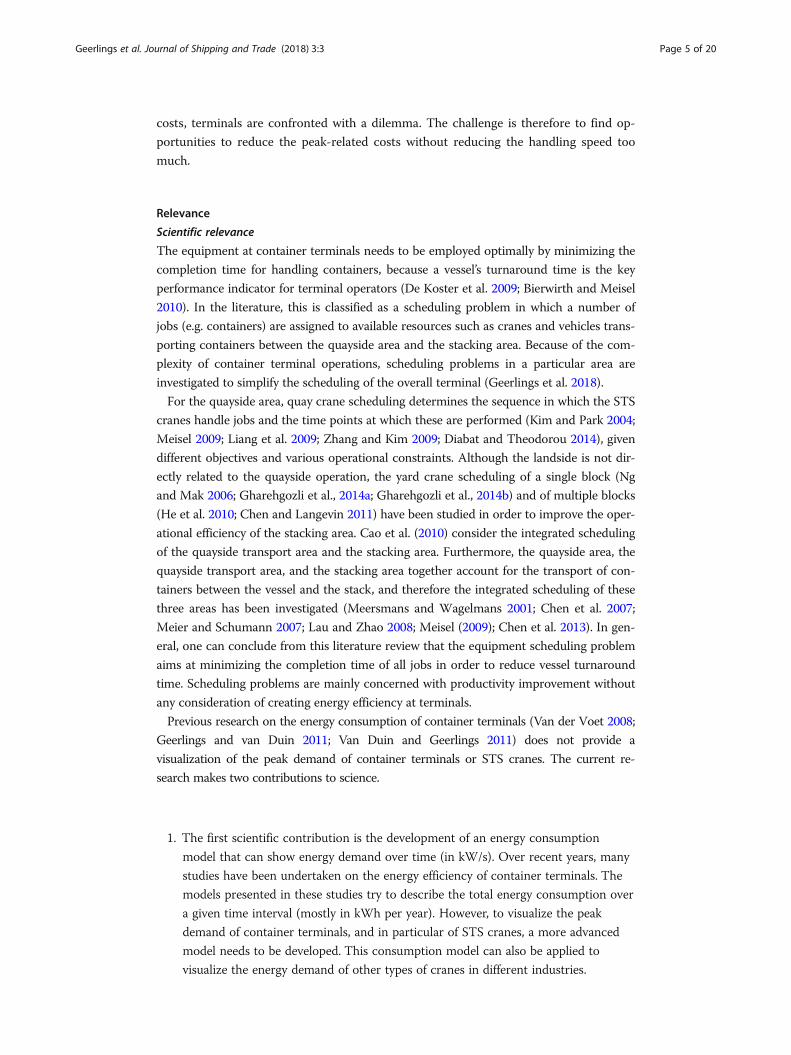
In Fig. 2, the total energy consumption for one STS crane is visualized. In total, two

peaks can be identified for handling a container: the first for lifting a spreader and con-

tainer above the ship and the second for lifting the spreader after the container is posi-

tioned in the terminal. When all STS cranes in a terminal are lifting at the same

moment, the potential peak demand is very high. It is therefore important to visualize

Geerlings et al. Journal of Shipping and Trade (2018) 3:3 Page 3 of 20

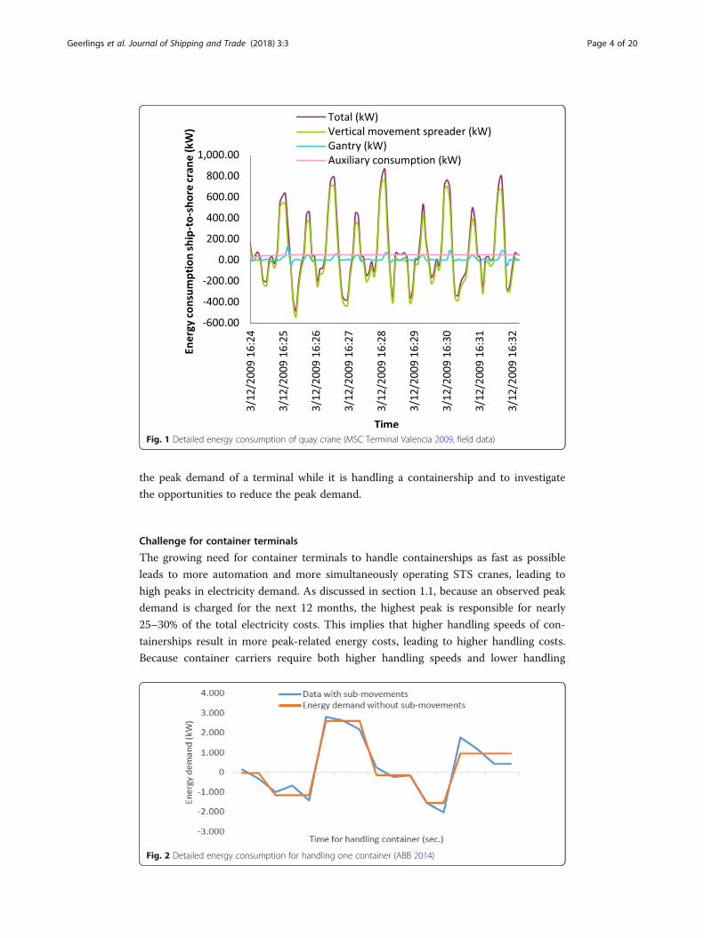
the peak demand of a terminal while it is handling a containership and to investigate

the opportunities to reduce the peak demand.

Challenge for container terminals

The growing need for container terminals to handle containerships as fast as possible

leads to more automation and more simultaneously operating STS cranes, leading to

high peaks in electricity demand. As discussed in section 1.1, because an observed peak

demand is charged for the next 12 months, the highest peak is responsible for nearly

25–30% of the total electricity costs. This implies that higher handling speeds of con-

tainerships result in more peak-related energy costs, leading to higher handling costs.

Because container carriers require both higher handling speeds and lower handling

Fig. 2 Detailed energy consumption for handling one container (ABB 2014)

Fig. 1 Detailed energy consumption of quay crane (MSC Terminal Valencia 2009, field data)

Geerlings et al. Journal of Shipping and Trade (2018) 3:3 Page 4 of 20

costs, terminals are confronted with a dilemma. The challenge is therefore to find op-

portunities to reduce the peak-related costs without reducing the handling speed too

much.

Relevance

Scientific relevance

The equipment at container terminals needs to be employed optimally by minimizing the

completion time for handling containers, because a vessel’s turnaround time is the key

performance indicator for terminal operators (De Koster et al. 2009; Bierwirth and Meisel

2010). In the literature, this is classified as a scheduling problem in which a number of

jobs (e.g. containers) are assigned to available resources such as cranes and vehicles trans-

porting containers between the quayside area and the stacking area. Because of the com-

plexity of container terminal operations, scheduling problems in a particular area are

investigated to simplify the scheduling of the overall terminal (Geerlings et al. 2018).

For the quayside area, quay crane scheduling determines the sequence in which the STS

cranes handle jobs and the time points at which these are performed (Kim and Park 2004;

Meisel 2009; Liang et al. 2009; Zhang and Kim 2009; Diabat and Theodorou 2014), given

different objectives and various operational constraints. Although the landside is not dir-

ectly related to the quayside operation, the yard crane scheduling of a single block (Ng

and Mak 2006; Gharehgozli et al., 2014a; Gharehgozli et al., 2014b) and of multiple blocks

(He et al. 2010; Chen and Langevin 2011) have been studied in order to improve the oper-

ational efficiency of the stacking area. Cao et al. (2010) consider the integrated scheduling

of the quayside transport area and the stacking area. Furthermore, the quayside area, the

quayside transport area, and the stacking area together account for the transport of con-

tainers between the vessel and the stack, and therefore the integrated scheduling of these

three areas has been investigated (Meersmans and Wagelmans 2001; Chen et al. 2007;

Meier and Schumann 2007; Lau and Zhao 2008; Meisel (2009); Chen et al. 2013). In gen-

eral, one can conclude from this literature review that the equipment scheduling problem

aims at minimizing the completion time of all jobs in order to reduce vessel turnaround

time. Scheduling problems are mainly concerned with productivity improvement without

any consideration of creating energy efficiency at terminals.

Previous research on the energy consumption of container terminals (Van der Voet 2008;

Geerlings and van Duin 2011; Van Duin and Geerlings 2011) does not provide a

visualization of the peak demand of container terminals or STS cranes. The current re-

search makes two contributions to science.

1. The first scientific contribution is the development of an energy consumption

model that can show energy demand over time (in kW/s). Over recent years, many

studies have been undertaken on the energy efficiency of container terminals. The

models presented in these studies try to describe the total energy consumption over

a given time interval (mostly in kWh per year). However, to visualize the peak

demand of container terminals, and in particular of STS cranes, a more advanced

model needs to be developed. This consumption model can also be applied to

visualize the energy demand of other types of cranes in different industries.

Geerlings et al. Journal of Shipping and Trade (2018) 3:3 Page 5 of 20

2. The second contribution is to present rules of operation that contribute to the

reduction of peak demand at container terminals and to test these rules of

operation by undertaking a case study to show the opportunities for peak shaving

the energy demand of STS cranes.

Although we have observed in literature that dividing the whole process into

sub-planning processes can lead to undesirable results and sub-optimal solutions

(Meier and Schumann 2007), the research focus is here mainly at the quay crane

scheduling to identify whether energy and costs savings can be obtained. If the re-

search shows significant savings the next step can be made by integrating the yard

crane management.

Business relevance

The size of containerships is increasing continuously. The newest generation is able

to carry almost 20,000 TEU. Container terminals are under high pressure to handle

ships as fast as possible against a low price, to improve their competitive position.

However, when more and more STS cranes are simultaneously executing a lifting

movement, peak demand and energy-related costs increase. For an intermediate

container terminal with eight STS quay cranes, the peak-related costs can account

for up to 25–30% of total energy costs. The energy consumption model and rules

of operation developed show the opportunities for container terminals to reduce

these peak-related costs, while monitoring the consequences for handling time.

This could save a terminal tens of thousands of euros per year.

Methodology

The research is executed in three different stages:

1. First, an extensive literature review is conducted on the container market and in

particular STS crane operations. This leads to a better understanding of the

problem and shows the importance of reducing the peak energy demand of STS

cranes;

2. Based on the knowledge acquired, an energy consumption model is developed by

introducing a conceptual model and a final consumption model (mathematical

formula).

3. The conceptual model is applied to a container terminal, so rules of operation can

be tested quantitatively on their ability to reduce peak energy demand. The

simulation model is developed in a discrete-event environment, with the Simio soft-

ware package (Simio, 2015). The discrete modeling approach enables the modeler to

model the

containers as passive objects with a predefined behavior and to visualize the energy

demand per second, as time continues on the basis of the occurrence of events.

Other environments, like system dynamics or agent-based modeling, do not operate

in all of these aspects. The discrete environment has been applied in earlier re-

search, for

example to model rail operations (Caballini et al. 2014), to model the time duration

of handling activities (Cartenì and De Luca 2011), to model and test several

Geerlings et al. Journal of Shipping and Trade (2018) 3:3 Page 6 of 20

container stacking algorithms (Borgman et al. 2010), and to model the container

flows within container terminals (Alessandri et al. 2007; Alessandri et al. 2008).

Energy consumption modelConceptual model

The energy consumption of STS cranes is highly dependent on the different movements

made by the crane. In total, six different general movements can be distinguished:

1. Moving spreader from quay to ship;

2. Lowering spreader at ship side;

3. Hoisting spreader at ship side;

4. Gantry (i.e. horizontal) movement from ship to shore;

5. Lowering spreader at quay side;

6. Hoisting spreader at quay side.

Each of these movements has its own energy consumption specifications. In

addition to these different movements, it is important to include the auxiliary energy

consumption. The auxiliary consumption is a fixed energy demand per hour, needed

to keep the pressure on the crane and for equipment in the cabin and engine room.

The auxiliary consumption is rather constant over time because the quay cranes are

not turned off while in idle or off-shift state.

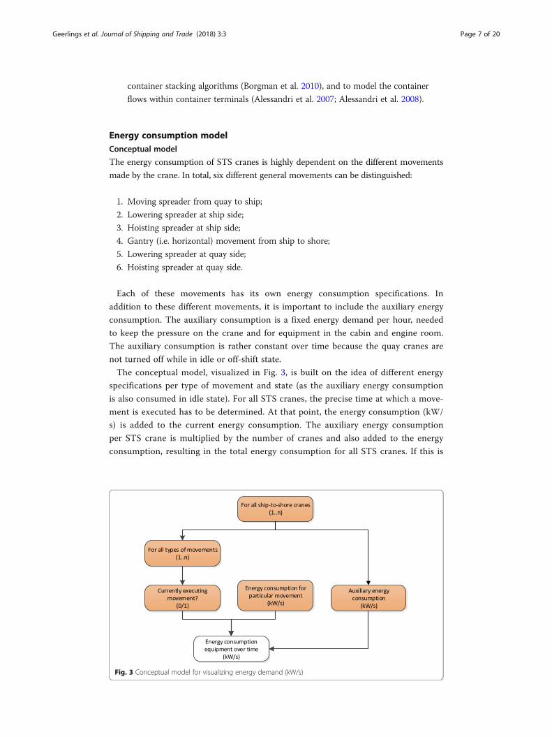
The conceptual model, visualized in Fig. 3, is built on the idea of different energy

specifications per type of movement and state (as the auxiliary energy consumption

is also consumed in idle state). For all STS cranes, the precise time at which a move-

ment is executed has to be determined. At that point, the energy consumption (kW/

s) is added to the current energy consumption. The auxiliary energy consumption

per STS crane is multiplied by the number of cranes and also added to the energy

consumption, resulting in the total energy consumption for all STS cranes. If this is

Fig. 3 Conceptual model for visualizing energy demand (kW/s)

Geerlings et al. Journal of Shipping and Trade (2018) 3:3 Page 7 of 20

done every second, the energy consumption can be visualized over time, enabling

the identification of peaks in energy demand.

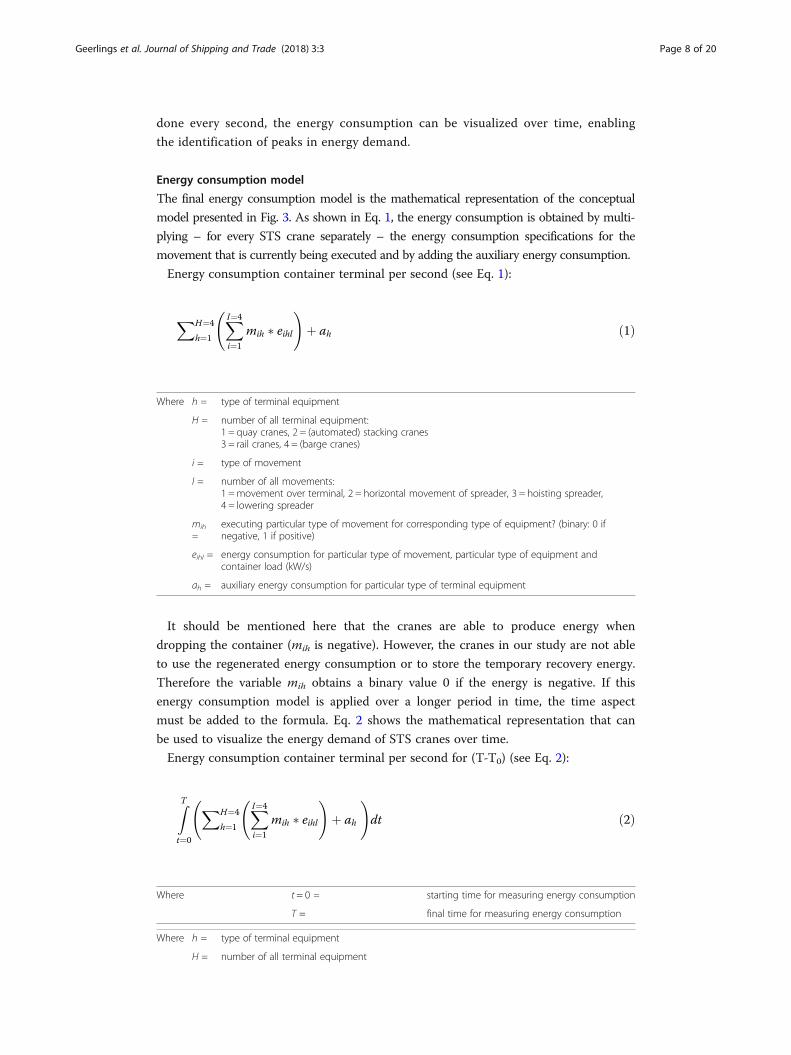
Energy consumption model

The final energy consumption model is the mathematical representation of the conceptual

model presented in Fig. 3. As shown in Eq. 1, the energy consumption is obtained by multi-

plying – for every STS crane separately – the energy consumption specifications for the

movement that is currently being executed and by adding the auxiliary energy consumption.

Energy consumption container terminal per second (see Eq. 1):

XH¼4

h¼1

XI¼4

i¼1

mih � eihl !

þ ah ð1Þ

Where h = type of terminal equipment

H = number of all terminal equipment:1 = quay cranes, 2 = (automated) stacking cranes3 = rail cranes, 4 = (barge cranes)

i = type of movement

I = number of all movements:1 =movement over terminal, 2 = horizontal movement of spreader, 3 = hoisting spreader,4 = lowering spreader

mih

=executing particular type of movement for corresponding type of equipment? (binary: 0 ifnegative, 1 if positive)

eihl = energy consumption for particular type of movement, particular type of equipment andcontainer load (kW/s)

ah = auxiliary energy consumption for particular type of terminal equipment

It should be mentioned here that the cranes are able to produce energy when

dropping the container (mih is negative). However, the cranes in our study are not able

to use the regenerated energy consumption or to store the temporary recovery energy.

Therefore the variable mih obtains a binary value 0 if the energy is negative. If this

energy consumption model is applied over a longer period in time, the time aspect

must be added to the formula. Eq. 2 shows the mathematical representation that can

be used to visualize the energy demand of STS cranes over time.

Energy consumption container terminal per second for (T-T0) (see Eq. 2):

ZT

t¼0

XH¼4

h¼1

XI¼4

i¼1

mih � eihl !

þ ah

!dt ð2Þ

Where t = 0 = starting time for measuring energy consumption

T = final time for measuring energy consumption

Where h = type of terminal equipment

H = number of all terminal equipment

Geerlings et al. Journal of Shipping and Trade (2018) 3:3 Page 8 of 20

(Continued)

i = type of movement

I = number of all movements

mih

=executing particular type of movement for corresponding type of equipment? (binary: 0 ifnegative, 1 if positive)

eihl = energy consumption for particular type of movement, particular type of equipment andcontainer load (kW/s)

ah = auxiliary energy consumption for particular type of equipment

The energy consumption model is not only suitable for visualizing the energy demand

of STS cranes; it can also be used for other crane operations at container terminals (e.g.

automated stacking cranes and rail cranes), and even in different type of industries where

cranes are used (e.g. factories or building sites).

Application of consumption modelDevelopment of simulation model

A discrete-event simulation model is constructed to apply the consumption model. When

a containership arrives and is berthed, the terminal’s quay cranes are able to start handling

containers immediately. The quay cranes take the containers through six main processes

(i.e. movements, see Fig. 4):

– Moving spreader horizontally from quay (idle position) to ship;

– Lowering spreader above ship to get a container;

– Lifting spreader and container from ship;

– Moving spreader and container horizontally from ship to quay side;

– Lowering spreader and container to terminal truck on quay side;

– Lifting spreader from quay (to idle position).

Every movement is divided into two or three sub-movements to give a more detailed out-

come of the energy demand. For each movement, a container has its own process times

and corresponding energy consumption specifications (ABB 2014). After the quay crane

processes the container through all movements, the container is picked up by a terminal

truck, bringing the container to the stacking area. Because the terminal trucks are diesel-

powered, this process does not influence the peak electricity demand. For each crane, all 18

processes can be observed in the screen views of the simulation model (see Fig. 5a and b).

The model is able to generate the following relevant output:

– Energy consumption per second (kW/s);

– Handling time for containers (seconds);

– Number of active quay cranes;

– Number of lifting quay cranes;

– Number of containers paused and their average pausing time (due to limitations

imposed by the rules of operation).

In Fig. 5a/b, a 3D/2D view of the simulation model is given. Here, eight quay cranes are

transporting the containers (red triangles) through the different (sub)movements. Each

Geerlings et al. Journal of Shipping and Trade (2018) 3:3 Page 9 of 20

Fig. 4 Main processes of the simulation model

Geerlings et al. Journal of Shipping and Trade (2018) 3:3 Page 10 of 20

sub-movement is depicted as following an activity block. The activity block takes some

operational time and consumes/produces some energy according the specifications. The

auxiliary equipment is also modeled because the cranes cannot operate on their own and

need additional vehicles to move the containers to the stack. The results of the simulation

model are verified with real data and by expert opinion (ABB 2014).

Rules of operation

The rules of operation that are implemented need to be seen as process improvements

to reduce the peak demand for STS cranes. In total, two rules of operation are

implemented in the simulation model to test their impact on peak demand and

handling time:

Restrict number of lifting quay cranesThe first rule of operation restricts the number of simultaneously lifting quay cranes

because the lifting movements are the most energy-intensive movements (see section 2.2).

Fig. 5 a 3D–Screen view of simulation model where each process-step (see Fig. 4) is modelled. b 2D–screenshotof simulation model, running for an eight-crane terminal where each process-step (see Fig. 4) is modelled

Geerlings et al. Journal of Shipping and Trade (2018) 3:3 Page 11 of 20

When, for example, maximally four of the eight STS cranes are allowed to lift simultan-

eously, some cranes may need to stop operating temporarily, waiting until one of the other

cranes finishes its lifting movement.

Restrict maximal energy demandThe second rule of operation restricts the maximal energy demand per second. Before

starting a new movement, every STS crane requests the energy that it is expecting to

consume (depending on the type of movement and container load). On the basis of

this expected consumption, the simulation model looks at whether this demand is

available. If not, the crane is asked to pause until there is enough demand left to start

the movement.

Validation of simulation model

The rules of operation are applied for two types of container terminals (six and eight

STS cranes) and a yearly throughput of 1.6 million TEU. The base scenario of the

simulation model is executed with the standard specifications of the container

terminal. This means that all eight quay cranes are handling containers, without any

restrictions on the number of simultaneously lifting quay cranes or on maximum

energy demand per second. The base scenario is run with 10 replications (more than

the minimum desired eight replications, as calculated in the last sub-section). The time

span is one week. During this week, 19 containerships arrive with a total of 20,114

TEU. Without implementation of one of the rules of operation, the peak demand is

19,230 W and peak-related energy costs are €518,000, based on the tariff of Dutch grid

operator Stedin (2014). The average maximum energy demand of all replications is

19,177 kW, with a minimum of 18,063 kW and a maximum of 20,004 kW. The corre-

sponding half width is 364.4 kW. The handling time of all containers is 1857 min,

which is 31.0 h.

The model is validated on three important aspects: container load, observed peak

demand, and handling time. All three aspects are discussed below.

Container load

Each container load (0–100%) has its own pre-defined energy specifications (kW/s).

Multiplied by the operation times per sub-movement, the total energy consumption

for a container can be determined and compared with real data. The result is that the

maximum difference in energy consumption is 0.9%. For most container loads, the

difference is not larger than 0.2%. Because the different container loads do not appear

in the same proportion, the difference is multiplied by their appearance distribution

(container mix). The result is a weighted difference of 0.26% (see Table 1), which

might not be considered significant to the energy consumption results. The influence

on the energy peak is difficult to calculate however, because it depends on the current

container mix, which is changing continuously in the simulation model.

Peak demand

If the peak demand of the simulation (base scenario with eight lifting quay cranes and

no restriction on the maximum energy demand per second) is compared, the peak

demand lies around 20,000 kW. This is consistent with data for a terminal with eight

Geerlings et al. Journal of Shipping and Trade (2018) 3:3 Page 12 of 20

quay cranes (ABB 2014); this validates the outcome of the simulation model on this

aspect.

Handling time

The total run time for the base scenario is 171.0 h (one week plus three hours extra

run time). The quay cranes are operating 18.0% of the time (half width 0.5%), which is

30.8 h. In this time frame, 10,057 containers are handled. If eight quay cranes are

operating, this results in a handling time of 88.1 s/container.

The theoretical (weighted) handling time of a container (based on the appearance of

each container load) is 91.4 s/container, a difference of 3.3 s (3.6%). This difference

could be explained by random distribution of process times for engaging the container

in the simulation model, whereas the theoretical handling time makes use of standard

process times instead of a distribution.

ResultsResults for limiting number of lifting quay cranes

If the number of lifting STS cranes is reduced, the peak demand decreases, as shown in

Fig. 6. What is striking is that the handling time does not increase in the same

proportion. A reduction to four lifting cranes leads to an extra handling time of 0.37%

(i.e. less than half a minute per hour). The handling time is not impacted that much

Table 1 Weighted difference for difference in energy demand

Container load Container mix Difference Weighted difference

0% 12.5% 0.00% 0.00%

20% 32.0% 0.20% 0.06%

30% 11.1% 0.35% 0.04%

40% 11.4% 0.16% 0.02%

50% 13.6% 0.00% 0.00%

60% 13.6% 0.90% 0.12%

70% 3.3% 0.42% 0.01%

80% 1.6% 0.21% 0.00%

90% 0.6% 0.00% 0.00%

100% 0.3% 0.00% 0.00%

Total weighted average 0.26%

Fig. 6 Relation between peak demand and handling time when the number of lifting cranes is restricted

Geerlings et al. Journal of Shipping and Trade (2018) 3:3 Page 13 of 20

because of the fact that the maximum peak demand with eight cranes (around

19,000 kW) occurs only briefly. As shown by Fig. 7, for a peak demand of 19,000 kW,

an energy demand of more than 9000 kW occurs only 1.1% of the time. Most of the

time, the energy demand is lower than 9000 kW.

As can be concluded from Fig. 6, restricting the number of simultaneously lifting

quay cranes has a positive influence on reducing peak demand. If one looks at the

impact on cost savings on the one hand and handling time on the other hand, one can

see the most cost-effective scenario (i.e. yearly savings per extra second handling time)

and the total cost reduction against a particular extra handling time.

The optimal cost-effective implementation is to reduce the number of lifting quay

cranes to six (eight-crane terminal) or five (six-crane terminal) as can be seen in Fig. 8.

In these cases, the savings per extra second handling time are higher than for other

scenarios.

If one looks at the total yearly savings against an extra handling time of less than

1.0%, the number of quay cranes can be limited even more. In the case of an eight-

crane terminal, this could result in a reduction to four lifting cranes. This saves

€195,000, which is 39% of the peak-related costs. For a six-crane terminal, this would

result in a reduction to three lifting cranes, which saves €155,000 (reducing total peak

demand costs by 38%).

Results for limiting maximum energy demand

To limit the maximum energy demand per second, the relation between the maximum

allowed energy demand and handling time (see Fig. 9) is comparable to the situation

where the number of simultaneously lifting STS cranes is limited. The maximum

energy demand can be reduced by almost 50% (from 19,000 kW to 9000 kW), while

the handling time increases by 0.1%. Only by restricting the energy demand too much

(to less than 6000 kW) does the handling time increase by 3–45%.

Restricting the maximum allowed energy demand has a positive influence on

reducing terminals’ peak demand. The influence on handling time is only minimal

when the allowed energy demand is reduced by approximately less than 50%, whereas

it enables terminals to reduce their peak-related energy costs hugely.

Fig. 7 Frequency (per 0.1 s) per energy demand interval

Geerlings et al. Journal of Shipping and Trade (2018) 3:3 Page 14 of 20

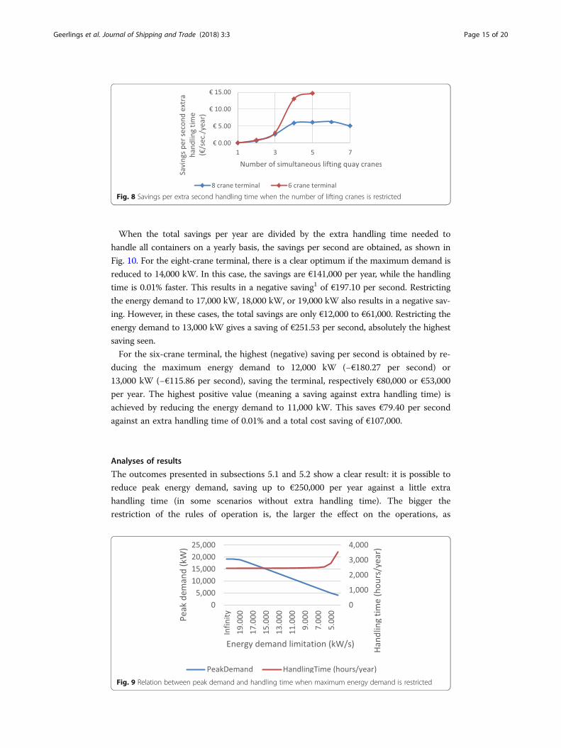
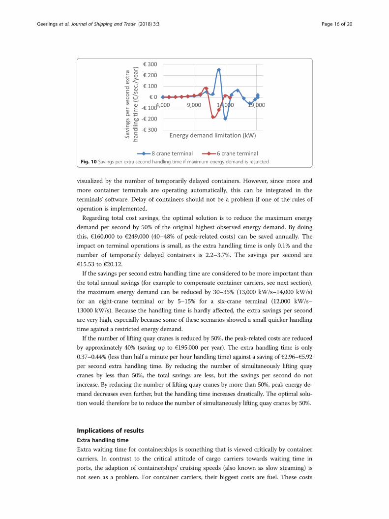
When the total savings per year are divided by the extra handling time needed to

handle all containers on a yearly basis, the savings per second are obtained, as shown in

Fig. 10. For the eight-crane terminal, there is a clear optimum if the maximum demand is

reduced to 14,000 kW. In this case, the savings are €141,000 per year, while the handling

time is 0.01% faster. This results in a negative saving1 of €197.10 per second. Restricting

the energy demand to 17,000 kW, 18,000 kW, or 19,000 kW also results in a negative sav-

ing. However, in these cases, the total savings are only €12,000 to €61,000. Restricting the

energy demand to 13,000 kW gives a saving of €251.53 per second, absolutely the highest

saving seen.

For the six-crane terminal, the highest (negative) saving per second is obtained by re-

ducing the maximum energy demand to 12,000 kW (−€180.27 per second) or

13,000 kW (−€115.86 per second), saving the terminal, respectively €80,000 or €53,000

per year. The highest positive value (meaning a saving against extra handling time) is

achieved by reducing the energy demand to 11,000 kW. This saves €79.40 per second

against an extra handling time of 0.01% and a total cost saving of €107,000.

Analyses of results

The outcomes presented in subsections 5.1 and 5.2 show a clear result: it is possible to

reduce peak energy demand, saving up to €250,000 per year against a little extra

handling time (in some scenarios without extra handling time). The bigger the

restriction of the rules of operation is, the larger the effect on the operations, as

Fig. 8 Savings per extra second handling time when the number of lifting cranes is restricted

Fig. 9 Relation between peak demand and handling time when maximum energy demand is restricted

Geerlings et al. Journal of Shipping and Trade (2018) 3:3 Page 15 of 20

visualized by the number of temporarily delayed containers. However, since more and

more container terminals are operating automatically, this can be integrated in the

terminals’ software. Delay of containers should not be a problem if one of the rules of

operation is implemented.

Regarding total cost savings, the optimal solution is to reduce the maximum energy

demand per second by 50% of the original highest observed energy demand. By doing

this, €160,000 to €249,000 (40–48% of peak-related costs) can be saved annually. The

impact on terminal operations is small, as the extra handling time is only 0.1% and the

number of temporarily delayed containers is 2.2–3.7%. The savings per second are

€15.53 to €20.12.

If the savings per second extra handling time are considered to be more important than

the total annual savings (for example to compensate container carriers, see next section),

the maximum energy demand can be reduced by 30–35% (13,000 kW/s–14,000 kW/s)

for an eight-crane terminal or by 5–15% for a six-crane terminal (12,000 kW/s–

13000 kW/s). Because the handling time is hardly affected, the extra savings per second

are very high, especially because some of these scenarios showed a small quicker handling

time against a restricted energy demand.

If the number of lifting quay cranes is reduced by 50%, the peak-related costs are reduced

by approximately 40% (saving up to €195,000 per year). The extra handling time is only

0.37–0.44% (less than half a minute per hour handling time) against a saving of €2.96–€5.92

per second extra handling time. By reducing the number of simultaneously lifting quay

cranes by less than 50%, the total savings are less, but the savings per second do not

increase. By reducing the number of lifting quay cranes by more than 50%, peak energy de-

mand decreases even further, but the handling time increases drastically. The optimal solu-

tion would therefore be to reduce the number of simultaneously lifting quay cranes by 50%.

Implications of resultsExtra handling time

Extra waiting time for containerships is something that is viewed critically by container

carriers. In contrast to the critical attitude of cargo carriers towards waiting time in

ports, the adaption of containerships’ cruising speeds (also known as slow steaming) is

not seen as a problem. For container carriers, their biggest costs are fuel. These costs

Fig. 10 Savings per extra second handling time if maximum energy demand is restricted

Geerlings et al. Journal of Shipping and Trade (2018) 3:3 Page 16 of 20

can be reduced by adapting the ship’s speed: a reduction to 80% saves 60% of fuel costs,

and a reduction to 60% saves 90% of fuel costs (Weismann 2010). A market survey has

shown that 75% of the surveyed liners and carriers apply slow steaming in order to

save bunker costs (Seatrade Global 2014). Because fuel costs are so high, container

carriers operate more efficiently by sailing at lower speeds. In this regard, the extra

travel time is compensated by fuel savings.

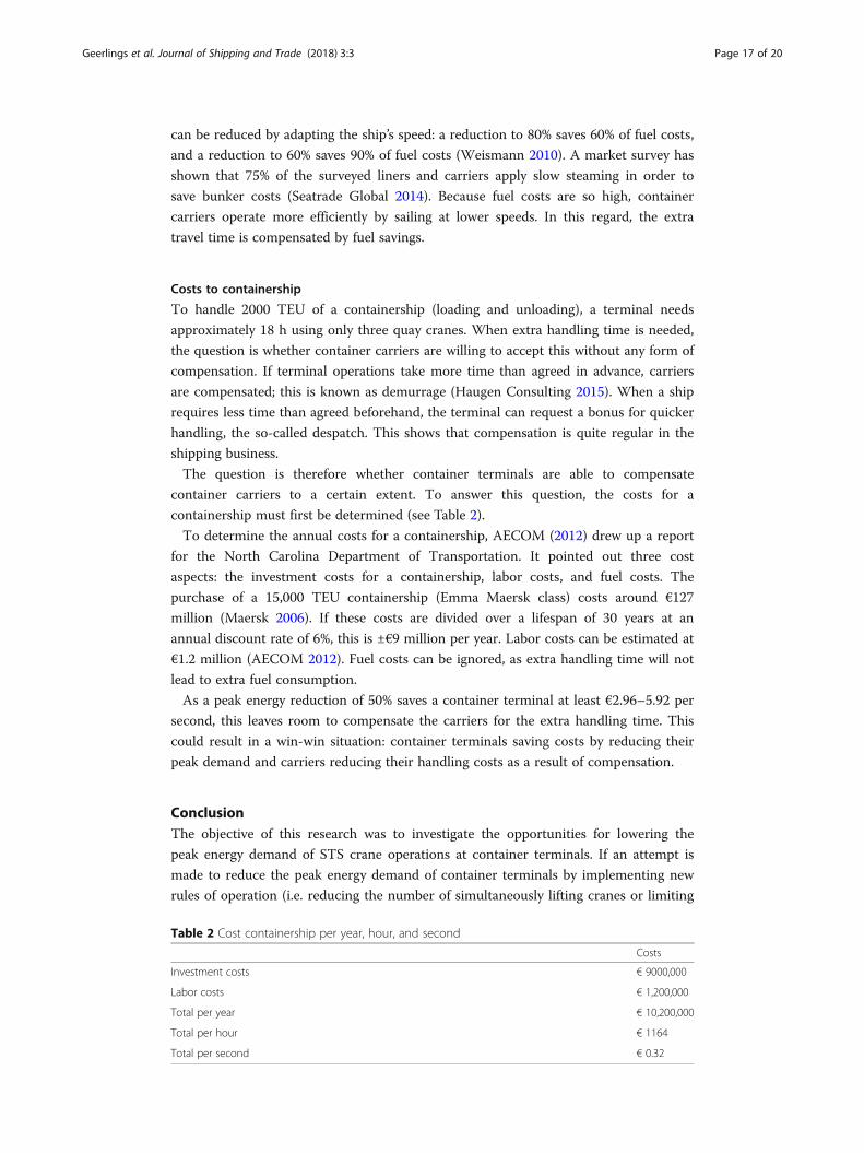
Costs to containership

To handle 2000 TEU of a containership (loading and unloading), a terminal needs

approximately 18 h using only three quay cranes. When extra handling time is needed,

the question is whether container carriers are willing to accept this without any form of

compensation. If terminal operations take more time than agreed in advance, carriers

are compensated; this is known as demurrage (Haugen Consulting 2015). When a ship

requires less time than agreed beforehand, the terminal can request a bonus for quicker

handling, the so-called despatch. This shows that compensation is quite regular in the

shipping business.

The question is therefore whether container terminals are able to compensate

container carriers to a certain extent. To answer this question, the costs for a

containership must first be determined (see Table 2).

To determine the annual costs for a containership, AECOM (2012) drew up a report

for the North Carolina Department of Transportation. It pointed out three cost

aspects: the investment costs for a containership, labor costs, and fuel costs. The

purchase of a 15,000 TEU containership (Emma Maersk class) costs around €127

million (Maersk 2006). If these costs are divided over a lifespan of 30 years at an

annual discount rate of 6%, this is ±€9 million per year. Labor costs can be estimated at

€1.2 million (AECOM 2012). Fuel costs can be ignored, as extra handling time will not

lead to extra fuel consumption.

As a peak energy reduction of 50% saves a container terminal at least €2.96–5.92 per

second, this leaves room to compensate the carriers for the extra handling time. This

could result in a win-win situation: container terminals saving costs by reducing their

peak demand and carriers reducing their handling costs as a result of compensation.

ConclusionThe objective of this research was to investigate the opportunities for lowering the

peak energy demand of STS crane operations at container terminals. If an attempt is

made to reduce the peak energy demand of container terminals by implementing new

rules of operation (i.e. reducing the number of simultaneously lifting cranes or limiting

Table 2 Cost containership per year, hour, and second

Costs

Investment costs € 9000,000

Labor costs € 1,200,000

Total per year € 10,200,000

Total per hour € 1164

Total per second € 0.32

Geerlings et al. Journal of Shipping and Trade (2018) 3:3 Page 17 of 20

the maximum energy demand), it is shown that the peak can be reduced by 50% while

impacting the handling time less than half a minute per hour. A cost reduction of 50%

saves a container terminal with eight quay cranes and a throughput of 1.6 million TEU

up to €275,000 per year.

Besides the positive effect of cost savings, the reduction of peak energy demand has

consequences for the handling time. In most scenarios (depending on how much the

number of simultaneously lifting cranes and energy demand per second is limited), the

extra handling time would be less than half a minute per hour. The question is whether

container carriers are willing to accept extra handling time. Container terminals need

to be prepared to negotiate with container carriers about some sort of compensation.

This could be financial, but might also relate to extra service (e.g. free electricity power

for ships while berthed) or sustainability agreements. Irrespective of how costs are

allocated, this research has shown that container terminals can reduce their peak-

related energy costs by managing their energy consumption in a smarter way.

Next research step is to study the integrated scheduling of the quayside area, the

quayside transport area, and the stacking area together in order to evaluate the

consequences of the new crane scheduling for the costs savings and container handling

times (Wong and Kozan 2006; Boer and Saanen 2014).

Endnotes1The negative cost saving per second is actually a positive result, because the

handling time for this scenario is lower than for the standard situation, meaning that

the cost savings (positive result) are divided by a negative extra handling time (i.e. less

handling time).

AcknowledgementsOn 7 June 2015, Robert Heij, co-author of this paper, passed away after 1 year of illness. Robert suffered from an aggressiveform of cancer. During his illness, he was determined to complete his thesis and graduated. Robert’s work (Heij 2015) wasexcellent, and he was nominated for the SmartPort ‘best thesis award’ in Rotterdam. On June 11, 1 day before his funeral, hewas announced as the winner. We promised to continue his work. Therefore, in tribute to his memory, the other co-authorsof this paper, Harry Geerlings and Ron van Duin, now dedicate this paper to Robert Heij.

Fundingthere is no funding body in the design of the study and collection, analysis, and interpretation of data and in writingthe manuscript should be declared.

Authors’ contributionsThere is no specific individual contributions of authors to the manuscript. All authors read and approved the finalmanuscript.

Competing interestsThe authors declare that they have no competing interests.

Publisher’s NoteSpringer Nature remains neutral with regard to jurisdictional claims in published maps and institutional affiliations.

Author details1Erasmus University Rotterdam, Erasmus School of Social and Behavioural Sciences/ Erasmus Smart Port, P.O. box 1738,3000 DR Rotterdam, The Netherlands. 2Delft University of Technology, Faculty of Technology, Policy and Management,Delft, The Netherlands. 3Rotterdam University of Applied Sciences, Rotterdam, The Netherlands.

Received: 25 August 2017 Accepted: 7 February 2018

ReferencesABB, 2014. Data Quay Cranes. Internal Document ABB B.V. Marine Rotterdam (for internal use only)AECOM, 2012. Vessel Size vs. Cost. AECOM, Los Angeles

Geerlings et al. Journal of Shipping and Trade (2018) 3:3 Page 18 of 20

Alessandri A, Cervellera C, Cuneo M, Gaggero M, Soncin G (2008) Modeling and feedback control for resourceallocation and performance analysis in container terminals. IEEE Trans Intell Transp Syst 9(4):601–614

Alessandri A, Sacone S, Siri S (2007) Modelling and optimal receding-horizon control of maritime container terminals. JMath Model Algorithms 6(1):109–133

APM Terminals, 2014. Terminal Information.Bierwirth C, Meisel F (2010) A survey of berth allocation and quay crane scheduling problems in container terminals.

Eur J Oper Res 202(3):615–627.Boer CA, Saanen YA (2014) Plan validation for container terminals. In: Tolk A, Diallo SY, Ryzhov IO, Yilmaz L, Buckley S,

Miller JA (eds) Proceedings of the 2014 winter simulation conference, at savannah, GA, USA, pp 1783–1794Borgman B, van Asperen E, Dekker R (2010) Online rules for container stacking. OR Spectr 32(3):687–716Bortfeldt A, Gehring H (2001) A hybrid genetic algorithm for the container loading problem. Eur J Oper Res 131(1):143–161Caballini C, Pasquale C, Sacone S, Siri S (2014) An event-triggered receding-horizon scheme for planning rail operations

in maritime terminals. IEEE Trans Intell Transp Syst 15(1):365–375Cao JX, Lee D, Chen JH, Shi Q (2010) The integrated yard truck and yard crane scheduling problem: benders’

decomposition-based methods. Transp Res E 46(3):344–353Cartenì A, De Luca S (2011) Tactical and strategic planning for a container terminal: modelling issues within a discrete

event simulation approach. Simul Model Pract Theory 21(1):123–145Chen L, Bostel N, Dejax P, Cai J, Xi L (2007) A tabu search algorithm for the integrated scheduling problem of container

handling systems in a maritime terminal. Eur J Oper Res 181(1):40–58Chen L, Langevin A (2011) Multiple yard cranes scheduling for loading operations in a container terminal. Eng Optim

43(11):1205–1221Chen L, Langevin A, Lu Z (2013) Integrated scheduling of crane handling and truck transportation in a maritime

container terminal. Eur J Oper Res 225(1):142–152Clarksons, 2015. Clarksons, the heart of global shipping. Retrieved from Containers: http://www.clarksons.com/services/

broking/containers/De Koster R, Balk B, van Nus W (2009) On using DEA for benchmarking container terminals. Int J Oper Prod Manag

29(11):1140–1155Dekker R, Voogd P, van Asperen E (2006) Advanced methods for container stacking. OR Spectr 28:563–586Diabat A, Theodorou E (2014) An integrated quay crane assignment and scheduling problem. Comput Ind Eng 73:115–123Eugen R, Şerban R, Augustin R, Ştefan B (2014) Transshipment modelling and simulation of container port terminals.

Adv Mater Res 837:786–791Geerlings H, Kuipers B, Zuidwijk R (2018) Port and networks; strategies, operations and perspectives. Routledge,

AbingdonGeerlings H, van Duin R (2011) A new method for assessing CO2-emissions from container terminals: a promising

approach applied in Rotterdam. J Clean Prod 19(6–7), 657–666Gharehgozli AH, Laporte G, Yu Y, De Koster R (2014a) Scheduling twin yard cranes in a container block. Transp Sci

49(3):686–705Gharehgozli AH, Yu Y, de Koster R, Udding JT (2014b) An exact method for scheduling a yard crane. Eur J Oper Res

235(2):431–447Grunow M, Günther H, Lehmann M (2005) Dispatching multi-load AGVs in highly automated seaport container

terminals. In: Günther H, Kim K (eds) Container terminals and automated transport systems. Springer, Berlin, pp231–258

Haugen Consulting, 2015. What Is Demurrage? Retrieved from http://www.haugenconsulting.com/resources/what-is-demurrage/

He J, Chang D, Mi W, Yan W (2010) A hybrid parallel genetic algorithm for yard crane scheduling. Transp Res E 46(1):136–155Heij, R., 2015. Opportunities for peak shaving electricity consumption at container terminals. Applying new rules

of operation to achieve a more balanced electricity consumption. Master's thesis. Delft University ofTechnology, Delft

Imai A, Sasaki K, Nishimura E, Papadimitriou S (2006) Multi-objective simultaneous stowage and load planning for acontainer ship with container rehandle in yard stacks. Eur J Oper Res 171(2):373–389

Kim KP, Park YM (2004) A crane scheduling method for port container terminals. Eur J Oper Res 156(3):752–768Lau HYK, Zhao Y (2008) Integrated scheduling of handling equipment at automated container terminals. Int J Prod

Econ 112(2):665–682Liang C, Huang Y, Yang Y (2009) A quay crane dynamic scheduling problem by hybrid evolutionary algorithm for berth

allocation planning. Comput Ind Eng 56(3):1021–1028Lloyd's List, 2015. MSC Oscar becomes the world's largest boxship. Retrieved from http://www.lloydslist.com/ll/news/

article453843.eceMaersk, 2006. Emma Maersk/Container vessel specifications. Retrieved from http://www.emma-maersk.com/specification/Meersmans PJM, Wagelmans APM (2001) Effective algorithms for integrated scheduling of handling equipment at

automated container terminals, Technical report, econometric institute. Erasmus University Rotterdam, Rotterdam,The Netherlands

Meier L, Schumann R (2007) Coordination of interdependent planning systems, a case study. In: Koschke R, Herzog O,Roediger K, Ronthaler M (eds) Informatik, 2007, volume P-109 of lecture notes in informatics (LNI). Gesellschaft furInformatik, Bremen, Germany, pp 389–396

Meisel F (2009) Seaside operations planning in container terminals. Berlin. Physica-Verlag, GermanyMSC Terminal Valencia. 2009. Energy consumption quay crane.Ng WG, Mak KL (2006) Yard crane scheduling in port container terminals. Appl Math Model 29(1):263–276Port of Rotterdam, 2015. Focus-on-Vessels-in-the-port-of-rotterdam.. Retrieved from https://www.portofrotterdam.com/

sites/default/files/Focus-on-Vessels-in-the-port-of-rotterdam.pdf at 15 June 2016Seatrade Global, 2014. The economics of slow steaming. Retrieved from http://www.seatrade-maritime.com/news/

americas/the-economics-of-slow-steaming.html

Geerlings et al. Journal of Shipping and Trade (2018) 3:3 Page 19 of 20

Simio LLC., 2015. Simio Simulation Software. http://www.anylogic.com/download-free-simulation-software-for-education/?gclid=COHpw6uCyMsCFaqe2wod82IJSA

Stahlbock, R., Voß, S., 2008. Operations research at container terminals: a literature update. OR Spectrum 30(1), 1–52Stedin, 2014. Electriciteit tarieven 2014 – aansluiting en transport voor grootverbruikers. Retrieved from http://www.

stedin.net/zakelijk/~/media/files/stedin/tarieven/kv/stedin-voorbeeldnota-elektriciteit.pdf [In Dutch].Steenken D, Voß S, Stahlbock R (2004) Container terminal operation and operations research. OR, vol 26. Spectrum, pp 3–49UNCTAD. secretariat, based on Clarksons Research, Seaborne Trade Monitor, 2(5), 2015Van der Voet, M., 2008. CO2-emissie door containeroverslagprocessen in de Rotterdamse haven. Master's thesis. Delft

University of Technology, DelftVan Duin R, Geerlings H (2011) Estimating CO2-footprints of container terminal port-operations. Int J Sustain Dev Plan

6(4):459–473Weismann A (2010) Slow steaming – a viable long-lerm option? Wärtsilä Tech J 2:49–55 Retrieved from http://www.

wartsila.com/docs/default-source/Service-catalogue-files/Engine-Services-%2D-2-stroke/slow-steaming-a-viable-long-term-option.pdf?sfvrsn=0

Wilson I, Roach P (2000) Container stowage planning: a methodology for generating computerised solutions. J OperRes Soc 51(11):1248–1255

Wong, A., Kozan, E., 2006. An intergrated approach in optimising container process at seaport container terminals.Proceedings of the second international intelligent logistics systems conference 2006, 23.1-23-14

Zhang H, Kim KH (2009) Maximizing the number of dual-cycle operations of quay cranes in container terminals.Comput Ind Eng 56(3):979–992

Geerlings et al. Journal of Shipping and Trade (2018) 3:3 Page 20 of 20