Operations Research –Massimo Paolucci –DIBRIS Universityof ... didattico 2017... · Operations...
31
Transcript of Operations Research –Massimo Paolucci –DIBRIS Universityof ... didattico 2017... · Operations...
Operations Research – Massimo Paolucci – DIBRIS University of Genova
Linear Mathematical Programming (LP)
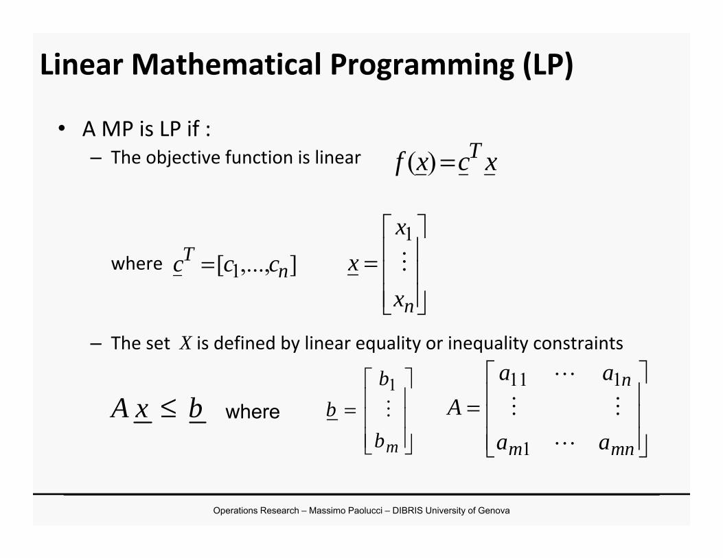
• A MP is LP if :– The objective function is linear
where
– The set X is defined by linear equality or inequality constraints
xcxf T=)(
],...,[ 1 nT ccc =
=
nx
xx
1
bxA ≤ where
=
mb
bb
1
=
mnm
n
aa
aaA
1
111
Operations Research – Massimo Paolucci – DIBRIS University of Genova
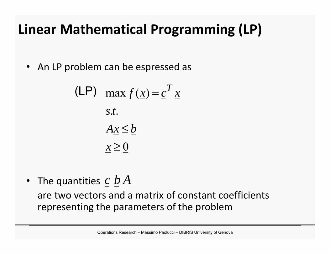
• An LP problem can be espressed as
• The quantitiesare two vectors and a matrix of constant coefficients representing the parameters of the problem
0
..)(max
≥≤
=
xbxA
tsxcxf T(LP)
Abc
Linear Mathematical Programming (LP)
Operations Research – Massimo Paolucci – DIBRIS University of Genova
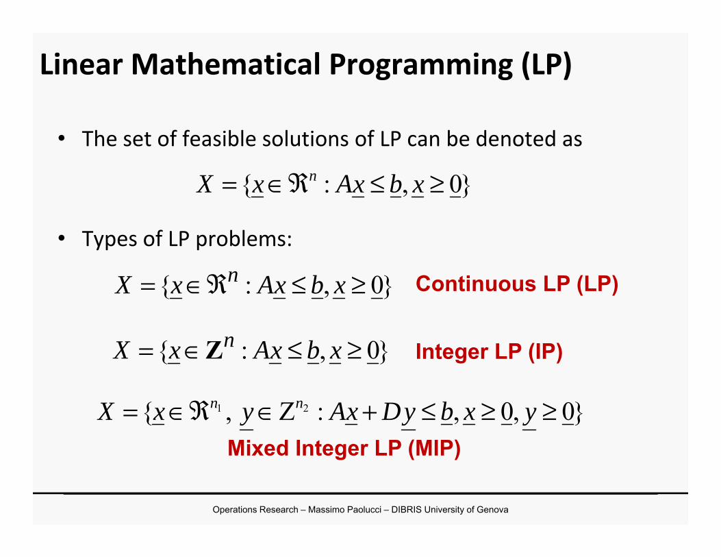
• The set of feasible solutions of LP can be denoted as
• Types of LP problems:
}0,:{ ≥≤ℜ∈= xbxAxX n
Continuous LP (LP)}0,:{ ≥≤ℜ∈= xbxAxX n
}0,:{ ≥≤∈= xbxAxX nZ
Linear Mathematical Programming (LP)
Integer LP (IP)
}0,0,:Z,{ 21 ≥≥≤+∈ℜ∈= yxbyDxAyxX nn
Mixed Integer LP (MIP)
Operations Research – Massimo Paolucci – DIBRIS University of Genova
• How can a decision problem to be modeled as a LP problem?• What corresponds to the set X?• How can we find a solution to our decision problem?
• We see these aspects considering an example ...
Linear Mathematical Programming (LP)
Operations Research – Massimo Paolucci – DIBRIS University of Genova
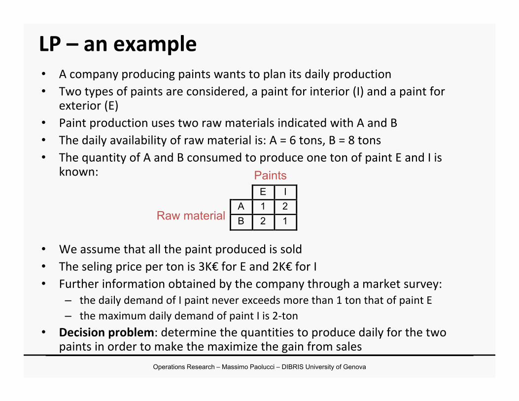
LP – an example• A company producing paints wants to plan its daily production• Two types of paints are considered, a paint for interior (I) and a paint for
exterior (E)• Paint production uses two raw materials indicated with A and B• The daily availability of raw material is: A = 6 tons, B = 8 tons• The quantity of A and B consumed to produce one ton of paint E and I is
known:E I
A 1 2B 2 1Raw material
Paints
• We assume that all the paint produced is sold• The seling price per ton is 3K€ for E and 2K€ for I• Further information obtained by the company through a market survey:
– the daily demand of I paint never exceeds more than 1 ton that of paint E – the maximum daily demand of paint I is 2-ton
• Decision problem: determine the quantities to produce daily for the two paints in order to make the maximize the gain from sales
Operations Research – Massimo Paolucci – DIBRIS University of Genova
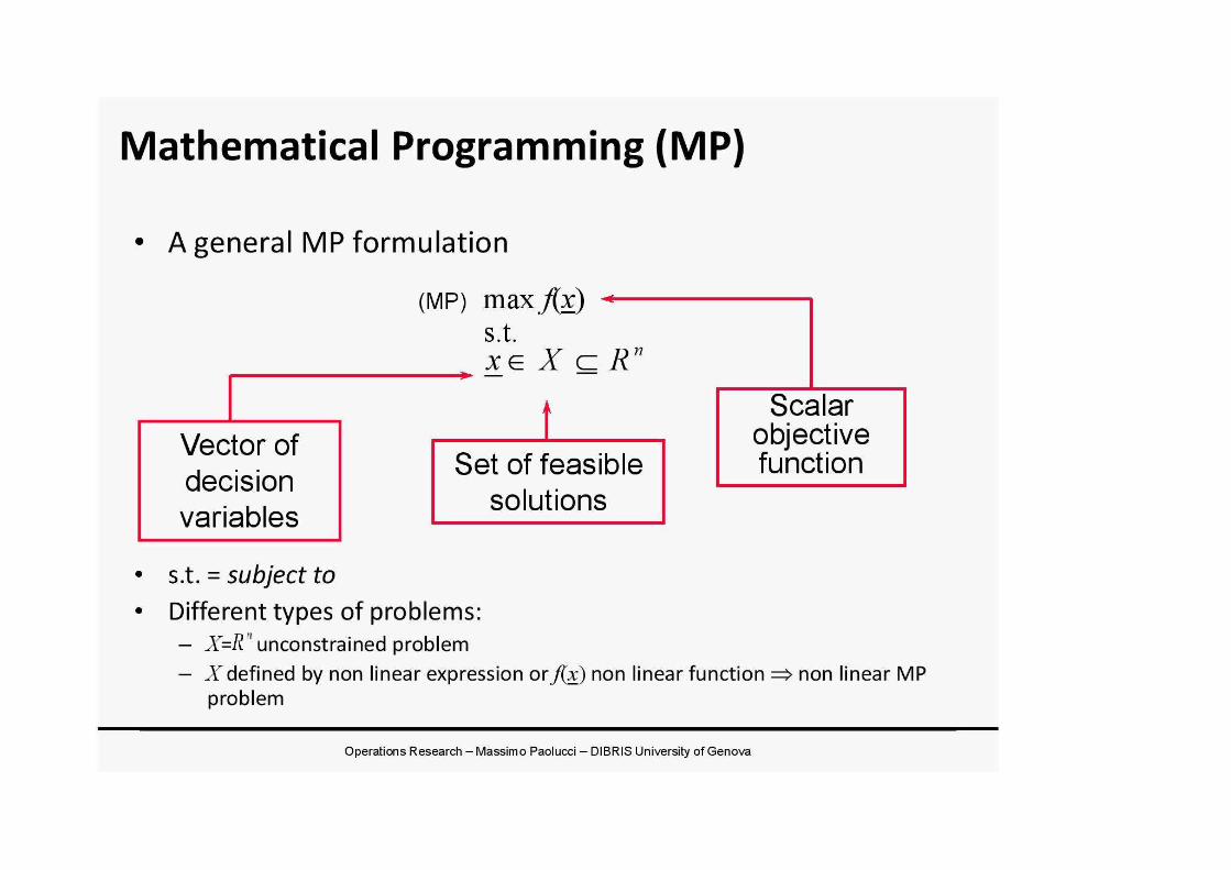
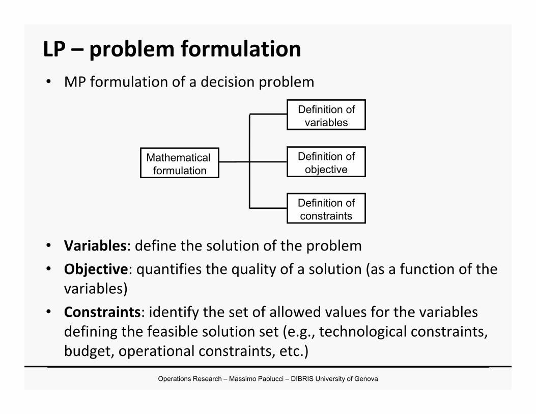
LP – problem formulation• MP formulation of a decision problem
• Variables: define the solution of the problem• Objective: quantifies the quality of a solution (as a function of the
variables)• Constraints: identify the set of allowed values for the variables
defining the feasible solution set (e.g., technological constraints, budget, operational constraints, etc.)
Mathematical formulation
Definition ofvariables
Definition ofobjective
Definition ofconstraints
Operations Research – Massimo Paolucci – DIBRIS University of Genova
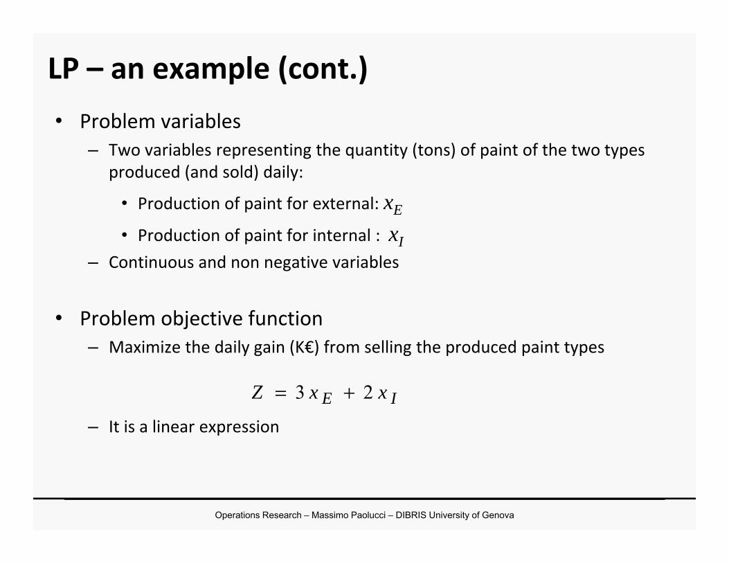
LP – an example (cont.)• Problem variables
– Two variables representing the quantity (tons) of paint of the two types produced (and sold) daily:
• Production of paint for external: xE
• Production of paint for internal : xI– Continuous and non negative variables
• Problem objective function– Maximize the daily gain (K€) from selling the produced paint types
– It is a linear expressionIE xxZ 23 +=
Operations Research – Massimo Paolucci – DIBRIS University of Genova
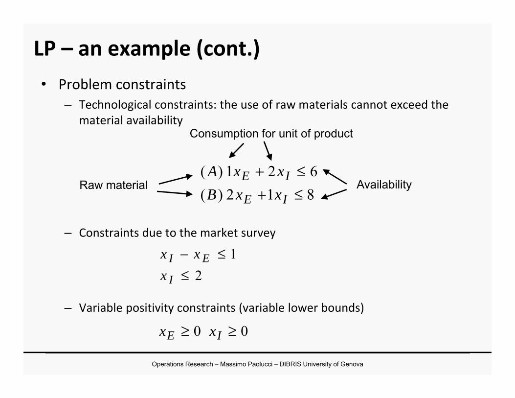
• Problem constraints– Technological constraints: the use of raw materials cannot exceed the
material availability
– Constraints due to the market survey
– Variable positivity constraints (variable lower bounds)
812)(621)(
≤+≤+
IE
IExxBxxA
Raw material Availability
Consumption for unit of product
LP – an example (cont.)
21
≤≤−
I
EIx
xx
00 ≥≥ IE xx
Operations Research – Massimo Paolucci – DIBRIS University of Genova
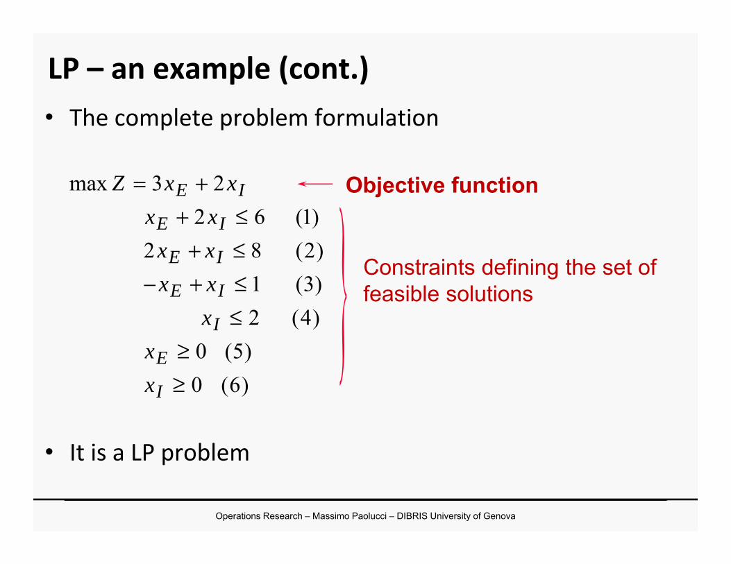
• The complete problem formulation
• It is a LP problem
)6(0)5(0
)4(2)3(1)2(82)1(62
23max
≥≥
≤≤+−≤+≤+
+=
I
E
I
IE
IE
IE
IE
xx
xxxxxxx
xxZ
Constraints defining the set of feasible solutions
Objective function
LP – an example (cont.)
Operations Research – Massimo Paolucci – DIBRIS University of Genova
8
7
6
5
4
3
2
1
1 2 3 4 5 6-1-2 xE
xI (5)
(6)(1)
(2)(3)
(4)
X
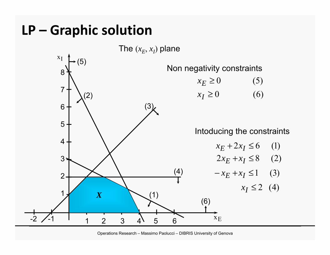
)1(62 ≤+ IE xx
The (xE, xI) plane
)6(0)5(0
≥≥
I
Exx
Non negativity constraints
Intoducing the constraints
)2(82 ≤+ IE xx)3(1≤+− IE xx)4(2≤Ix
LP – Graphic solution
Operations Research – Massimo Paolucci – DIBRIS University of Genova
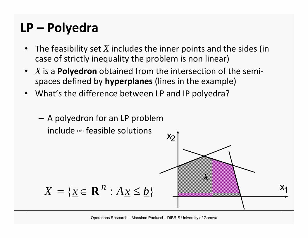
LP – Polyedra• The feasibility set X includes the inner points and the sides (in
case of strictly inequality the problem is non linear)• X is a Polyedron obtained from the intersection of the semi-
spaces defined by hyperplanes (lines in the example)• What’s the difference between LP and IP polyedra?
– A polyedron for an LP probleminclude ∞ feasible solutions
}:{ bxAxX n ≤∈= RX
x1
x2
Operations Research – Massimo Paolucci – DIBRIS University of Genova
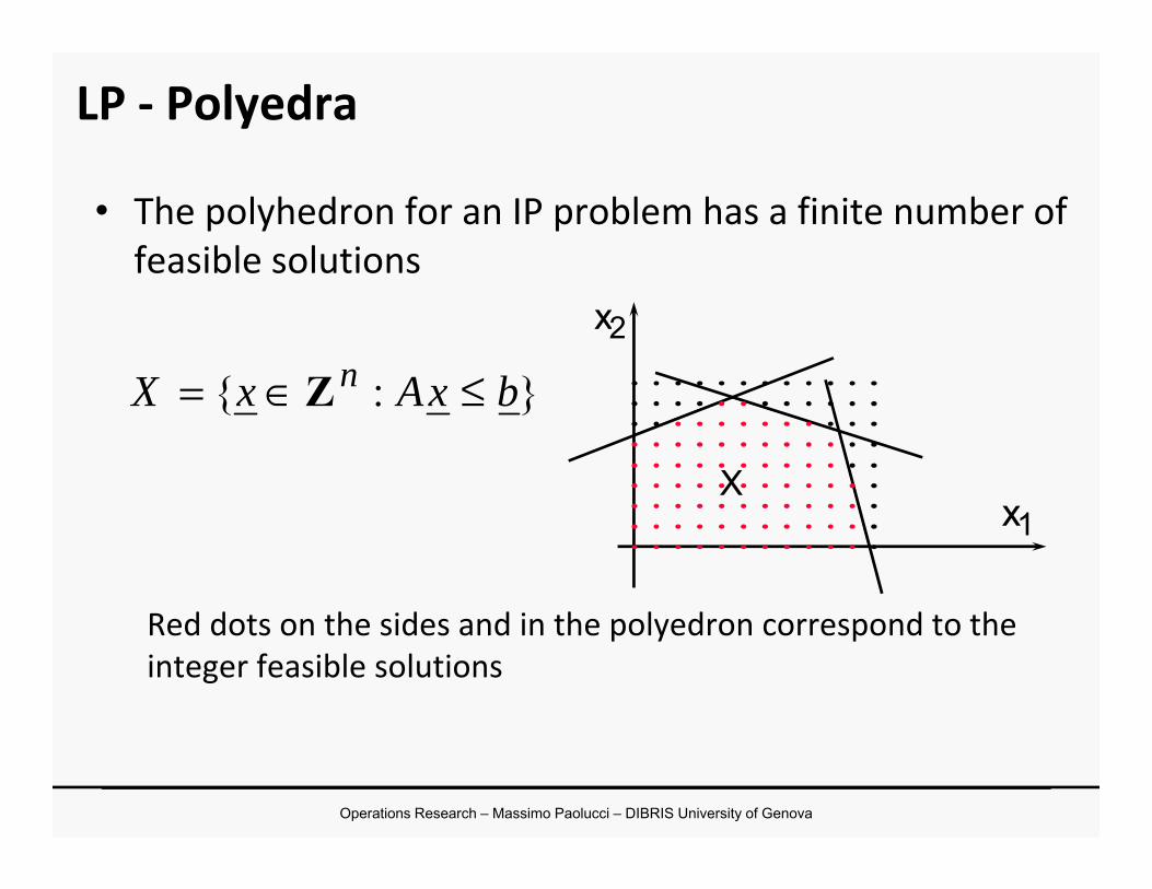
• The polyhedron for an IP problem has a finite number of feasible solutions
Red dots on the sides and in the polyedron correspond to the integer feasible solutions
}:{ bxAxX n ≤∈= Z
Xx1
x2
LP - Polyedra
Operations Research – Massimo Paolucci – DIBRIS University of Genova
1 2 3 4 5 6
1
-1-2
2
3
4(2) (3)
(4)
(1)
(5)
(6)xE
xI
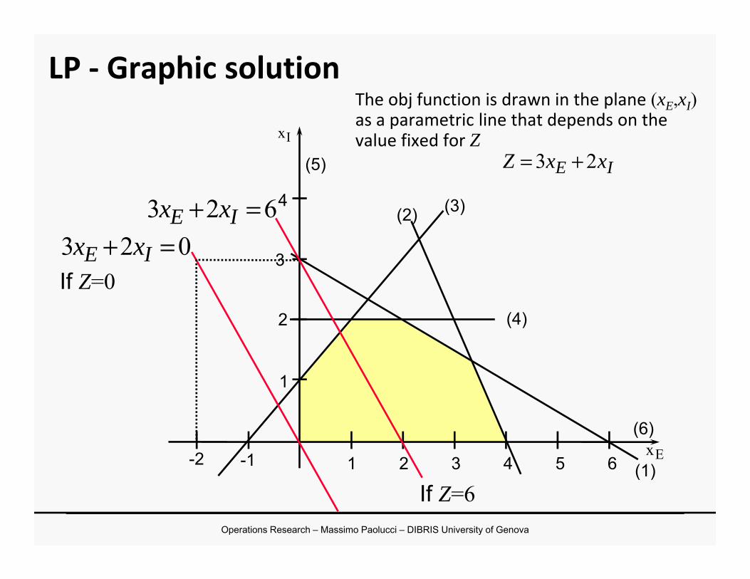
023 =+ IE xxIf Z=0
If Z=6
623 =+ IE xx
LP - Graphic solutionThe obj function is drawn in the plane (xE,xI) as a parametric line that depends on the value fixed for Z
IE xxZ 23 +=
Operations Research – Massimo Paolucci – DIBRIS University of Genova
1 2 3 4 5 6
1
-1-2
2
3
4(2) (3)
(4)
(1)
(5)
(6)xE
xI
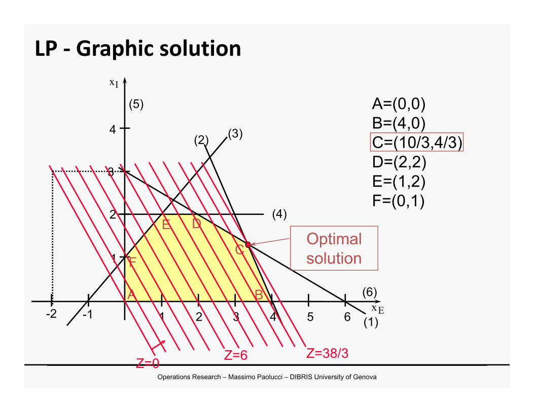
A
F
E D
B
C
A=(0,0)B=(4,0)C=(10/3,4/3) D=(2,2)E=(1,2)F=(0,1)
Z=0 Z=6 Z=38/3
Optimal solution
LP - Graphic solution
Operations Research – Massimo Paolucci – DIBRIS University of Genova
1 2 3 4 5 6
1
-1-2
2
3
4(2) (3)
(4)
(1)
(5)
(6)xE
xI
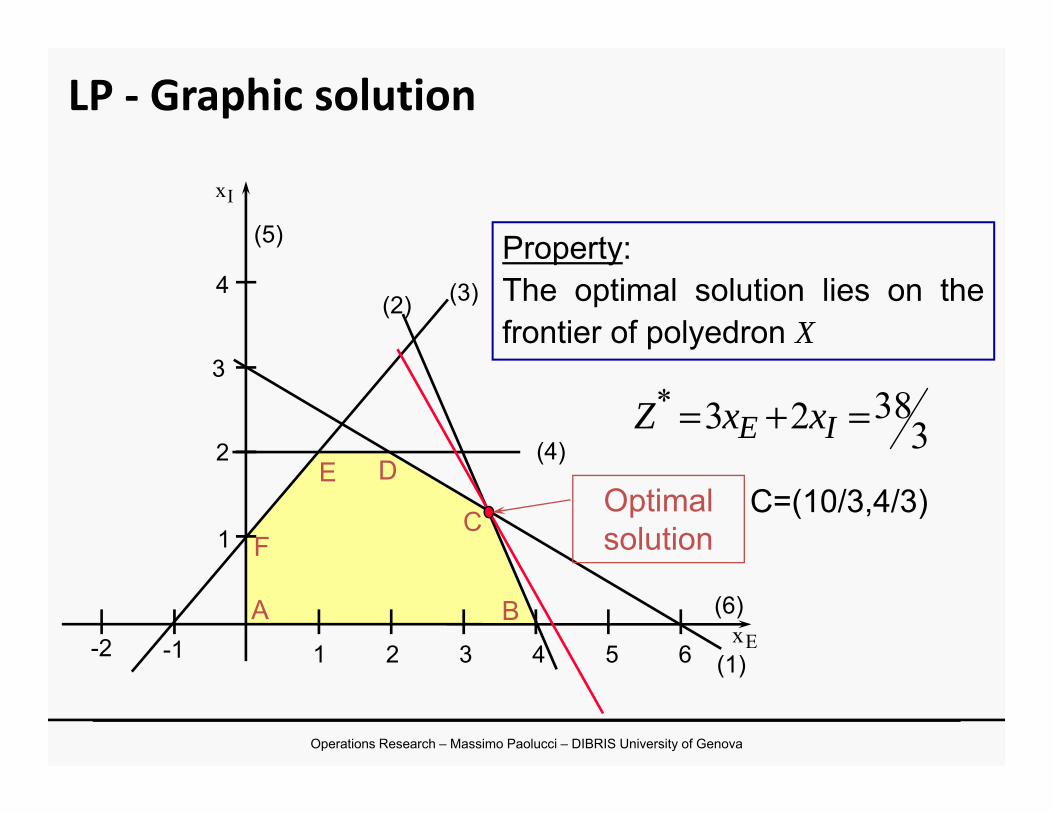
A
F
E D
B
CC=(10/3,4/3)Optimal
solution
33823* =+= IE xxZ
Property:The optimal solution lies on thefrontier of polyedron X
LP - Graphic solution
Operations Research – Massimo Paolucci – DIBRIS University of Genova
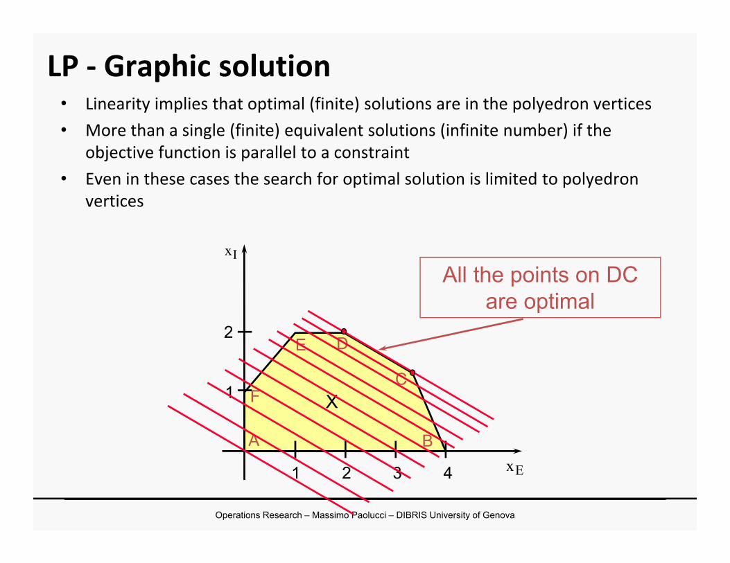
• Linearity implies that optimal (finite) solutions are in the polyedron vertices• More than a single (finite) equivalent solutions (infinite number) if the
objective function is parallel to a constraint• Even in these cases the search for optimal solution is limited to polyedron
vertices
1
2
F
E D
B
C
xE
xI
1 2 3 4
X
A
All the points on DC are optimal
LP - Graphic solution
Operations Research – Massimo Paolucci – DIBRIS University of Genova
• In the paint production problem it can be interesting to know how the raw materials (available resources) are used:– Is there any advantage from an increase of the resource availability?
– Is it possible to decrease the resource availability without changing the optimal objective value?
• Another interesting point is to analyse how the optimal solution would change if the selling prices change
LP – Graphic solution and post-optimality
Operations Research – Massimo Paolucci – DIBRIS University of Genova
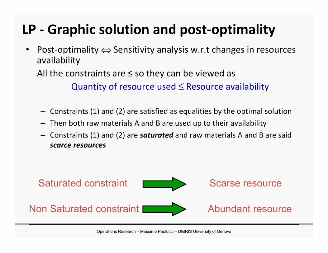
• Post-optimality ⇔ Sensitivity analysis w.r.t changes in resources availabilityAll the constraints are ≤ so they can be viewed as
Quantity of resource used ≤ Resource availability
– Constraints (1) and (2) are satisfied as equalities by the optimal solution– Then both raw materials A and B are used up to their availability– Constraints (1) and (2) are saturated and raw materials A and B are said
scarce resources
Saturated constraint Scarse resource
Non Saturated constraint Abundant resource
LP - Graphic solution and post-optimality
Operations Research – Massimo Paolucci – DIBRIS University of Genova
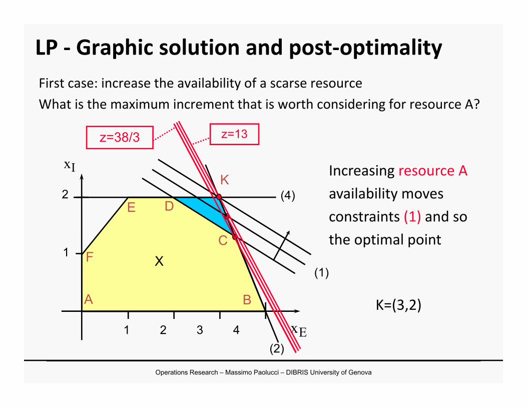
First case: increase the availability of a scarse resourceWhat is the maximum increment that is worth considering for resource A?
(1)1
2
A
F
E D
B
C
xE
xI
1 2 3 4
X
(2)
(4)K
z=38/3 z=13
Increasing resource Aavailability moves constraints (1) and so the optimal point
K=(3,2)
LP - Graphic solution and post-optimality
Operations Research – Massimo Paolucci – DIBRIS University of Genova
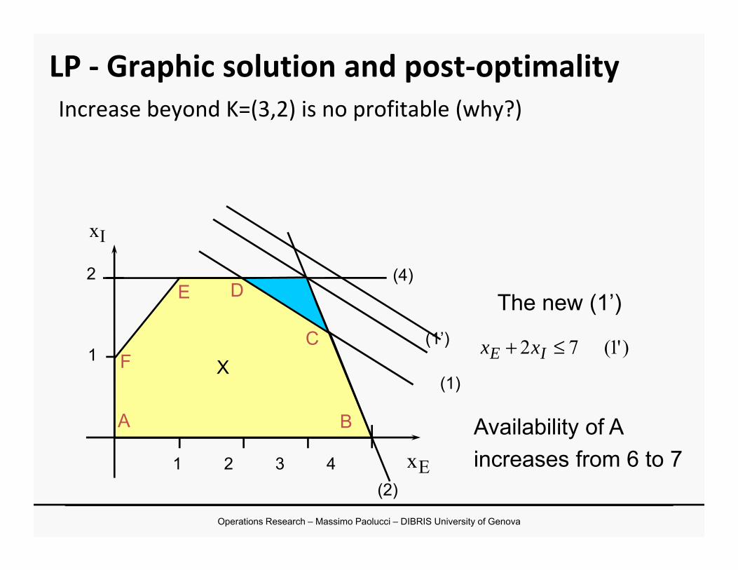
Increase beyond K=(3,2) is no profitable (why?)
(1)1
2
A
F
E D
B
C
xE
xI
1 2 3 4
X
(2)
(4)
Availability of A increases from 6 to 7
)'1(72 ≤+ IE xx
The new (1’)(1’)
LP - Graphic solution and post-optimality
Operations Research – Massimo Paolucci – DIBRIS University of Genova
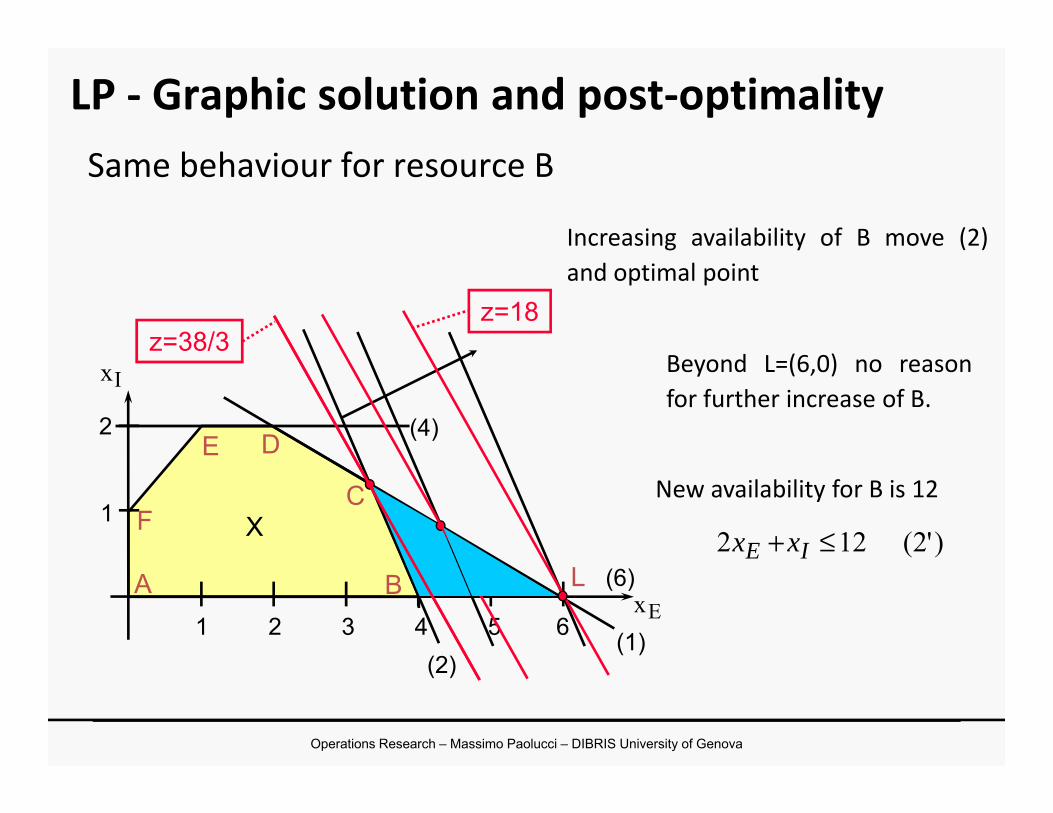
Same behaviour for resource B
1
2
A
F
E D
B
C
xE
xI
X
(2)
(4)
(1)1 2 3 4 5 6
(6)L
z=38/3z=18
Increasing availability of B move (2)and optimal point
Beyond L=(6,0) no reasonfor further increase of B.
New availability for B is 12
)'2(122 ≤+ IE xx
LP - Graphic solution and post-optimality
Operations Research – Massimo Paolucci – DIBRIS University of Genova
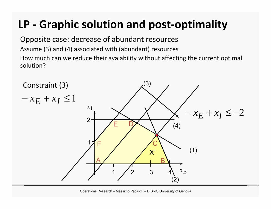
Opposite case: decrease of abundant resourcesAssume (3) and (4) associated with (abundant) resourcesHow much can we reduce their avalability without affecting the current optimal solution?
Constraint (3)
(4)
(2)
(1)
(3)
1
2
B
C
xE
xI
1 2 3 4
A
F
E D
X
A
F
E D
X’
1≤+− IE xx2−≤+− IE xx
LP - Graphic solution and post-optimality
Operations Research – Massimo Paolucci – DIBRIS University of Genova
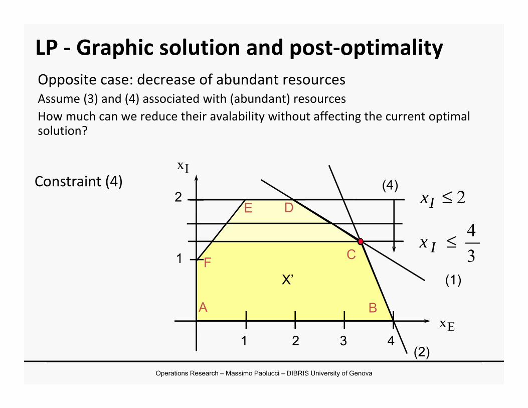
Opposite case: decrease of abundant resourcesAssume (3) and (4) associated with (abundant) resourcesHow much can we reduce their avalability without affecting the current optimal solution?
Constraint (4)
1
2
A
F
B
C
xE
xI
1 2 3 4
X
(2)
(4)
(1)
DE DE
X’
2≤Ix
34≤Ix
LP - Graphic solution and post-optimality
Operations Research – Massimo Paolucci – DIBRIS University of Genova
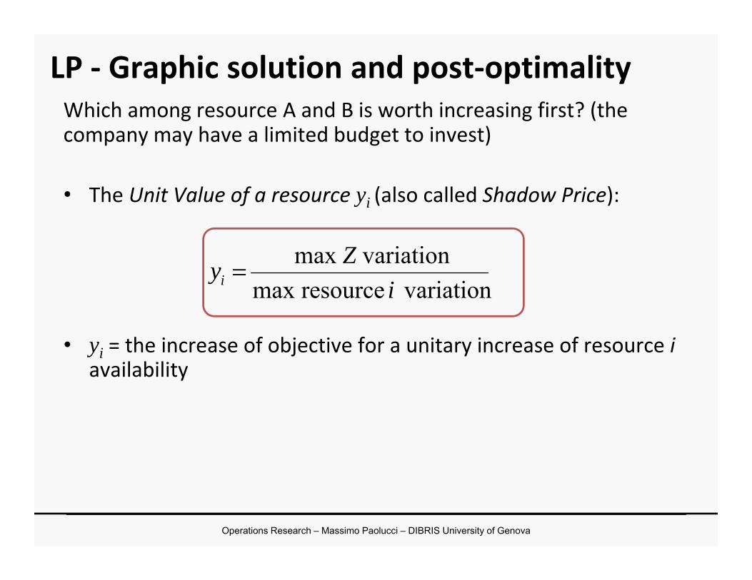
Which among resource A and B is worth increasing first? (the company may have a limited budget to invest)
• The Unit Value of a resource yi (also called Shadow Price):
• yi = the increase of objective for a unitary increase of resource iavailability
variation resourcemaxvariationmax
iZyi =
LP - Graphic solution and post-optimality
Operations Research – Massimo Paolucci – DIBRIS University of Genova
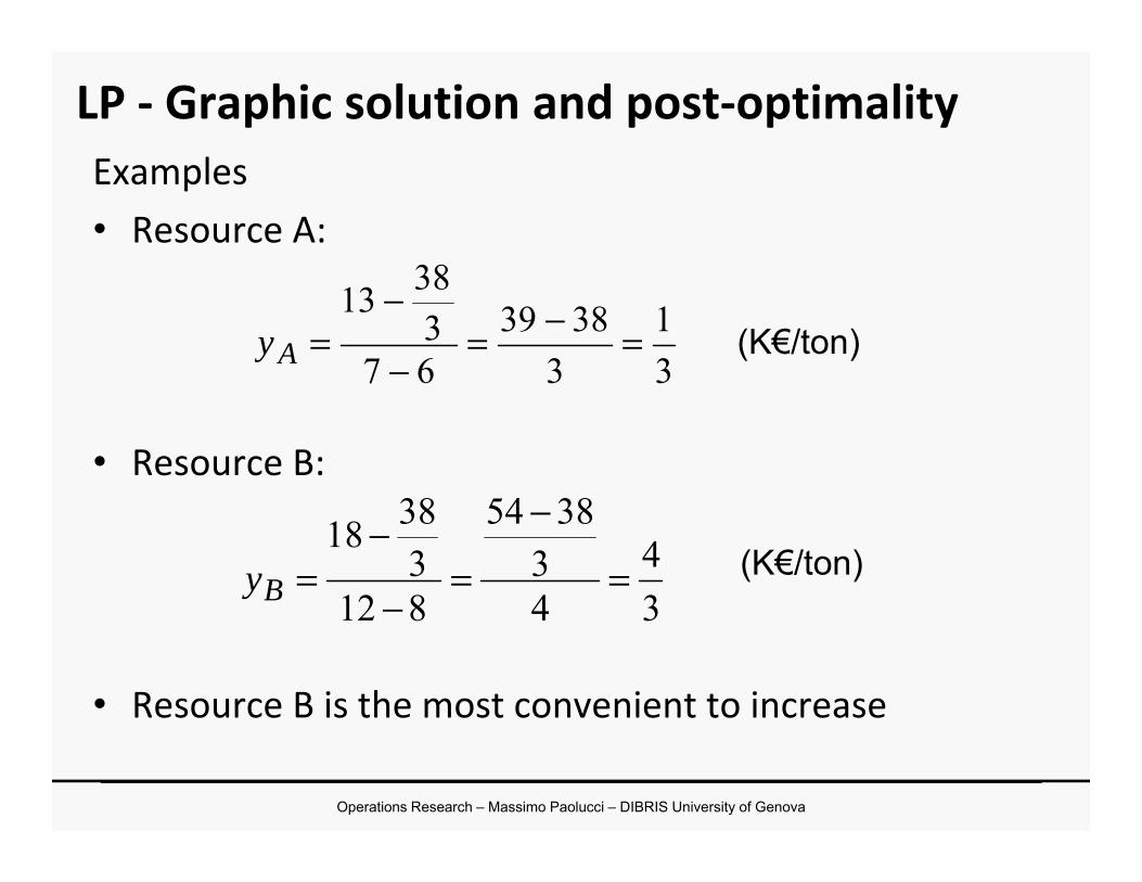
Examples• Resource A:
• Resource B:
• Resource B is the most convenient to increase
(K€/ton)31
33839
673
3813=−=
−
−=Ay
34
43
3854
8123
3818=
−
=−
−=By (K€/ton)
LP - Graphic solution and post-optimality
Operations Research – Massimo Paolucci – DIBRIS University of Genova
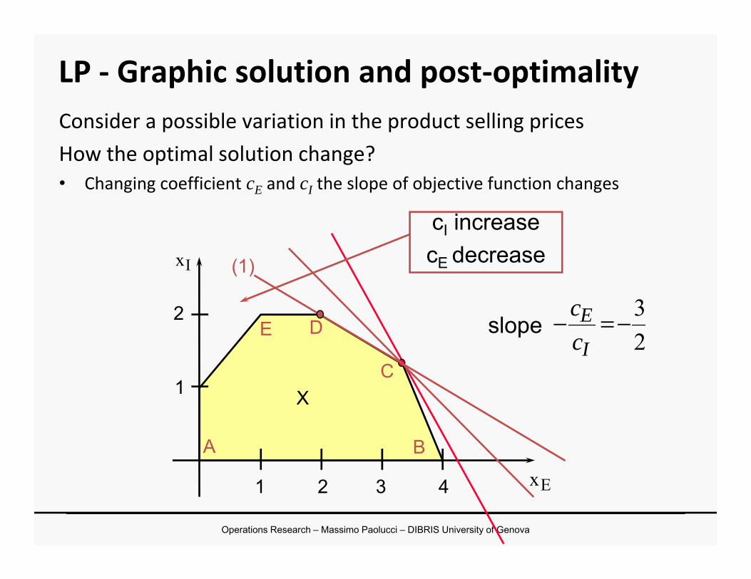
LP - Graphic solution and post-optimalityConsider a possible variation in the product selling pricesHow the optimal solution change? • Changing coefficient cE and cI the slope of objective function changes
F1
2
A
E D
B
C
xE
xI
1 2 3 4
X
cI increasecE decrease(1)
slope23−=−
I
Ecc
Operations Research – Massimo Paolucci – DIBRIS University of Genova
slope23−=−
I
Ecc
F1
2
A
E D
B
C
xE
xI
1 2 3 4
X
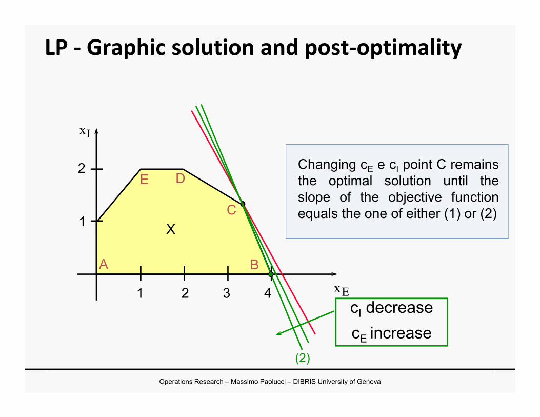
cI decreasecE increase
(2)
Changing cE e cI point C remainsthe optimal solution until theslope of the objective functionequals the one of either (1) or (2)
LP - Graphic solution and post-optimality
Operations Research – Massimo Paolucci – DIBRIS University of Genova
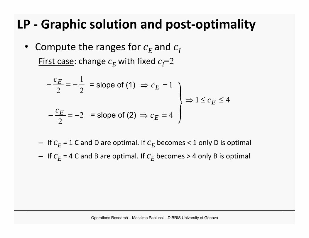
• Compute the ranges for cE and cIFirst case: change cE with fixed cI=2
– If cE = 1 C and D are optimal. If cE becomes < 1 only D is optimal
– If cE = 4 C and B are optimal. If cE becomes > 4 only B is optimal
21
2−=− Ec
= slope of (1) 1= Ec
= slope of (2)22
−=− Ec 4= Ec
41 ≤≤ Ec
LP - Graphic solution and post-optimality
Operations Research – Massimo Paolucci – DIBRIS University of Genova
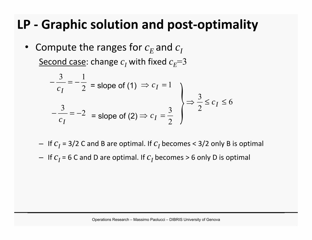
• Compute the ranges for cE and cISecond case: change cI with fixed cE=3
– If cI = 3/2 C and B are optimal. If cI becomes < 3/2 only B is optimal
– If cI = 6 C and D are optimal. If cI becomes > 6 only D is optimal
= slope of (1)
= slope of (2)
LP - Graphic solution and post-optimality
213 −=−
Ic
23 −=−Ic
1= Ic
23= Ic
623 ≤≤ Ic