WP/07/239

Operational Risk—The Sting is Still in the Tail but the Poison Depends on the Dose

Andreas A. Jobst

© 2007 International Monetary Fund WP/ IMF Working Paper Monetary and Capital Markets Department

Operational Risk—The Sting is Still in the Tail but the Poison Depends on the Dose

Prepared by Andreas A. Jobst

Authorized for distribution by Ceyla Pazarbasioglu

November 2007

Abstract

This Working Paper should not be reported as representing the views of the IMF. The views expressed in this Working Paper are those of the author(s) and do not necessarily represent those of the IMF or IMF policy. Working Papers describe research in progress by the author(s) and are published to elicit comments and to further debate.

This paper investigates the generalized parametric measurement methods of aggregate operational risk incompliance with the regulatory capital standards for operational risk in the New Basel Capital Accord (“Basel II”). Operational risk is commonly defined as the risk of loss resulting from inadequate or failed internal processes and information systems, from misconduct by people or from unforeseen external events. Ouranalysis informs an integrated assessment of the quantification of operational risk exposure and the consistency of current capital rules on operational risk based on generalized parametric estimation. JEL Classification Numbers: G10, G20, G21, G32, D81 Keywords: operational risk, risk management, financial regulation, Basel Committee, Basel II, New Basel

Capital Accord, extreme value theory, generalized extreme value (GEV) distribution, extremevalue theory (EVT), generalized Pareto distribution (GPD), peak-over-threshold (POT) method, g-and-h distribution, fat tail behavior, extreme tail behavior, Value-at-Risk (VaR), AdvancedMeasurement Approaches (AMA), risk measurement.

Author’s E-Mail Address: ajobst@imf.org

2

Contents Page

I. Introduction....................................................................................................................4

A. The Definition of Operational Risk, Operational Risk Measurement, and the Regulatory Framework for Operational Risk Framework For Operational

Risk Under the New Basel Capital Accord...........................................4 B. Literature Review .................................................................................................7 C. Objective...............................................................................................................8

II. The Use of EVT for Operational Risk Measurement in the Context of the New Basel

Capital Accord.........................................................................................................11 III. EVT and Alternative Approaches................................................................................14

D. The Limit Theorem of EVT the Relation Between GEV and GPD...................14 E. Definition and Parametric Specification of GEV ...............................................14 F. Definition and Parametric Specification of GPD................................................16 G. Definition and Parametric Estimation of the g-and-h Distribution ....................19

IV. Data Description ..........................................................................................................20

H. Data Generation: Simulation of a Quasi-Empirical Distribution .......................20 I. Aggregate Descriptive Statistics ........................................................................24

V. Estimation Procedure and Discussion..........................................................................25

J. Threshold Diagnostics: Slope of Mean Excess Function (MEF) and Stability of the Tail Index..............................................................................................26

K. Robustness of GPD Point Estimates to Threshold Choice.................................29 L. Backward Induction of the Optimal Threshold Choice .....................................32

VI. Conclusion ...................................................................................................................34 References................................................................................................................................38 Tables 1. Overview of Operational Risk Measures According to the Basel Committee on

Banking Supervision…..........................................................................................49 2. Aggregate Operational Risk Losses of U.S. Commercial Banks (Longitudinal)… ....50 3. Aggregate Operational Risk Losses of U.S. Commercial Banks (Cross-Sectional)…51 4. Descriptive Statistics of Simulated Daily Operational Risk Losses (Five-Year

Horizon).................................................................................................................52 5. Descriptive Statistics of Simulated Daily Operational Risk Losses (One-Year

Horizon).................................................................................................................53

3

6. Descriptives of Simulated Loss Series Based on the Aggregate Loss Statistics (2000–2004)… ......................................................................................................54

7. Descriptives of Quarterly Aggregates of Simulated Loss Series….............................55 8. Point Estimates of the Empirical, Normal and EVT-Based Distribution (Five-Year

Risk Horizon)….. ..................................................................................................57 9. Relative Deviation of Point Estimates of the Empirical, Normal and EVT-Based

Distribution (Five-Year Risk Horizon)..................................................................58 10. Point Estimates of the Empirical, Normal and EVT-Based Distribution (One-Year-

Risk Horizon)…. ...................................................................................................59 11. Estimated Parameter Values from the Numerical Evaluation of the Tail Behavior ....60 12. Summary Statistics of the Deviation of Point Estimates from the Actual Upper Tail

(Variable Threshold) Choice .................................................................................64 13. Summary Statistics of the Deviation of Point Estimates Around the Actual Upper Tail

Quantile (Variable Percentile)…...........................................................................66 14. Summary Statistics of Quantile (Point) Estimates of the EVT-Based

Distribution ….......................................................................................................71 Figures 1. Loss Distribution Approach (LDA) for AMA of Operational Risk ............................48 2. Upper Tail Graphs of Estimated Shape Parameter for a Continuous Threshold

Choice....................................................................................................................56 3. Threshold-Quantile Surface of Operational Risk Event... ...........................................61 4. Aggregate Sensitivity of Estimated Upper Tail to the Threshold Choice .. ................63 5. Aggregate Sensitivity of Individual Point Estimates to the Percentile Level of

Statistical Confidence ............................................................................................65 6. Single Point Estimate Graphs of GDP-Fitted Distribution (Variable Threshold) .......67 7. Relative Deviation of Point Estimates (Point Estimate Residuals) from the Actual

Quantile Level …. .................................................................................................68 8. Single Point Estimate Graphs of GPD-Fitted Distribution Threshold Upper Tail

Graphs....................................................................................................................69 9. Relative Deviation Of Point Estimates (Point Estimate Residuals) from Actual

Quantile Value .............................................................................................................70

4

Equation Chapter 1 Section 1

I. INTRODUCTION 1. After more than seven years in the making, the New Basel Capital Accord on global rules and standards of operation for internationally active banks has finally taken effect. At the end of 2006, the Basel Committee on Banking Supervision issued the final draft implementation guidelines for new international capital adequacy rules (International Convergence of Capital Measurement and Capital Standards or short “Basel II”) to enhance financial stability through the convergence of supervisory regulations governing bank capital (Basel Committee, 2004, 2005, and 2006b). The latest revision of the Basel Accord represents the second round of regulatory changes since the original Basel Accord of 1988. In a move away from rigid controls, the revised regulatory framework aligns minimum capital requirements closer to the actual friskiness of bank assets by allowing advanced risk measurement techniques. The new, more risk-sensitive capital standards are designed to improve the allocation of capital in the economy by more accurately measuring financial exposures to sources of risk other than market and credit risks.1 On the heels of prominent accounting scandals in the U.S. and greater complexity of financial intermediation, particularly operational risk and corporate governance have become salient elements of the new banking regulation. Against the background of new supervisory implementation guidelines of revised capital rules for operational risk in the U.S. (New Advanced Capital Adequacy Framework), which were published on February 28, 2007 (Federal Information & News Dispatch, 2007), this paper presents a quantitative modeling framework compliant with AMA risk measurement standards under the New Basel Capital Accord. Our generalized parametric estimation of operational risk of U.S. commercial banks ascertains the coherence of current capital rules and helps assess the merits of various private sector initiatives aimed at changing the proposed new regulatory standards for operational risk. A. The Definition of Operational Risk, Operational Risk Measurement, and the Regulatory

Framework for Operational Risk Under the New Basel Capital Accord 2. Operational risk has always existed as one of the core risks in the financial industry. However, over the recent past, the globalization and deregulation of financial markets, the growing complexity in the banking industry, large-scale mergers and acquisitions, increasing sophistication of financial products as well as greater use of outsourcing arrangements have raised the susceptibility of banking activities to operational risk. Although there is no agreed upon universal definition of operational risk, it is commonly defined as the risk of loss some adverse outcome, such as financial loss, resulting from acts undertaken (or neglected) in carrying

1 The revised version of the Basel Capital Accord rests fundamentally on three regulatory pillars: (i) “Minimum Capital Requirements” (Pillar 1), similar to the 1988 minimum capital requirements set forth in the original Basel Capital Accord, (ii) “Supervisory Review” (Pillar 2), which allows national supervisory authorities to select regulatory approaches that are deemed appropriate to the local financial structure, and (iii) “Market Discipline” (Pillar 3), which encourages transparent risk management practices.

5

out business activities, such as inadequate or failed internal processes and information systems, from misconduct by people (e.g., breaches in internal controls and fraud) or from external events (e.g., unforeseen catastrophes) (Basel Committee, 2004, 2005, and 2006b; Coleman and Cruz, 1999). 3. The measurement and regulation of operational risk is quite distinct from other types of banking risks. The diverse nature of operational risk from internal or external disruptions to business activities and the unpredictability of their overall financial impact complicate systematic and coherent measurement and regulation. Operational risk deals mainly with tail events rather than central projections or tendencies, reflecting aberrant rather than normal behavior and situations. Thus, the exposure to operational risk is less predictable and even harder to model. While some types of operational risks are measurable, such as fraud or system failure, others escape any measurement discipline due to their inherent characteristics and the absence of historical precedent. The typical loss profile from operational risk contains occasional extreme losses among frequent events of low loss severity (see Figure 1). Hence, banks categorize operational risk losses into expected losses (EL), which are absorbed by net profit, and unexpected losses (UL), which are covered by risk reserves through core capital and/or hedging. While banks should generate enough expected revenues to support a net margin after accounting for the expected component of operational risk from predictable internal failures, they also need to provision sufficient economic capital to cover the unexpected component or resort to insurance (Jobs, 2007a). 4. There are three major concepts of operational risk measurement: (I) the volume-based approach, which assumes that operational risk exposure is a function of the complexity of business activity, especially in cases when notoriously low margins (such as in transaction processing and payments-system related activities) magnify the impact of operational risk losses; (ii) the qualitative self-assessment of operational risk, which is predicated on subjective judgment and prescribes a comprehensive review of various types of errors in all aspects of bank processes with a view to evaluate the likelihood and severity of financial losses from internal failures and potential external shocks; and (iii) quantitative techniques, which have been developed by banks primarily for the purpose of assigning economic capital to operational risk exposures in compliance with regulatory capital requirements. The most prominent methods quantify operational risk by means of the joint and marginal distributions of the severity and the frequency of empirical and simulated losses in scenario testing. This approach caters to the concept of Value-at-Risk (VaR), which defines an extreme quantile as maximum limit on potential losses that are unlikely to be exceeded over a given time horizon (or holding period) at a certain probability (Mats, 2002 and 2003). 5. After the first industry-wide survey on existing operational risk management (ORM) standards in 1998 exposed an ambivalent definition of operational risk across banks, regulatory efforts by the Basel Committee have contributed in large parts to the evolution of quantitative

6

methods as a distinct discipline of operational risk measurement.2 The new capital rules stipulated by the Operational Risk Subgroup (AIGOR) of the Basel Committee Accord Implementation Group define three different quantitative measurement approaches for operational risk (see Table 1) in a continuum of increasing sophistication and risk sensitivity based on eight business lines (Bless) and seven event types (Est.) as units of measure3 for operational risk reporting (Basel Committee, 2001a, 2001b, 2002, 2003a and 2003b). The Basic Indicator Approach (BIA) and the Standardized Approach (TSA) under the new capital rules assume a fixed percentage of gross income as a volume-based metric of operational risk, whereas eligible Advanced Measurement Approaches (AMA) define a capital measure of operational risk that is explicitly and systematically more sensitive to the varying risk profiles of individual banks. AMA banks use internal risk measurement systems and rely on self-assessment via scenario analysis to calculate regulatory capital that cover their total operation risk exposure (both EL and UL) over a one-year holding period at a 99.9 percent statistical confidence level.4 To this end, the Loss Distribution Approach (LDA) has emerged as the most common form of measuring operational risk based on an annual distribution of the number and the total loss amount of operational risk events and an aggregate loss distribution that combines both frequency and loss severity. The two alternative approaches under the proposed regulatory regime, BIA and TSA, define deterministic standards of regulatory capital measurement. BIA requires banks to provision a fixed percentage (15 percent) of their average gross income over the previous three years for operational risk losses, whereas TSA5 sets regulatory capital to at least the three-year average of the summation of different regulatory capital charges (as a percentages of gross income) across Bless in each year (Jobs, 2007b).6

2 The Consultative Document on Operational Risk (Basel Committee, 2001c), the Working Paper on the Regulatory Treatment of Operational Risk (Basel Committee, 2001b), the Sound Practices for the Management and Supervision of Operational Risk (Basel Committee, 2001a, 2002 and 2003b) and the new guidelines on the International Convergence of Capital Measurement and Capital Standards (Basel Committee, 2004, 2005 and 2006b) define the regulatory framework for operational risk. 3 A unit of measure represents the level at which a bank’s operational risk quantification system generates a separate distribution of potential operational risk losses (Seivold et al., 2006). A unit of measure could be a business line (BL), an event type (ET) category, or both. The Basel Committee specifies eight BLs and seven ETs for operational risk reporting. 4 The most recent report by the Basel Committee (2006a) on the Observed Range of Practice in Key Elements of Advanced Measurement Approaches (AMA) illustrates how far international banks have developed their internal operational risk management (ORM) processes in line with the qualitative and quantitative criteria of AMA. 5 At national supervisory discretion, a bank can be permitted to apply the Alternative Standardized Approach (ASA) if it provides an improved basis for the calculation of minimum capital requirements by, for instance, avoiding double counting of risks (Basel Committee, 2004 and 2005). 6 See also Basel Committee (2003a, 2001b, and 1998). Also note that in both approaches periods in which gross income is negative or zero are excluded.

7

B. Literature Review 6. The historical loss experience serves as a prime indicator of the amount of reserves banks need to hold to cover the financial impact of operational risk events. However, the apparent paucity of actual loss data, the inconsistent recording of operational risk events, and the intricate characteristics of operational risk complicate the consistent and reliable measurement of operational risk. Given these empirical constraints on supervisory guidelines, researchers at regulatory authorities, most notably at the Federal Reserve Bank of Boston (Dutta and Perry, 2006; de Fontnouvelle et al., 2004) and the Basel Committee (Moscadelli, 2004) have examined how data limitations impinge on the calculation of operational risk estimates in a bid to identify general statistical patterns of operational risk across banking systems. At the same time, academics and industry professionals have devised quantitative methods to redress the apparent lack of a comprehensive and cohesive operational risk measurement. Several empirical papers have explored ways to measure operational risk exposure at a level of accuracy and precision comparable to other sources of risk (Chernobai and Rachev, 2006; Degen et al., 2006; Makarov, 2006; Mignola and Ugoccioni, 2006 and 2005; Nešlehová et al., 2006; Grody et al, 2005; Alexander, 2003; Coleman and Cruz, 1999; Cruz et al., 1998). 7. Despite the popularity of quantitative methods of operational risk measurement, these approaches frequently ignore the quality of potentially offsetting risk control procedures and qualitative criteria that elude objective measurement concepts. Several theoretical models center on the economic incentives for sustainable ORM. Leippold and Vanini (2003) consider ORM as a means of optimizing the profitability of an institution along its value chain, while Banerjee and Banipal (2005) and Crouhy et al. (2004) model the effect of an operational risk event on the utility of both depositors and shareholders of banks as an insurance problem. Crouhy et al. (2004) show that lower regulatory capital due to the partial recognition of the risk-mitigating impact of insurance would make some banks better off if they self-insured their operational risk depending on their capital structure, operational risk loss, expected return on assets and the risk-neutral probability of an operational risk event. Banerjee and Banipal (2005) suggest that as the volume of banking business increases, it is optimal to allow bank management to choose their own level of insurance and regulatory capital in response to perceived operational risk exposure, whereas a blanket regulation on bank exposures can be welfare reducing. 8. Our paper fits seamlessly into existing empirical and theoretical research on operational risk as an extension to the parametric specification of tail convergence of simulated loss data in Mignola and Ugoccioni (2005). The main objective of this paper is the optimization of generalized parametric distributions (generalized extreme value distribution (GEV) and generalized Pareto distribution (GPD)) as the most commonly used statistical techniques for the measurement of operational risk exposure as extreme loss under extreme value theory (EVT). EVT is often applied as risk measurement panacea of high-impact, low-probability exposures due to the tractability and natural simplicity of order statistics—in many instances, regrettably, without consideration of inherent parameter instability of estimated asymptotic tail shape at extreme quantiles. We acknowledge this contingency by way of a detailed investigation of the contemporaneous effects of parameterization and desired statistical power on risk estimates of

8

simulated loss profiles. Our measurement approach proffers a coherent threshold diagnostic and model specification for stable and robust capital estimates consistent with a fair value-based insurance premium of operational risk presented by Banerjee and Banipal (2005). The consideration of gross income as exposure factor also allows us to evaluate the coherence of the present regulatory framework for a loss distribution independent of uniform capital charges under standardized approaches to operational risk (Mignola and Ugoccioni, 2006) and extend beyond a mere discussion of an appropriate modeling technique (de Fontnouvelle et al, 2004). 9. Previous studies suggest that the asymptotic tail behavior of excess distributions could exhibit weak convergence to GPD at high empirical quantiles due to the second order behavior of a slowly varying loss severity function.7 Degen et al. (2006) tender the g-and-h distribution as a suitable candidate for the loss density function of operational risk. Therefore, we examine the ability of the g-and-h distribution (which approximates even a wider variety of distributions than GEV and GPD) to accommodate the loss severity of different banks à la Dutta and Perry (2006), who focus on the appropriate measurement of operational risk rather than the assessment of whether certain techniques are suitable for modeling a distinct loss profile of a particular entity.

C. Objective 10. In this paper, we investigate the concept of EVT and the g-and-h distribution as measurement methods of operational risk in compliance with the regulatory capital standards of the New Basel Capital Accord. Both methods establish an analytical framework to assess the parametric fit of a limiting distribution to a sequence of i.i.d. normalized extremes of operational risk losses.8 The general utility of this exercise lies in the estimation of UL from a generic loss profile simulated from the aggregate statistics of the historical loss experience of U.S. commercial banks that participated in a recent operational risk survey conducted by U.S. banking supervisors. 11. Our approach helps ascertain the economic implications associated with the quantitative characteristics of heterogeneous operational risk events and informs a more judicious metric of loss distributions with excess elongation. In this way, we derive more reasonable conclusions regarding the most reliable estimation method for the optimal parametric specification of the limiting behavior of operational risk losses at a given percentile level (Basel Committee, 2003a). In particular, we can quantify the potential impact of operational risk on the income performance of a selected set of banks at any given point in time if they were subject to the aggregate historical loss experience of the largest U.S. commercial banks over the last five years.

7 Degen et al. (2006) find that EVT methodologies would overstate point estimates of extreme quantiles of loss distributions with very heavy tails if the g-and-h distribution would provide better overall fit for kurtosis parameter

0h = (see section G). 8 These extremes are considered to be drawn from a sample of dependent random variables.

9

12. As the most widely established generalized parametric distributions under EVT,9 we fit the GEV and GPD to the empirical quantile function of operational risk losses based on a “full-data” approach, by which all of the available loss data are utilized at an (aggregate) enterprise level.10 The latter form of EVT benefits from the versatility of being an exceedance function, which specifies the residual risk in the upper tail of GEV-distributed extreme losses beyond a threshold value that is sufficiently high to support linear conditional mean excess. As an alternative generalized parametric specification, we apply the g-and-h distribution, which also relies on the order statistic of extremes, but models heavy-tailed behavior by transforming a standard normal variable. Both methods are appealing statistical concepts, because they deliver closed form solutions for the probability density of operational risk exposures at very high confidence levels if certain assumptions about the underlying data hold. 13. Since our modeling approach concurs with the quantitative criteria of operational risk estimates under AMA, we also evaluate the adequacy and consistency of capital requirements for operational risk and the soundness of accepted measurement standards under the current regulatory framework set forth in the New Basel Capital Accord. As part of our econometric exercise, we can assess the sensitivity of capital charges for UL (compliant with AMA) to (internal) assumptions influencing the quantitative modeling of economic capital. Similarly, we evaluate the suitability of external, volume-based measurement standards (i.e., BIA)11 to establish an accurate level of the regulatory capital to cover actual operational risk exposure. Based on accurate and stable analytical loss estimates, we compare AMA results to principles and practices of standardized measurement methodologies in view of establishing empirically valid levels of regulatory capital coverage for operational risk. Since we simulate aggregate losses from a generic loss severity function based on descriptive statistics of the 2004 Loss Data Collection Exercise (LDCE), we cannot, however, investigate the robustness of internal measurement models to accommodate different loss distributions across banks (i.e., internally consistent cross-sectional differences).

9 Our modeling choice coincides with the standard operational risk measurement used by AMA banks. In anticipation of a changing regulatory regime, the development of internal risk measurement models has led to the industry consensus that EVT could be applied to satisfy the Basel quantitative standards for modeling operational risk (McConnell, 2006). According to Dutta and Perry (2006) five out of seven institutions in their analysis of U.S. commercial banks with comprehensive internal loss data reported using some variant of EVT in the 2004 Loss Data Collection Exercise (LDCE), which was jointly organized by U.S. banking regulatory agencies. 10 Measuring operational risk exposure at the enterprise level is advantageous, because more loss data is available for the parametric estimation; however, this comes at the expense of similar losses being grouped together. 11 Since we do not distinguish operational risk losses as to their specific cause and nature (i.e., different BLs and ETs), our results do not permit us to assess, in more detail, the actual applicability of setting regulatory capital according to TSA or ASA. The suitability of the BIA can be tested by either contrasting the analytical loss estimate at the 99.9th percentile (adjusted by gross income) and a standard capital charge of 15 percent of average gross income over three years or estimating the level of statistical confidence at which the analytical point estimate concurs with a capital charge of 15 percent.

10

14. We find that a standard volume-based metric of unexpected operational risk is exceedingly simplistic and belies substantial heterogeneity of relative operational risk losses across banks. Our simulation results suggest that cumulative operational risk losses arising from consolidated banking activities hardly surpass 2 percent of quarterly reported gross income and clearly undershoot a fixed regulatory benchmark in the range between 12 and 18 percent.12

Therefore, aggregate measures of operational risk with no (or limited) discriminatory use of idiosyncratic adjustment in volume-based risk estimates adjustment seem to be poor indicators of regulatory capital if the actual operational risk losses exposure deviates from generic assumptions about the potential impact of operational risk implied by the standardized regulatory provisions. 15. We find that internal risk models based on the generalized parametric fit of empirical losses substantiate close analytical risk estimates of UL. The quantitative self-assessment of operational risk in line with AMA yields a more realistic measure of operational risk exposure than standardized approaches and implies substantial capital savings of up to almost 97 percent. However, the regulatory 99.9th percentile restricts estimation methods to measurement techniques, whose risk estimates are notoriously sensitive to the chosen calibration method, the threshold choice, and the empirical loss profile of heterogeneous banking activities. Since the scarcity of historical loss data defies back-testing, any estimation technique of residual risk at high percentile levels is therefore invariably beset by considerable parameter risk. The most expedient and stable parametric estimation of asymptotic tail behavior under these conditions necessitates the designation of extremes beyond a loss threshold close to the desired level of statistical confidence (“in-sample estimation”)—subject to the general sensitivity of point estimates. Based on our simulated sample of operational risk losses, reflecting the average historical loss experience of U.S. commercial banks, at least 1.5 percent of all operational risk events would need to be considered extremes by historical standards in order to support reliable point estimates at a statistical confidence level of no higher than 99.0 percent. This result makes the current regulatory standards appear overly stringent and impractical. Estimation uncertainty increases significantly when the level of statistical confidence exceeds 99.7 percent or fewer than 0.5 percent of all loss events can be classified as exceedances for parametric upper tail fit. At the same time, a marginal reduction of the percentile level by 0.2 percentage points from 99.9 percent to 99.7 percent reduces both UL and the optimal threshold at lower estimation uncertainty, requiring a far smaller sample size of essential loss data. For the parametric estimation under GPD, the Moment and MLE estimation algorithms generate the most accurate point estimates for the approximation of asymptotic tail behavior, regardless of varying tail shape properties of different loss profiles. The g-and-h offers a more consistent upper tail fit than GPD, and generates more accurate and realistic point estimates only beyond the critical 99.9th percentile level.

12 Although point estimates would increase based on a more fine-tuned, business activity-specific volume adjustment, the variation of relative loss severity across banks remains.

11

16. The paper is structured as follows. After a brief description of the data generation process and conventional statistical diagnostics in the next section, we define the GEV, GPD, and the g-and-h distributions as the most prominent methods to model limiting distributions with extreme tail behavior. We then establish the statistical foundation for the application of the selected generalized parametric distributions to simulated extreme losses from operational risk. Since we are particularly interested in EVT, we review salient elements of the tail convergence of a sequence of i.i.d. normalized maxima to GEV and the GPD-based approximation of attendant residual risk beyond a specific threshold via the Peak-over-Threshold (POT) method. We complete comprehensive threshold diagnostics associated with the application of GPD as estimation method for observed asymptotic tail behavior of the empirical distribution of operational risk losses (e.g., the slope of the conditional mean excess function and the stability of GPD tail parameter estimates). In addition, we introduce the g-and-h distribution as alternative parametric approach to examine the alleged tendency of EVT approaches to overstate point estimates at high percentile levels. In the third section, we derive analytical (in- and out-of-sample) point estimates of unexpected operational risk (adjusted by Tier 1 capital, gross income, total assets) for four sample banks at different percentile levels in accordance with the internal model-based approach of operational risk measurement under the New Basel Capital Accord. Subsequently, we discuss our findings vis-à-vis existing regulatory capital rules and examine how the level and stability of point estimates varies by estimation method. 17. Given the significant estimation uncertainty associated with the inherent sensitivity of GPD-based risk estimates to parameter stability, the linearity of mean excess, and the type of estimation procedure, we inspect the robustness of point estimates to the threshold choice and the stability of the goodness of upper tail fit over a continuous percentile range for different estimation methods (Moment, Maximum Likelihood, Pickands, Drees-Pickands, and Hill). We introduce the concept of a “threshold-quantile surface” (and its simplification in the form of “point estimate graphs” and “single threshold upper tail graphs”) as an integrated analytical framework to illustrate the model sensitivity of point estimates of operational risk losses to the chosen estimation method and parameter input for any combination of threshold choice and level of statistical confidence. The fourth section concludes the paper and provides recommendations for efficient operational risk measurement on the condition of existing regulatory parameters.

II. THE USE OF EVT FOR OPERATIONAL RISK MEASUREMENT IN THE CONTEXT OF THE NEW BASEL CAPITAL ACCORD

18. While EL attracts regulatory capital, exposures to low frequency but high-impact operational risk events underpinning estimates of UL require economic capital coverage. If we define the distribution of operational risk losses as an intensity process of time t (see Figure 1), the expected conditional probability ( ) ( ) ( ) ( ) ( ) 0EL T t E P T P t P T P t⎡ ⎤− = − − <⎣ ⎦ specifies the

average exposure over time horizon T, while the probability ( ) ( ) ( )UL T t P T t EL T tα− = − − − captures the incidence of losses higher than EL—but smaller than tail cut-off ( ) ( )E P T P tα −⎡ ⎤⎣ ⎦—

beyond which any residual or extreme loss (“tail risk”) occurs at a probability of α or less. This

12

definition of UL concurs with VaR, which prescribes a probabilistic bound of maximum loss over a defined period of time for a given aggregate loss distribution. Since AMA under the New Basel Capital Accord requires internal measurement methods of regulatory capital to cover UL13 over a one-year holding period at the 99.9 percent confidence level, VaR would allow the direct estimation of capital charges. However, heavy-tailed operational risk losses defy conventional statistical inference about loss severity as a central projection in conventional VaR when all data points of the empirical loss distribution are used to estimate maximum loss and more central (i.e., more frequent) observations (and not extremes) are fitted to high quantiles. 19. EVT can redress these shortcomings by defining the limiting behavior of empirical losses based on precise knowledge of extremely asymptotic (upper tail) behavior. Since this information helps compute more tail-sensitive VaR-based point estimates, integrating EVT into the VaR methodology can enhance operational risk estimates at extreme quantiles. Thus, the development of internal risk measurement models has spawned extreme value VaR (EVT-VaR) as a suitable and expedient methodology for calculating risk-based capital charges for operational risk under the New Basel Capital Accord. In this regard, the Loss Distribution Approach (LDA) measures operational risk as the aggregate exposure resulting from a fat-tailed probability function of loss severity compounded by the frequency of operational risk events over a certain period of time. 20. Despite the tractability of using order statistics for the specification of asymptotic tail behavior, the basic structure of EVT cannot, however, be applied readily to any VaR analysis without discriminate and conscientious treatment of unstable out-of-sample parameter estimates caused by second order effects of a slowly converging distribution of extremes. For EVT to be feasible for the parametric specification of a limiting distribution of operational risk losses, we need to determine (I) whether GEV of normalized random i.i.d. maxima correctly identifies the asymptotic tail convergence of designated extremes, and if so, (ii) whether fitting GPD as exceedance function to the order statistics of these observations (as conditional mean excess over a sufficiently high threshold value approaching infinity) substantiates a reliable, non-degenerate limit law that satisfies the external types theorem of GEV. The calibration of the g-and-h distribution—as an alternative approach to modeling the asymptotic tail behavior based on order statistics of extremes—does not entail estimation uncertainty from a discrete threshold choice as EVT. That said, the quality of the quantile-based estimation of this generalized parametric distribution hinges on the specification of the selected number and the spacing of percentiles in the upper tail (contingent on the correlation between the order statistics of extreme observations and their quantile values), whose effect on the parameterization of higher moments implies estimation risk.

13 Recent regulatory considerations of AMA also include a newsletter on The Treatment of Expected Losses by Banks Using the AMA under the Basel II Framework (2005) recently issued by AIGOR.

13

21. We derive risk estimates of aggregate operational risk within a “full data” approach by restricting our analysis to the univariate case. In keeping with the normative assumption of absent correlation between operational loss events, we rule out joint patterns of extreme behavior of two or more Bless or Est.. Note that the aggregation of i.i.d. random extremes (Longin, 2000) is not tantamount to the joint distribution of marginal extremes (Embrechts, 2000; Embrechts et al., 2003, 2001a, and 2001b) in absence of a principled standard definition of order in a vectorial space. Hence, the extension of EVT-VaR to the multivariate case of extreme observations would be inconclusive. Nonetheless, some methods have been proposed to estimate multivariate distributions of normalized maxima as n-dimensional asset vectors of portfolios, where parametric (Stephenson, 2002) or non-parametric (Pickands, 1981; Poon et al., 2003) models are used to infer the dependence structure between two or more marginal extreme value distributions.14

14 The multivariate extreme value distribution can be written as

( ) ( ) ( ){ }= = == − ∑ ∑ ∑11 1 1

exp , ...,n n n

i i n ii i iG x y A y y y y for ( )= 1 , ..., nx x x , where the ith univariate marginal

distribution ( ) ( )( ) ξξ μ σ

−= = + −

11 i

i i i i i iy y x x is generalized extreme value, with ( )ξ μ σ+ − >1 0i i ix , scale

parameter σ > 0i , location parameter μi , and shape parameter ξi . If ξ = 0i (Gumbel distribution), then iy is

defined by continuity. The dependence function ( ).A is defined on simplex { }1: 1

nnn ii

S ω ω+ == ∈ =∑R with

( ) ( )ω ω ω≤ ≤ ≤10 max , ..., 1n A for all ( )ω ω ω= 1 , ..., n . It is a convex function on [ ]0,1 with ( ) ( )= =0 1 1A A and

( ) ( )ω ω ω≤ − ≤ ≤0 max ,1 1A for all ω≤ ≤0 1 , i.e., the upper and lower limits of ( ).A are obtained under complete dependence and mutual independence respectively.

14

III. EVT AND ALTERNATIVE APPROACHES

D. The Limit Theorem of EVT the Relation Between GEV and GPD 22. We define EVT as a general statistical concept of deriving a limit law for sample maxima.15 GEV and GPD are the most prominent parametric methods for the statistical estimation of the limiting behavior of extreme observations under EVT. While the former models the asymptotic tail behavior of the order statistics of normalized maxima (or minima), the latter measures the residual risk of these extremes beyond a designated threshold as the conditional distribution of mean excess. The Pickands-Balkema-de Haan limit theorem (Balkema and de Haan, 1974; Pickands, 1975) postulates that GPD is the only non-degenerate limit law of observations in excess of a sufficiently high threshold, whose distribution satisfies the external types theorem (or Fisher-Tippett (1928) theorem).16 As a basic concept, fitting GPD to the distribution of i.i.d. random variables at very high quantiles approximates the asymptotic tail behavior of extreme observations under GEV as the threshold approaches the endpoint of the variable of interest, where only a few or no observations are available (Vandewalle et al., 2004).17,18

E. Definition and Parametric Specification of GEV 23. Let ( )1max ,..., nY X X= be the sample maximum (or minimum) of a sequence of i.i.d. random variables { }1 , ..., nX X with common c.d.f. F, density f, and ascending kth order statistics

,1 ,...n n nX X≤ ≤ in a set of n observations. GEV prescribes that there exists a choice of normalizing

constants 0na > and nb , such that the probability of a n-sequence of maxima ( )n nY b a− converges to [ ] ( ) ( )( ) ( ) ( )lim Pr

ntn n n n nn

F x Y b a y F a y b G x→∞

⎡ ⎤= − ≤ = + →⎣ ⎦ (1)

as n →∞ and x ∈R . If [ ] ( ) ( )n na x b

nF x G x+ ≈ , normalized maxima (or minima) are considered to

fall only within the maximum domain of attraction (MDA) of ( )G x , or ( )F D Gξ∈ . The three

distinct sub-classes of limiting distributions for external behavior (Gumbel, Fréchet or negative Weibull) are combined into the GEV probability density function

15 See Vandewalle et al. (2004), Stephenson (2002), and Coles et al. (1999) for additional information on the definition of EVT. 16 See also Gnedenko (1943). 17 For further references on the application of EVT in the estimation of heavy tailed financial returns and market risk see also Leadbetter et al. (1983), Leadbetter and Nandagoplan (1989), Mills (1995), Longin (1996), Resnik (1992), Embrechts et al. (1997), Danielsson and de Vries (1997a and 1997b), Resnik (1998), Diebold et al. (1998), Adler et al. (1998), McNeil and Frey (1999), McNeil (1999), Embrechts et al. (2002 and 1999), Longin (2000), Bermudez et al (2001), Longin and Solnik (2001), and Lucas et al (2002). 18 See Resnick (1992) for a formal proof of the theorem. See also Resnick (1998) and Gnedenko (1943).

15

( )( )( )( ) ( )( )( )( )( ) R

1

, ,

exp 1 1 0, 0

exp exp , 0,

x xG x

x x

ξ

ξ μ σ

ξ μ σ ξ μ σ ξ

μ σ ξ

−⎧ − + − + − > ≠⎪= ⎨⎪ − − − ∈ =⎩

, (2)

or briefly

( ) ( )( )( )1exp 1G x x

ξξ μ σ

−

+= − + − , (3)

for ( )max ,0h h+ = , after adjustment of (real) scale parameter 0σ > , (real) location parameter μ and the re-parameterization of the “tail index” 1α ξ= with shape parameter ξ , which indicates the velocity of asymptotic tail decay of a given limit distribution (“tail thickness”).19 The smaller the absolute value of the tail index (or the higher the shape parameter), the larger the weight of the tail and the slower the speed at which the tail approaches its peak on the x-axis at a y-value of 0 (asymptotic tail behavior).20

24. We estimate the parameters of GEV under two different assumptions. The distribution of normalized maxima of a given fat-tailed series either (i) converges perfectly to GEV or (ii) belongs to the MDA of GEV. In the first case, the location, scale and shape parameters are estimated concurrently by means numerical iteration in order to derive the point estimate.

( ) ( )( )ˆ

1ˆ ˆ ˆ, ,

ˆˆ ˆˆ ln 1px G p pξ

ξ μ σμ σ ξ

−− ⎛ ⎞= = + − −⎜ ⎟⎝ ⎠

, (4)

25. If the common distribution of observations satisfies ( )F D Gξ∈ only, then

( ) ( )lim lnn nnF x G xξσ μ

→∞+ = − , the GEV parameters are estimated semi-parametrically based on

( ) ( )1F x x L xξ−= for 0λ > and ( ) ( )( )lim 1x

L x L xλ→∞

= (Bensalah, 2000). For x →∞ and threshold

n nt xσ μ= + , [ ] ( ) ( ) ( )( )ˆ1

ˆ ˆ ˆ, ,ˆ ˆ ˆln 1

n n

tn nnF x G x x

ξ

ξ μ σξ μ σ

−≈ − = + − yields the approximative point

estimate 19 In the specification of GEV, the Gumbel type is defined by continuity as a single point in the continuous parameter space, i.e., the Gumbel type is essentially ignored in the process of fitting GEV. As we will see later on in the case of GPD, the same logic applies to the exponential distribution (Cohen, 1982a and 1982b). However, if we extrapolate asymptotic tail behavior into unobserved extremes, the Gumbel limit provides a better approximation the further into the tail the extrapolation is made. Stephenson and Tawn (2004) overcome the problem of selecting the extremal type prior to fitting GEV by introducing reversible jump Markov Chain Monte Carlo (MCMC) techniques as inference scheme that allows dimension switching between GEV (GPD) and the Gumbel (exponential) sub-model in order to assign greater possibility of Gumbel-type tail behavior within GEV (GPD). See also Kotz and Nadarajah (2000) for an authoritative overview of extreme value distributions. 20 The shape parameter ξ indicates highest bounded moment for the distribution, e.g. if 1 2ξ = , the first moment (mean) and the second moment (variance) exist, but higher moments have a infinite value. A positive shape parameter also implies that the moments of order 1n ξ≥ are unbounded.

16

( ) ( )( )ˆ

1ˆ ˆ ˆ, ,

ˆˆ ˆˆ ln 1 1n n

p n nx G p n pξ

ξ μ σμ σ ξ

−− ⎛ ⎞= − = + − −⎜ ⎟⎝ ⎠

. (5)

26. If the number of empirical observations of extremes is insufficient, we define a threshold t equal to the order statistic ,n kX of k exceedances in a series of n observations. Dividing

( ) ( )1ˆ ˆ ˆ 1p p pF x x L x pξ−= = − (see above) by ( ) ( )1, , ,n k n k n kF X X L X k nξ−= = yields the out-of-sample

point estimate of quantile

( )( )ˆ

,ˆ 1p n kx X n k p ξ−= − , (6)

where kp Xx >ˆ and ( ) ( )knp XLxL ,ˆ ≈ .21

F. Definition and Parametric Specification of GPD Definition 27. The parametric estimation of extreme value type tail behavior under GPD requires a threshold selection that guarantees asymptotic convergence to GEV. GPD approximates GEV according to the Pickands-Balkema-de Haan limit theorem only if the sample mean excess is positive linear and satisfies the Fisher-Tippett theorem. It is commonly specified as conditional mean excess distribution [ ] ( ) ( ) ( )Pr PrtF x X t x X t Y y X t= − ≤ > ≡ ≥ > of an ordered sequence of

exceedance values ( )1max ,..., nY X X= from i.i.d. random variables, which measures the residual risk beyond threshold ∞→t (Reiss and Thomas, 1997). GPD with threshold t →∞ represents the (only) continuous approximation of GEV (Castillo and Hadi, 1997) [ ] ( )( ) [ ] ( ) ( )( ), 1 log 1n na t b t

n nF a t s b W x G s tξ β ξ ξ+ + + → = + + , (7) where 0x t> ≥ and [ ] ( ) { }1

1i

ntX ti

F x n I k n>== =∑ under the assumption of stationarity and

ergodicity (Falk et al., 1994), so that

[ ] ( ) ( )( )

1

,1 1 01 exp 0

t xW x

x

ξ

ξ βξ β ξ

β ξ

−⎧ − + ≠⎪= ⎨− − =⎪⎩

(8)

unifies the exponential (GP0), Pareto (GP1) and beta (GP2) distributions, with shape parameter

0ξ = defined by continuity (Jenkinson, 1955). The support of x is 0x ≥ when 0ξ ≥ and 0 x β ξ≤ ≤ − when 0ξ < .

21 The location, scale and shape parameters of GEV are usually estimated by means of the Linear Combinations of Ratios of Spacings (LRS) estimator. An alternative estimation technique of GEV is the numeric evaluation of the maximum likelihood estimator (MLE) through iteration, with the LRS estimator as initial value.

17

28. It is commonplace to use the Peak-over-Threshold (POT) method (Embrechts et al., 1997; McNeil and Saladin, 1997) to fit GPD to the order statistic of fat-tailed empirical data.22 POT estimates the asymptotic tail behavior of nth order statistics 1: :, ...,n k n n nx x− + of extreme values as i.i.d. random variables beyond threshold value 0t ≥ , whose parametric specification

[ ] ( ) ( ) ( ), , , ,t

t tW x W xξ μ σ ξ σ ξ μ+ −= is extrapolated to a region of interest for which no (i.e., out-of-sample)

or only a few observations (i.e., in-sample) are available. The threshold choice of POT involves a delicate trade-off between model accuracy and estimation bias contingent on the absolute order of magnitude of extremes. The threshold quantile must be sufficiently high to support the parametric estimation of residual risk while leaving a sufficient number of external observations to maintain linear mean excess. Although a low threshold would allow a greater number of exceedances to inform a more robust parameter estimation of asymptotic tail behavior, the declaration of more extremes implies a higher chance of dependent extremes in violation of the convergence property of GPD as limit distribution under GEV. By the same token, an excessively restrictive threshold choice might leave too few maxima for a reliable parametric fit without increasing estimation risk. Alternatively, a suitable threshold can also be selected by the timing of occurrence of extremes.23 29. The locally estimated GPD function ( ), ,tW x k nξ σ =% %

for exceedance values

( )1

nii

k I x t=

= >∑ over the selected threshold 1:n k nt x − += is then fitted to the entire empirical

distribution ( ) ( )ˆ ˆ ˆ, ,W t n k nξ μ σ = − over sample size n by selecting location and scale parameters μ̂

and σ̂ such that [ ] ( ) ( )ˆ , ,ˆ ˆ, ,

.ttW x W xξ σξ μ σ

= % % (9)

By keeping the shape parameter ξ̂ ξ= % constant, the first two moments are reparametrized to

( )ˆ k n ξσ σ=%

% and ( )ˆ ˆtμ σ σ μ= − −% % . Therefore, the estimated GPD quantile function is

( )( ) [ ] ( )ˆ

1,

ˆˆˆ 1 1 tpx t n k p W x

ξξ βσ ξ

− −⎛ ⎞= + − − ≡⎜ ⎟⎝ ⎠

.24 (10)

22 See also Dekkers and de Haan (1989), Dekkers et al. (1989), Smith (1990), Rootzén and Tajvidi (1997), Drees (1995), Coles (2001), and Reiss and Thomas (2001) in this regard. Alternatively, one could select directly on of the three EVT sub-models by way of statistical inference (Jenkinson, 1955; van Montfort, 1973; Pickands, 1975; van Montfort and Otten, 1978; Galambos, 1980; Gomes, 1982; Tiago de Oliveira and Gomes, 1984; Hosking, 1984). 23 Resnick and Stăriča (1997a and 1997b) propose the standardization of extreme observations to temper possible bias and inherent constraints of discrete threshold selection. For instance, time-weighted adjustments of loss frequency and the normalization of loss amounts by some fundamental data as scaling factors could be possiblebapproaches to redress a biased threshold selection contingent on sample composition. 24 Note the close association of the quantile specification under GPD in equation (10) with the in-sample approximation of GEV in equation (8).

18

30. We qualify the suitability of a certain type of GPD estimation method on its ability to align sample mean excess values to the analytical mean excess values of GPD as a binding convergence criterion of extreme observations to asymptotic tail behavior based on a given threshold choice. We distinguish between four major estimation types: (I) the moment estimator (Dekkers, Einmal and de Haan, 1989), (ii) the maximum likelihood estimator, (iii) the Pickands (1975) estimator, (iv) the Drees-Pickands (Drees, 1995) estimator, and the Hill (1975) estimator, which are all predicated on the calibration of the shape parameter to the volatility of exceedances beyond the designated threshold value. Threshold diagnostics 31. In accordance with the upper tail properties of GPD, we need to identify the highest possible threshold, whose expected value of mean excess follows a linear function with a positive slope in keeping with the Pickands-Balkema-de Haan limit theorem. There are several complementary diagnostic techniques to identify threshold levels beyond which observed extremes converge asymptotically to GPD. Some of the most common methods include the examination of: (I) the mean excess function (MEF) and the distribution of GPD residuals, (ii) the stability of the estimated tail (index) parameter, and (iii) the goodness of fit of point estimates of quantiles in the upper tail. Empirical and analytical MEF and GPD residuals. 32. The sample (or empirical) MEF

( )( ):

1

ni ni k

n

X te t

n k=

−=

− +∑ , (11)

substantiates the correct parametric specification and the convergence of designated extremes to the asymptotic tail property of GPD if the sum of excess values ( ) ( )

1

ni ii

x t I t x=

− <∑ divided by

the number ( )1

nii

I t x=

<∑ of observations { }nitXik ni ,...,1,min : =>= lies between25 the constant

analytical MEF26 ( )0

1 0We t tλ−= ∀ > of the exponential distribution and the positive linear

analytical MEF ( ) ( ) ( ) ( )1 1 1 0 1We t t tξ

ξ ξ ξ= + − ∀ > ≤ < of GPD, where ( )0 1 0t ξ ξ< < − < as

t →∞ .27 GPD approximates GEV only if the threshold is selected such that it yields the smallest

25 Note that a short-tailed distribution of empirical observations would show a downward trend of mean excess as the threshold level increases (Bensalah, 2000). 26 As opposed to the empirical ME values, which directly follow from the empirical quantile function, analytical ME values are derived in a two-step process: (i) the parametric estimation of the scale, location and shape parameters of GPD upper tail fit defined by the number of exceedances over the threshold quantile, and (ii) the application of the estimated parameters to the empirical threshold quantile value to derive its analytical ME value. 27 The MEF plot of the sample mean excess value over set ( )( ){ }1: :, ,

nF n n nt e t X t X< < is the graphical

representation of this function.

19

number of ordered maxima (or minima) whose distribution still supports a linear MEF. The q-q plot ( )( )( ){ }1

: , 1 , 1,...,n kX F n k n k n− − + + of the nth order statistics nX :1 and nnX : of empirical

values and the empirical mean excess values serves as a useful diagnostic for the identification of possible threshold quantiles at inflection points from a constant to a positively slopped MEF.28 In addition, the degree of convergence between analytical and empirical mean excess values across different GPD estimation methods reveals the degree of parameter uncertainty and the goodness of upper tail fit, which qualifies a diagnostic set of candidate threshold values. Finally, this approach of conditional mean excess also benefits from the examination of the residuals

( )( )( )1 log 1i iR X tξ ξ β= + − of GPD fit, which should be i.i.d. unit exponentially distributed

(with constant drift) for a selected threshold to be sufficiently high to guarantee upper tail convergence to GPD at the limit. Otherwise, robust parametric fit of GPD would be compromised by any statistically significant trend or pattern between residuals from GPD estimation and the sequence of normalized extremes of empirical data.29 Reliability of tail estimation, goodness of upper tail fit, and inspection of GPD residuals 33. The sensitivity of the tail index parameter to a changing number of extremes qualifies the mean excess-based threshold choice on the highest threshold value that generates stable tail index estimates based on the parametric specification of upper tail behavior (“estimator preference”).30

Since the selection of extremes and the estimation procedures of asymptotic tail behavior directly affects the goodness of the GPD fit, the coincidence of stable parameter estimates and linear mean excess values is imperative to a reliable numerical evaluation of robust point estimates over a given set of extreme observations whose order statistic converges to GPD.

G. Definition and Parametric Estimation of the g-and-h Distribution 34. In line with Dutta and Perry (2006) as well as Degen et al. (2006), the g-and-h distribution represents an alternative generalized parametric model to estimate the residual risk of extreme losses based on order statistics, which makes it particularly useful to study the tail

28 Behrens et al. (2004) redress the uncertainty of the threshold choice in GPD for the parametric fit of extremes by means of a mixture model. Instead of precluding the estimation of GPD parameters only to observations beyond the threshold, they combine a parametric form for the center (indirectly obtained through experts quantiles elicitation) and a GPD for the tail of extreme distributions through MCMC methods. This requires the definition of a discrete prior distribution of exceedances that could take any value between certain high data percentiles, so-called “hyper-thresholds”. The most prominent approach of threshold estimation by setting a prior distribution for the number of upper order statistics has been proposed by Bermudez et al. (2001). 29 See Beirlant et al. (1999 and 1996) for comprehensive discussion of tail estimation based on residual diagnostics. 30 A more simplified procedure to test for parameter stability across a range of thresholds would be to select a number of equidistant threshold values over a range of observations. For instance, the absolute values for each percentile of the empirical quantile function are taken as discrete threshold choices.

20

behavior of heavily skewed loss data.31 The g-and-h family of distributions was first introduced by Tukey (1977) and represents a strictly increasing transformation

( ) ( )( ) ( )2 1

, exp 1 exp 2g hF z gz hz gμ σ −= + − × , (12)

of a standard normal variable z , where , , , 0g hμ σ ≥ are the location, scale, skewness, and kurtosis parameters of distribution ( ),g hF z , whose domain of attraction includes all real numbers.

The parameters g and h can either be constants or real valued (polynomial) functions of 2z (as long as the transformational structure is a monotonic function almost surely).32 In this paper, we specify the parameters g and h as constants. Martinez and Iglewicz (1984) show that the g-and-h distribution can approximate the shapes of a wide variety of different data and distributions (including GEV and GPD) by choosing the appropriate parameter values. Since this distribution is merely a transformation of the standard normal distribution, it provides a useful probability function for the generation of random numbers in the course of Monte Carlo simulation. The quantile-based method (McCulloch, 1996; Hoaglin, 1985) is typically applied for the parametric estimation of the g-and-h distribution and can deliver more accurate empirical tail fit than conventional estimation methods, such as the method of moments and MLE.33

IV. DATA DESCRIPTION

H. Data Generation: Simulation of a Quasi-Empirical Distribution 35. Banks require high-quality operational loss-event information to enhance their risk modeling and predictive capabilities. However, empirical data on operational risk losses is hard to come by due to a multitude of impediments caused by different measurement techniques and data availability across banks. Also the variability of operational risk management processes, banking activities, and reporting standards preclude consistent risk measurement. In addition to the dearth of precise information on operational risk exposure, the one-off incidence of significant operational risk events makes analytical modeling a less than compelling proposition,

31 All operational risk loss data reported by U.S. financial institutions in the wake of QIS-4 conformed to the g-and-h distribution to a very high degree (Dutta and Perry, 2006). 32 The region where the transformation function of z is not monotonic would be assigned a zero probability measure. 33 Martinez and Iglewicz (1984) and Hoaglin (1985), and most recently Degen at al. (2006), provide derivations of many other important properties of this distribution. Badrianth and Chatterjee (1988 and 1991) and Mills (1995) apply the g-and-h distribution to model equity returns in various markets, whereas Dutta and Babbel (2002 and 2005) employ the slow tail decay of the g-and-h distribution to model interest rates and interest rate options.

21

especially if the highly idiosyncratic nature of available loss data renders comparative analysis virtually impossible. Several private sector initiatives of banks and other financial institutions as well as financial services supervisors themselves have attempted to facilitate greater exchange of information about the historical operational risk losses. 36. Given the diverse characteristics of operational risk across banks, we redress the ostensible data limitations by simulating generic operational risk losses from the average probability and loss severity of operational risk events reported by selected U.S. banks over a five-year period from 2000 to 2004 in the recent LDCE (Dutta and Perry, 2006; de Fontnouvelle, 2005; O’Dell, 2005), which was jointly administered by U.S. banking regulators as a complementary initiative to the fourth Quantitative Impact Study (QIS-4) in response to the previously published new guidelines on the International Convergence of Capital Measurement and Capital Standards (2004, 2005a, and 2006b) and Sound Practices for the Management and Supervision of Operational Risk (2001a, 2002, and 2003b). The LDCE requested participating banks to submit their internal loss data and allowed supervisory agencies to examine the degree to which QIS-4 results (and their variation across banks) where influenced by the characteristics of loss data or exogenous factors, such as modeling methods.34 37. The loss data generation process in our paper is completed in two steps—Monte Carlo-based loss simulation and fundamental value adjustment. In keeping with the Loss Distribution Approach (LDA), we define aggregate loss ,1

tNt t ii

S L=

=∑ over a five-year risk horizon as the tN -fold convolution of individual loss amounts ( ), ~t i tL f x for year t, whose frequency distribution and probability function of loss severity is obtained from published sample statistics of loss data reported in the LDCE (see Table 2). Since LDCE covers losses only until the end of the second quarter of 2004, we annualized the total number of loss events for 2004.35 Over the sample period of LDCE from 2000 to 2004, all participating banks taken together recorded 55,766 operational risk loss events of more than US$10,000 (see Table 3), which amounted to an aggregate total loss exposure of US$25.9 billion—just shy of 56 percent of aggregate (seasonally-adjusted) reserves

34 More information about the 2004 LDCE can be found at http://www.ffiec.gov/ldce/ (FFIEC). After conclusion of the LDCE, U.S. bank regulators published the Results of the 2004 Loss Data Collection Exercise for Operational Risk (2005). The Federal Reserve Bank of Boston has published some findings at www.bos.frb.org/bankinfo/qau/pd051205.pdf. 35 Out of 23 participating banks, only the 10 firms that submitted comprehensive internal loss data. Comprehensive in this context means that submitted data covered all specified BLs and ETs in compliance with the quantitative criteria of AMA. The granularity of estimated operational risk exposure by BL and ET in line with the proposed regulatory framework also means that banks with scant internal data on operational risk losses were unlikely to submit comprehensive data. Thus, some reported aggregate statistics of the LDCE might discriminate against smaller banks more at risk than the major banks, weakening the overall cross-sectional significance of the study.

22

of U.S. depository institutions at year-end 2004 (Federal Reserve Board, 2004).36 Since the average number of operational risk events (3,350) constitutes an insufficient sample size for the estimation of GPD, we rescale the annual loss frequency by factor 2.91 in order to increase the original sample size to a total of 10,000 observations per bank. 38. We simulate the aggregate loss tS before we calculate the relative order of magnitude of operational risk losses (as in Mignola and Ugoccioni (2005))37 based on a time-varying (and not static) specification of exposure factors, such as gross income. First, we establish a known probability density of loss severity ( )f x , which populates a generic loss distribution through the Monte Carlo simulation38 of loss frequency. The severity distribution ( )f x is defined by one of the three sub-classes EV0, EV1 and EV2 of GEV,39 whose parameters are calibrated to the average aggregate loss profile of sample banks in the LDCE in the first year. We choose the Fréchet (EV1) sub-model distribution of GEV as probability density function of aggregate losses from a set of shape parameters { }1.0;0;0.85;1.0;1.15ξ ∈ − , which accommodates the full spectrum of asymptotic tail behavior in line with LDCE sample statistics.40 We then generate a series of

tN random draws from ( )tf x in order to simulate i.i.d. loss events41 ,t iL over the first year 1t = (see Table 4 and Figure 2).42,43 We assume that each ,t iL is independent from tN . We rescale the left endpoint of the density function to zero and identify the parameters of the first two moments so that the average aggregate loss tS is of the same order of magnitude as tL obtained from the aggregate statistics of the LDCE. We simulate additional years (i.e., from the second to the fifth year) by repeating the generation of synthetic loss data based on loss frequency { }2;3;4;5tN ∈ and loss

severity ( ) { }2;3;4;5tf x ∈ , both of which change every year according to LDCE.

36 The threshold truncation underlying this representation of the LDCE data might explain the high average operational risk loss of US$464,800. 37 Moreover, this study also ignores the effect of left truncation of losses on the POT estimation of GPD, which has been addressed later on in Mignola and Ugoccioni (2006), and fails to match the fundamental adjustment of operational risk exposure to the time the operational risk loss was actually incurred. 38 Alternatively, we can could aggregate losses also by fast Fourier transform as suggested in Klugman et al. (2004) or by an analytical approximation. 39 The domain of attraction of GEV encapsulates the limiting behavior of the lognormal distribution, which appeals to the empirical evidence about the typical loss profile of operational risk exposure, because it attributes high probability density to moderate loss severity but low incidence to very large loss amounts. 40 de Fontnouvelle et al. (2004) estimate an average shape parameter value of 1.01 (with a standard deviation of 0.14) for the extreme value distribution of operational risk losses of six large internationally active U.S. banks. 41 Loss events are randomly disseminated as daily events over each year. 42 Note that we consider all simulated loss data as pooled ETs without specific BL designation. 43 The number of observations tN concurs with the average loss frequency of sample banks during the first year of available LDCE data (see Table 2).

23

39. Second, we control the generic loss distribution for business and environmental factors of individual banks. We adjust the simulated annual loss data ,t iL by the reported earnings and other fundamental indicators of a selected set of U.S. commercial banks (Bank 1—Bank of America (BoA), Bank 2—J.P. Morgan Chase (JPMC), Bank 3—Wachovia, and Bank 4—Washington Mutual (WaMu))44 in order to assess the exact values of the relative financial impact of operational risk at different percentiles over a risk horizon of five years. Reporting information was obtained from the Federal Reserve Board National Information Center (FRBNIC) database and the SNL Data Source of the Securities and Exchange Commission (SEC) for consolidated banking operations. We split up each annual series of generic loss events ,t iL into four equally sized batches of loss data, whose sample size matches the quarterly loss frequency 4tN in year t as shown in Table 2. We then normalize the loss data by actual fundamental information per sample bank. To this end, we adjust each ,t iL by quarterly total assets (TA), gross income (GI) and Tier 1 capital (T1) reported by sample banks each quarter. In this way, we are able to ascertain the financial impact of each individual operational risk loss at the time the loss event occurs in the form of loss ratios. The consideration of quarterly reported values engenders a more candid representation of actual loss severity at the time of a loss event than end-of-year values, especially if fundamentals fluctuate over the course of the year. Fundamental data was obtained in two ways. 40. Our data generation mechanism differs from the previous literature. As opposed to Mignola and Ugoccioni (2006), who synthetically complement empirical data by simulating annual losses from compounding a known probability function of loss severity over multiple periods, we harness aggregate information about the actual operational risk exposure in order to parameterize the time-varying severity and frequency of operational risk losses. We also allow more extreme events in the simulation process and abstain from matching the regulatory 99.9 percent quantile of aggregated losses to a pre-defined capital-gross income ratio as a benchmark for a uniform capital charge. Notwithstanding the merits of incorporating regulatory premises of operational risk measurement in loss simulation, calibrating the probability function of loss severity to conform to the tenets of standardized approaches under the New Basel Capital Accord precludes essential sensitivity analysis of capital estimates to loss data properties. Besides the problematic assumption of an a priori operational risk exposure at the 99.9th percentile, this specification might induce biased empirical upper tail fit and entail aggregate loss estimates that are highly sensitive to changes of normative assumptions of empirical loss frequency.

44 This selection is motivated by recent efforts of these U.S. financial institutions to convince regulators that they should be allowed to adopt a simplified version of the New Basel Capital Accord (Larsen and Guha, 2006). Especially large U.S. commercial banks have sought looser capital rules, mainly because additional restrictions imposed by national law makers on more risk-sensitive internal models are poised to raise the attendant cost of implementation to a point where potential regulatory capital savings from more sophisticated risk measurement systems are virtually offset.

24

I. Aggregate Descriptive Statistics45

41. In Table 6, we report essential descriptive statistics of simulated operational risk losses, scaled by the three types of fundamental data, reported quarterly for consolidated banking operations of each sample bank (Bank 1–4)—total assets, gross income and core capital. This measure helps identify the severity of generic operational risk exposure relative to each bank’s earnings, capitalization, and asset base, which ensures the equitable treatment of operational risk across banks of different size and scope of activities. 42. The quasi-empirical loss series of the four banks display distinctive stochastic patterns due to different bank performance in terms of total assets, gross income and capitalization over time. Two out of three fundamental value controls are positively related, holding out the prospect of a consistent fundamental value adjustment across sample banks. Whereas a decline of reported total assets and gross income from Bank 1 to Bank 4 results in a persistent increase of quasi-empirical losses, a more heterogeneous distribution of Tier 1 capital flaunts a systematic relation with the two other fundamental values and simulated operational risk exposure. In line with current regulatory provisions under the New Basel Capital Accord, we adopt gross income as fundamentals-based scaling factor in the course of this paper. 43. All loss distributions of banks in our sample are fat-tailed, with the skewness being particularly pronounced for the largest banks (Banks 1 and 2). However, high-impact operational risk events seem to generate only small amounts of exposure relative to quarterly fundamental values.46 The maximum operational risk loss adjusted by gross income of consolidated banking activities varies greatly by bank but falls far below a fixed volume-based regulatory benchmark in all cases. Only if we aggregate daily losses on a quarterly basis47 over the entire sample period of five years, Bank 4, the sample banks with the lowest reported gross income, would have recorded an amount of quarterly gross income (14.5 percent) lost due to operational risk events just shy of the indiscriminate 15 percent rate in line with BIA. Overall, a blanket regulatory capital charge based on a standard metric of unexpected operational risk appears no least too high relative to actual operation risk exposure, and at best, too inflexible to account for the cross-sectional variation of loss profiles.

45 Due to space constraints, most tables and all figures in this article show the results only for Bank 1 as pars pro toto. 46 The regulatory interpretation of relative operational risk loss exposure in this article assumes that the quarterly volume of total assets, gross income and Tier 1 capital is equivalent to annually reported values consistent with the quantitative criteria of AMA.. 47 Note that the aggregation of scaled daily losses (rather than the scaling of quarterly aggregates) would downward bias the aggregate measure of quarterly operational risk exposure. This distortion is more pronounced the greater the number of observations in the aggregation period.

25

44. Loss aggregation is critical to the detection of dissimilar changes of loss exposure relative to fundamental values over time and the non-systematic quantification of relative operational risk exposure across different types of fundamental value adjustment. In the presence of diverse reporting systems for operational risk events and idiosyncratic historical loss experience, these constraints on coherent risk measurement arise, for instance, when a disproportional amount of high operational losses of one bank falls in a quarter of below average gross income (but above-average core capital or total assets). Another bank with a similar loss profile might report a more stable distribution of fundamental value adjustments, and, thus, experience smaller variation of relative operational risk exposure over time. Finally, loss aggregation also identifies differences of operational risk exposure caused by the cross-sectional variation of both magnitude and incidence of operational risk events at different points in time, resulting in the understatement of EL and UL. 48 Since our simulated loss data are generic to all sample banks, we can rule out reporting bias of operational risk events from distinctive patterns of loss frequency. Moreover, the adjustment of operational risk losses by the type of fundamental values seems to have little effect on the quantification of relative operational risk exposure, given that multiples of all quarterly aggregate losses hardly vary by the type of fundamental adjustment (see Table 8). Additionally, our simulated loss data do not share the common limitations of historical operational risk losses, such as the heterogeneous definitions and interpretations of operational risk, short time periods of available records, or a few high-severity losses dominating the historical loss experience. 45. Nonetheless, we recognize that that our approach to model the loss severity of operational risk based on the aggregate results from the 2004 LDCE relies on industry averages. Some banks that participated in the LDCE collect only operational risk losses exceeding a minimum threshold, which curtails the empirical loss distribution and increases EL. Limiting the variation of losses entails lower sensitivity of operational risk estimates to the chosen time horizon (“holding period”), it also implies a higher probability of extreme losses.

V. ESTIMATION PROCEDURE AND DISCUSSION 46. In this section, we estimate several generalized parametric distributions (GEV, GPD and g-and-h) in order to assess the asymptotic tail behavior of simulated operational risk losses of 48 Ultimately, the reporting infrastructure and the organization of banks determine how losses are reported. In the context of actual operational risk data, loss aggregation would not only help ascertain time consistency between the magnitude of operational risk losses and fundamental value adjustment for purposes of comparative analysis. It would also flag cross-sectional, quarter-by-quarter variation of the severity and frequency of operational risk losses and the way it would affect the estimation of both EL and UL. Accumulating daily losses over an aggregation period remedies possible estimation bias of EL caused by different frequencies of reported losses across banks. Series of observations with either high frequency and low average loss severity or low frequency and high average loss severity result in similar aggregate EL. Conversely, such differences distort an equitable measure of EL the lower the degree of aggregation and the greater the combined effect different frequency and severity of losses across banks. The same holds true for the estimation of UL in the absence of standard data collection and measurement standards compromise the accurate representation of operational risk. If ORM leads to a fragmentation of high operational risk losses across different BLs, less operational risk events are regarded extremes, depressing UL estimates in their wake.

26

four U.S. commercial banks based on LDA in accordance with AMA standards of the New Basel Capital Accord. In the course our analysis, we focus primarily on fitting GPD by means of the POT procedure. After completion of several threshold diagnostics for GPD tail fit, we model the loss distribution function of operational risk using a “full-data” approach (without considering BL or ET as more granular units of measure), whereby all of the available (annually generated) loss data—simulated over a one-year risk horizon49 and adjusted by quarterly reported gross income—are fitted to a parametric loss distribution over a sample period of five years.50 We then obtain point estimates of UL for specific percentile levels of statistical confidence, which are subsequently subjected to robustness tests. For completeness, we also show the actual loss exposure over sequential one-year periods instead of a five-year risk horizon (see Table 5). Since all loss series are derived from the same generic loss profile prior to fundamental adjustment, we limit the presentation of the threshold diagnostics for GPD tail fit and the robustness tests to Bank 1 as pars pro toto of all sample banks. Nonetheless, summary statistics are provided for all sample banks. We also restrict our further analysis only to operational risk losses adjusted by gross income in line with the quantitative criteria of the operational risk framework under the New Basel Capital Accord (Basel Committee, 2004, 2005 and 2006b).

J. Threshold Diagnostics: Slope of Mean Excess Function (MEF) and Stability of Tail Index Parameter

47. Conventional threshold diagnostics (based on mean excess properties and parameter stability) are means to identify the range of eligible threshold quantiles in order to guide the qualitative assessment of how threshold for GPD should be selected from a sample of loss data. We analyze the slope of the MEF in order to determine whether the empirical distribution satisfies the external types theorem of asymptotic tail behavior under GEV as the fundamental requisite of GPD. The sensitivity of the estimated GPD tail index parameter to a variable threshold choice and the goodness of POT-based upper tail fit of GPD-based point estimates qualify eligible threshold values. Since GPD specifies the residual risk of GEV-distributed extreme losses, an optimal threshold value would support a stable parametric approximation of linear conditional mean excess of extremes, while allowing in-sample point estimation over a maximum range of percentiles.

49 The limited availability of extreme observations frequently precludes the annualization of risk estimates derived from a LDA-based implementation of AMA. 50 Our approach of using a five-year time period of loss data is consistent with the empirical loss experience of banks that participated in Quantitative Impact Studies (QIS) initiated by the Basel Committee and national banking supervisors in preparation of the New Basel Capital Accord. U.S. federal bank regulators specify five years of internal operational risk loss data and permit the use of external data for the calculation of regulatory capital for operational risk. The Basel Committee provides only for three years of data after initial adoption of AMA and then five years.

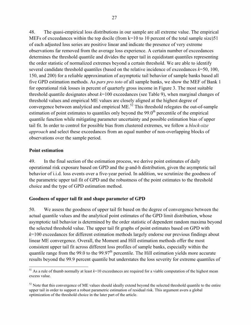
27

48. The quasi-empirical loss distributions in our sample are all extreme value. The empirical MEFs of exceedances within the top docile (from k=10 to 10 percent of the total sample size)51 of each adjusted loss series are positive linear and indicate the presence of very extreme observations far removed from the average loss experience. A certain number of exceedances determines the threshold quantile and divides the upper tail in equidistant quantiles representing the order statistic of normalized extremes beyond a certain threshold. We are able to identify several candidate threshold quantiles (based on the relative incidence of exceedances k=50, 100, 150, and 200) for a reliable approximation of asymptotic tail behavior of sample banks based all five GPD estimation methods. As pars pro toto of all sample banks, we show the MEF of Bank 1 for operational risk losses in percent of quarterly gross income in Figure 3. The most suitable threshold quantile designates about k=100 exceedances (see Table 9), when marginal changes of threshold values and empirical ME values are closely aligned at the highest degree of convergence between analytical and empirical ME.52 This threshold relegates the out-of-sample estimation of point estimates to quantiles only beyond the 99.0th percentile of the empirical quantile function while mitigating parameter uncertainty and possible estimation bias of upper tail fit. In order to control for possible bias from clustered extremes, we follow a block-size approach and select these exceedances from an equal number of non-overlapping blocks of observations over the sample period. Point estimation 49. In the final section of the estimation process, we derive point estimates of daily operational risk exposure based on GPD and the g-and-h distribution, given the asymptotic tail behavior of i.i.d. loss events over a five-year period. In addition, we scrutinize the goodness of the parametric upper tail fit of GPD and the robustness of the point estimates to the threshold choice and the type of GPD estimation method. Goodness of upper tail fit and shape parameter of GPD 50. We assess the goodness of upper tail fit based on the degree of convergence between the actual quantile values and the analytical point estimates of the GPD limit distribution, whose asymptotic tail behavior is determined by the order statistic of dependent random maxima beyond the selected threshold value. The upper tail fit graphs of point estimates based on GPD with k=100 exceedances for different estimation methods largely endorse our previous findings about linear ME convergence. Overall, the Moment and Hill estimation methods offer the most consistent upper tail fit across different loss profiles of sample banks, especially within the quantile range from the 99.0 to the 99.97th percentile. The Hill estimation yields more accurate results beyond the 99.9 percent quantile but understates the loss severity for extreme quantiles of 51 As a rule of thumb normally at least k=10 exceedances are required for a viable computation of the highest mean excess value. 52 Note that this convergence of ME values should ideally extend beyond the selected threshold quantile to the entire upper tail in order to support a robust parametric estimation of residual risk. This argument avers a global optimization of the threshold choice in the later part of the article.

28

99.99 percent or higher (similar to Moment method). The remaining estimation methods (MLE, Pickands and Drees-Pickands) overestimate actual losses but provide a slightly better specification of conditional mean excess within the quantile range from the 99.5th to 99.97th percentile. The Philips-Loretan (PL) (1990) estimation of the shape parameter tends to improve analytical point estimates of the Moment (and MLE) methods at the 99.9th percentile at the expense of less accurate upper tail fit. 51. Given the persistence of asymptotic tail convergence of the simulated loss probability density across different levels of reported gross income and the stability of quarterly and annual loss frequency over the sample period, we expect the original GEV shape parameter 1.0ξ = to be largely unchanged for GPD. Nonetheless, we observe a significant differences of shape parameter estimates across banks and estimation methods (see Table 11), mainly because, in some instances (e.g. for Bank 3), the occurrence of extremely large operational risk losses coincides with quarters of below-average gross income, amplifying relative operational risk exposure. The dispersion of the most extreme observations also influences the optimization of the GPD estimation method. The Pickands and the Drees-Pickands estimation methods generate shape parameter values of around 1.15, well above those derived from the Moment and MLE methods, as the former approach assigns more (tail) weight to the most extreme observations and supports a high shape parameter value (or small tail index) with a lower velocity of asymptotic tail decay.53 Estimation results 52. We summarize the results of the quantile point estimation of operational risk exposure based on GEV and GPD (“EVT-VaR”) and the g-and-h distribution fitted simulated loss data over a five-year risk horizon (see Tables 8 to 10). While a generalized assumption about extreme tail behavior (GEV) tends to overstate actual losses at high quantiles, the POT method of GPD for normalized i.i.d. maxima in excess of the designated sample threshold accurately represents the residual risk in the upper tail of the sample loss distributions. The quality of the parametric fit, however, varies by estimation method and percentile level of statistical confidence. For all banks, we observe a precipitous increase of empirical quantile values (i.e., observed operational risk losses) over the selected percentile range from 95.0 to 99.999 percent. The rate of change varies by bank and depends largely on the loss variance, which gradually increases from Bank 1 to Bank 4. The Moment and MLE methods substantiate the most consistent and stable GPD estimation for the at the 95th percentile or higher, irrespective of loss distribution characteristics. However, for the AMA-required probability level of 99.9 percent, only the inclusion of the PL method for the estimation of the shape parameter generates the best analytical point estimates (if combined with the Moment or MLE estimation methods) of the historical operational risk exposure, which ranges between 0.61 percent (Bank 1) and 2.39 percent (Bank 4) of gross income (per quarter). We also examine the effect of the risk horizon on the accuracy and the magnitude of accumulated

53 The Pickands and the Drees-Pickands estimation methods estimate tail decay based on the logarithmic differences between successive order statistics of the largest observations and the threshold value, whereas the former methods approximate asymptotic tail behavior over incremental ranges of order statistics of exceedances.

29

losses by deriving risk estimates for a single year worth of loss data (in lieu of a five-year estimation horizon) generated as i.i.d. random draws from a known probability function of loss severity. We find that the accumulation of losses over multiple years masks considerable variability of estimated operational risk exposure (see Table 10), partly caused by the aggregate sample statistics of LDCE (see Tables 2 and 3). The risk horizon amplifies the sensitivity of the goodness of upper tail fit to the percentile level and increases estimation risk and parameter uncertainty due to intermittent annual loss frequency and variable loss skewness (including the inconsistent identification of extremes). The final year of simulated losses offers the most robust and consistent GPD estimates of any sample year. In view of the considerable data limitations, a risk-horizon of at least three years appears sensible based on the average historical loss experience of U.S. commercial banks. 53. GEV and GPD exhibit upper tail convergence that is largely distinct from the g-and-h distribution. GPD supports the closest approximation of actual quantiles, especially when point estimates of the aggregate loss series are derived “within the sample” at around the 99.0th percentile. The g-and-h distribution substantiates the most consistent upper tail fit and outperforms GPD for the most extreme quantiles of 99.99 percent and higher, whose residual risk tends to be grossly overstated by POT. The point estimates of the g-and-h distribution are also particularly stable and accurate around the 97.5th percentile, which roughly coincides with the optimal threshold quantile for the most reliable specification of conditional mean excess under GPD (see Table 14). Nonetheless, around the critical 99.9th percentile, risk estimates under GPD are superior to those generated by the g-and-h distribution (which seem to be more aligned to the normal distribution at this level of statistical confidence). Our estimation results suggest that GPD and the g-and-h distribution are complementary. While POT under GPD delivers reasonably accurate and robust point estimates for sufficiently large sample sizes, the g-and-h distribution seems more appropriate for very extreme quantiles that are notorious for out-of-sample estimation when the loss sample is small or point estimates are derived over shorter risk horizons (and a low attendant loss threshold) (see Table 10). These findings of optimal model specification of residual risk underscore the delicate trade-off between measurement objectives and parameter stability when parametric fitting based on order statistics displaces more rigorous estimation methods in absence of appropriate back-testing procedures to determine exposures far removed from the historical loss experience. In the next section, we propose several robustness tests in order to illustrate the model sensitivity of point estimates to the threshold choice at different levels of statistical confidence.

K. Robustness of GPD Point Estimates to Threshold Choice 54. So far, we have achieved convergence of asymptotic tail behavior to GPD based on a selection of extremes beyond the highest possible threshold that still yields (I) linear conditional ME consistent with the external types theorem of GEV and (ii) a stable parametric upper tail fit. However, the POT-based estimation of the first three moments of GPD considers all designated extremes over the entire upper tail, which fails to ascertain the joint effect of both variable levels of loss thresholds and desired statistical confidence on the accuracy of individual point estimates. Therefore, a global threshold choice appears to be inadequate for the optimal specification of

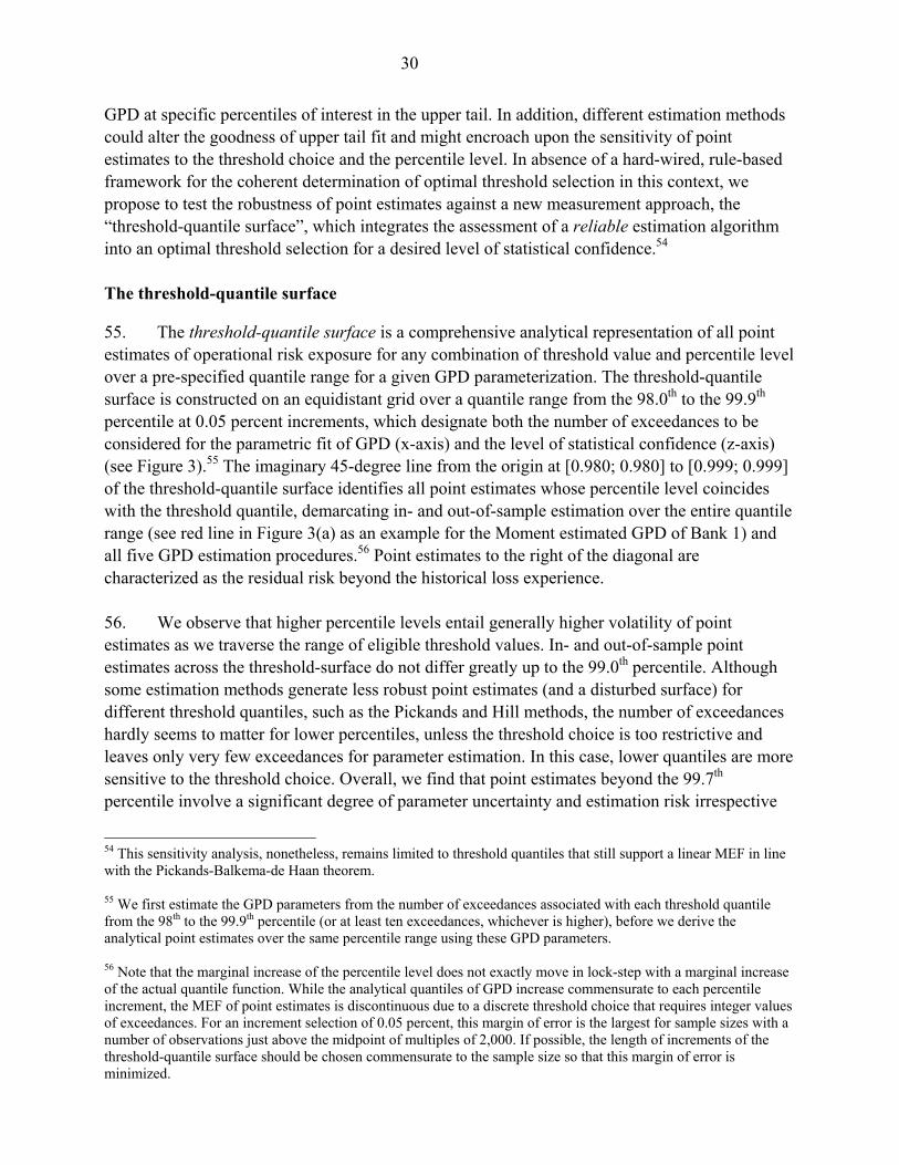
30

GPD at specific percentiles of interest in the upper tail. In addition, different estimation methods could alter the goodness of upper tail fit and might encroach upon the sensitivity of point estimates to the threshold choice and the percentile level. In absence of a hard-wired, rule-based framework for the coherent determination of optimal threshold selection in this context, we propose to test the robustness of point estimates against a new measurement approach, the “threshold-quantile surface”, which integrates the assessment of a reliable estimation algorithm into an optimal threshold selection for a desired level of statistical confidence.54 The threshold-quantile surface 55. The threshold-quantile surface is a comprehensive analytical representation of all point estimates of operational risk exposure for any combination of threshold value and percentile level over a pre-specified quantile range for a given GPD parameterization. The threshold-quantile surface is constructed on an equidistant grid over a quantile range from the 98.0th to the 99.9th percentile at 0.05 percent increments, which designate both the number of exceedances to be considered for the parametric fit of GPD (x-axis) and the level of statistical confidence (z-axis) (see Figure 3).55 The imaginary 45-degree line from the origin at [0.980; 0.980] to [0.999; 0.999] of the threshold-quantile surface identifies all point estimates whose percentile level coincides with the threshold quantile, demarcating in- and out-of-sample estimation over the entire quantile range (see red line in Figure 3(a) as an example for the Moment estimated GPD of Bank 1) and all five GPD estimation procedures.56 Point estimates to the right of the diagonal are characterized as the residual risk beyond the historical loss experience. 56. We observe that higher percentile levels entail generally higher volatility of point estimates as we traverse the range of eligible threshold values. In- and out-of-sample point estimates across the threshold-surface do not differ greatly up to the 99.0th percentile. Although some estimation methods generate less robust point estimates (and a disturbed surface) for different threshold quantiles, such as the Pickands and Hill methods, the number of exceedances hardly seems to matter for lower percentiles, unless the threshold choice is too restrictive and leaves only very few exceedances for parameter estimation. In this case, lower quantiles are more sensitive to the threshold choice. Overall, we find that point estimates beyond the 99.7th percentile involve a significant degree of parameter uncertainty and estimation risk irrespective

54 This sensitivity analysis, nonetheless, remains limited to threshold quantiles that still support a linear MEF in line with the Pickands-Balkema-de Haan theorem. 55 We first estimate the GPD parameters from the number of exceedances associated with each threshold quantile from the 98th to the 99.9th percentile (or at least ten exceedances, whichever is higher), before we derive the analytical point estimates over the same percentile range using these GPD parameters. 56 Note that the marginal increase of the percentile level does not exactly move in lock-step with a marginal increase of the actual quantile function. While the analytical quantiles of GPD increase commensurate to each percentile increment, the MEF of point estimates is discontinuous due to a discrete threshold choice that requires integer values of exceedances. For an increment selection of 0.05 percent, this margin of error is the largest for sample sizes with a number of observations just above the midpoint of multiples of 2,000. If possible, the length of increments of the threshold-quantile surface should be chosen commensurate to the sample size so that this margin of error is minimized.

31

of threshold choice. Lower threshold values are more “forgiving” but tend to slightly overstate loss severity. Lower quantiles also involve less estimation risk if at least 0.2 percent of all observations are classified as exceedances. All threshold-quantile surface estimations indicate the most consistent estimation results around the 99.0th percentile, confirming earlier findings. Consolidating one dimension of the threshold-quantile surface 57. We can simplify the illustration of the contemporaneous effect of threshold choice and percentile level on the accuracy and order of magnitude of point estimates by collapsing one dimension of the threshold-quantile surface into a descriptive statistic of parameter sensitivity. We consolidate the z-axis of percentile levels into a descriptive statistic of the upper tail shape in order to show the aggregate sensitivity of point estimates in the upper tail (and the accuracy of constituent point estimates) to a defined range of threshold quantiles. Similarly, consolidating the x-axis of different threshold quantiles yields the aggregate sensitivity of point estimates to a variable threshold choice at each percentile level of the upper tail. For each approach, we also calculate (I) the relative deviation of the estimated from the actual upper tail shape at each threshold quantile (see Figure 4) and (ii) the relative deviation of point estimates from the actual quantile values as we traverse the percentile range of the upper tail (see Figure 5). 58. We find that point estimates are affected differently by the degree of parameter stability in response to a gradual change of the loss threshold. The sensitivity of upper tail fit to the number of exceedances is marginal for threshold quantiles between the 98.0th and the 99.7th percentile, whereas higher thresholds increase the scope for parameter uncertainty from out-of-sample estimation. That said, the positive correlation between the threshold quantile and the deviation of the estimated from the actual median of the upper tail testifies to greater variation of point estimates as fewer observations are designated as exceedances (see Table 12). Conversely, point estimates appear to be more sensitive to changes of the desired level of statistical confidence if the threshold quantile is kept completely flexible (see Figure 5). The positive correlation between the deviation of the median point estimate from the actual quantile value and the threshold quantile flags greater estimation risk as we traverse the upper tail (see Table 13). If we ignore the extreme results for the 99.9th threshold quantile (which are largely explained by an insufficient number of exceedances for reliable estimation), the selection of the right percentile level rather than the threshold choice (within a high threshold quantile range) seems to matter most for robust point estimates and optimal parametric GPD-based upper tail fit. Limiting one dimension of the threshold-quantile surface to a specific threshold or percentile level 59. As an alternative simplification, we disregard one dimension of the threshold-quantile surface altogether if the choice of a percentile level for point estimates is pre-determined or data limitations restrict the loss threshold to a particular quantile only. Thus, we devise the single point estimate graph and the single threshold upper tail graph as a two-dimensional rendition of the threshold-quantile surface for a particular percentile level (over a continuous range of thresholds) or threshold quantile (over a percentile range of statistical confidence) respectively. In

32

contrast to the consolidation of the upper tail or the threshold quantile range in the previous section, the focus on only one percentile level or threshold quantile allows a straightforward comparative analysis of different GPD estimation algorithms. 60. Our approach of leaving the percentile level unchanged concurs with AMA soundness standards. Banks using GPD as LDA for AMA would a natural tendency to optimize the choice of both loss threshold and estimation method to achieve the closest upper tail fit with reliable point estimates at the 99.9th percentile of statistical confidence. Figure 6 shows a panel of three single point estimate graphs of all estimation methods for single percentile levels over a continuous threshold choice within the quantile range from 99.7th to the 99.5th percentile, which is equivalent to a “horizontal slice” along the threshold range (x-axis) at the selected percentile level of the threshold-quantile surface. Although the individual sensitivity of point estimates to an increasing threshold is distinct for each estimation method, the general pattern of variation hardly varies across the different percentile levels. Moment and MLE estimation methods with Philips-Loretan (PL) produce the most consistent point estimates within a “comfort zone” of threshold quantiles between the 98.5th and the 99.0th percentile. 61. Scarce historical loss data could also warrant the quantification of operational risk contingent on a predetermined threshold quantile that qualifies extreme events. Figure 8 shows a panel of single threshold upper tail graphs of point estimates based on three different loss thresholds over an upper tail range from the 99.75th to the 99.99th percentile. As a subset of the threshold-quantile surface, each graph represents a “vertical slice” along the percentile range (z-axis) at the selected threshold level. The shape of the upper tail fit to the empirical distribution varies by estimation method and exhibits distinct convexity, which declines at higher thresholds. A threshold quantile around the 99.0th percentile offers the most reliable results, particularly for the Moment and the MLE estimation method with and without PL estimated tail shape.

L. Backward Induction of Optimal Threshold Choice 62. For purposes of an improved point estimation under GPD, the threshold-quantile surface method also informs an integrated optimization of threshold selection through backward induction either (I) at any percentile level within the upper tail (global optimization) or (ii) at a certain, pre-defined percentile level (local optimization) based on a specific parametric estimation of GPD. While the global optimization selects combinations of threshold quantiles and estimation methods that engender the most consistent upper tail fit of point estimates (i.e., consolidated z axis of the threshold-quantile surface) (see Figure 5 as well as Table 12), local optimization identifies a threshold quantile that minimizes the deviation of point estimates from actual values at a specific percentile level (i.e., single point estimate graph) (see Figures 6 and 7). Conversely, the sensitivity of individual point estimates to a flexible threshold choice either at each percentile level within the upper tail (see Figure 4 and Table 13) or at a specific percentile level (i.e., single threshold upper tail graph (see Figures 8 and 9) complements these analyses. Table 14 summarizes our findings within the overall analysis of our GPD estimation results.

33

Local threshold optimization 63. Given our interest in a particular percentile p of the loss distribution operational risk exposure, the single point estimate graph lies at the heart of the local optimization of the threshold choice at the 99.9th percentile. The following procedure encapsulates a reliable selection of both threshold quantile and estimation method for point estimates at a specific percentile level. We first choose the most consistent GPD estimation method that generates point estimates with the lowest sensitivity to a variable threshold between the 97.0th and the 99.5th percentile (see Table 14(5)). We then select the local threshold quantile *

lq , which engenders the smallest deviation of the point estimate from the actual quantile value (see Table 14(6)). Finally, we qualify *

lq on the smallest joint divergence of point estimates over different estimation methods (see Table 14(7)) in order to reign in potential bias from a particular estimation method. We complement the optimization of a local threshold with the sensitivity analysis of upper tail fit over a certain percentile range to a specific threshold quantile q close to the optimal local threshold *

lq . The single threshold upper tail graph identifies the optimal local percentile level

( )*lp . We find that there are decreasing marginal benefits from higher thresholds to support point

estimates at a high levels of statistical confidence according to AMA standards. Risk estimates at the critical percentile level of p=99.9 percent of AMA are most accurate for threshold quantiles

*lq ranging from 97.52 percent to 98.78 percent, depending on the estimation method and sample

bank. Since higher percentiles would require disproportionately more loss data to support a higher loss threshold that maintain linear ME of exceedances, stringent regulatory requirements at high percentile levels impose an implicit limit on potential capital savings from adopting AMA amid notoriously scarce historical operational risk loss data. 64. We refine an optimal local threshold on a conditional and an unconditional measure. The unconditional local threshold choice ( )*

,l uq supports the closest alignment of a single point

estimate to the actual value across all estimation methods (see Table 14(8)), regardless of the consistency of overall upper tail fit (see Table 14(5). Similar to the general optimization procedure above, we also complete the unconditional optimization of a local percentile level

( )*,l up based on the single threshold upper tail graph (see Table 14(13)). Without the restriction

of an estimation method on the most consistent upper tail fit, the optimal threshold declines significantly to around the 98.0th percentile. However, the percentile levels remain largely unchanged between the conditional and unconditional optimization, with the latter generating more accurate point estimates. We condition *

,l uq on the estimation method that generates the best overall upper tail fit (see Table 14(1)) based on conventional threshold diagnostics that ascertain compliance of the ME of identified exceedances with the Pickands-Balkema-de Haan limit theorem (see Table 8 and Figure 2). We finally augment the conditional optimization of the local threshold choice *

,l cq (see Table 14(9)) by the influence of the desired percentile level of point

estimates in the form of the conditional optimization of a local percentile level *,l cp (see Table

14(14)). Despite higher threshold quantiles, the conditional optimization engenders a more

34

balanced trade-off between the threshold and the percentile levels, i.e., an increase of the loss threshold translates into a matching increase of statistical confidence of point estimates at the margin. Most importantly, the conditional optimization at p=99.9 percent identifies a local threshold *

,l cq that corresponds to the deterministic threshold quantile q=99.0 percent for the

optimal local percentile *,l cp , suggesting complementary optimization.

Global threshold optimization 65. The optimization of a local threshold at a particular ex ante percentile level fails to inform a general threshold choice for optimal upper tail fit at different percentile levels as much as the general optimization of a local percentile for a specific threshold cannot identify a general percentile level over a range of threshold quantiles consistent with an optimal local threshold. In contrast, the combination of the conditional optimization of a global threshold and a global percentile level considers the joint sensitivity of point estimates to both threshold and percentile level (see Table 11). A global threshold *

,g cq (see Table 14(15)) minimizes the difference between the median point estimate and the actual median value of the upper tail (see Figure 7 and Table 12) based on the estimation method for the best original upper tail fit (see Table 14(1)). We find that *

,g cq almost always concurs with *,l cq (see Table 14(9)). However, without imposing

restrictions on the permissible estimation method, *,g cq is much higher than *

,l uq (see Table 14(8)).

A global percentile level *,g cp for best upper tail fit minimizes the difference between the actual

percentile value and the dispersion of point estimates over the entire range of thresholds at a certain level of statistical confidence (see Figure 9). Hence, by keeping the threshold choice variable, we can determine the percentile level (see Table 14(16)) at which point estimates are least sensitive to the threshold choice (see Table 13). Our estimates largely support previous results (see Table 14(4)), which showed that point estimates below the 99.0th percentile are least sensitive to the threshold choice. The combination of *

,g cq and *,g cp also reveals that the most

reliable estimation of quasi-empirical losses for the best overall upper tail fit requires in-sample estimation for all but one sample bank. Although point estimates appear to be less sensitive to the threshold choice than varying percentile levels after all, insufficient observations of extremes preclude thresholds that support reliable, in-sample upper tail fit as the level of statistical confidence increases.

VI. CONCLUSION 66. In this paper, we investigated the economic and regulatory implications of modeling operational risk in compliance with the regulatory capital standards set forth by the New Basel Capital Accord. We identified GEV, GPD, and the g-and-h distribution as feasible measurement approaches to assess the generalized parametric specification of the fat-tailed limiting behavior commonly associated with large operational risk losses. Our estimation quantified the hypothetical impact of unexpected operational risk losses (UL) on the financial performance of a selected set of U.S. commercial banks and indicated whether current capital rules establish an

35

adequate framework for the realistic and consistent regulatory treatment of operational risk. Although we primarily focused on the optimal GPD-based specification of tail dependence (including comprehensive threshold diagnostics using an integrated analysis of mean excess, the stability of the tail index parameter, and the goodness of upper tail fit), we also derived in- and out-of-sample point estimates of operational risk exposure for parametric specification of GEV and the g-and-h distribution. Finally, we examined the sensitivity risk estimates to different loss thresholds and percentile levels in order to ascertain the robustness of our results given the inherent instability of tail convergence under GPD. 67. Based on our sample of simulated operational risk losses adjusted by quarterly reported gross income, the impact of operational risk on fundamental performance seems minimal at the 99.9th percentile level required by AMA standards. The bank with the most distinct low-frequency, high-severity loss profile would have lost only 1.75 percent of gross income over a five year horizon, while standardized approaches of current operational risk regulation would have required a fixed capital charge of 15 percent of three-year average gross income. These descriptive statistics challenge the business-volume dependence of operational risk and show that gross income as a volume-based metric seems inadequate for an equitable treatment of operational risk under different regulatory risk measurement approaches. Although the New Basel Capital Accord recognizes considerable variation of relative loss severity of operational risk events within and across banks, the economic logic of volume-based measures collapses in cases when banks incur small (large) operational risk losses in Bless where an aggregate volume-based measure would indicate high (low) operational risk exposure. 68. Overall, large differences between AMA risk estimates and capital charge under standardized approaches (BIA and TSA) hint at prima facie inconsistency of operational risk measurement under the current regulatory framework if we ascribe general empirical validity to our loss data. At an uniform capital charge of 15 percent of average annual gross income, AMA would require much higher levels of statistical confidence (of at least 99.99 percent) to engender loss severity comparable to standardized measures (at the expense of higher estimation risk and parameter uncertainty of analytical methods). In light of the notorious scarcity of historical data on operational risk losses, only a lower fixed capital multiplier of standardized approaches would be consistent with AMA at the current level of required statistical confidence. 69. We found that AMA-compliant risk estimates of operational risk under both EVT and the g-and-h distribution generated reliable and realistic estimates of UL. Compared to Mignola and Ugoccioni (2006), our parametric specification entailed a lower estimation error and closer upper tail convergence, partly because we did not calibrate the loss generating function to the standardized regulatory capital charge for operational risk. Our parametric risk estimates of i.i.d. normalized maxima at the required 99.9th percentile implied capital savings of up to almost 97 percent compared to an uniform measure of operational risk exposure. Although the g-and-h distribution (and its power law variant)57 outperformed both GEV and GPD in terms of the

57 In this approach, high quantiles of the aggregate loss distribution can be calculated analytically by a scaled multiplication of the largest order statistic, provided that the largest observations follow a power law.

36

goodness of upper tail fit, our results do not corroborate the 16.79 percent capital-to-gross income ratio in Dutta and Perry, 2006.58 In fact, the g-and-h distribution underestimated actual losses in all but the most extreme quantiles of 99.95 percent and higher, when EVT-based estimates overstated excess elongation of asymptotic tail decay. Our findings suggest a symbiotic association between EVT and the g-and-h distribution for optimal point estimation depending on the percentile level and the incidence of extreme events. 70. Parameter instability at high percentile levels is largely caused by the lack of sufficient empirical loss data, which permit only simple parametric models of asymptotic tail behavior. In this case, GPD proves to be the most useful method to derive “out-of-sample” estimates of asymptotic tail behavior—after comprehensive sensitivity analysis. Despite its close empirical approximation at an average deviation of only about 10–25 percent across the upper tail, however, the application of EVT warrants a careful assessment of estimation risk at different levels of statistical confidence for different estimation methods, loss thresholds, and loss profiles. In a bid to determine a consistent measure of operational risk across seven banks, Dutta and Perry (2006) found GPD to be inadequate as a general benchmark model due to an overestimation in small samples.59 Their results concurred with Mignola and Ugoccioni (2005), who showed that the rate of convergence of the shape parameter can be poor, even for reasonably large samples.60 However, since the scarcity of actual loss data defies back-testing for very extreme quantiles, discussions about optimal upper tail fit under different distributions—especially across different banks—cannot be robust much less exhaustive. Even the extensive LDCE data gathered by U.S. banking regulators prove insufficient to sustain comparability of point estimates across different loss distributions at the 99.9th percentile. 71. In the effort to curb parameter uncertainty of GPD, we introduced the concept of the “threshold-quantile surface” as an integrated approach to illustrate the contemporaneous effect of the threshold choice, the estimation method, and the desired statistical confidence on the accuracy of point estimates and upper tail fit. We found that the selection of the right percentile level rather than the threshold choice seemed to matter most for robust point estimates of aggregate operational risk. Estimation uncertainty increased significantly at high levels of statistical confidence beyond the 99.7th percentile or threshold quantiles that classified less than 0.5 percent of all losses as exceedances for the parametric GPD-based upper tail fit. A marginal drop of the 58 This divergence from our results could in part have resulted from their choice of the Hill algorithm as GPD estimation method. Mittnick and Rachev (1996) found that the Hill estimation algorithm yields highly unstable estimates of upper tail shape for samples with less than 500,000 observations. Moreover, the Hill estimation method returns inaccurate results of asymptotic tail behavior for distributions with a non-zero left endpoint, which is the case in Dutta and Perry (2006), who use LDCE loss data only from banks with a reported loss threshold of at least US$10,000. 59 Sweeping assertions of unreliable GPD estimates are contestable and need to be qualified on the joint effect of loss threshold and desired percentile level of point estimates for different estimation algorithms. 60 Degen et al. (2006) also flagged the possibility of inaccurate results due to a slowly converging excess distribution of extremes, but also caution that alternative modeling by means of the g-and-h distribution entails considerable parameter risk arising from the quantile-based estimation of higher moments.

37

regulatory loss quantile from 99.9 percent to 99.7 percent entailed a disproportional reduction of both UL and the optimal threshold quantile at lower estimation uncertainty but far smaller sample sizes of required loss data. We obtained the most reliable and exact parametric specification under GPD, if we considered the Moment and MLE estimation methods for the approximation of the asymptotic tail behavior of extremes beyond a threshold quantile of about 98.5 percent and a statistical confidence level of no higher than 99.0 percent, regardless of varying tail shape properties of different loss profiles. Our findings suggest that AMA criteria seem to have been set deliberately beyond the historical loss experience of banks in order to encourage the combination of different internal measurement models and the creation of capital buffers. 72. The cross-sectional variation of loss profiles and the trade-off between reliability and accuracy of risk estimates underscore an inherent joint hypothesis problem of operational risk measurement—either the model is correct and the testable data is not or vice-versa. AMA yields more accurate estimates of unexpected operational risk and appeal to the usage of economic capital as determinant of banking performance, but it fails to address structural and systemic effects of heterogeneous loss data. The standardization of units of measure notwithstanding, consistent AMA estimation might be compromised by cross-sectional variation of reported loss frequency and incentives of loss fragmentation. Normative assumptions eschew such measurement bias in favor of greater reliability—but they do so at the expense of less discriminatory power and higher capital charges. 73. A revised regulatory framework for operational risk would benefit from a comparative assessment of the time-varying impact of different loss profiles of banks under different measurement approaches. Despite the analytical benefits of upper tail specification based on order statistics, the most common measurement models used by banks do not identify the incidence of extremes as a dynamic process. Since one-off operational risk events also elude purely quantitative models, sound risk measurement would also require a qualitative overlay, whose prominence needs to be carefully balanced with a considerable degree of judgment and mindful interpretation of historical precedence. 74. Following this paper, some of the future terrain to be covered should include a detailed analysis of joint dependence of extremes based on multivariate EVT approaches in order to assess alleged correlation effects across different units of measure. In this context, loss estimates could also be shown to exhibit granularity to capture risk drivers in a structural model specification. Moreover, the circumspect investigation of different modes of reporting operational risk losses in terms of timing and organizational detail could help derive regulatory controls of self-assessment, which promote consistent sensitivity measures of the loss severity and loss frequency. A logical extension of our approach would also include a more extensive application of the g-and-h distribution across different loss profiles of banks (Dutta and Perry, 2006; Degen et al., 2006). Finally, it might be useful to develop d an optimization algorithm for the “threshold-quantile surface” in the spirit of the Danielsson et al. (2001) bootstrap method to objectively choose a threshold level based on a bias-variance trade-off.

38

REFERENCES Adler, Robert J., Feldman, Raisa E. and Murad S. Taqqu, 1998, A Practical Guide to Heavy

Tails, Statistical Techniques and Applications, Birkhäuser, Boston-Basel-Berlin. Alexander, Carol (ed.), 2003. Operational Risk: Regulation, Analysis and Management.

Financial Times—Prentice Hall, London. Anonymous, 2007, “Capital Standards: Proposed Interagency Supervisory Guidance for Banks

That Would Operate Under Proposed New Basel II Framework,” US Fed News (28 February).

Badrinath, Swaminathan G. and Sangit Chatterjee, 1991, “A Data-Analytic Look at Skewness

and Elongation in Common-Stock Return Distributions,” Journal of Business and Economic Statistics, Vol. 9, No. 9, 223–33.

Badrinath, Swaminathan G. and Sangit Chatterjee, 1988, “On Measuring Skewness and

Elongation in Common Stock Return Distributions: The Case of the Market Index,” Journal of Business, Vol. 61, No. 4, 451–72.

Balkema, August A. and Laurens de Haan, 1974, “Residual Life Time at Great Age,” Annals of

Probability, Vol. 2, 792–804. Banerjee, Suman and Kulwinder Banipal, 2005, “Managing Operational Risk: Framework for

Financial Institutions,” Working paper, A.B Freeman School of Business, Tulane University (November).

Basel Committee on Banking Supervision, 2006a, Observed Range of Practice in Key Elements

of Advanced Measurement Approaches (AMA). BCBS Publications No. 131, Bank for International Settlements,(October), (http://www.bis.org/publ/bcbs131.htm).

Basel Committee on Banking Supervision, 2006b, Basel II: International Convergence of Capital

Measurement and Capital Standards: A Revised Framework—Comprehensive Version. BCBS Publications No. 128, Bank for International Settlements,(June), (http://www.bis.org/publ/bcbs128.htm).

Basel Committee on Banking Supervision, 2005, Basel II: International Convergence of Capital

Measurement and Capital Standards: A Revised Framework, Bank for International Settlements, (November), (http://www.bis.org/publ/bcbs118.htm).

Basel Committee on Banking Supervision, 2004, International Convergence of Capital

Measurement and Capital Standards: A Revised Framework, Bank for International Settlements, (June), (http://www.bis.org/publ/bcbs107.htm).

39

Basel Committee on Banking Supervision, 2003a, Operational Risk Transfer Across Financial Sectors, Joint Forum Paper, Bank for International Settlements, (August), (http://www.bis.org/publ/joint06.htm).

Basel Committee on Banking Supervision, 2003b, Sound Practices for the Management and

Supervision of Operational Risk, BCBS Publications No. 96, Bank for International Settlements, (February), (http://www.bis.org/publ/bcbs96.htm).

Basel Committee on Banking Supervision, 2002, Sound Practices for the Management and

Supervision of Operational Risk, BCBS Publications No. 91, Bank for International Settlements, (July), (http://www.bis.org/publ/bcbs91.htm).

Basel Committee on Banking Supervision, 2001a, Sound Practices for the Management and

Supervision of Operational Risk, BCBS Publications No. 86, Bank for International Settlements, (December), (http://www.bis.org/publ/bcbs86.htm).

Basel Committee on Banking Supervision, 2001b, Working Paper on the Regulatory Treatment

of Operational Risk. BCBS Publications No. 8, Bank for International Settlements, (September), (http://www.bis.org/publ/bcbs_wp8.pdf).

Basel Committee on Banking Supervision, 2001c, Consultative Document—Operational Risk

(Supporting Document to the New Basel Capital Accord), BCBS Publications (Consultative Document), No. 7, Bank for International Settlements, (January), (http://www.bis.org/publ/bcbsca07.pdf).

Basel Committee on Banking Supervision, 1998, Operational Risk Management, BCBS

Publications No. 42, Bank for International Settlements, (September), (http://www.bis.org/publ/bcbs42.htm).

Behrens, Cibele N., Lopes, Hedibert F. and Dani Gamerman, 2004, “Bayesian Analysis of

Extreme Events with Threshold Estimation,” Working paper, Federal University of Rio de Janeiro, Department of Economics.

Beirlant, Jan, Dierckx, Goedele, Goegebeur, Yuri and Gunther Matthys, 1999, “Tail Index

Estimation and an Exponential Regression Model,” Extremes, Vol. 2, 77–200. Beirlant, Jan, Vynckier, Petra, and Jozel L. Teugels, 1996, “Tail Index Estimation, Pareto

Quantile Plots, and Regression Diagnostics,” Journal of the American Statistical Association, Vol. 91, 1659–67.

Bensalah, Younes, 2000, “Steps in Applying Extreme Value Theory to Finance: A Review,”

Working Paper 2000–20, Bank of Canada.

40

Bermudez, P. de Zea, Amaral Turkman, Maria A., and Kamil F. Turkman, 2001, “A Predictive Approach to Tail Probability Estimation,” Extremes, Vol. 4, 295–314.

Castillo, Enrique and Ali S. Hadi, 1997, “Fitting the Generalized Pareto Distribution to Data,”

Journal of the American Statistical Association, Vol. 92(440), 1609–20. Chernobai, Anna, and Svetlozar Rachev, 2006, “Applying Robust Methods to Operational Risk

Modeling,” Journal of Operational Risk, Vol. 1, 27–41. Cohen, Jonathan P., 1982a, “The Penultimate Form of Approximation to Normal Extremes,”

Advances in Applied Probability, Vol. 14, 324–39. Cohen, Jonathan P., 1982b, “Convergence Rates for the Ultimate and Penultimate

Approximations in Extreme Value Theory,” Advances in Applied Probability, Vol. 14, 833–54.

Coleman, Rodney and Marcelo Cruz, 1999, “Operational Risk Measurement and Pricing,”

Derivatives Week, Vol. 8, No. 30, (July 26), 5–6. Coles, Stuart G., 2001, An Introduction to Statistical Modeling in Extreme Values, Springer

Verlag, London. Coles, Stuart G., Heffernan, Janet, and Jonathan A. Tawn, 1999, “Dependence Measures for

Extreme Value Analyses,” Extremes, Vol. 2, 339–65. Crouhy, Michel, Galai, Dan, and Mark M. Robert, 2004, “Insuring versus Self-Insuring

Operational Risk: Viewpoints of Depositors and Shareholders,” Journal of Derivatives, (Winter), Vol. 12, No. 2, 51–5.

Cruz, Marcelo, Coleman, Rodney and Gerry Salkin, 1998, “Modeling and Measuring Operational

Risk,” Journal of Risk, Vol. 1, No. 1, 63–72. Danielsson, Jon, de Haan, Laurens, Peng, Liang, and Casper G. de Vries, 2001, “Using a

Boostrap Method to Choose a Sample Fraction in Tail Index Estimation,” Journal of Multivariate Analysis, Vol. 76, 226–48.

Danielsson, Jon and Casper G. de Vries, 1997a, “Tail Index and Quantile Estimation With Very

High Frequency Data,” Journal of Empirical Finance, Vol. 4, 241–57. Danielsson, Jon and Casper G. de Vries, 1997b, “Extreme Returns, Tail Estimation, and Value-

at-Risk,” Working paper presented at a conference on Issues in Empirical Finance, organized by LSE Financial Markets Group, (November 21–22).

41

Degen, Matthias, Embrechts, Paul, and Dominik D. Lambrigger, 2006, “The Quantitative Modeling of Operational Risk: Between g-and-h and EVT,” Working paper, ETH Preprint, Zurich, (December 19).

Dekkers, Arnold L. M., and Laurens de Haan, 1989, “On the Estimation of Extreme-Value Index

and Large Quantile Estimation,” Annals of Statistics, Vol. 17, 1795–1832. Dekkers, Arnold L. M., Einmahl, John H. J., and Laurens de Haan, 1989, “A Moment Estimator

for the Index of an Extreme-Value Distribution,” Annals of Statistics, Vol. 17, 1833–55. Diebold, Francis X., Schürmann, and Til and John D. Stroughair, 1998, “Pitfalls and

Opportunities in the Use of Extreme Value Theory in Risk Management,” in: Refenes, A.-P. N., Moody, J. D., and A. N. Burgess (eds.), Advances in Computational Finance, Kluwer, Amsterdam, 3–12.

Drees, Holger, 1995, “Refined Pickands Estimators of the Extreme Value Index,” Annals of

Statistics, Vol. 23, 2059–80. Dutta, Kabir K. and David F. Babbel, 2005, “Extracting Probabilistic Information from the Prices

of Interest Rate Options: Test of Distributional Assumptions,” Journal of Business, Vol. 78, No. 3, 841–70.

Dutta, Kabir K. and David F. Babbel, 2002, “On Measuring Skewness and Kurtosis in Short Rate

Distributions: The Case of the US Dollar London Inter Bank Offer Rates,” Wharton Financial Institutions Center Working Paper.

Dutta, Kabir K. and Jason Perry, 2006, “A Tale of Tails: An Empirical Analysis of Loss

Distribution Models for Estimating Operational Risk Capital,” Working Paper No. 06–13 (July), Federal Reserve Bank of Boston.

Embrechts, Paul, 2000, “Extreme Value Theory: Potential and Limitations as an Integrated Risk

Management Tool,” Derivatives Use, Trading & Regulation, Vol. 6, 449–56. Embrechts, Paul, Hoenig, Andrea, and Alessandro Juri, 2003, “Using Copulae to Bound the

Value-at-Risk for Functions of Dependent Risk,” Finance and Stochastics, Vol. 7, No. 2, (April).

Embrechts, Paul, McNeil, Alexander, and Daniel Straumann, 2002, “Correlation and Dependence

in Risk Management: Properties and Pitfalls,” in M. Dempster (ed.), Risk Management: Value at Risk and Beyond, Cambridge University Press, 176–223.

Embrechts, Paul, Hoenig, Andrea, and Alessandro Juri, 2001a, “Using Copulae to Bound the

Value-at-Risk for Functions of Dependent Risk,” Preprint, ETH, Zurich.

42

Embrechts, Paul, Lindskog, Filip, and Alexander McNeil, 2001b, “Modelling Dependence with

Copulas and Applications to Risk Management,” Preprint, ETH, Zurich. Embrechts, Paul, Resnick, Sidney I., and Gennady Samorodnitsky, 1999, “Extreme Value Theory

as a Risk Management Tool,” North American Actuarial Journal, Vol. 26, 20–40. Embrechts, Paul, Klüppelberg, Claudia and Thomas Mikosch, 1997, Modelling Extremal Events

for Insurance and Finance, Springer-Verlag, Heidelberg. Falk, Michael, Hüsler, Jürg, and Rolf-Dieter Reiss, 1994, Laws of Small Numbers: Extremes and

Rare Events, DMV-Seminar, Birkhäuser, Basel. Federal Reserve Board, 2006, Fourth Quantitative Impact Study 2006, Washington, D.C.,

(http://www.federalreserve.gov/boarddocs/bcreg/2006/20060224/). Federal Reserve Board, 2004, Federal Reserve Statistical Release—Aggregate Reserves of

Depository Institutions and the Monetary Base, Washington, D.C. (http://www.federalreserve.gov/releases/h3/20050120).

Ferreira, Ana and Casper de Vries, 2003, “Optimal Confidence Intervals of the Tail Index and

High Quantiles,” Working paper (July 9), (http://home.isa.utl.pt/~anafh/ci.pdf). Fisher, Ronald Aylmer, and Leonard Henry Caleb Tippett, 1928, “Limiting Forms of the

Frequency Distribution of the Largest or Smallest Member of a Sample,” Proceedings of the Cambridge Philosophical Society, Vol. 24, 180–90.

de Fontnouvelle, Patrick, 2005, “The 2004 Loss Data Collection Exercise,” Presentation at the

Implementing an AMA for Operational Risk conference of the Federal Reserve Bank of Boston (May 19), (http://www.bos.frb.org/bankinfo/conevent/oprisk2005/defontnouvelle.pdf).

de Fontnouvelle, Patrick, Rosengren, Eric S., and John S. Jordan, 2004, “Implications of

Alternative Operational Risk Modeling Techniques,” SSRN Working Paper (June), (http://papers.ssrn.com/sol3/papers.cfm?abstract_id=556823).

Galambos, Janos, 1980, “A Statistical Test for Extreme Value Distributions,” Tech. Rep. 32,

Coll. Math, Soc. Janos, Bolyai, Budapest. Gnedenko, Boris V., 1943, “Sur la Distribution Limite du Terme Maximum d’Une Série

Aléatoire,” Annals of Mathematics, Vol. 44, 423–53.

43

Gomes, M. Ivette, 1982, “A Note on Statistical Choice of Extremal Models,” Tech. Rep., Act. IX, Jornadas Matemáticas Hispano-Lusas, Salamanca II.

Grody, Allan D., Harmantzis, Fotios C., and Gregory J. Kaple, 2005, “Operational Risk and

Reference Data: Exploring Costs, Capital Requirements and Risk Mitigation,” Working paper, (November), Stevens Institute of Technology, Hoboken, New Jersey.

Hill, Bruce M., 1975, “A Simple General Approach to Inference about the Tail of a Distribution,”

Annals of Statistics, Vol. 35, 1163–74. Hoaglin, David C., 1985, “Summarizing Shape Numerically: the g-and-h Distributions,” in:

Hoaglin, D.C., Mosteller, F. and J. W. Tukey (eds.), Exploring Data Tables, Trend, and Shapes, John Wiley & Sons, Inc., New York, 417–513.

Hosking, Jonathan R. M., 1984, “Testing Whether the Shape Parameter is Zero in the

Generalized Extreme-Value Distribution,” Biometrika, Vol. 71, 367–74. Jarque, Carlos M., and Anil K. Bera, 1987, “A Test for Normality of Observations and

Regression Residuals,” International Statistical Review, 55, No. 2, 163–72. Jenkinson, Arthur F., 1955, “The Frequency Distribution of the Annual Maximum (or Minimum)

Values of Meteorological Elements,” Quarterly Journal of the Royal Meteorology Society, No. 87, 145–58.

Jobst, Andreas A., 2007a, “Constraints of Consistent Operational Risk Measurement: Data

Collection and Loss Reporting,” Journal of Financial Regulation and Compliance, (forthcoming).

Jobst, Andreas A., 2007b, “The Regulation of Operational Risk under the New Basel Capital

Accord—Critical Issues,” International Journal of Banking Law and Regulation, Vol. 21, No. 5, 249–73.

Klugman, Stuart A., Panjer, Harry H., and Gordon E. Willmot, 2004, Loss Models: From Data to

Decisions, 2nd ed., John Wiley & Sons, Inc., New York. Kotz, Samuel and Saralees Nadarajah, 2000, Extreme Value Distributions, Imperial College

Press, London. Larsen, Peter T., and Krishna Guha, 2006, “US Banks Seek Looser Basel II Rules,” Financial

Times (August 3).

44

Leadbetter, M. Ross ,and Saishankar Nandagoplan, 1989, “On Exceedance Point Processes for Stationary Sequences Under Mild Oscillation Restrictions,” in: Hüsler J., and R.-D. Reiss (eds.), Extreme Value Theory, Lecture Notes in Statistics 51, Springer-Verlag, New York.

Leadbetter, M. Ross, Lindgren, Georg and Holger Rootzen, 1983, Extremes and Related

Properties of Random Sequences and Processes. Springer-Verlag, New York. Leippold, Markus, and Paolo Vanini, 2003, “The Quantification of Operational Risk,” SSRN

Working Paper(November). Longin, François M., and Bruno Solnik, 2001, “Extreme Correlation of International Equity

Markets,” Journal of Finance, Vol. 56, 649–76. Longin, François M., 2000, “From Value at Risk to Stress Testing: the Extreme Value

Approach,” Journal of Banking and Finance, Vol. 24, 1097–1130. Longin, François M., 1996, “The Asymptotic Distribution of Extreme Stock Market Returns,”

Journal of Business, Vol. 69, No. 3, 383–408. Lucas, André, Klaasen, Pieter, Spreij, Peter, and Stefan Straetmans, 2002, “Extreme Tails For

Linear Portfolio Credit Risk Models,” Unpublished Working Paper, University of Amsterdam.

Makarov, Mikhail, 2006, “Extreme Value Theory and High Quantile Convergence,” Journal of

Operational Risk, Vol. 1, No. 2, 51–7. Mark, Robert M., 2002, “Operational and Infrastructure Risk,” Presentation at a symposium in

preparation for the conference “The Information Technology Revolution—Implications for Financial Services and Public Policy,” (March 6–8), Black Diamond Risk Enterprises, Toronto.

Martinez, Jorge, and Boris Iglewicz, 1984, “Some Properties of the Tukey g and h Family of

Distributions,” Communications in Statistics—Theory and Methods, Vol. 13, No. 3, 353–69.

Matz, Leonard, 2005, “Measuring Operational Risk: Are We Taxiing Down the Wrong

Runways?,” Bank Accounting and Finance, Vol. 18, No. 2, 3–6 and 47. McConnell, Patrick J., 2006, “A Perfect Storm—Why Are Some Operational Losses Larger than

Others?,” Working paper, (November), Macquarie University Applied Finance Centre. McCulloch, J. Huston, 1996, “Simple Consistent Estimators of Stable Distribution Parameters,”

Communications in Statistics—Simulations, Vol. 15, 1109–36.

45

McNeil, Alexander J., 1999, “Extreme Value Theory for Risk Managers,” Risk Magazine

(Special Volume—Internal Modelling and CAD II), 93–113, (available as ETH Preprint at www.math.ethz.ch/~mcneil/pub_list.html).

McNeil, Alexander J., and Rüdiger Frey, 1999, “Estimation of Tail-related Risk Measures for

Heteroskedastic Financial Time Series: An Extreme Value Approach,” Journal of Empirical Finance, Vol. 7, 271–300.

McNeil, Alexander J., and Thomas Saladin, 1997, “The Peak Over Thresholds Method for

Estimating High Quantiles of Loss Distributions,” ETH Preprint, Zurich. Mignola, Gulio, and Roberto Ugoccioni, 2006, “Sources of Uncertainty in Modeling Operational

Risk Losses,” Journal of Operational Risk, Vol. 1, No. 2 (Summer), 33–50. Mignola, Gulio, and Roberto Ugoccioni, 2005, “Tests of Extreme Value Theory,” Operational

Risk & Compliance, Vol. 6, Issue 10, (October), 32–5. Mills, Terence C, 1995, “Modelling Skewness and Kurtosis in the London Stock Exchange FT-

SE Index Return Distributions,” The Statistician, Vol. 44, No. 3, 323–32. Mittnick, Stefan, and Svetlozar T. Rachev, 1996, “Tail Estimation of the Stable Index,” Applied

Mathematic Letters, Vol. 9, No. 3, 53–6. van Montfort, Martin A. J., and Albert Otten, 1978, “On Testing a Shape Parameter in the

Presence of a Scale Parameter,” Mathematische Operationsforschung und Statistik: Serie Statistik, Vol. 9, 91–104.

van Montfort, Martin A. J., 1973, “An Asymmetric Test on the Type of Distribution of

Extremes,” Tech. Rep. 73–18, Medelelugen Landbbouwhoge-School Wageningen. Moscadelli, Marco, 2004, “The Modelling of Operational Risk: Experience with the Data

Collected by the Basel Committee,” in E. L. Davis (ed.), Operational Risk: Practical Approaches to Implementation, Risk Books, Incisive Media Ltd., London, 39–105.

Nešlehová, Johanna, Embrechts, Paul and, Valerie Chavez-Demoulin, 2006, “Infinite Mean

Models and the LDA for Operational Risk,” Journal of Operational Risk, Vol. 1, No. 1, 3–25.

O’Dell, Mark, 2005, “Quantitative Impact Study 4: Preliminary Results—AMA Framework,”

presentation at the Implementing an AMA for Operational Risk conference of the Federal Reserve Bank of Boston (May 19), http://www.bos.frb.org/bankinfo/conevent/oprisk2005/odell.pdf).

46

Phillips, Peter C. B., and Mico Loretan, 1990, “Testing Covariance Stationarity under Moment

Condition Failure with an Application to Common Stock Returns,” Cowles Foundation Discussion Paper, No. 947.

Pickands, James, 1981, Multivariate Extreme Value Distributions, Imperial College Press,

London. Pickands, James, (1975), “Statistical Inference Using Extreme Order Statistics,” Annals of

Statistics, Vol. 3, 119–31. Poon, Ser-Huang, Rockinger, Michael, and Jonathan Tawn, 2003, “Extreme Value Dependence

in Financial Markets: Diagnostics, Models, and Financial Implications,” Review of Financial Studies, Vol. 17, No. 2, 581–610.

Reiss, Rolf-Dieter, and Michael Thomas, 2001, Statistical Analysis of Extreme Values, from

Insurance, Finance, Hydrology, and Other Fields, Birkhäuser, New York. Reiss, Rolf-Dieter, and Michael Thomas, 1997, Statistical Analysis of Extreme Values,

Birkhäuser, Basel. Resnick, Sidney I., 1998, “Why Non-linearities Can Ruin the Heavy-tailed Modeller’s Day,” in:

Adler, J., Feldman, R. E. and M. S. Taqqu (eds.), A Practical Guide to Heavy Tails: Statistical Techniques and Applications, Birkhäuser, Boston, 219–39.

Resnick, Sidney I., 1992, Adventures in Stochastic Processes, Birkhäuser, Boston. Resnick, Sidney I., and Catalin Stăriča, 1997a, “Asymptotic Behavior of Hill’s Estimator for

Autoregressive Data,” Stochastic Models, Vol. 13, 703–23. Resnick, Sidney I., and Catalin Stăriča, 1997b, “Smoothing the Hill Estimator,” Advances in

Applied Probability, 29, 271–93. Rootzén Holger, and Nader Tajvidi, 1997, “Extreme Value Statistics and Wind Storm Losses: A

Case Study,” Scandinavian Actuarial Journal, Vol. 1, 70–94. Seivold, Alfred, Leifer, Scott, and Scott Ulman, 2006, “Operational Risk Management: An

Evolving Discipline,” Supervisory Insights, Federal Deposit Insurance Corporation (FDIC), (http://www.fdic.gov/regulations/examinations/supervisory/insights/sisum06/article01_risk.html).

47

Smith, Richard L., 1990, “Extreme Value Analysis of Environmental Time Series: An Example Based on Ozone Data (With Discussion),” Statistical Science, Vol. 4, 367–93.

Stephenson, Alec G., and Jonathan A. Tawn, 2004, “Bayesian Inference for Extremes:

Accounting for the Three Extremal Types,” Extremes, Vol. 7, 291–307. Stephenson, Alec G., 2002, “EVD: Extreme Value Distributions,” R News 2(2), 31–2

(http://CRAN.R-project.ortg.org/doc/Rnews/). The Office of the Comptroller of the Currency (OCC), the Board of Governors of the Federal

Reserve System (FRB), the Federal Deposit Insurance Corporation (FDIC), and the Office of Thrift Supervision (OTS), (2007), Proposed Supervisory Guidance for Internal Ratings-based Systems for Credit Risk, Advanced Measurement Approaches for Operational Risk, and the Supervisory Review Process (Pillar 2) Related to Basel II Implementation—Federal Register Extracts, Federal Information and News Dispatch, Inc. (February 28) (http://www.fdic.gov/regulations/laws/publiccomments/basel/oprisk.pdf).

The Office of the Comptroller of the Currency (U.S. Department of the Treasury, OCC), the

Board of Governors of the U.S. Federal Reserve System (FRB),and the Federal Deposit Insurance Corporation (FDIC), (2003), and the Office of Thrift Supervision (OTS), (2005), Results of the 2004 Loss Data Collection Exercise for Operational Risk (May).

Tiago de Oliveira, José and Maria I. Gomes, 1984, “Two Test Statistics for Choice of Univariate

Extreme Models,” in: Tiago de Oliveira, J. (ed.), Statistical Extremes and Applications, Reidel, Dordrecht, 651–68.

Tukey, John W., 1977, Exploratory Data Analysis, Addison-Wesley, Reading. Vandewalle, Bjorn, Beirlant, Jan and Mia Hubert, 2004, “A Robust Estimator of the Tail Index

Based on an Exponential Regression Model,” in: Hubert, M. Pison, G., Struyf, A., and S. Van Aelst (eds.), Theory and Applications of Recent Robust Methods, (Series: Statistics for Industry and Technology), Vol. 10, Birkhäuser, Basel, 367–76 (http://www.wis.kuleuven.ac.be/stat/Papers/tailindexICORS2003.pdf).

48 APPENDIX

Figure 1. Loss Distribution Approach (LDA) for AMA of Operational

Risk Under the New Basel Capital Accord.

Expected Loss (EL) Unexpected Loss (UL)

Risk Capital for Operational Risk ExposureCapital

Deduction (up to 20%)

VaRα=0.1%

at 99.9% quantile (probability bound)

Mean of distribution

Pro

bab

ilit

y

Aggregate Losses (Loss Severity)

Loss distribution = Probability density function f(x) compounded by frequency distribution of N observations

Extreme Loss

49

Table 1. Overview of Operational Risk Measures According to the Basel Committee on

Banking Supervision (2004, 2005, and 2006b).

Operational Risk Measure1

Data Requirements Regulatory capital charge Remarks

Basic Indicator Approach (BIA)

A fixed percentage of average annual gross income over the previous three years.

= [Σ years(1-n) (GIn*α)]/N, where GI = annual (positive) gross income2, over the previous three years (“exposure factor”), n = number of the previous three years (N) for which gross income is positive, and α = 15 percent, which is set.

Figures for any year, in which annual gross income is negative or zero should be excluded from both the numerator and denominator.

(Traditional) Standardized Approach (TSA)

The three-year average of the summation of the regulatory capital charges across each of the business lines (Bless) in each year.

= {Σyears(1-3)*max[Σ(GI1-8*β1-8),0]}/3, where GI1-8 = annual gross income for each of the eight Bless and β1-8 = fixed percentage relating the level of required capital to the level of the gross income for each of eight Bless defined by the Basel Committee.

β equals 18 percent for the Bless corporate finance, trading and sales, and payment and settlement; 15 percent for commercial banking, agency services; and 12 percent for retail banking, asset management, and retail brokerage.

Advanced Measurement Approaches (AMA)

Generated by the bank’s internal operational risk measurement system.

AMA includes quantitative and qualitative criteria for the self-assessment of operational risk, which must be satisfied to ensure adequate risk management and oversight. The qualitative criteria center on the administration and regular review of a sound internal operational risk measurement system. The quantitative aspects of AMA include the use of internal data, (ii) external data, (iii) scenario analysis, and (iv) business environment and internal control factors

subject to the AMA soundness standard and requirements for risk mitigation and capital adjustment.

Under the AMA soundness standard, a bank must be able to demonstrate that the assumptions underlying the operational risk measure are comparable to those of the internal ratings-based approach for credit risk, i.e., a one-year holding period and a 99.9th percentile confidence interval. Banks are also allowed to adjust their total operational risk up to 20 percent of the total operational risk capital charge.

1 The three main approaches to operational risk measurement, the Basic Indicator Approach (BIA), the [Traditional] Standardized Approach (TSA) and the Advanced Measurement Approaches (AMA) are defined in Basel Committee (2005), 140-152 (Section V—Operational Risk). 2 Gross income (GI) is defined as net interest income plus net non-interest income. This measure should: (I) be gross of any provisions (e.g. for unpaid interest), (ii) be gross of operating expenses, including fees paid to outsourcing service providers, (iii) exclude realized profits/losses from the sale of securities in the banking book, and (iv) exclude extraordinary or irregular items as well as income derived from insurance.

50

Tab

le 2

. Agg

rega

te O

pera

tiona

l Ris

k L

osse

s of U

.S. C

omm

erci

al B

anks

(Lon

gitu

dina

l) as

rep

orte

d in

the

LD

CE

(199

9–20

04).

A

ggre

gate

Ope

ratio

nal R

isk

Loss

Sta

tistic

s of

the

LDC

E (2

004)

Loss

Sev

erity

1 (p

.a.)

Lo

ss F

requ

ency

(n

o. o

f los

s ev

ents

)

Loss

Fre

quen

cy

tN

(fo

r sim

ulat

ed lo

ss d

istri

butio

n)

Yea

r

no. o

f pa

rtici

pat

ing

bank

s

to

tal l

oss

(in

U.S

.$bn

.)(1)

tota

l los

s pe

r ba

nk

(in U

.S.$

bn.)

aver

age

loss

t

L

per b

ank

(EL)

(in

U.S

.$ ‘0

00)

(1)/(

2)

al

l ba

nks

(2)

per

bank

(3

)

(afte

r sc

alin

g (3

) by

fact

or

×2.9

1

(in

perc

ent o

f to

tal l

oss

even

ts)

per

quar

ter

4t

N

1999

6

0.60

0.

10

300

2,

000

333

-

- -

2000

7

0.40

0.

06

77

5,

167

738

2,

148

21.5

53

7 20

01

13

2.40

0.

18

313

7,

667

590

1,

716

17.2

42

9 20

02

19

6.12

0.

32

448

13

,667

71

9

2,09

3 20

.9

523

2003

23

12

.40

0.54

77

0

16,1

00

700

2,

037

20.4

50

9 20

04

20

18.0

0 0.

90

1,74

2

10,3

33

517

-

- -

2004

*

20

24

.00

1.20

1,

742

13

,777

68

9

2,00

5 20

.0

501

Tota

l (19

99-2

004)

-

39.9

2 2.

10

3,65

0

54,9

34

3,59

7

- -

- A

vera

ge (1

999-

2004

)

15

6.

65

0.35

72

7

9,15

6 60

0

- -

- To

tal (

1999

-200

4*)

-

45

.92

2.40

3,

650

58

,378

3,

769

-

- -

Ave

rage

(199

9-20

04*)

15

7.

65

0.40

78

7

9,73

0 62

8

- -

-

To

tal (

2000

-200

4*)

-

45

.32

2.30

3,

350

56

,378

3,

436

9,

999

100.

0 2,

499

Ave

rage

(200

0-20

04*)

16

7.

86

0.46

69

7

11,2

76

687

2,

000

20.0

50

0

1 T

he a

nnua

l los

s fre

quen

cy a

nd lo

ss se

verit

y ha

s bee

n ap

prox

imat

ed fr

om d

e Fo

ntno

uvel

le (2

005)

. (*)

We

annu

aliz

ed th

e re

porte

d re

sults

for 2

004

sinc

e ba

nks

that

par

ticip

ated

in th

e LD

CE

subm

itted

ope

ratio

nal r

isk

loss

es to

U.S

. ban

king

supe

rvis

ors o

nly

until

June

30,

200

4. S

ee a

lso

Seiv

old

et a

l. (2

006)

and

O’D

ell

(200

5).

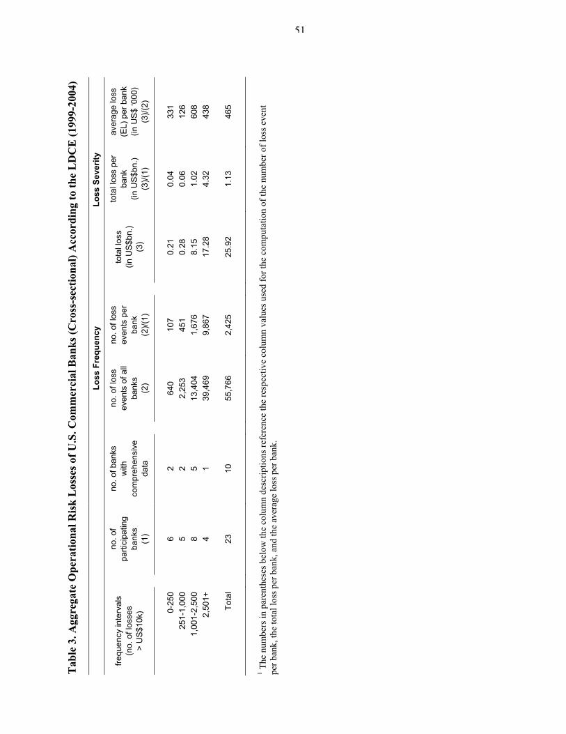
51

Tab

le 3

. Agg

rega

te O

pera

tiona

l Ris

k L

osse

s of U

.S. C

omm

erci

al B

anks

(Cro

ss-s

ectio

nal)

Acc

ordi

ng to

the

LD

CE

(199

9-20

04)

Loss

Fre

quen

cy

Lo

ss S

ever

ity

frequ

ency

inte

rval

s (n

o. o

f los

ses

>

US

$10k

)

no. o

f pa

rtici

patin

g ba

nks

(1)

no. o

f ban

ks

with

co

mpr

ehen

sive

da

ta

no. o

f los

s ev

ents

of a

ll ba

nks

(2)

no. o

f los

s ev

ents

per

ba

nk

(2)/(

1)

to

tal l

oss

(in

US

$bn.

) (3

)

tota

l los

s pe

r ba

nk

(in U

S$b

n.)

(3)/(

1)

aver

age

loss

(E

L) p

er b

ank

(in U

S$ ‘0

00)

(3)/(

2)

0-

250

6

2

640

107

0.

21

0.04

33

1 25

1-1,

000

5

2

2,25

3 45

1

0.28

0.

06

126

1,00

1-2,

500

8

5

13,4

04

1,67

6

8.15

1.

02

608

2,50

1+

4

1

39,4

69

9,86

7

17.2

8 4.

32

438

To

tal

23

10

55,7

66

2,42

5

25.9

2 1.

13

465

1 The

num

bers

in p

aren

thes

es b

elow

the

colu

mn

desc

riptio

ns re

fere

nce

the

resp

ectiv

e co

lum

n va

lues

use

d fo

r the

com

puta

tion

of th

e nu

mbe

r of l

oss e

vent

pe

r ban

k, th

e to

tal l

oss p

er b

ank,

and

the

aver

age

loss

per

ban

k.

52

Table 4. Descriptive Statistics of Simulated Daily Operational Risk Exposure Over a Five-Year Horizon (2000–2004), Calibrated to the LDCE (2004) Aggregate Statistics

(in US$ ’000).

Random sampling from GEV with shape parameter ξ

EV0 (ξ=0)

EV1 (ξ=0.85)

EV1 (ξ=1.0)

EV1 (ξ=1.15)

EV2 (ξ=-1.0)

mean1 670.2

median 437.4 39.5 61.0 126.5 471.8

maximum 5,957.1 524,400.0 575,708.3 415,569.5 1,932.6

Minimum2 0.0

std. dev. 685.4 8,390.3 8,740.2 7,078.8 591.8

coeff. of variance 1.0 12.5 13.0 10.6 0.9

JB statistic3 1.2E+04 2.0E+09 2.8E+09 1.1E+09 1.8E+03

p-value 0.00 0.00 0.00 0.00 0.00 obs. 9,996 Upper tail percentiles Median values of upper tail description

95.000 2,128.1 1,406.7 1,511.1 1,567.1 1,880.4 97.500 2,480.8 3,023.3 3,002.1 2,848.5 1,909.4 99.000 2,984.6 8,670.5 7,989.7 6,119.7 1,924.3 99.500 3,443.9 19,254.8 15,210.9 13,514.0 1,928.4 99.700 3,768.3 27,116.9 21,420.7 20,406.0 1,929.9 99.9004 4,337.8 83,774.7 78,948.6 75,444.5 1,931.9 99.950 4,623.8 157,275.1 161,078.4 178,388.7 1,932.3 99.970 4,905.0 199,161.7 183,839.1 184,046.2 1,932.5 99.990 5,350.6 404,739.5 441,892.0 277,889.9 1,932.6 99.999 5,896.4 512,433.9 562,326.7 401,801.6 1,932.6

1 The generic loss series are calibrated to the annual frequency and loss severity of operational risk events of U.S. banks based on the aggregate annual sample descriptives of LDCE between 2000 and 2004 (see shaded boxes in Table 2 above). The total number of observations reflects the sum of quarterly operational risk events from 2000 to 2004. Since the average number of reported operational risk events per bank in LDCE is insufficient for modeling purposes, we derive the number of annual operational risk events from scaling the actual loss frequency by a constant factor 2.91× so that the overall sample size reaches about 10,000 observations. The average loss severity is kept unchanged. We simulate operational risk losses on a quarterly basis, which allows us to control operational risk exposure for fundamental values, such gross income, in line with AMA. The sum of quarterly loss events does not sum up to the sample size due to rounding. 2 The left endpoint of the simulated loss distribution is rescaled to zero (in order to avoid negative quantile estimates), before the mean is calibrated to the annual expected loss in each simulation year over the five-year sample period (2000-04) covered by the LDCE sample statistics. 3 The Jarque-Bera (JB) test diagnostic indicates whether the null hypothesis of normally distributed residuals can be rejected. 4 AMA quantitative criteria for percentile level of reported unexpected operational risk losses (Basel Committee, 2004, 2005, and 2006b).

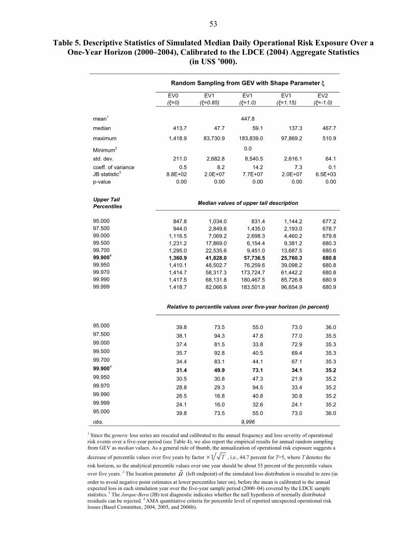
53

Table 5. Descriptive Statistics of Simulated Median Daily Operational Risk Exposure Over a One-Year Horizon (2000–2004), Calibrated to the LDCE (2004) Aggregate Statistics

(in US$ ’000).

Random Sampling from GEV with Shape Parameter ξ

EV0 (ξ=0)

EV1 (ξ=0.85)

EV1 (ξ=1.0)

EV1 (ξ=1.15)

EV2 (ξ=-1.0)

mean1 447.8

median 413.7 47.7 59.1 137.3 467.7

maximum 1,418.9 83,730.9 183,839.0 97,869.2 510.9

Minimum2 0.0

std. dev. 211.0 2,682.8 8,540.5 2,616.1 64.1 coeff. of variance 0.5 8.2 14.2 7.3 0.1 JB statistic3 8.8E+02 2.0E+07 7.7E+07 2.0E+07 6.5E+03 p-value 0.00 0.00 0.00 0.00 0.00

Upper Tail Percentiles Median values of upper tail description

95.000 847.8 1,034.0 831.4 1,144.2 677.2 97.500 944.0 2,849.6 1,435.0 2,193.0 678.7 99.000 1,116.5 7,069.2 2,698.3 4,460.2 679.8 99.500 1,231.2 17,869.0 6,154.4 9,381.2 680.3 99.700 1,295.0 22,535.6 9,451.0 13,687.5 680.6 99.9004 1,360.9 41,828.0 57,736.5 25,760.3 680.8 99.950 1,410.1 48,502.7 76,259.6 39,098.2 680.8 99.970 1,414.7 58,317.3 173,724.7 61,442.2 680.8 99.990 1,417.5 68,131.8 180,467.5 85,726.8 680.9 99.999 1,418.7 82,066.9 183,501.8 96,654.9 680.9

Relative to percentile values over five-year horizon (in percent)

95.000 39.8 73.5 55.0 73.0 36.0 97.500 38.1 94.3 47.8 77.0 35.5 99.000 37.4 81.5 33.8 72.9 35.3 99.500 35.7 92.8 40.5 69.4 35.3 99.700 34.4 83.1 44.1 67.1 35.3 99.9004 31.4 49.9 73.1 34.1 35.2 99.950 30.5 30.8 47.3 21.9 35.2 99.970 28.8 29.3 94.5 33.4 35.2 99.990 26.5 16.8 40.8 30.8 35.2 99.999 24.1 16.0 32.6 24.1 35.2 95.000 39.8 73.5 55.0 73.0 36.0 obs. 9,996

1 Since the generic loss series are rescaled and calibrated to the annual frequency and loss severity of operational risk events over a five-year period (see Table 4), we also report the empirical results for annual random sampling from GEV as median values. As a general rule of thumb, the annualization of operational risk exposure suggests a

decrease of percentile values over five years by factor 1 T× , i.e., 44.7 percent for T=5, where T denotes the risk horizon, so the analytical percentile values over one year should be about 55 percent of the percentile values over five years. 2 The location parameter μ% (left endpoint) of the simulated loss distribution is rescaled to zero (in order to avoid negative point estimates at lower percentiles later on), before the mean is calibrated to the annual expected loss in each simulation year over the five-year sample period (2000–04) covered by the LDCE sample statistics. 3 The Jarque-Bera (JB) test diagnostic indicates whether the null hypothesis of normally distributed residuals can be rejected. 4 AMA quantitative criteria for percentile level of reported unexpected operational risk losses (Basel Committee, 2004, 2005, and 2006b).

54

Tab

le 6

. Des

crip

tives

of S

imul

ated

Los

s Ser

ies b

ased

on

the

Agg

rega

te L

oss S

tatis

tics (

2000

–200

4), A

djus

ted

by

Qua

rter

ly V

alue

s of F

unda

men

tal B

ank

Dat

a (I

n Pe

rcen

t of T

otal

Ass

ets,

Gro

ss In

com

e, a

nd T

ier

1 C

apita

l), B

ank

1–41

Tota

l Ass

ets

(q

uart

erly

)

Gro

ss In

com

e (q

uart

erly

)

Tier

1 C

apita

l (q

uart

erly

)

Ban

k 1

(BoA

)1 B

ank

2 (J

PM

C)

Ban

k 3

(Wac

h)

Ban

k 4

(WaM

u)

B

ank

1 (B

oA)

Ban

k 2

(JP

MC

) B

ank

3 (W

ach)

B

ank

4 (W

aMu)

Ban

k 1

(BoA

) B

ank

2 (J

PM

C)

Ban

k 3

(Wac

h)

Ban

k 4

(WaM

u)

mea

n

0.00

009

0.00

009

0.00

019

0.00

024

0.

0053

1 0.

0063

7 0.

0124

4 0.

0165

5

0.00

445

0.00

160

0.00

31 0 0.

0031

0

med

ian

0.

0000

1 0.

0000

1 0.

0000

2 0.

0000

2

0.00

052

0.00

061

0.00

115

0.00

156

0.

0002

5 0.

0001

7 0.

0003 1

0.00

037

max

imum

0.09

324

0.08

793

0.17

419

0.21

162

5.

5205

8 5.

8432

7 11

.141

58

14.4

9674

3.74

334

1.55

050

2.74

85 1 3.

6320

7 m

inim

um

0.

0

0.0

0.

0

std.

dev

.

0.00

134

0.00

132

0.00

267

0.00

323

0.

0777

2 0.

0877

4 0.

1666

7 0.

2193

7

0.05

327

0.02

281

0.04

17 2 0.

0526

3 co

eff.

of v

aria

nce

1,

507.

8 1,

414.

4 1,

384.

6 1,

348.

6

1,46

2.5

1,37

7.6

1,33

9.5

1,32

5.9

1,

196.

4 1,

429.

5 1,

344.

7 1,

697.

3

sk

ewne

ss

52

.94

49.5

5 47

.54

47.2

8

52.5

8 47

.48

46.9

9 47

.06

44

.21

50.0

3 46

.41

54.2

8

kurto

sis

3,

284.

37

2,92

5.97

2,

712.

43

2,70

5.63

3,29

9.82

2,

729.

16

2,70

9.20

2,

699.

55

2,

644.

29

2,98

9.96

2,

631.

6 1 3,

344.

02

daily

obs

.2

9,99

6 1 W

e si

mul

ate

the

loss

dis

tribu

tion

from

GEV

(EV

1) w

ith sh

ape

para

met

er

1.0

ξ=

and

cal

ibra

te lo

sses

to th

e pu

blis

hed

aggr

egat

e lo

ss st

atis

tics o

f the

LD

CE

in 2

004.

2 The

ab

brev

iatio

ns d

enot

e th

e fo

llow

ing

bank

s: “

BoA

” (B

ank

of A

mer

ica)

, “JP

MC

” (J

.P. M

orga

n C

hase

), “W

ach”

(Wac

hovi

a) a

nd “

WaM

u” (W

ashi

ngto

n M

utua

l). 3 D

ue to

ro

undi

ng th

e lo

ss fr

eque

ncy

for e

ach

quar

ter o

ver t

he sa

mpl

e pe

riod

does

not

sum

up

to 1

0,00

0 ob

serv

atio

ns, w

hich

wer

e de

rived

from

the

scal

ing

the

num

ber o

f act

ual

obse

rvat

ions

per

ban

k ac

cord

ing

to th

e ag

greg

ate

loss

dis

tribu

tion

repo

rted

in d

e Fo

ntno

uvel

le (2

005)

on

the

resu

lts o

f the

LD

CE

in 2

004

for U

.S. c

omm

erci

al b

anks

.

55

Tab

le 7

. Des

crip

tives

of Q

uart

erly

Agg

rega

tes o

f Sim

ulat

ed L

oss S

erie

s bas

ed o

n th

e A

ggre

gate

Los

s Sta

tistic

s (20

00–2

004)

, A

djus

ted

by Q

uart

erly

Val

ues o

f Fun

dam

enta

l Ban

k D

ata

(In

Perc

ent o

f Tot

al A

sset

s, G

ross

Inco

me,

and

Tie

r 1

Cap

ital),

B

ank

1–41

Tota

l Ass

ets

(q

uart

erly

)

Gro

ss In

com

e (q

uart

erly

)

Tier

1 C

apita

l (q

uart

erly

)

Ban

k 1

(BoA

)2 B

ank

2 (J

PM

C)

Ban

k 3

(Wac

h)

Ban

k 4

(WaM

u)

B

ank

1 (B

oA)

Ban

k 2

(JP

MC

) B

ank

3 (W

ach)

B

ank

4 (W

aMu)

Ban

k 1

(BoA

) B

ank

2 (J

PM

C)

Ban

k 3

(Wac

h)

Ban

k 4

(WaM

u)

mea

n

0.04

442

0.04

652

0.09

639

0.11

975

2.

6560

0 3.

1674

9 6.

2332

4 8.

2432

1

2.22

550

0.79

762

1.55

077

1.54

982

med

ian

0.

0267

7 0.

0240

1 0.

0584

7 0.

0675

4

1.34

477

1.47

722

3.13

694

3.95

600

0.

6540

0 0.

4429

1 0.

9247

3 1.

1941

0 m

axim

um

0.

1295

1 0.

1455

8 0.

2683

3 0.

3379

9

7.66

798

11.0

6519

19

.074

28

25.9

4966

8.55

887

2.48

975

4.48

177

5.04

488

min

imum

0.00

417

0.00

422

0.01

057

0.01

336

0.

1960

7 0.

1927

2 0.

4061

0 0.

6693

4

0.06

174

0.07

254

0.16

827

0.23

068

std.

dev

.

0.04

016

0.04

372

0.08

807

0.10

998

2.

5588

4 3.

1966

2 6.

1976

4 8.

2532

4

2.92

630

0.75

002

1.45

634

1.24

770

coef

f. of

var

ianc

e

0.90

417

0.93

977

0.91

363

0.91

841

0.

9634

2 1.

0092

0 0.

9942

9 1.

0012

2

1.31

490

0.94

032

0.93

911

0.80

506

skew

ness

88.0

5 11

0.15

84

.94

86.1

5

90.3

9 12

0.11

96

.00

97.9

7

125.

36

111.

67

88.1

9 14

0.77

ku

rtosi

s

-62.

68

-4.5

2 -8

5.36

-8

6.84

-70.

13

47.0

4 -6

0.44

-5

7.80

-6.3

6 1.

44

-75.

98

210.

44

mea

n ob

s. p

er q

uarte

r

500

med

ian

obs.

per

qua

rter

50

9 qu

arte

rly o

bs.

20

1 W

e si

mul

ate

the

loss

dis

tribu

tion

of d

aily

loss

es fr

om G

EV (E

V1)

with

shap

e pa

ram

eter

1.

0ξ=

and

cal

ibra

te lo

sses

to th

e pu

blis

hed

aggr

egat

e lo

ss st

atis

tics o

f the

LD

CE

in

2004

(see

Tab

le 6

) bef

ore

aggr

egat

ing

to q

uarte

rly lo

ss v

alue

s. 2 T

he a

bbre

viat

ions

den

ote

the

follo

win

g ba

nks:

“B

oA”

(Ban

k of

Am

eric

a), “

JPM

C”

(J.P

. Mor

gan

Cha

se),

“Wac

h” (W

acho

via)

and

“W

aMu”

(Was

hing

ton

Mut

ual).

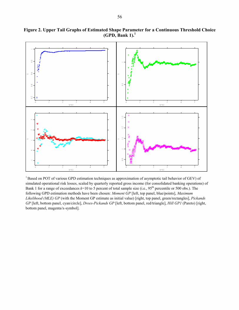
56

Figure 2. Upper Tail Graphs of Estimated Shape Parameter for a Continuous Threshold Choice

(GPD, Bank 1).1

1 Based on POT of various GPD estimation techniques as approximation of asymptotic tail behavior of GEV) of simulated operational risk losses, scaled by quarterly reported gross income (for consolidated banking operations) of Bank 1 for a range of exceedances k=10 to 5 percent of total sample size (i.e., 95th percentile or 500 obs.). The following GPD estimation methods have been chosen: Moment GP [left, top panel, blue/points], Maximum Likelihood (MLE) GP (with the Moment GP estimate as initial value) [right, top panel, green/rectangles], Pickands GP [left, bottom panel, cyan/circle], Drees-Pickands GP [left, bottom panel, red/triangle], Hill GP1 (Pareto) [right, bottom panel, magenta/x-symbol].

-

57

Table 8. Point Estimates of the Empirical, Normal and EVT-Based Distribution (Five-Year Risk Horizon, Scaled by Gross Income, Bank 1)1

VaR quantile estimates for different parametric specifications of tail behavior (in percent) EVT

GEV GPD Percenti

le emp. distr.

normal distr. exact

(LRS)

out-of-sample (LRS)

Moment Moment PL MLE MLE PL Pick-

ands DP Hill GP1

g-and-h distr.

95.000 0.01 13.31 0.01 0.01 0.02 0.03 0.02 0.02 0.03 0.03 0.01 0.0197.500 0.02 15.76 0.03 0.02 0.03 0.04 0.03 0.03 0.04 0.04 0.03 0.0299.000 0.06 18.61 0.08 0.06 0.06 0.09 0.06 0.06 0.06 0.06 0.06 0.0599.500 0.10 20.55 0.18 0.14 0.11 0.17 0.11 0.12 0.11 0.11 0.12 0.0899.700 0.17 21.89 0.33 0.25 0.17 0.28 0.18 0.20 0.17 0.17 0.19 0.1199.900 0.50 24.55 1.17 0.87 0.47 0.87 0.55 0.59 0.54 0.53 0.52 0.2199.950 1.09 26.10 2.58 1.91 0.89 1.81 1.12 1.22 1.16 1.15 0.99 0.3099.970 1.30 27.20 4.63 3.44 1.43 3.09 1.91 2.09 2.08 2.05 1.58 0.3999.990 4.03 29.44 16.30 12.09 4.05 9.86 5.98 6.65 7.33 7.20 4.36 0.6799.999 4.03 33.68 227.75 168.98 35.94 112.53 66.14 75.75 104.60 101.39 36.45 1.85

1 Point estimates of the empirical, normal and EVT-based distribution of a single i.i.d. operational risk loss event at the 95.0th and 97.5th (all in-sample) as well as 99.0th, 99.5th, 99.7th, 99.9th, 99.95th, 99.97th, 99.99th, and 99.999th (all out-of-sample) percentile over a five-year risk horizon. The percentile associated with the designated threshold value for GPD qualifies the classification of in- and out-of-sample estimation. We select k=100 (or 1 percent of the empirical quantile function) exceedances from 100 non-overlapping blocks of the total number of quasi-empirical losses of Bank 1 as i.i.d. maxima over a designated threshold. The following estimation methods for the generalized parametric distributions GEV, GPD, and g-and-h have been applied. We use the Linear Combination of Ratios of Spacings (LRS) method to estimate the μ[location], σ[scale], ξ[shape] parameters of GEV (Generalized Extreme Value). For GPD (Generalized Pareto Distribution), which approximates GEV for very high levels of confidence via the Peak-over-Threshold (POT) method, we employ the Moment GP, Maximum Likelihood (MLE) GP (with the Moment GP estimate as initial value), Pickands GP, and Drees-Pickands (DP) GP estimation procedures to identify the μ[location], σ[scale], and ξ[shape] parameters. We selected k=100 (or 99.0 percent of the empirical quantile function) exceedances as conditional i.i.d. maxima over a designated threshold for exceedances. For the Moment GP and the MLE GP estimation, we also compute the quantile estimates under a different shape parameter ξ derived from Philips and Loretan (1990). For the g-and-h distribution, we complete a quantile estimation (Haoglin, 1985) based on 40 equidistant quantile increments (“percentile points” (Tukey, 1977)) from the 95.0th to the 100th percentile to determine the μ[location], σ[scale], g[skewness], and h[kurtosis] parameters. The point estimates at the 99.9th percentile are printed in boldface, because they reflect unexpected operational risk exposure at a percentile level set forth in the quantitative criteria of AMA for operational risk measurement under the New Basel Capital Accord (Basel Committee, 2004, 2005 and 2006b).

-

58

Table 9. Relative Deviation of Point Estimates of the Empirical, Normal and EVT-Based Distribution (Five-Year Risk Horizon, Scaled by Gross Income, Bank 1)1

Relative Deviation of Analytical Point Estimates (in percent)

EVT

GEV GPD

Percentile normal distr. exact

(LRS)

out-of-sample (LRS)

Moment Moment LP MLE MLE LP Pick-

ands DP Hill GP1

g-and-h distr.

95.000 114,682.8 9.6 -15.5 92.1 115.8 96.3 98.4 177.5 175.8 21.6 12.1

97.500 66,414.1 21.1 -8.5 37.5 68.4 36.6 39.4 64.5 64.0 12.8 0.899.000 29,966.8 33.9 0.1 0.56 40.20 0.56 4.33 0.55 0.55 0.56 -22.199.500 19,736.2 77.6 32.2 5.9 62.6 9.9 15.4 2.3 2.3 13.9 -25.099.700 13,068.9 99.0 48.0 3.0 69.1 10.9 17.6 2.2 2.1 13.7 -35.299.900 4,764.9 131.0 71.5 -7.79 73.16 9.30 17.78 6.31 5.76 3.20 -59.299.950 2,305.3 137.7 76.4 -18.2 66.5 3.5 12.6 7.1 6.2 -9.1 -72.399.970 1,998.7 257.3 165.1 10.7 138.7 47.0 61.1 60.3 58.4 22.0 -69.899.990 631.1 304.8 200.4 0.6 145.0 48.5 65.0 82.0 78.8 8.2 -83.399.999 736.4 5,556.6 4,096.9 792.7 2,694.9 1,542.7 1,781.5 2,497.9 2,418.2 805.2 -54.0

1 Relative deviation of analytical point estimates (see Table 8) from empirical quantile values at the 95.0th and 97.5th (all in-sample) as well as 99.0th, 99.5th, 99.7th, 99.9th, 99.95th, 99.97th, 99.99th, and 99.999th (all out-of-sample) percentile over a five-year risk horizon.

-

59

Table 10. Point Estimates of the Empirical, Normal and EVT-Based Distribution (One-Year Risk

Horizon, Scaled by Gross Income, Bank 1)1

VaR Quantile Estimates for Different Parametric Specifications of Tail Behavior (in percent)

EVT

GEV GPD

Year k

emp. distr.

normal distr. exact

(LRS)

out-of-sample (LRS)

Moment MLE Pick-ands DP Hill

GP1

g-and-h

distr.

2000 22 0.077 1.466 0.064 0.062 0.086 0.071 0.118 0.050 0.097 0.0172001 17 0.445 11.283 0.183 0.220 0.426 0.401 0.308 0.526 0.442 0.0632002 21 0.118 27.789 0.369 0.234 0.271 0.292 0.668 0.446 0.269 0.0762003 20 0.451 41.001 0.601 0.410 0.689 0.886 0.633 1.467 0.733 0.1192004 20 0.943 19.464 2.408 1.744 1.089 0.917 1.080 0.821 1.303 0.547

1 Point estimates of a single i.i.d. operational risk loss event of Bank 1 at the 99.9th (out-of-sample) percentile over a five-year risk horizon. We select k exceedances (~ 1 percent of the empirical quantile function, depending on the different sample size) each year over the entire sample time period of five years. The following estimation methods for the generalized parametric distributions GEV, GPD, and g-and-h have been applied. We use the Linear Combination of Ratios of Spacings (LRS) method to estimate the μ[location], σ[scale], ξ[shape] parameters of GEV (Generalized Extreme Value). For GPD (Generalized Pareto Distribution), which approximates GEV for very high levels of confidence via the Peak-over-Threshold (POT) method, we employ the Moment GP, Maximum Likelihood (MLE) GP (with the Moment GP estimate as initial value), Pickands GP, and Drees-Pickands (DP) GP estimation procedures to identify the μ[location], σ[scale], and ξ[shape] parameters. We selected exceedances as conditional i.i.d. maxima over a designated threshold. For the Moment GP and the MLE GP estimation, we also compute the quantile estimates under a different shape parameter ξ derived from Philips and Loretan (1990). For the g-and-h distribution, we complete a quantile estimation (Haoglin, 1985) based on 40 equidistant quantile increments (“percentile points” (Tukey, 1977)) from the 95.0th to the 100th percentile to determine the μ[location], σ[scale], g[skewness], and h[kurtosis] parameters. The point estimates at the 99.9th percentile are printed in boldface, because they reflect unexpected operational risk exposure at a percentile level set forth in the quantitative criteria of AMA for operational risk measurement under the New Basel Capital Accord (Basel Committee, 2004, 2005 and 2006b).

-

60

Table 11. Estimated Parameter Values from the Numerical Evaluation of Tail Behavior (Scaled by Gross Income, Bank 1–4)1

GEV GPD

Estimation method LRS Moment MLE Pickands DP Hill GP1 PL g-and-h

distr. Panel A: Bank 1 (BoA)

μ [location] 0.000003 0.000118 0.000141 0.000268 0.000265 - - 0.000005σ/β [scale] 0.000005 0.000006 0.000004 0.000002 0.000002 0.000006 - 0.000010ξ/α [shape] 1.145300 0.949170 1.044900 1.156000 1.150300 0.949170 0.945420 -

g [skewness] - - - - - - - 1.985492h [kurtosis] - - - - - - - -0.031397

Panel B: Bank 2 (JPMC)

μ [location] 0.000004 -0.000034 -0.000072 -0.000321 0.000048 - - 0.000006σ/β [scale] 0.000006 0.000009 0.000010 0.000027 0.000007 0.000007 - 0.000012ξ/α [shape] 1.161500 0.944180 0.935230 0.730800 1.003600 1.010200 0.946330 -

g [skewness] - - - - - - - 2.009666h [kurtosis] - - - - - - - -0.031397

Panel C: Bank 3 (Wachovia)

μ [location] 0.000007 0.000171 0.000129 0.000763 0.000776 - - 0.000011σ/β [scale] 0.000011 0.000017 0.000015 0.000002 0.000002 0.000019 - 0.000023ξ/α [shape] 1.183200 0.936000 0.981640 1.292800 1.305400 1.060900 0.956870 -

g [skewness] - - - - - - - 2.017893h [kurtosis] - - - - - - - -0.031855

Panel D: Bank 4 (WaMu) μ [location] 0.000009 0.000181 0.000089 0.000810 0.000934 - - 0.000016σ/β [scale] 0.000015 0.000025 0.000024 0.000007 0.000005 0.000028 - 0.000031ξ/α [shape] 1.183700 0.918090 0.949030 1.145000 1.220400 1.071400 0.975970 -

g [skewness] - - - - - - - 2.012979h [kurtosis] - - - - - - - -0.031855

1 The following estimation methods for the generalized parametric distributions GEV, GPD, and g-and-h have been applied. We use the Linear Combination of Ratios of Spacings (LRS) method to estimate the μ[location], σ[scale], ξ[shape] parameters of GEV (Generalized Extreme Value). For GPD (Generalized Pareto Distribution), which approximates GEV for very high levels of confidence via the Peak-over-Threshold (POT) method, we employ the Moment GP, Maximum Likelihood (MLE) GP (with the Moment GP estimate as initial value), Pickands GP, and Drees-Pickands (DP) GP estimation procedures to identify the μ[location], σ[scale], and ξ[shape] parameters. We selected k=100 (or 99.0 percent of the empirical quantile function) exceedances as conditional i.i.d. maxima over a designated threshold for exceedances. For the Moment GP and the MLE GP estimation, we also compute the quantile estimates under a different shape parameter ξ derived from Philips and Loretan (1990). For the g-and-h distribution, we complete a quantile estimation (Haoglin, 1985) based on 40 equidistant quantile increments (“percentile points” (Tukey, 1977)) from the 95.0th to the 100th percentile to determine the μ[location], σ[scale], g[skewness], and h[kurtosis] parameters. The domain of GPD includes all real numbers, positive and non-positive. Therefore, depending on how the distribution is fitted, GPD may assume negative values even if all the actual data used to fit the upper tail to the empirical quantile function are positive. The scale parameters σ and β conform to our nomenclature for GEV and GPD respectively. The tail index parameter α=1/ξ applies to the Hill GP1 (Pareto) and the Phillips-Loretan (PL) estimation procedures. The g and h parameters are used to calibrate the skewness and kurtosis of the fitted g-and-h distribution. Similar to GEV and GPD, the actual higher moments are infinite in our case. Note that the actual higher-order moments (skewness and kurtosis) take the following values (based on the general moments of the g-and-h distribution): 1.536E+06 and 1.473E+12 (Bank 1), 2.204E+06 and 2.927E+12 (Bank 2), 2.446E+06 and 3.534E+12 (Bank 3), 2.271E+06 and 3.071E+12 (Bank 4). Also note that the parameter estimates of this table also serve as consistency check as to whether the adjustment of the generic loss distribution by individual gross income distorts the extreme tail behavior of the simulated loss series based on shape parameter ξ=1.0.

-

61

Figure 3. Threshold-Quantile Surface of Operational Risk (GPD Estimates, Scaled by Gross Income, Bank 1)1

(a)

(b) (c)

(d) (e)

in-sample

out-of-sample

-

62

(f) (g)

(h) (I)

1 GPD point estimates [blue/dark grid] of a single i.i.d. operational risk loss event (simulated operational risk losses, scaled by quarterly reported gross income of Bank 1) for all (1,521) combinations of threshold levels [x-axis] and percentile levels of statistical confidence [z-axis] over a quantile range from 98.0 percent to 99.9 percent (at increments of 0.05 percent). The quantile function of quasi-empirical losses is displayed as a yellow, light grid. The cube is scaled to fit the grid of analytical GPD point estimates (except in (d), (g) and (h)). We use the Moment GP [first and second row, (a) and (b) (with and without color scale)], Maximum Likelihood (MLE) GP (with the Moment GP estimate as initial value) [second row, (c)], Pickands GP [third and fourth row, (d)-(e)], and Drees-Pickands (DP) GP [fourth row, (f)] estimation procedures to estimate all parameters μ[location], σ[scale], ξ[shape] of the Generalized Pareto Distribution for each threshold choice. For the Hill GP1 (Pareto) [fourth and fifth row, (g)-(i)] estimation, we derive estimates for σ[scale] and α[shape]. Since the threshold choice at the 99.9 percent quantile yields 10 exceedances for a total sample size of 9,996 observations, we can complete all GPD estimation procedures via the Peak-over-Threshold (POT) method. Figure (a) indicates the areas of in- and out-of-sample estimation.

-

63

Figure 4. Aggregate Sensitivity of Estimated Upper Tail to the Threshold Choice (Bank 1)1

-600%

-400%

-200%

0%

200%

400%

600%

800%

1000%

1200%

0.980

0.981

0.982

0.983

0.984

0.985

0.986

0.987

0.988

0.989

0.990

0.991

0.992

0.993

0.994

0.995

0.996

0.997

0.998

0.999

Threshold Quantile

Rel

. Dev

iati

on

-1500%

-500%

500%

1500%

2500%

3500%

75th quartilemaximummedianmean25th quartile (scaled to right axis)minimum (scaled to right axis)

1 The graph consolidates all point estimates of the upper tail from the 98.0th to the 99.9th percentile [z-axis] of the threshold-quantile surface (see Figure 3) over a threshold range between the 98.0th to the 99.9th percentile. Therefore, it shows the deviation of the aggregate statistics of upper tail point estimates from the actual values at each threshold choice. The median, mean, maximum, minimum and interquantile range (IQR) between the 25th and the 75th percentile of all point estimates in the upper tail are derived from the best estimation method (Moment) of quasi-empirical losses of Bank 1 (see Table 8).

-

64

Table 12. Summary Statistics of the Deviation of the Estimates from the Actual Upper Tail, Variable Threshold Choice (Absolute Values of Relative Deviation from Empirical Value,

Bank 1–4)1

Bank 1 (BoA)

Bank 2 (JPMC)

Bank 3 (Wachovia)

Bank 4 (WaMu)

Estimation method2 Moment Pickands Moment Moment Upper tail statistic mean median mean median mean median mean median actual values 0.09 0.06 0.11 0.07 0.22 0.14 0.30 0.18

Deviation of point estimates (in percent)

mean 38.45 68.90 183.81 306.00 34.94 62.99 48.47 89.56 median 5.47 4.15 9.27 3.36 6.46 2.58 8.58 3.89 std. dev. 95.39 165.35 808.83 1,369.38 104.77 197.56 139.46 264.15 minimum 1.53 0.17 0.09 0.15 0.40 0.00 2.75 0.22

at percentile 98.90 98.00 98.55 98.10 99.45 98.30 98.95 98.75 maximum 491.47 772.49 4,967.95 8,379.85 633.78 1174.25 654.29 1,225.51

at percentile 99.90 99.90 99.85 99.85 99.85 99.85 99.90 99.90 correl. ρ(deviation, threshold) 0.54 0.61 0.35 0.35 0.43 0.46 0.47 0.51 skewness 3.63 3.08 5.77 5.72 5.23 5.02 3.96 3.86 kurtosis 14.29 9.74 34.51 34.05 29.72 27.73 15.16 14.56

obs. 39 1 The table shows the descriptive statistics of the mean and median point estimates over the upper tail (98.0th-99.9th percentile) for a variable threshold choice (98.0th–99.9th percentile) (see Figure 4). We also report the correlation coefficient of the percentile level and the deviation of the estimated from the actual mean/median of the upper tail. 2 The best estimation method of quasi-empirical losses for the ex ante threshold choice determines the estimation method for the optimization of the threshold choice though sensitivity analysis (see Table 8).

-

65

Figure 5. Aggregate Sensitivity of Individual Point Estimates to the Percentile Level of Statistical Confidence (Bank 1)1

-70%

-50%

-30%

-10%

10%

30%

50%

0.980

0.981

0.982

0.983

0.984

0.985

0.986

0.987

0.988

0.989

0.990

0.991

0.992

0.993

0.994

0.995

0.996

0.997

0.998

0.999

Percentile

Rel

ativ

e d

ev.

-1500%

-1000%

-500%

0%

500%

1000%

1500%

25th quartile75th quartilemedianmeanmaximum (scaled to right axis)minimum (scaled toright axis)

1 The graph consolidates the distribution of point estimates from the 98.0th to the 99.9th percentile [x-axis] of the threshold-quantile surface at percentile levels of 98.0 percent statistical confidence and above (see Figure 3). Thus, it shows the dispersion of point estimates around the empirical quantile value over the threshold range (98.0th-99.9th percentile) at each percentile level. The median, mean, maximum, minimum and interquantile range (IQR) between the 25th and the 75th percentile of all point estimates in the upper tail are derived from the best estimation method (Moment) of quasi-empirical losses of Bank 1 (see Table 8).

66

Tab

le 1

3. S

umm

ary

Stat

istic

s of t

he D

evia

tion

of P

oint

Est

imat

es A

roun

d th

e A

ctua

l Upp

er T

ail Q

uant

ile V

alue

, Var

iabl

e Pe

rcen

tile

Val

ue (A

bsol

ute

Val

ues o

f Rel

ativ

e D

evia

tion

from

Em

piri

cal V

alue

, Ban

k 1–

4)1

B

ank

1 (B

oA)

B

ank

2 (J

PMC

)

Ban

k 3

(Wac

hovi

a)

B

ank

4 (W

aMu)

Est

imat

ion

met

hod2

Mom

ent

Pick

ands

M

omen

t

M

omen

t

ab

s. d

ev. o

f es

timat

e

abs.

dev

. of

estim

ate

ab

s. d

ev. o

f es

timat

e

abs.

dev

. of

estim

ate

Poi

nt e

stim

ate

stat

istic

ov

er th

resh

old

rang

e m

ean

med

ian

actu

al

valu

e

(in

perc

ent)

m

ean

med

ian

actu

al v

alue

(in

per

cent

)

mea

n m

edia

n

actu

al

valu

e (in

pe

rcen

t)

mea

n m

edia

n

actu

al

valu

e (in

pe

rcen

t)

D

evia

tion

of p

oint

est

imat

es (i

n pe

rcen

t)

Upp

er ta

il st

atis

tics

M

ean

29.1

0 3.

99

0.10

286.

45

3.91

0.

11

60

.92

3.17

0.

23

87

.60

3.40

0.

31

Med

ian

26.6

4 2.

95

0.06

227.

15

2.73

0.

07

57

.17

2.26

0.

14

81

.88

1.92

0.

18

std.

Dev

. 19

.23

3.70

0.

11

24

8.66

3.

85

0.12

44.8

3 3.

67

0.26

63.9

7 4.

08

0.34

M

inim

um

1.11

0.

29

0.03

3.31

0.

17

0.03

1.32

0.

00

0.07

0.17

0.

00

0.10

at

Per

cent

ile

99.4

5 98

.30

98.0

0

99.8

5 98

.75

98.0

0

99.6

0 98

.95

98.0

0

99.6

5 98

.35

98.0

0 M

axim

um

66.5

5 15

.68

0.50

791.

07

20.1

1 0.

59

14

1.67

18

.93

1.32

202.

39

19.8

1 1.

75

at P

erce

ntile

98

.00

99.8

5 99

.90

98

.00

99.9

0 99

.90

98

.00

99.7

0 99

.90

98

.00

99.7

0 99

.90

corre

l. ρ (

devi

atio

n, p

erce

ntile

) -0

.95

0.72

-

-0

.97

-0.0

8 -

-0

.99

0.55

-

-0

.99

0.58

-

Ske

wne

ss

0.38

1.

69

2.76

0.59

2.

14

2.62

0.24

2.

71

2.97

0.21

2.

27

2.92

K

urto

sis

-1.0

3 2.

45

7.67

-0.9

4 7.

16

7.07

-1.2

4 8.

89

9.58

-1.2

3 6.

26

9.22

ob

s.

39

1 The

tabl

e sh

ows t

he d

escr

iptiv

e st

atis

tics o

f the

mea

n an

d m

edia

n po

int e

stim

ates

ove

r the

thre

shol

d ra

nge

(98.

0th-9

9.9th

per

cent

ile) a

t per

cent

ile le

vels

of 9

8.0

perc

ent s

tatis

tical

con

fiden

ce a

nd a

bove

(see

Fig

ure

5). W

e al

so re

port

the

corr

elat

ion

coef

ficie

nt o

f the

thre

shol

d qu

antil

e an

d th

e de

viat

ion

of th

e es

timat

ed

mea

n/m

edia

n po

int e

stim

ate

from

the

actu

al q

uant

ile v

alue

. 2 The

bes

t est

imat

ion

met

hod

of q

uasi

-em

piric

al lo

sses

for t

he e

x an

te th

resh

old

choi

ce d

eter

min

es th

e es

timat

ion

met

hod

for t

he o

ptim

izat

ion

of th

e th

resh

old

choi

ce th

ough

sens

itivi

ty a

naly

sis (

see

Tabl

e 8)

.

-

67

Figure 6. Single Point Estimate Graphs of a GPD-Fitted Distribution with a Variable Threshold Choice (Bank 1)1

1 The graphs show the threshold sensitivity at the 99.85th [left panel], 99.90th [center panel], and 99.95th percentile [right panel] of a GPD fitted distribution with a variable threshold choice (97.0th to the 99.5th percentile). The following GPD estimation methods have been chosen: Moment GP [blue/points], Maximum Likelihood (MLE) GP (with the Moment GP estimate as initial value) [green/rectangles], Pickands GP [cyan/circle], Drees-Pickands GP [red/triangle], Hill GP1 (Pareto) [magenta/x-symbol]. For the Moment GP [blue/small points] and the MLE GP [green/small rectangles] estimation, we also compute point estimates under a different shape parameter ξ derived from Philips and Loretan (PL) (1990).

-

68

Figure 7. Relative Deviation of Point Estimates (Point Estimate Residuals) from the Actual

Quantile Value Based on a Fixed Percentile Level (Bank 1)1

-50%

-30%

-10%

10%

30%

50%

70%

90%

110%

0.970

0.971

0.972

0.974

0.975

0.976

0.977

0.978

0.980

0.981

0.982

0.983

0.984

0.986

0.987

0.988

0.989

0.990

0.992

0.993

0.994

Threshold Quantile

Rel

. Dev

iati

on

-100%

-50%

0%

50%

100%

150%

200%

250%

300%

350%

median of all estimation methods

Drees Pickands (DP)

Pickands

MLE

Moment

Hill GP1 (scales to right axis)

Moment with PL shape parameter (scaled to right axis)

MLE with PL shape parameter (scaled to right axis)

1 The graph shows the deviations at the 99.9th percentile for a variable threshold choice (97.0th to the 99.5th percentile) (see Figure 6). The following GPD estimation methods have been chosen: Moment GP [blue/points], Maximum Likelihood (MLE) GP (with the Moment GP estimate as initial value) [green/rectangles], Pickands GP [cyan/circle], Drees-Pickands GP [red/triangle], Hill GP1 (Pareto) [magenta/x-symbol]. For the Moment GP [black/empty circle] and the MLE GP [grey/empty rectangle] estimation, we also compute point estimates under a different shape parameter ξ derived from Philips and Loretan (PL) (1990).

-

69

Figure 8. Single Point Estimate Graphs of a GPD-Fitted Distribution with a Variable Percentile Level (Bank 1)1

1 The graphs show the upper tail sensitivity at the 99.85th [left panel], 99.90th [center panel], and 99.95th threshold quantile [right panel] of a GPD fitted distribution with a variable percentile (97.0th to the 99.5th percentile). The following GPD estimation methods have been chosen: Moment GP [blue/points], Maximum Likelihood (MLE) GP (with the Moment GP estimate as initial value) [green/rectangles], Pickands GP [cyan/circle], Drees-Pickands GP [red/triangle], Hill GP1 (Pareto) [magenta/x-symbol]. For the Moment GP [blue/small points] and the MLE GP [green/small rectangles] estimation, we also compute point estimates under a different shape parameter ξ derived from Philips and Loretan (PL) (1990).

-

70

Figure 9. Relative Deviation of Point Estimates (Point Estimate Residuals) From the Actual Quantile Value Based on a Fixed Threshold Quantile (Bank 1)1

-40%

-20%

0%

20%

40%

60%

80%

100%

120%

140%

160%

180%

200%

0.975

0.976

0.977

0.978

0.979

0.980

0.981

0.982

0.983

0.984

0.985

0.986

0.987

0.988

0.989

0.990

0.991

0.992

0.993

0.994

0.995

0.996

0.997

0.998

0.999

Percentile

Rel

. Dev

iati

on

0%

50%

100%

150%

200%

250%

300%

350%

400%

450%

median of all estimation methodsDrees Pickands (DP)PickandsMLEMomentMoment with PL shape parameterMLE with PL shape parameterHill GP1 (scaled to right axis)

1 The graph shows the deviations at the 99.9th threshold quantile for a variable percentile level (97.0th to the 99.5th percentile) (see Figure 8). The following GPD estimation methods have been chosen: Moment GP [blue/points], Maximum Likelihood (MLE) GP (with the Moment GP estimate as initial value) [green/rectangles], Pickands GP [cyan/circle], Drees-Pickands GP [red/triangle], Hill GP1 (Pareto) [magenta/x-symbol]. For the Moment GP [black/empty circle] and the MLE GP [grey/empty rectangle] estimation, we also compute point estimates under a different shape parameter ξ derived from Philips and Loretan (PL) (1990).

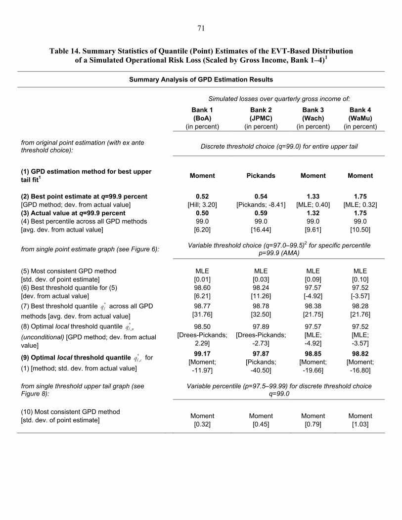
71

Table 14. Summary Statistics of Quantile (Point) Estimates of the EVT-Based Distribution of a Simulated Operational Risk Loss (Scaled by Gross Income, Bank 1–4)1

Summary Analysis of GPD Estimation Results

Simulated losses over quarterly gross income of:

Bank 1 (BoA)

(in percent)

Bank 2 (JPMC)

(in percent)

Bank 3 (Wach)

(in percent)

Bank 4 (WaMu)

(in percent)

from original point estimation (with ex ante threshold choice):

Discrete threshold choice (q=99.0) for entire upper tail

(1) GPD estimation method for best upper tail fit1 Moment Pickands Moment Moment

(2) Best point estimate at q=99.9 percent [GPD method; dev. from actual value] 0.52

[Hill; 3.20] 0.54

[Pickands; -8.41] 1.33

[MLE; 0.40] 1.75

[MLE; 0.32] (3) Actual value at q=99.9 percent 0.50 0.59 1.32 1.75 (4) Best percentile across all GPD methods [avg. dev. from actual value] 99.0

[6.20] 99.0

[16.44] 99.0 [9.61]

99.0 [10.50]

from single point estimate graph (see Figure 6): Variable threshold choice (q=97.0–99.5)2 for specific percentile p=99.9 (AMA)

(5) Most consistent GPD method [std. dev. of point estimate] MLE

[0.01] MLE [0.03]

MLE [0.09]

MLE [0.10]

(6) Best threshold quantile for (5) [dev. from actual value] 98.60

[6.21] 98.24 [11.26]

97.57 [-4.92]

97.52 [-3.57]

(7) Best threshold quantile *lq across all GPD

methods [avg. dev. from actual value] 98.77

[31.76] 98.78 [32.50]

98.38 [21.75]

98.28 [21.76]

(8) Optimal local threshold quantile *,l uq

(unconditional) [GPD method; dev. from actual value]

98.50

[Drees-Pickands; 2.29]

97.89 [Drees-Pickands;

-2.73]

97.57 [MLE; -4.92]

97.52 [MLE; -3.57]

(9) Optimal local threshold quantile *,l cq for

(1) [method; std. dev. from actual value]

99.17 [Moment; -11.97]

97.87 [Pickands;

-40.50]

98.85 [Moment; -19.66]

98.82 [Moment; -16.80]

from single threshold upper tail graph (see Figure 8): Variable percentile (p=97.5–99.99) for discrete threshold choice

q=99.0 (10) Most consistent GPD method [std. dev. of point estimate]

Moment [0.32]

Moment [0.45]

Moment [0.79]

Moment [1.03]

72

1 The GPD (Generalized Pareto Distribution) approximation of GEV via the Peak-over-Threshold (POT) method has been estimated with Moment GP, Maximum Likelihood (MLE) GP (with the Moment GP estimate as initial value), Pickands GP, Drees-Pickands (DP) GP, and the Hill GP1 estimation procedures. 2 We confine the variable threshold choice to a quantile range from 97.0 to 99.5 percent in order to avoid high parameter uncertainty for an overly restrictive designation of exceedances. 3 Tables 12 and 13 report only results for the estimation method that provides the best original upper tail fit (see Tables 8–10). 4 Since the large sample size of quasi-empirical losses allows for a high threshold choice to support the estimation of conditional mean excess, we choose a more restrictive range of threshold quantiles (98.0–99.9 percent) with smaller intervals for the global optimization of the threshold choice.

Summary Analysis of GPD Estimation Results (continued)

Simulated losses over quarterly gross income of:

Bank 1 (BoA)

(in percent)

Bank 2 (JPMC)

(in percent)

Bank 3 (Wach)

(in percent)

Bank 4 (WaMu)

(in percent)

from single threshold upper tail graph (see Figure 8): Variable percentile (p=97.5–99.99) for discrete threshold choice

q=99.0 (11) Best percentile for (10)3 [dev. from actual value] 99.92

[-38.89] 99.91

[-30.44] 99.92

[-35.20] 99.94

[-32.39] (12) Best percentile *

lp across all GPD methods [avg. dev. from actual value]

99.92 [-0.08]

99.91 [-12.59]

99.92 [2.60]

99.94 [12.75]

(13) Optimal local percentile *,l up

(unconditional)3 [GPD method; dev. from actual value]

99.92

[MLE PL; -14.04]

99.91 [MLE PL; -

1.31]

99.82 [Pickands; -

13.96]

99.82 [Pickands; -

13.49]

(14) Optimal local percentile *,l cp for (1)

[method; std. dev. from actual value]

99.92 [Moment; -

38.89]

99.91 [Pickands; -

26.48]

99.92 [Moment; -

35.20]

99.94 [Moment; -

32.39]

from Tables 11 & 12 (thresh.-quantile surface): Variable threshold choice (q=98.0–99.9)4 for entire upper tail(p=98.0-99.9)

(15) Optimal global threshold quantile *,g cq for

(1)2 [method; abs. dev. of median estimate]

98.00 [Moment;

2.95]

98.10 [Pickands;

0.15]

98.30 [Moment;

0.00]

98.75 [Moment;

0.22]

(16) Optimal global percentile *,g cp for (1)

[method; abs. dev. of median estimate]

98.30 [Moment;

0.29]

98.75 [Pickands;

0.17]

98.95 [Moment;

0.00]

98.35 [Moment;

0.00]