
PrMet Ch20 Numerical Weather Prediction (NWP) · 746 chaPter 20 • Numerical Weather PredictioN...
48
745 Copyright © 2015 by Roland Stull. Practical Meteorology: An Algebra-based Survey of Atmospheric Science. 20 NUMERICAL WEATHER PREDICTION (NWP) Most weather forecasts are made by computer, and some of these forecasts are further enhanced by humans. Computers can keep track of myriad complex nonlinear interactions among winds, tem- perature, and moisture at thousands of locations and altitudes around the world — an impossible task for humans. Also, data observation, collection, analysis, display and dissemination are mostly au- tomated. Fig. 20.1 shows an automated forecast. Produced by computer, this meteogram (graph of weather vs. time for one location) is easier for non-meteorologists to interpret than weather maps. But to produce such forecasts, the equations describing the atmosphere must first be solved. Contents Scientific Basis of Forecasting 746 The Equations of Motion 746 Approximate Solutions 749 Dynamics, Physics and Numerics 749 Models 751 Grid Points 752 Nested and Variable Grids 752 Staggered Grids 753 Finite-Difference Equations 754 Notation 754 Approximations to Spatial Gradients 754 Grid Computation Rules 756 Time Differencing 757 Discretized Equations of Motion 758 Numerical Errors & Instability 759 Round-off Error 759 Truncation Error 760 Numerical Instability 760 The Numerical Forecast Process 762 Balanced Mass and Flow Fields 763 Data Assimilation and Analysis 765 Forecast 768 Case Study: 22-25 Feb 1994 768 Post-processing 770 Nonlinear Dynamics And Chaos 773 Predictability 773 Lorenz Strange Attractor 773 Ensemble Forecasts 776 Probabilistic Forecasts 777 Forecast Quality & Verification 777 Continuous Variables 777 Binary / Categorical Events 780 Probabilistic Forecasts 782 Cost / Loss Decision Models 784 Review 786 Homework Exercises 787 Broaden Knowledge & Comprehension 787 Apply 788 Evaluate & Analyze 790 Synthesize 791 “Practical Meteorology: An Algebra-based Survey of Atmospheric Science” by Roland Stull is licensed under a Creative Commons Attribution-NonCom- mercial-ShareAlike 4.0 International License. View this license at http://creativecommons.org/licenses/by-nc-sa/4.0/ . This work is available at http://www.eos.ubc.ca/books/Practical_Meteorology/ . Figure 20.1 Two-day weather forecast for Jackson, Mississippi USA, plot- ted as a meteogram (time series), based on initial conditions observed at 12 UTC on 31 Oct 2015. (a) Temperature & dew- point (°F), (b) winds, (c) humidity, precipitation, cloud-cover, (d) rainfall amounts, (e) thunderstorm likelihood, (f) probability of precipitation > 0.25 inch. Produced by US NWS. (a) (b) (c) (d) (e) (f) Local Time 00 06 12 18 00 06 12 31 Oct | 1 Nov 2015 | 2 Nov
Transcript of PrMet Ch20 Numerical Weather Prediction (NWP) · 746 chaPter 20 • Numerical Weather PredictioN...

745
Copyright © 2015 by Roland Stull. Practical Meteorology: An Algebra-based Survey of Atmospheric Science.
20 Numerical Weather PredictioN (NWP)
Most weather forecasts are made by computer, and some of these forecasts are further enhanced by humans. Computers can keep track of myriad complex nonlinear interactions among winds, tem-perature, and moisture at thousands of locations and altitudes around the world — an impossible task for humans. Also, data observation, collection, analysis, display and dissemination are mostly au-tomated. Fig. 20.1 shows an automated forecast. Produced by computer, this meteogram (graph of weather vs. time for one location) is easier for non-meteorologists to interpret than weather maps. But to produce such forecasts, the equations describing the atmosphere must first be solved.
contents
Scientific Basis of Forecasting 746The Equations of Motion 746Approximate Solutions 749Dynamics, Physics and Numerics 749Models 751
Grid Points 752Nested and Variable Grids 752Staggered Grids 753
Finite-Difference Equations 754Notation 754Approximations to Spatial Gradients 754Grid Computation Rules 756Time Differencing 757Discretized Equations of Motion 758
Numerical Errors & Instability 759Round-off Error 759Truncation Error 760Numerical Instability 760
The Numerical Forecast Process 762Balanced Mass and Flow Fields 763Data Assimilation and Analysis 765Forecast 768Case Study: 22-25 Feb 1994 768Post-processing 770
Nonlinear Dynamics And Chaos 773Predictability 773Lorenz Strange Attractor 773Ensemble Forecasts 776Probabilistic Forecasts 777
Forecast Quality & Verification 777Continuous Variables 777Binary / Categorical Events 780Probabilistic Forecasts 782Cost / Loss Decision Models 784
Review 786
Homework Exercises 787Broaden Knowledge & Comprehension 787Apply 788Evaluate & Analyze 790Synthesize 791
“Practical Meteorology: An Algebra-based Survey of Atmospheric Science” by Roland Stull is licensed under a Creative Commons Attribution-NonCom-
mercial-ShareAlike 4.0 International License. View this license at http://creativecommons.org/licenses/by-nc-sa/4.0/ . This work is available at http://www.eos.ubc.ca/books/Practical_Meteorology/ .
Figure 20.1Two-day weather forecast for Jackson, Mississippi USA, plot-ted as a meteogram (time series), based on initial conditions observed at 12 UTC on 31 Oct 2015. (a) Temperature & dew-point (°F), (b) winds, (c) humidity, precipitation, cloud-cover, (d) rainfall amounts, (e) thunderstorm likelihood, (f) probability of precipitation > 0.25 inch. Produced by US NWS.
(a)
(b)
(c)
(d)
(e)
(f)
Local Time 00 06 12 18 00 06 1231 Oct | 1 Nov 2015 | 2 Nov

746 chaPter 20 • Numerical Weather PredictioN (NWP)
Scientific BaSiS of forecaSting
the equations of Motion Numerical weather forecasts are made by solv-ing Eulerian equations for U, V, W, T, rT, ρ and P. From the Forces & Winds chapter are forecast equations for the three wind components (U, V, W) (modified from eqs. 10.23a & b, and eq. 10.59):
(20.1)
∆∆
= − ∆∆
− ∆∆
− ∆∆
− ∆∆
+
Ut
UUx
VUy
WUz
Px
f Vc
· · 1ρ
−−∆ ( )
∆
F U
zz turb
(20.2)
∆∆
= − ∆∆
− ∆∆
− ∆∆
− ∆∆
−
Vt
UVx
VVy
WVz
Py
f Uc
· ·1ρ
∆ ( )
∆−
F V
zz turb
(20.3)∆∆
∆∆
∆∆
∆∆
Wt
UWx
VWy
WWz
Pz T
v p ve
ve
= − − −
− ′ +−1
ρθ θ∆
∆· gg
F W
zz turb−
∆ ( )
∆
From the Heat Budgets chapter is a forecast equa-tion for temperature T (modified from eq. 3.51):
(20.4)∆∆
·
∆
Tt
UTx
VTy
WTz
C
d
p
= − ∆∆
− ∆∆
− ∆∆
+
−
Γ
1ρ
Fzz rad v
p
condensing z turb
zLC
r
t
F
z
*
∆
∆
∆
∆ ( )
∆+ −
θ
From the Water Vapor chapter is a forecast equa-tion (4.44) for total-water mixing ratio rT in the air:
(20.5)
∆∆
∆∆
∆
rt
Urx
Vry
Wrz
Prz
T T T T
L
d
= − ∆∆
− ∆∆
− ∆∆
+ −ρρ
FF r
zz turb T( )
∆
From the Forces & Winds chapter is the continu-ity equation (10.60) to forecast air density ρ: (20.6)
∆∆ρ ρ ρ ρ ρt
Ux
Vy
Wz
Ux
Vy
Wz
= − ∆∆
− ∆∆
− ∆∆
− ∆∆
+ ∆∆
+ ∆∆
For pressure P, use the equation of state (ideal gas law) from Chapter 1 (eq. 1.23):
P Td v= ℜρ· · (20.7)
info • alternative Vertical coordinate
Eqs. (20.1-20.7) use z as a vertical coordinate, where z is height above mean sea level. But local terrain ele-vations can be higher than sea level. The atmosphere does not exist underground; thus, it makes no sense to solve the meteorological equations of motion at heights below ground level. To avoid this problem, define a terrain-follow-ing coordinate σ (sigma). One definition for σ is based on the hydrostatic pressure Pref(z) at any height z relative to the hydrostatic pressure difference be-tween the earth’s surface (Pref bottom) and a fixed pres-sure (Pref top) representing the top of the atmosphere:
σ =
−−
P z P
P Pref ref top
ref bottom ref top
( )
Pref bottom varies in the horizontal due to terrain eleva-tion (see Fig. 20.A) and varies in space and time due to changing surface weather patterns (high- and low-pressure centers). The new vertical coordinate σ var-ies from 1 at the earth’s surface to 0 at the top of the domain. The figure below shows how this sigma coor-dinate varies over a mountain. hybrid coordi-nates (Fig. 20.5) are ones that are terrain following near the ground, but constant pressure aloft. If σ is used as a vertical coordinate, then (U, V) are defined as winds along a σ surface. The vertical advection term in eq. (20.1) changes from W·∆U/∆z to · ·∆ /∆σ σU , where sigma dot is analogous to a verti-
cal velocity, but in sigma coordinates. Similar chang-es must be made to most of the terms in the equations of motion, which can be numerically solved within the domain of 0 ≤ σ ≤ 1.
Figure 20.a. Vertical cross section through the atmosphere (white) and earth (black). White numbers represent surface air pressure at the weather stations shown by the grey dots. For the equation above, Pref bottom = 70 kPa at the mountain top, which differs from Pref bottom = 90 kPa in the valley.
Although sigma coordinates avoid the problem of coordinates that go underground, they create prob-lems for advection calculations due to small differ-ences between large terms. To reduce this problem, stair-step terrain-following coordinates have been devised — known as eta coordinates (η).

r. Stull • Practical meteorology 747
In these seven equations: fc is Coriolis parameter, P’ is the deviation of pressure from its hydrostatic value, θvp and θve are virtual potential temperatures of the air parcel and the surrounding environment, Tve is virtual temperature of the environment, |g| = 9.8 m s–2 is the magnitude of gravitational accelera-tion, Γd = 9.8 K km–1 is the dry adiabatic lapse rate, F*z rad is net radiative flux, Lv ≈ 2.5x10⁶ J kg–1 is the latent heat of vaporization, Cp ≈ 1004 J·kg–1·K–1 is the specific heat of air at constant pressure, ∆rcondensing is the increase in liquid-water mixing ratio associ-ated with water vapor that is condensing, ρL ≈ 1000 kg·m–3 and ρd are the densities of liquid water and dry air, Pr is precipitation rate (m s–1) of water ac-cumulation in a rain gauge at any height z, ℜd = 287 J·kg–1·K–1 is the gas constant for dry air, and Tv is the virtual temperature. For more details, see the chap-ters cited with those equations. Notice the similarities in eqs. (20.1 - 20.6). All have a tendency term (rate of change with time) on the left. All have advection as the first 3 terms on the right. Eqs. (20.1 - 20.5) include a turbulence flux divergence term on the right. The other terms describe the special forcings that apply to individ-ual variables. Sometimes the hydrostatic equation (Chapter 1, eq. 1.25b) is also included in the set of forecast equations:
∆
∆·
P
zg
ref = −ρ (20.8)
to serve as a reference state for the definition of P’ = P – Pref , as used in eq. (20.3). Equations (20.1) - (20.7) are the equations of mo-tion. They are also known as the primitive equa-tions, because they forecast fundamental (primi-tive) variables rather than derived variables such as vorticity. The first six equations are budget equa-tions, because they forecast how variables change in response to inputs and outputs. Namely, the first three equations describe momentum conserva-tion per unit mass of air. Eqs. (20.4 - 20.5) describe heat conservation and moisture conservation per unit mass of air. Eq. (20.6) describes mass con-servation. The first six equations are prognostic (i.e., fore-cast the change with time), and the seventh (the ideal gas law) is diagnostic (not a function of time). The third equation includes non-hydrostatic process-es, the fourth equation includes diabatic processes (non-adiabatic heating), and the sixth equation in-cludes compressible processes. These equations of motion are nonlinear, be-cause many of the terms in these equations consist of products of two or more dependent variables. Also, they are coupled equations, because each equation contains variables that are forecast or diagnosed
info • alternative Horizontal coord.
Spherical coordinates For the Cartesian coordinates used in eqs. (20.1-20.8), the coordinate axes are straight lines. However, on Earth we prefer to define x to follow the Earth’s curvature toward the East, and define y to follow the Earth’s curvature toward the North. If U and V are defined as velocities along these spherical coordi-nates, then add the following terms to the right side of the horizontal momentum equations (20.1-20.3):
+ − − [ ]U VR
U WR
Wo o
· · tan( ) ·· · ·cos( )
φφ2 Ω (20.1b)
− −U
RV W
Ro o
2 ·tan( ) ·φ (20.2b)
+ + + [ ]U VR
Uo
2 22· · ·cos( )Ω φ (20.3b)
where Ro ≈ 6371 km is the average Earth radius, ϕ is latitude, and Ω = 0.7292x10⁻⁴ s–1 is Earth’s rotation rate. The terms containing Ro are called the curvature terms. The terms in square brackets are small com-ponents of Coriolis force (see the INFO Box “Coriolis Force in 3-D” from the Forces & Winds chapter).
map Factors Suppose we pick (x, y) to represent horizontal co-ordinates on a map projection, such as shown in the INFO Box on the next page. Let (U, V) be the hori-zontal components of winds in these (x, y) directions. [Vertical velocity W applies unchanged in the z (up) direction.] One reason why meteorologists use such map projections is to avoid singularities, such as near the Earth’s poles where meridians converge. The equations of motion can be rewritten for any map projection. For example, eq. (20.1) can be written for a polar stereographic projection as:
∆∆
= − ∆∆
− ∆∆
− ∆∆
− +
Ut
m UUx
m VUy
WUz
m V m U
o o
x y
· ·
· ·2 ···
[ ]
· · ∆ (
VU W
RCor
m Px
f VF U
o
oc
z turb
− +
− ∆∆
+ −ρ
))
∆ z (20.1c)
where [Cor] is a 3-D Coriolis term, and the map fac-tors (m) are:
mL x y
R Loo
o=
++
=+ +1
1 2
2 2 2sin( )sin( ) · ·
φφand
m x R Lx o= /( · ) , m y R Ly o= /( · ) ,
where L Ro o= +·[ sin( )]1 φ , Ro ≈ 6371 km is the aver-age Earth radius, ϕ is latitude, and ϕo is the reference latitude for the map projection (see INFO Box). Thus, the equation has extra terms, and many of the terms are scaled by a map factor. Eqs. (20.2 - 20.6) have similar changes when cast on a map projection.

748 chaPter 20 • Numerical Weather PredictioN (NWP)
Sample application (§) Plot the given coordinates: (a) on a lat-lon grid, and (b) on a polar stereographic grid with ϕo = 60°.
Find the answer
Given: Latitudes (ϕ) & longitudes (λ) of N. America
Each column holds [ϕ(°) λ(°)]. λ is positive eastward
50 -12540 -12523 -11024 -11030 -11532 -11422 -10620 -1067 -809 -784 -760 -80 0 -4810 -6312 -73
9 -7611 -8415 -8415 -8822 -8722 -9018 -9118 -9622 -9827 -9730 -8528 -8325 -8126 -8030 -8235 -76
38 -7746 -6543 -6646 -6045 -6550 -6550 -6053 -5648 -5947 -5253 -5660 -6558 -6864 -7852 -7953 -83
55 -8258 -9568 -8270 -14073 -15765 -16858 -15853 -17060 -14660 -14050 -125
0 -900 90
0 00 180
0 -450 135 0 450 -135
0 00 100 200 300 etc.0 3500 360
Hint: In Excel, copy these numbers into 2 long columns: the first for latitudes and the second for longitudes. Leave blank rows in Excel corresponding to the blank lines in the table, to create discontinuous plotted lines.
(a) lat-lon grid:To save space,only the portionof the grid nearNorth Americais plotted. Fig. 20.B1.
(b) Polar Stereographic grid:Hint: In Excel, don’t forget to convert from (°) to (radians). To demonstrate the Excel calculation for the first coor-dinate (near Vancouver): ϕ = 50° , λ = –125° : L = (6371 km)·[1 + sin(60°·π/180°)] = 11,888 km. r = (11888 km)·tan[0.5·(90°– 50°)·π/180°] = 4327 km x = (4327 km)·cos(–125°·π/180°) = – 2482 km y = (4327 km)·sin(–125°·π/180°) = – 3545 km That point is circled on the maps above and below:
Fig. 20.B2
info • Map Projections
A map displays the 3-D Earth’s surface on a 2-D plane. On maps you can also: (1) create perpendicu-lar (x, y) coordinates; and (2) rewrite the equations of motion within these map coordinates. You can then solve these eqs. to make numerical weather forecasts. Create a map by projecting the spherical Earth on to a plane (stereographic projection), a cylinder (mercator projection), or a cone (lambert projec-tion), where the cylinder and cone can be “unrolled” after the projection to give a flat map. Although other map projections are possible, the 3 listed above are conformal, meaning that the angle between two intersecting curves on the Earth is equal to the angle between the same curves on the map. For stereographic projections, if the projector is at the North or South Pole, then the result is a polar stereographic projection (Fig. 20.C). For any lati-tude (ϕ) longitude (λ, positive eastward) coordinates on Earth, the corresponding (x, y) map coordinates are: x = r · cos(λ) , y = r · sin(λ) (F20.1)
r = L·tan[0.5·(90° – ϕ )] , L = Ro·[1+sin(ϕo)] (F20.2)
Ro = 6371 km = Earth’s radius, and ϕo is the latitude intersected by the projection plane. The Fig. below has ϕo = 60°, but often ϕo = 90° is used instead.
Fig. 20.c. Polar stereographic map projection.

r. Stull • Practical meteorology 749
from one or more of the other equations. Hence, all 7 equations must be solved together. Unfortunately, no one has yet succeeded in solv-ing the full governing equations analytically. An analytical solution is itself an algebraic equa-tion or number that can be applied at every loca-tion in the atmosphere. For example, the equation y2 + 2xy = 8x2 has an analytical solution y = 2x, which allows you to find y at any location x.
approximate Solutions To get around this difficulty of no analytical so-lution, three alternatives are used. One is to find an exact analytical solution to a simplified (approxi-mate) version of the governing equations. A second is to conceive a simplified physical model, for which exact equations can be solved. The third is to find an approximate numerical solution to the full gov-erning equations (the focus of this chapter). (1) An atmospheric example of the first method is the geostrophic wind, which is an exact solution to a highly simplified equation of motion. This is the case of steady-state (equilibrium) winds above the boundary layer where friction can be neglected, and for regions where the isobars are nearly straight. (2) Early numerical weather prediction (NWP) efforts used the 2nd method, because of the limited power of early computers. Rossby derived simplified equations by modeling the atmosphere as if it were one layer of water surrounding the Earth. Charney, von Neumann, and others extended this work and wrote a program for a one-layer baro-tropic atmosphere (Fig. 20.2a) for the ENIAC com-puter in 1950. These earliest programs forecasted only vorticity and geopotential height at 50 kPa. (3) Modern NWP uses the third method. Here, the full primitive equations are solved using fi-nite-difference approximations for full baroclinic scenarios (Fig. 20.2b), but only at discrete locations called grid points. Usually these grid points are at regularly-spaced intervals on a map, rather than at each city or town.
Dynamics, Physics and numerics If computers had infinite power, then we could: forecast the movement of every air molecule, fore-cast the growth of each snowflake and cloud droplet, precisely describe each turbulent eddy, consider at-mospheric interaction with each tree leaf and blade of grass, diagnose the absorption of radiation for an infinite number of infinitesimally fine spectral bands, account for every change in terrain elevation, and could even include the movement and activities of each human as they affect the atmosphere. But it might be a few years before we can do that. At pres-
Figure 20.2(a) Barotropic idealization, based on the standard atmosphere from Chapter 1. (b) Baroclinic example, based on data from the General Circulation chapter.
info • Barotropic vs. Baroclinic
In a barotropic atmosphere (Fig. 20.2a), the isobars (lines of equal pressure) do not cross the isopycnics (lines of equal density). This would occur for a situation where there are no variations of temperature in the horizontal. Hence, there could be no thermal-wind effect. In a baroclinic atmosphere (Fig. 20.2b), isobars can cross isopycnics. Horizontal temperature gra-dients contribute to the tilt of the isopycnics. These temperature gradients also cause changing horizon-tal pressure gradients with increasing altitude, ac-cording to the thermal-wind effect. The real atmosphere is baroclinic, due to differ-ential heating by the sun (see the General Circula-tion chapter). In a baroclinic atmosphere, potential energy associated with temperature gradients can be converted into the kinetic energy of winds.
750 chaPter 20 • Numerical Weather PredictioN (NWP)
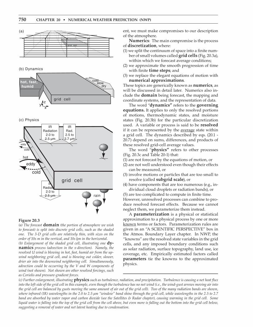
ent, we must make compromises to our description of the atmosphere. Numerics: The main compromise is the process of discretization, where: (1) we split the continuum of space into a finite num-
ber of small volumes called grid cells (Fig. 20.3a), within which we forecast average conditions;
(2) we approximate the smooth progression of time with finite time steps; and
(3) we replace the elegant equations of motion with numerical approximations.
These topics are generically known as numerics, as will be discussed in detail later. Numerics also in-clude the domain being forecast, the mapping and coordinate systems, and the representation of data. The word “dynamics” refers to the governing equations. It applies to only the resolved portions of motions, thermodynamic states, and moisture states (Fig. 20.3b) for the particular discretization used. A variable or process is said to be resolved if it can be represented by the average state within a grid cell. The dynamics described by eqs. (20.1 - 20.7) depend on sums, differences, and products of these resolved grid-cell average values. The word “physics” refers to other processes (Fig. 20.3c and Table 20-1) that:(1) are not forecast by the equations of motion, or (2) are not well understood even though their effects
can be measured, or (3) involve motions or particles that are too small to
resolve (called subgrid scale), or(4) have components that are too numerous (e.g., in-
dividual cloud droplets or radiation bands), or (5) are too complicated to compute in finite time. However, unresolved processes can combine to pro-duce resolved forecast effects. Because we cannot neglect them, we parameterize them instead. A parameterization is a physical or statistical approximation to a physical process by one or more known terms or factors. Parameterization rules are given in an “A SCIENTIFIC PERSPECTIVE” box in the Atmos. Boundary Layer chapter. In NWP, the “knowns” are the resolved state variables in the grid cells, and any imposed boundary conditions such as solar radiation, surface topography, land use, ice coverage, etc. Empirically estimated factors called parameters tie the knowns to the approximated physics.
Figure 20.3(a) The forecast domain (the portion of atmosphere we wish to forecast) is split into discrete grid cells, such as the shaded one. The 3-D grid cells are relatively thin, with sizes on the order of 10s m in the vertical, and 10s km in the horizontal. (b) Enlargement of the shaded grid cell, illustrating one dy-namics process (advection in the x-direction). Namely, the resolved U wind is blowing in hot, fast, humid air from the up-wind neighboring grid cell, and is blowing out colder, slower, drier air into the downwind neighboring cell. Simultaneously, advection could be occurring by the V and W components of wind (not shown). Not shown are other resolved forcings, such as Coriolis and pressure-gradient forces.(c) Further enlargement, illustrating physics such as turbulence, radiation, and precipitation. Turbulence is causing a net heat flux into the left side of the grid cell in this example, even though the turbulence has no net wind (i.e., the wind-gust arrows moving air into the grid cell are balanced by gusts moving the same amount of air out of the grid cell). Two of the many radiation bands are shown, where infrared (IR) wavelengths in the 2.0 to 2.5 µm “window” band shine through the grid cell, while wavelengths in the 2.5 to 2.7 band are absorbed by water vapor and carbon dioxide (see the Satellites & Radar chapter), causing warming in the grid cell. Some liquid water is falling into the top of the grid cell from the cell above, but even more is falling out the bottom into the grid cell below, suggesting a removal of water and net latent heating due to condensation.

r. Stull • Practical meteorology 751
Because parameterizations are only approxima-tions, no single parameterization is perfectly cor-rect. Different scientists might propose different pa-rameterizations for the same physical phenomenon. Different parameterizations might perform better for different weather situations.
Models The computer code that incorporates one partic-ular set of dynamical equations, numerical approxi-mations, and physical parameterizations is called a numerical model or NWP model. People devel-oping these extremely large sets of computer code are called modelers. It typically takes teams of modelers (meteorologists, physicists, chemists, and computer scientists) several years to develop a new numerical weather model. Different forecast centers develop different nu-merical models containing different dynamics, physics and numerics. These models are given names and acronyms, such as the Weather Research and Forecasting (WrF) model, the Global Environ-mental Multiscale (gem) model, or the Global Fore-cast System (gFS). Different models usually give slightly different forecasts.
table 20-1. Some physics parameterizations in NWP.
Process approximation methodsCloud Coverage
• Subgrid-scale cloud coverage as a function of resolved relative humidity. Affects the radiation budget.
Precipitation& CloudMicrophysics
Considers conversions between wa-ter vapor, cloud ice, snow, cloud water, rain water, and graupel + hail. Affects large-scale condensation, latent heat-ing, and precipitation based on resolved supersaturation. Methods: • bulk (assumes a size distribution of hydrometeors); or • bin (separate forecasts for each sub-range of hydrometeor sizes).
Deep Convection
• Approximations for cumuliform clouds (including thunderstorms) that are narrower than grid-cell width but which span many grid layers in the ver-tical (i.e., are unresolved in the horizon-tal but resolved in the vertical), as func-tion of moisture, stability and winds. Affects vertical mixing, precipitation, latent heating, & cloud coverage.
Radiation • Impose solar radiation based on Earth’s orbit and solar emissions. In-clude absorption, scattering, and re-flection from clouds, aerosols and the surface.• Divide IR radiation spectrum into small number of wide wavelength bands, and track up- and down-welling radiation in each band as absorbed and emitted from/to each grid layer.Affects heating of air & Earth’s surface.
Turbulence Subgrid turbulence intensity as func-tion of resolved winds and buoyancy. Fluxes of heat, moisture, momentum as function of turbulence and resolved temperature, water, & winds. Methods:• local down-gradient eddy diffusivity;• higher-order local closure; or• nonlocal (transilient turb.) mixing.
Atmospheric Boundary Layer (ABL)
Vertical profiles of temperature, humid-ity, and wind as a function of resolved state and turbulence, based on forecasts of ABL depth. Methods: • bulk; • similarity theory.
Surface • Use albedo, roughness, etc. from sta-tistical average of varied land use.• Snow cover, vegetation greenness, etc. based on resolved heat & water budget.
Sub-surface heat & water
• Use climatological average. Or fore-cast heat conduction & water flow in rivers, lakes, glaciers, subsurface, etc.
Mountain-wave Drag
• Vertical momentum flux as function of resolved topography, winds and stat-ic stability.
Sample application Suppose subgrid-scale cloud coverage C is param-eterized by
C = 0 for RH ≤ RHo C = [(RH – RHo) / (1 – RHo)]2 for RHo ≤ RH < 1 C = 1 for RH ≥ 1
RH is the grid-cell average relative humidity. Param-eter RHo ≈ 0.8 for low and high clouds, and RHo ≈ 0.65 for mid-level cloud. Plot parameterized cloud cover-age vs. resolved relative humidity.
Find the answerGiven: info aboveFind: C vs. RH
Spreadsheet solution isgraphed at right Grey curve: mid-level clouds. Black curve: low and high clouds.
check: Coverage bounded between clear & overcast.exposition: Partial cloud coverage is important for computing how much radiation reaches the ground.

752 chaPter 20 • Numerical Weather PredictioN (NWP)
griD PointS
Define the size of a grid cell in the three Carte-sian directions as ∆X, ∆Y, and ∆Z (Fig. 20.6A). Typical values are ∆X = ∆Y = one to hundreds of kilometers, while ∆Z = one to hundreds of meters. Small-size grid cells give fine-resolution (or high-resolu-tion) forecasts, and large-size cells give coarse-res-olution (or low-resolution) forecasts. Because we forecast only the average condition of weather variables at each grid cell, we can represent these average values as being physically located at a grid point (Fig. 20.6A) in each cell. The distance between grid points is the same as the grid-cell size: ∆X, ∆Y, ∆Z. More closely spaced grid points have fin-er resolution (see a later INFO Box on Resolution). Finer resolution requires more grid cells to span your forecast domain. Each cell requires a certain number of numerical calculations to make the fore-cast. Thus, more cells require more total calcula-tions. Hence, finer resolution forecasts take longer to compute, but often give more accurate forecasts. Thus, your choice of domain and grid size is a compromise between forecast timeliness and ac-curacy, based on the computer power available. As computer power has improved over the past 6 de-cades, so have weather-forecast resolution and skill (see INFO Box on Moore’s Law and Forecast Skill). Skill is the forecast improvement relative to some reference such as climatology.
nested and Variable grids Alternatives exist to the domain-size vs. resolu-tion trade off. In the horizontal, use a fast-running coarse-grid over a large domain to span large-scale weather systems, and nest inside that a smaller-hor-izontal-domain finer-mesh grid (Fig. 20.4a). Such nested grids reduce overall run time while captur-ing finer-scale features where they are needed most. Typically, the fine mesh has a horizontal grid size (∆X) of 1/3 of the coarse-mesh grid size, although ra-tios of 1/5 have sometimes been used. Nesting can continue with successively finer nests. The author’s research team has run nested grids with grid sizes ∆X = 108, 36, 12, 4, 1.33, and 0.44 km. Nested grids can employ one-way nesting, where the coarse grid is solved first, and its output is applied as time-varying boundary conditions to the finer grid. For two-way nesting, both grids are solved together, and features from each grid are fed into the other at each time step. Two-way nesting of-ten gives better forecasts, but are more complicated to implement.
info • Moore’s Law & forecast Skill
Gordon E. Moore co-founded the integrated-circuit (computer-chip) manufacturer Intel. In 1965 he reported that the maximum number of transistors that were able to be inexpensively manufactured on integrated circuits had doubled every year. He pre-dicted that this trend would continue for another de-cade. Since 1970, the rate slowed to about a doubling ev-ery two years. This trend, known as moore’s law, has continued for over 4 decades.
Fig. 20.d. Moore’s Law and forecast skill vs. time.
Figure 20.4Horizontally nested grids. (a) Discrete meshes (shown as grid cells). (b) Variable mesh (shown as grid points).

r. Stull • Practical meteorology 753
An alternative to discrete nested grids in the hor-izontal is a variable-mesh grid (Fig. 20.4b), which uses smoothly varying grid spacings. Again, the finer mesh is positioned over the region of interest. In the vertical, fine resolution (i.e., small ∆Z) is needed near the Earth’s surface and in the boundary layer, because of important small-scale motions and strong vertical gradients. To reduce the computa-tion time, coarse resolution (i.e., larger ∆Z) is accept-able higher above the surface — in the stratosphere and upper troposphere. Variable mesh vertical grids (i.e., smoothly changing ∆Z values) are often used for this reason (Fig. 20.5). For models using pres-sure or sigma as a vertical coordinate, ∆P or ∆σ var-ies smoothly with height. As an alternative, some NWP models use discrete vertical nests.
Staggered grids You could represent all the cell-average variables at the same grid point, as in Fig. 20.6A (called an A-Grid). But this has some undesirable characteristics: wavy motions do not disperse properly, some wave energy gets stuck in the grid, and some weather variables oscillate about their true value. Instead, grid points are often arranged in a stag-gered grid arrangement within the cell, with dif-ferent variables being represented by points at dif-ferent locations in the grid (Fig. 20.6 Grids B - E). Staggered Grid D has many of the same problems as unstaggered Grid A. Grids B and C have fewer problems.
Figure 20.6 (in right column)Akio Arakawa (1972) identified 5 grid arrangements. Grid A is an unstaggered grid (where all variables are at the same grid point). All the others are staggered grids. Only 2 dimensions are shown for grid E, which is a rotated version of Grid B. Grids C and D differ in their locations of the U and V winds.
Figure 20.5Illustration of variable grid increments (∆Z) in the vertical.
754 chaPter 20 • Numerical Weather PredictioN (NWP)
finite-Difference equationS
Here we see how to find discrete numerical ap-proximations to the equations of motion (20.1 - 20.7) as applied to grid cells.
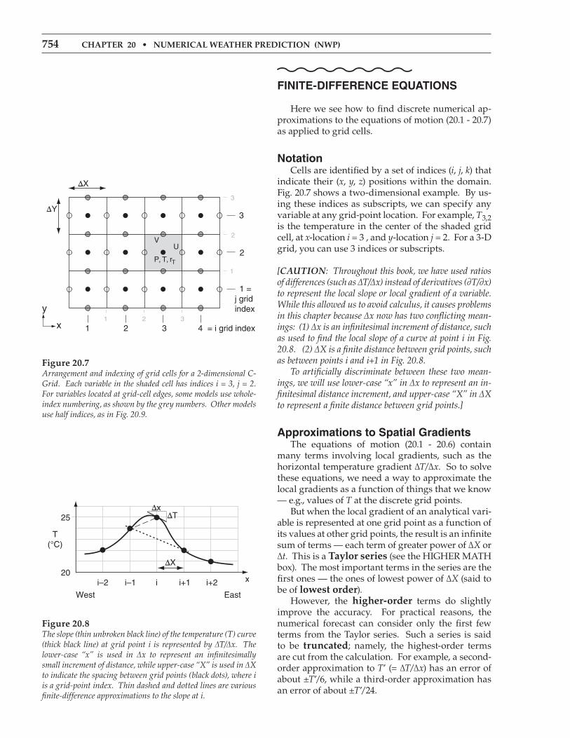
notation Cells are identified by a set of indices (i, j, k) that indicate their (x, y, z) positions within the domain. Fig. 20.7 shows a two-dimensional example. By us-ing these indices as subscripts, we can specify any variable at any grid-point location. For example, T3,2 is the temperature in the center of the shaded grid cell, at x-location i = 3 , and y-location j = 2. For a 3-D grid, you can use 3 indices or subscripts.
[CAUTION: Throughout this book, we have used ratios of differences (such as ∆T/∆x) instead of derivatives (∂T/∂x) to represent the local slope or local gradient of a variable. While this allowed us to avoid calculus, it causes problems in this chapter because ∆x now has two conflicting mean-ings: (1) ∆x is an infinitesimal increment of distance, such as used to find the local slope of a curve at point i in Fig. 20.8. (2) ∆X is a finite distance between grid points, such as between points i and i+1 in Fig. 20.8. To artificially discriminate between these two mean-ings, we will use lower-case “x” in ∆x to represent an in-finitesimal distance increment, and upper-case “X” in ∆X to represent a finite distance between grid points.]
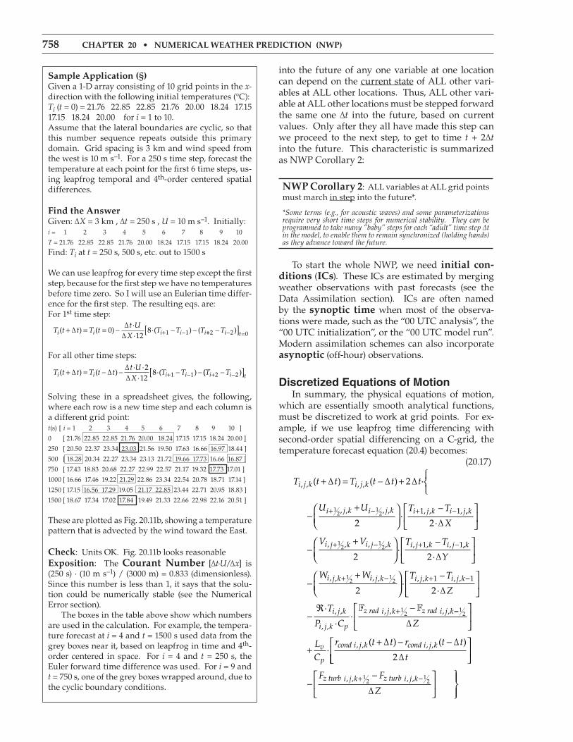
approximations to Spatial gradients The equations of motion (20.1 - 20.6) contain many terms involving local gradients, such as the horizontal temperature gradient ∆T/∆x. So to solve these equations, we need a way to approximate the local gradients as a function of things that we know — e.g., values of T at the discrete grid points. But when the local gradient of an analytical vari-able is represented at one grid point as a function of its values at other grid points, the result is an infinite sum of terms — each term of greater power of ∆X or ∆t. This is a taylor series (see the HIGHER MATH box). The most important terms in the series are the first ones — the ones of lowest power of ∆X (said to be of lowest order). However, the higher-order terms do slightly improve the accuracy. For practical reasons, the numerical forecast can consider only the first few terms from the Taylor series. Such a series is said to be truncated; namely, the highest-order terms are cut from the calculation. For example, a second-order approximation to T’ (= ∆T/∆x) has an error of about ±T’/6, while a third-order approximation has an error of about ±T’/24.
Figure 20.7Arrangement and indexing of grid cells for a 2-dimensional C-Grid. Each variable in the shaded cell has indices i = 3, j = 2. For variables located at grid-cell edges, some models use whole-index numbering, as shown by the grey numbers. Other models use half indices, as in Fig. 20.9.
Figure 20.8The slope (thin unbroken black line) of the temperature (T) curve (thick black line) at grid point i is represented by ∆T/∆x. The lower-case “x” is used in ∆x to represent an infinitesimally small increment of distance, while upper-case “X” is used in ∆X to indicate the spacing between grid points (black dots), where i is a grid-point index. Thin dashed and dotted lines are various finite-difference approximations to the slope at i.

r. Stull • Practical meteorology 755
Different approximations to the local gradients have different truncation errors. Such approxi-mations can be applied to the local gradient of any weather variable — the illustrations below focus on temperature (T) gradients. Assuming a mean wind from the west, an upwind first-order difference approximation is:
∆∆
( )∆
Tx
T TXi
i i≈− −1 (20.9)
which applies at grid point i. But first-order ap-proximations to the gradient (shown by slope of the dashed line in Fig. 20.8) can have large errors rela-tive to the actual gradient (shown by the slope of the thin black line).
A centered second-order difference gives a better approximation to the gradient at i:
∆∆
( )∆
Tx
T TXi
i i≈−+ −1 1
2 (20.10)
as sketched by the dotted line in Fig. 20.8.
An even-better centered fourth-order differ-ence for the gradient at i is: (20.11) ∆
∆ ∆( ) ( )
Tx X
T T T Ti
i i i i≈ − − −[ ]+ − + −1
128 1 1 2 2
as shown by the thin solid line in Fig. 20.8. Use similar equations for gradients of other vari-ables (U, V, W, rT, ρ). Orders higher than fourth-or-der are also used in some numerical models.
HigHer MatH • taylor Series
The equations of motion have terms such as U·∂T/∂x. We can use a Taylor series to approximate de-rivative ∂T/∂x as a function of discrete grid-point val-ues. [Notation: use T’ for ∂T/∂x, use T’’ for ∂2T/∂x2.] Any analytic function such as temperature vs. distance T(x) can be expanded into an infinite series called a taylor series if the derivatives (T’, T’’, etc.) are well behaved near x. To find the value of T at (x + ∆X), where ∆X is a small finite distance from x, use a Taylor series of the form:
(20.BA1)
T x X T xX
T xX
T x( ∆ ) ( )(∆ )
!· '( )
(∆ )!
· ''( )
(
+ ≈ + +
+
1 2
1 2
∆∆ )!
· '''( )(∆ )
!· ''''( ) ...
XT x
XT x
3 4
3 4+ +
Apply the Taylor series to grid points (Fig. 20.8), where the spatial position is indicated by an index i: (20.BA2)
T T X TX
TX
TX
i i i i i+ ≈ + + + +1
2 3
2 6∆ · '
(∆ )· ''
(∆ )· '''
(∆ ))· '''' ...
4
24Ti +
Similarly, by using –∆X in the Taylor expansion, you can estimate T upwind, at grid index i–1: (20.BA3) T T X T
XT
XT
Xi i i i i− ≈ − + − +1
2 3
2 6∆ · '
(∆ )· ''
(∆ )· '''
(∆ ))· '''' ...
4
24Ti −
For practical reasons, truncate the series to a fi-nite number of terms. The more terms you keep, the smaller the truncation error. The lowest power of the ∆X term not used defines the order of the trunca-tion. Higher-order truncations have less error.
• For a simple upwind difference (with poor, first-order error in ∆X), solve eq (20.BA3) for T’:
TT T
XO Xi
i i'( )
∆(∆ )=
−+−1 (20.BA4)
where the last term indicates the truncation error. This T’ value gives the dashed-line slope in Fig. 20.8.
• For a centered difference (with moderate, second-order error in ∆X), subtract eq. (20.BA3) from (20.BA2) and solve the result for T’:
TT T
XO Xi
i i'( )
∆(∆ )=
−++ −1 1 2
2 (20.BA5)
This T’ value gives the dotted-line slope in Fig. 20.8.
• For an even-better, 4th-order, centered difference,use: (20.BA6)
TX
T T T T O Xi i i i i'∆
( ) ( ) (∆ )= − − −[ ]++ − + −1
128 1 1 2 2
4
which is a slightly better fit to the true slope at i. In this chapter, we use ∆T/∆x in place of T’. Hence, the bullets above give approximations to ∆T/∆x.
Sample applicationFind ∆T/∆x at grid point i in Fig. 20.8 using 1, 2, & 4th order gradients, for a horizontal grid spacing of 5 km.
Find the answerGiven: Ti–2 = 22, Ti–1 = 24, Ti = 25, Ti+1 = 22, Ti+2 = 21°C from the data points in Fig. 20.8. ∆X = 5 km.Find: ∆T/∆x = ? °C km–1
For Upwind 1st-order Difference, use eq. (20.9): ∆T/∆x ≈ (25 – 24°C)/(5 km) = 0.2 °c km–1 For Centered 2nd-order Difference, use eq. (20.10): ∆T/∆x ≈ (22 – 24°C) /[2·(5 km)] = –0.2 °c km–1
For Centered 4th-order Difference, use eq. (20.11): ∆T/∆x ≈ [8·(22–24°C) – (21–22°C)]/[12·(5 km)] ≈ [ (–16 + 1)°C] /(60 km) = –0.25 °c km–1
check: Units OK. Agrees with lines in Fig. 20.8.exposition: Higher-order differences are better ap-proximations, but none give the true slope exactly.

756 chaPter 20 • Numerical Weather PredictioN (NWP)
grid computation rules For mathematical and physical consistency, the grid computation rules at left must be obeyed when making calculations with grid-point values. Rule 3 is handy because you can use it to “move” values to locations where you can then multiply by other variables while obeying Rule 1. For example, consider the temperature forecast equation (20.4) for grid point (i = 3, j = 2), for the C-grid in Fig. 20.9. The first term on the right side of eq. (20.4) is temperature advection in the x-direction. If we choose to use second-order difference eq. (20.10) at location (i,j) = (3,2), we have a mismatch because we do not have wind at that same location. Rule 1 says we can not multiply the wind times the T gradient. However, we can use Rule 3 to average the U-winds from the right and left of the temperature point, knowing that this average applies halfway be-tween the two U points. The average thus spatially coincides with the temperature gradient, so we can multiply the two factors together. For that one grid point (i,j) = (3,2), the result is: (20.12)
− ≈ −+
−
UTx
U U T T·∆∆
·,
, , , ,
3 2
3 2 2 2 4 2 212
12
222
2·∆X
where the ½ grid index numbering method was used for values at the edges of the grid cell (Fig. 20.9). The parentheses hold the average U, and the square brackets hold the centered second-order difference approximation for the local T gradient. Similarly, for any grid point (i,j), the result is: (20.13)
− ≈ −+
+ − +
UTx
U U T
i j
i j i j i j·∆∆
·,
, , ,12
12
21 −−
−T
Xi j1
2,
·∆
The spatial arrangement of all grid points used in any calculation is called a stencil. Fig. 20.9 shows the stencil for eq. (20.13). Different grid arrange-ments (Grids A - E) and different approximation or-ders will result in different stencils. Significantly, the forecast for any one grid point (such as i,j) depends on the values at other nearby grid points [such as (i–1,j) , (i–½,j) , (i+½,j) , (i+1,j) ]. In turn, forecasts at each of these points depends on values at their neighbors. This interconnectivity is summarized as NWP Corollary 1, at left. For grid points near the edges of the domain, spe-cial stencils using one-sided difference approxima-tions must be used, to avoid referencing grid points that don’t exist because they are outside of the do-main. Alternately, a halo of ghost-cell grid points outside the forecast domain can be specified using values found from a larger coarser domain or from imposed boundary conditions (Bcs; i.e., the state of the air along the edges of the forecast domain).
Figure 20.9Sketch of a two-dimensional C grid. Consider the computa-tion of temperature advection by the U wind, as contributes to the temperature tendency at the one grid point centered in the shaded cell. The grid points needed to make that calculation are outlined with the dotted line, and their arrangement is called a stencil.
Sample applicationWhat is the warming rate at grid point (i=3, j=2) in Fig. 20.9 due to temperature advection in the x-direction, given T2,2 = 22°C, T3,2 = 23°C, T4,2 = 24°C, U2½,2 = –5 m s–1, U3½,2 = –7 m s–1, ∆X = 10 km?
Find the answerGiven: T and U values above. ∆X = 10 kmFind: ∆T/∆t = –U·∆T/∆x = ? °C h–1 .
Use eq. (20.12): ∆T/∆t ≈ –0.5·(–7–5 m s–1) · [ 0.5·(24 – 22°C)/(104m) ] ≈ (6 m s–1) · [ 1°C/(104m) ] · (3600 s h–1) = 2.16 °c h–1
check: Units OK. Sign OK. Magnitude OK.exposition: Winds are advecting in warmer air from the East, causing advective warming.
NWP corollary 1: The forecast at any one point is affected by ALL other points in the forecast domain.
grid computation rules(1) When multiplying or dividing any two variables, both of those variables must be at the same point in space. The result applies at that same point.
(2) When adding, averaging, or subtracting any two vari-ables, if both those variables are at the same point in space, then the result applies at the same point.
(3) However, when adding, averaging, or subtracting two variables at different locations in space, the sum, average, or difference applies at a physical location halfway be-tween the locations of the original variables.

r. Stull • Practical meteorology 757
time Differencing The smooth flow of time implied by the left side of the equations of motion can be approximated by a sequence of discrete time steps, each of duration ∆t. For example, the temperature tendency term on the left side of eq. (20.4) can be written as a centered time difference:
∆∆
≈ + ∆ − − ∆∆
Tt
T t t T t tt
( ) ( )·2 (20.14)
When combined with the right side of eq. (20.4), the result gives the temperature at some future time as a function of the temperatures and winds at ear-lier times: (20.15)
T t t T t t t3 2 3 2 2, ,( ) ( ) ·+ ∆ = − ∆ + ∆ [ ]RHS of eq. 20.4
Typical time-step durations ∆t are on the order of a few seconds to tens of minutes, depending on the grid size (see the section on numerical stability). The equation above is a form of the leapfrog scheme. It gets its name because the forecast starts from the previous time step (t–∆t) and leaps over the present step (t) to make a forecast for the future (t+∆t). Although it leaps over the present step, it utilizes the present conditions to determine the future condi-tions. Fig. 20.10 shows a sketch of this scheme. The two leapfrog solutions (one starting at t–∆t and the other starting at t, illustrated above and be-low the time line in Fig. 20.10) sometimes diverge from each other, and need to be occasionally aver-aged together to yield a consistent forecast. Without such averaging the solution would become unstable, and would numerically blow up (see next section). There are other numerical solutions that work better than the leapfrog method. One example is the runge-Kutta method, described in the INFO Box. By combining eqs. (20.12 & 20.15), we get a tem-perature forecast equation that includes only the U-advection forcing: (20.16)
T t t T t t
tX
U U
3 2 3 2
3 2 2 212
12
, ,
, ,
( ) ( )
· ( )·
+ ∆ = − ∆ +
∆∆
+ 112 4 2 2 2T T
t, ,− where the subscript t at the very right indicates that all of the terms inside the curly brackets are evalu-ated at time t. So the future temperature (at t+∆t), depends on the current temperature and winds (at t) and on the past temperature (at t–∆t). The concept of a stencil can be extended to include the 4-D ar-rangement of locations and times needed to forecast one aspect of physics for any grid point. Generalizing the previous equation, and recall-ing NWP Corollary 1, we infer that: the forecast ∆t
Figure 20.10Time line illustrating the “leapfrog” time-differencing scheme.
info • time Differencing Methods
The prognostic equations of motion (20.1 - 20.6) can be written in a generic form:
∆A/∆t = f[A, x, t] ,
where A = any dependent variable (e.g., U, V, W, T, etc.), f is a function that describes all the dynamics and physics of the equations of motion, and x represents all other independent variables (x, y, z) as indicated by grid-point indices (i, j, k). Knowing present (at time t) and all past values at the grid points, how do we make a small time step ∆t into the future?
One of the simplest methods is called the euler method (also known as the Euler-forward method): A(t+∆t) = A(t) + ∆t · f[A(t), x, t]
But this is only first-order accurate, and is never used because errors accumulate so quickly that the numer-ical forecast often blows up (forecasts values of ± infinity) causing the computer to crash (premature termination due to computation errors).
The leapfrog method was already given in the text, and is second-order accurate. A(t+∆t) = A(t–∆t) + 2∆t · f[A(t), x, t]
Higher-order accuracy has less error.
Also popular is the fourth-order runge-Kutta method, which has even less error, but re-quires intermediate steps done in the order listed:
(1) k1 = f[ A(t) , x , t ]
(2) k2 = f[ A(t)+½∆t·k1 , x , t+½∆t ]
(3) k3 = f[ A(t)+½∆t·k2 , x , t+½∆t ]
(4) k4 = f[ A(t)+∆t·k3 , x , t+∆t ]
(5) A(t+∆t) = A(t) + (∆t/6)·[ k1 + 2k2 + 2k3 + k4 ]
758 chaPter 20 • Numerical Weather PredictioN (NWP)
into the future of any one variable at one location can depend on the current state of ALL other vari-ables at ALL other locations. Thus, ALL other vari-able at ALL other locations must be stepped forward the same one ∆t into the future, based on current values. Only after they all have made this step can we proceed to the next step, to get to time t + 2∆t into the future. This characteristic is summarized as NWP Corollary 2:
NWP corollary 2: ALL variables at ALL grid points must march in step into the future*.
*Some terms (e.g., for acoustic waves) and some parameterizations require very short time steps for numerical stability. They can be programmed to take many “baby” steps for each “adult” time step ∆t in the model, to enable them to remain synchronized (holding hands) as they advance toward the future.
To start the whole NWP, we need initial con-ditions (ics). These ICs are estimated by merging weather observations with past forecasts (see the Data Assimilation section). ICs are often named by the synoptic time when most of the observa-tions were made, such as the “00 UTC analysis”, the “00 UTC initialization”, or the “00 UTC model run”. Modern assimilation schemes can also incorporate asynoptic (off-hour) observations.
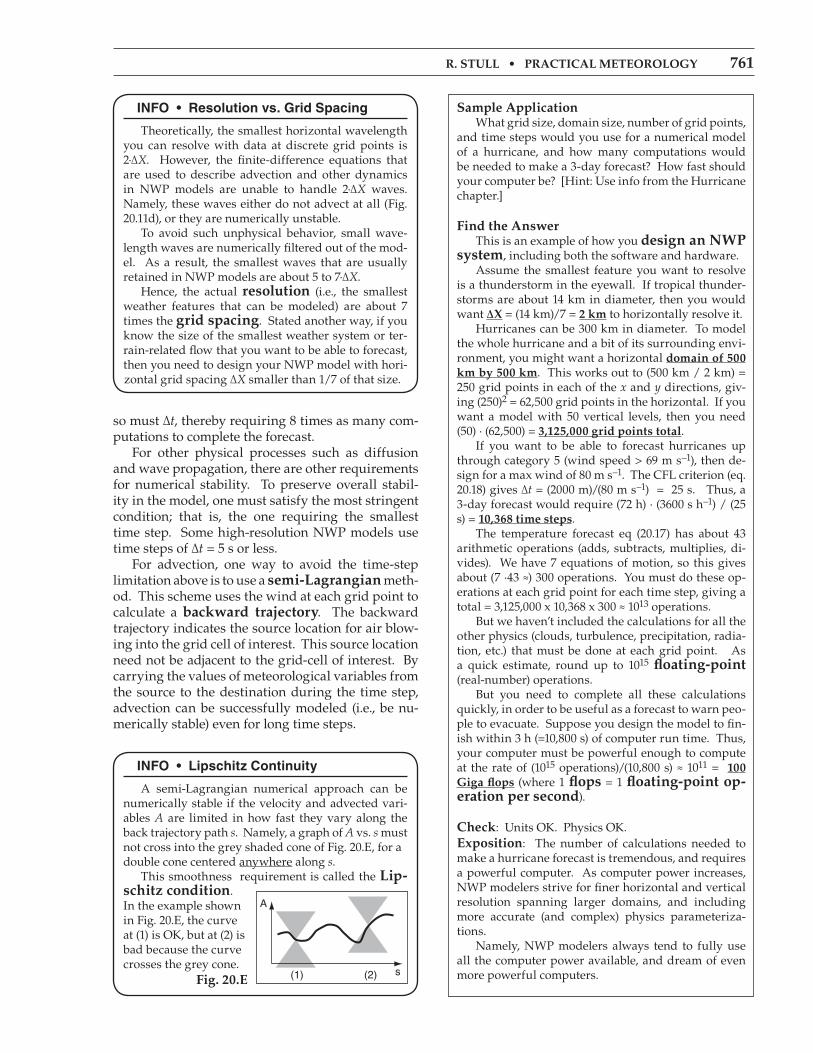
Discretized equations of Motion In summary, the physical equations of motion, which are essentially smooth analytical functions, must be discretized to work at grid points. For ex-ample, if we use leapfrog time differencing with second-order spatial differencing on a C-grid, the temperature forecast equation (20.4) becomes: (20.17)
T t t T t t ti j k i j k, , , ,( ∆ ) ( ∆ ) ∆ ·+ = − +
2
−
+
−+ − + −U U T Ti j k i j k i j k i j1
21
2
21 1, , , , , , ,
·,,
·∆k
X2
−
+
−+ − + −V V T Ti j k i j k i j k i j, , , , , , ,
·1
21
2
21 1,,
·∆k
Y2
−
+
−+ − +W W T Ti j k i j k i j k i j k, , , , , , , ,
·1
21
2
21 −−
1
2·∆Z
−
ℜ −+·
··
, ,
, ,
, , , ,T
P Ci j k
i j k p
z rad i j k z rad i j kF F12 −−
12
∆Z
+
+ − −LC
r t t r t t
tv
p
cond i j k cond i j k·
( ∆ ) ( ∆ )
∆, , , ,
2
−
−
+ −F F
Zz turb i j k z turb i j k, , , ,
∆
12
12
Sample application (§)Given a 1-D array consisting of 10 grid points in the x-direction with the following initial temperatures (°C):Ti (t = 0) = 21.76 22.85 22.85 21.76 20.00 18.24 17.15 17.15 18.24 20.00 for i = 1 to 10. Assume that the lateral boundaries are cyclic, so that this number sequence repeats outside this primary domain. Grid spacing is 3 km and wind speed from the west is 10 m s–1. For a 250 s time step, forecast the temperature at each point for the first 6 time steps, us-ing leapfrog temporal and 4th-order centered spatial differences.
Find the answerGiven: ∆X = 3 km , ∆t = 250 s , U = 10 m s–1. Initially:i = 1 2 3 4 5 6 7 8 9 10
T = 21.76 22.85 22.85 21.76 20.00 18.24 17.15 17.15 18.24 20.00
Find: Ti at t = 250 s, 500 s, etc. out to 1500 s
We can use leapfrog for every time step except the first step, because for the first step we have no temperatures before time zero. So I will use an Eulerian time differ-ence for the first step. The resulting eqs. are:For 1st time step:
T t t T tt U
XT T Ti i i i i( ∆ ) ( )
∆ ·∆ ·
·( ) (+ = = − − −+ −012
8 1 1 ++ − =−[ ]2 2 0Ti t)
For all other time steps:
T t t T t tt UX
T Ti i i i( ∆ ) ( ∆ )∆ · ·∆ ·
·( )+ = − − − −+ −2
128 1 1 (( )T Ti i t+ −−[ ]2 2
Solving these in a spreadsheet gives, the following, where each row is a new time step and each column is a different grid point:t(s) [ i = 1 2 3 4 5 6 7 8 9 10 ]
0 [ 21.76 22.85 22.85 21.76 20.00 18.24 17.15 17.15 18.24 20.00 ]
250 [ 20.50 22.37 23.34 23.03 21.56 19.50 17.63 16.66 16.97 18.44 ]
500 [ 18.28 20.34 22.27 23.34 23.13 21.72 19.66 17.73 16.66 16.87 ]
750 [ 17.43 18.83 20.68 22.27 22.99 22.57 21.17 19.32 17.73 17.01 ]
1000 [ 16.66 17.46 19.22 21.29 22.86 23.34 22.54 20.78 18.71 17.14 ]
1250 [ 17.15 16.56 17.29 19.05 21.17 22.85 23.44 22.71 20.95 18.83 ]
1500 [ 18.67 17.34 17.02 17.84 19.49 21.33 22.66 22.98 22.16 20.51 ]
These are plotted as Fig. 20.11b, showing a temperature pattern that is advected by the wind toward the East.
check: Units OK. Fig. 20.11b looks reasonableexposition: The courant Number [∆t·U/∆x] is (250 s) · (10 m s–1) / (3000 m) = 0.833 (dimensionless). Since this number is less than 1, it says that the solu-tion could be numerically stable (see the Numerical Error section). The boxes in the table above show which numbers are used in the calculation. For example, the tempera-ture forecast at i = 4 and t = 1500 s used data from the grey boxes near it, based on leapfrog in time and 4th-order centered in space. For i = 4 and t = 250 s, the Euler forward time difference was used. For i = 9 and t = 750 s, one of the grey boxes wrapped around, due to the cyclic boundary conditions.

r. Stull • Practical meteorology 759
Finite-difference equations that are used to fore-cast winds and humidity are similar. If we had used higher-order differencing, and included the curva-ture terms and mapping factors, the result would have contained even more terms. Although the equation above looks complicated, it is trivial for a digital computer to solve because it is just algebra. Computing this equation takes a finite time — perhaps a few microseconds. Similar computation time must be spent for all the other grid points in the domain. These computations must be repeated for a succession of short time steps to reach forecast durations of several days. Thus, for many grid points and many time steps, the total computer run-time accumulates and can take many minutes to several hours on powerful computers.
nuMericaL errorS & inStaBiLity
Causes of NWP errors include round-off error, truncation error, numerical instability, and dy-namical instability. Dynamical instability related to initial-condition errors will be discussed later in the section on chaos. Additional errors not consid-ered in this section are coding bugs, computer vi-ruses, user errors, numerical or physical approxima-tions, simplifications and parameterizations.
round-off error round-off error exists because computers rep-resent numbers by a limited number of binary bits (e.g., 32, 64, 128 bits). As a result, some real decimal numbers can be only approximately represented inthe computer. For example, a 32-bit computer can resolve real numbers that are different from each other by about 3x10⁻⁸ or greater. Any finer differ-ences are missed. To demonstrate, I wrote a computer program to start with x = 0.0, and then repeatedly add 0.1 to x (printing x at each step) until it reaches x = 3.0, at which point I programmed it to stop. When I used single precision (32-bits), my program never stopped. After 30 additions it had found x = 2.9999993, but since this was not exactly equal to 3.0, the program kept adding 0.1 in an infinite loop (i.e., ran forever). When I tried it again using double precision (64 bits) it also never stopped, getting only as close to 3.0 as x = 3.0000000000000013 . Namely, the slight error between decimal and bi-nary representations of a number can accumulate, or can cause unexpected outcomes of conditional tests (“if” statements). Most modern computers use many bits to represent numbers. Nonetheless, always con-sider round-off errors when you write programs.
info • early History of nWP
The first equations of fluid mechanics were formu-lated by Leonhard Euler in 1755, using the differential calculus invented by Isaac Newton in 1665, Gottfried Wilhelm Leibniz in 1675, and using partial deriva-tives devised by Jean le Rond d’Alembert in 1746. Terms for molecular viscosity were added by Claude-Louis Navier in 1827 and George Stokes in 1845. The equations describing fluid motion are of-ten called the Navier-Stokes equations. These primitive equations for fluid mechanics were refined by Herman von Helmholtz in 1888. About a decade later Vilhelm Bjerknes in Norway suggested that these same equations could be used for the atmosphere. He was a very strong proponent of using physics, rather than empirical rules, for mak-ing weather forecasts. In 1922, Lewis Fry Richardson in England pub-lished a book describing the first experimental nu-merical weather forecast — which he made by solv-ing the primitive equations with mechanical desk calculators. His book was very highly regarded and well received as one of the first works that combined physics and dynamics in a thorough, interactive way. It took him 6 weeks to make a 6 h forecast. Unfor-tunately, his forecast of surface pressure was off by an order of magnitude compared to the real weather. Because of the great care that Richardson took in pro-ducing these forecasts, most of his peers concluded that NWP was not feasible. This discouraged further work on NWP until two decades later. John von Neumann, a physicist at Princeton Uni-versity’s Institute for Advanced Studies, and Vladimir Zworykin, an electronics scientist at RCA’s Princeton Laboratories and key inventor of television, proposed in 1945 to initiate NWP as a way to demonstrate the potential of the recently-invented electronic comput-ers. Their goal was to simulate the global circulation. During the first few years they could not agree on how to approach the problem. Von Neumann formed a team of theoretical mete-orologists including Carl-Gustav Rossby, Arnt Elias-sen, Jule Charney, and George Platzman. They real-ized the need to simplify the full primitive equations in order to focus their limited computer power on the long waves of the global circulation. So Charney and von Neumann developed a simple one-layer baro-tropic model (conservation of absolute vorticity). Their first electronic computer, the ENIAC, filled a large room at Princeton, and used vacuum tubes that generated tremendous heat and frequently burned out. The research team had to translate the differ-ential equations into discrete form, write the code in machine language (FORTRAN and C had not yet been invented), decide how large a forecast domain was necessary, and do many preliminary calculations using slide rules and mechanical calculators. Their first ENIAC forecasts were made in March-April 1950, for three weather case studies over North America. This was the start of modern NWP.

760 chaPter 20 • Numerical Weather PredictioN (NWP)
truncation error truncation error was already discussed, and refers to the neglect (i.e., truncation) of higher-order terms in a Taylor series approximation to local gra-dients. If we retain more terms in the Taylor series, then the result is a higher-order solution that is more accurate, but which takes longer to run because there are more terms to compute. If we truncate the series at lower order, the numerical solution is faster but less accurate. In NWP, time and space difference schemes are chosen as a compromise between accu-racy and speed.
numerical instability Numerical instability causes forecasts to blow up. Namely, the numerical solution rapidly diverges from the true solution, can have incorrect sign, and can approach unphysical values (±∞). Truncation er-ror is one cause of numerical instability. Numerical instability can also occur if the wind speeds are large, the grid size is small, and the time step is too large. For example, eq. (20.16) models advection by using temperature in neighboring grid cells. But what happens if the wind speed is so strong that temperature from a more distant location in the real atmosphere (beyond the neighboring cell) can arrive during the time step ∆t? Such a physical situation is not accounted for in the numerical ap-proximation of eq. (20.16). This can create numerical errors that amplify, causing the model to blow up (see Fig. 20.11). Such errors can be minimized by taking a small enough time step. The specific requirement for sta-bility of advection processes in one dimension is
∆ ≤ ∆t
XU
•(20.18)
with similar requirements in the y and z direc-tions. This is known as the courant-Friedrichs-lewy (cFl) stability criterion, or the courant condition. When modelers use finer mesh grids with smaller ∆X values, they must also reduce ∆t to preserve numerical stability. The combined effect greatly increases model run time on the computer. For example, if ∆X and ∆Y are reduced by half, then
Figure 20.11 (at left)Examples of numerical stability for advection, with ∆X = 3 km and U = 10 m s–1. Thick black line is initial condition, and the forecast after each time step is shown as lighter grey, with the last (6th) step dotted. A temperature signal of wavelength 10·∆X is numerically stable for time steps ∆t of (a) 100 s and (b) 250 s, but (c) = 450 s exceeds the CFL criterion, and the solution blows up (i.e., the wave amplitude increases without bound). (d) A 2·∆X wave does not advect at all (i.e., is unphysical).
r. Stull • Practical meteorology 761
so must ∆t, thereby requiring 8 times as many com-putations to complete the forecast. For other physical processes such as diffusion and wave propagation, there are other requirements for numerical stability. To preserve overall stabil-ity in the model, one must satisfy the most stringent condition; that is, the one requiring the smallest time step. Some high-resolution NWP models use time steps of ∆t = 5 s or less. For advection, one way to avoid the time-step limitation above is to use a semi-lagrangian meth-od. This scheme uses the wind at each grid point to calculate a backward trajectory. The backward trajectory indicates the source location for air blow-ing into the grid cell of interest. This source location need not be adjacent to the grid-cell of interest. By carrying the values of meteorological variables from the source to the destination during the time step, advection can be successfully modeled (i.e., be nu-merically stable) even for long time steps.
info • resolution vs. grid Spacing
Theoretically, the smallest horizontal wavelength you can resolve with data at discrete grid points is 2·∆X. However, the finite-difference equations that are used to describe advection and other dynamics in NWP models are unable to handle 2·∆X waves. Namely, these waves either do not advect at all (Fig. 20.11d), or they are numerically unstable. To avoid such unphysical behavior, small wave-length waves are numerically filtered out of the mod-el. As a result, the smallest waves that are usually retained in NWP models are about 5 to 7·∆X. Hence, the actual resolution (i.e., the smallest weather features that can be modeled) are about 7 times the grid spacing. Stated another way, if you know the size of the smallest weather system or ter-rain-related flow that you want to be able to forecast, then you need to design your NWP model with hori-zontal grid spacing ∆X smaller than 1/7 of that size.
Sample application What grid size, domain size, number of grid points, and time steps would you use for a numerical model of a hurricane, and how many computations would be needed to make a 3-day forecast? How fast should your computer be? [Hint: Use info from the Hurricane chapter.]
Find the answer This is an example of how you design an NWP system, including both the software and hardware. Assume the smallest feature you want to resolve is a thunderstorm in the eyewall. If tropical thunder-storms are about 14 km in diameter, then you would want ∆X = (14 km)/7 = 2 km to horizontally resolve it. Hurricanes can be 300 km in diameter. To model the whole hurricane and a bit of its surrounding envi-ronment, you might want a horizontal domain of 500 km by 500 km. This works out to (500 km / 2 km) = 250 grid points in each of the x and y directions, giv-ing (250)2 = 62,500 grid points in the horizontal. If you want a model with 50 vertical levels, then you need (50) · (62,500) = 3,125,000 grid points total. If you want to be able to forecast hurricanes up through category 5 (wind speed > 69 m s–1), then de-sign for a max wind of 80 m s–1. The CFL criterion (eq. 20.18) gives ∆t = (2000 m)/(80 m s–1) = 25 s. Thus, a 3-day forecast would require (72 h) · (3600 s h–1) / (25 s) = 10,368 time steps. The temperature forecast eq (20.17) has about 43 arithmetic operations (adds, subtracts, multiplies, di-vides). We have 7 equations of motion, so this gives about (7 ·43 ≈) 300 operations. You must do these op-erations at each grid point for each time step, giving a total = 3,125,000 x 10,368 x 300 ≈ 1013 operations. But we haven’t included the calculations for all the other physics (clouds, turbulence, precipitation, radia-tion, etc.) that must be done at each grid point. As a quick estimate, round up to 1015 floating-point (real-number) operations. But you need to complete all these calculations quickly, in order to be useful as a forecast to warn peo-ple to evacuate. Suppose you design the model to fin-ish within 3 h (=10,800 s) of computer run time. Thus, your computer must be powerful enough to compute at the rate of (1015 operations)/(10,800 s) ≈ 1011 = 100 giga flops (where 1 flops = 1 floating-point op-eration per second).
check: Units OK. Physics OK.exposition: The number of calculations needed to make a hurricane forecast is tremendous, and requires a powerful computer. As computer power increases, NWP modelers strive for finer horizontal and vertical resolution spanning larger domains, and including more accurate (and complex) physics parameteriza-tions. Namely, NWP modelers always tend to fully use all the computer power available, and dream of even more powerful computers.
info • Lipschitz continuity
A semi-Lagrangian numerical approach can be numerically stable if the velocity and advected vari-ables A are limited in how fast they vary along the back trajectory path s. Namely, a graph of A vs. s must not cross into the grey shaded cone of Fig. 20.E, for adouble cone centered anywhere along s. This smoothness requirement is called the lip-schitz condition. In the example shown in Fig. 20.E, the curve at (1) is OK, but at (2) is bad because the curve crosses the grey cone. Fig. 20.e
762 chaPter 20 • Numerical Weather PredictioN (NWP)
tHe nuMericaL forecaSt ProceSS
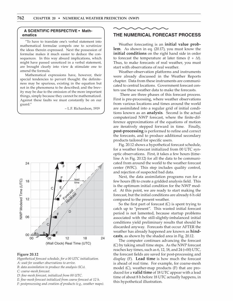
Weather forecasting is an initial value prob-lem. As shown in eq. (20.17), you must know the initial conditions on the right hand side in order to forecast the temperature at later times (t + ∆t). Thus, to make forecasts of real weather, you must start with observations of real weather. Weather-observation platforms and instruments were already discussed in the Weather Reports chapter. Data from these instruments are communi-cated to central locations. Government forecast cen-ters use these weather data to make the forecasts. There are three phases of this forecast process. First is pre-processing, where weather observations from various locations and times around the world are assimilated into a regular grid of initial condi-tions known as an analysis. Second is the actual computerized NWP forecast, where the finite-dif-ference approximations of the equations of motion are iteratively stepped forward in time. Finally, post-processing is performed to refine and correct the forecasts, and to produce additional secondary products tailored for specific users. Fig. 20.12 shows a hypothetical forecast schedule, for a weather forecast initialized from 00 UTC syn-optic observations. First, it takes a few hours (time-line A in Fig. 20.12) for all the data to be communi-cated from around the world to the weather forecast center (WFC). This step includes quality control, and rejection of suspected bad data. Next, the data assimilation programs run for a few hours (B) to create a gridded analysis field. This is the optimum initial condition for the NWP mod-el. At this point, we are ready to start making the forecast, but the initial conditions are already 6 h old compared to the present weather. So the first part of forecast (C) is spent trying to catch up to “present”. This wasted initial forecast period is not lamented, because startup problems associated with the still-slightly-imbalanced initial conditions yield preliminary results that should be discarded anyway. Forecasts that occur AFTER the weather has already happened are known as hind-casts, as shown by the shaded area in Fig. 20.12. The computer continues advancing the forecast (C) by taking small time steps. As the NWP forecast reaches key times, such as 6, 12, 18, and 24 (=00) UTC, the forecast fields are saved for post-processing and display (F). lead time is how much the forecast is ahead of real time. For example, for coarse-mesh model (C), weather-map products (F) that are pro-duced for a valid time of 18 UTC appear with a lead time of about 8 h before 18 UTC actually happens, in this hypothetical illustration.
Figure 20.12Hypothetical forecast schedule, for a 00 UTC initialization. A: wait for weather observations to arrive. B: data assimilation to produce the analysis (ICs).C: coarse-mesh forecast. D: fine-mesh forecast, initialized from 00 UTC. E: fine-mesh forecast initialized from coarse forecast at 12 h.F: postprocessing and creation of products (e.g., weather maps).
a Scientific PerSPectiVe • Math-ematics
“To have to translate one’s verbal statement into mathematical formulae compels one to scrutinize the ideas therein expressed. Next the possession of formulae makes it much easier to deduce the con-sequences. In this way absurd implications, which might have passed unnoticed in a verbal statement, are brought clearly into view & stimulate one to amend the formula. Mathematical expressions have, however, their special tendencies to pervert thought: the definite-ness may be spurious, existing in the equation but not in the phenomena to be described; and the brev-ity may be due to the omission of the more important things, simply because they cannot be mathematized. Against these faults we must constantly be on our guard.” – L.F. Richardson, 1919
r. Stull • Practical meteorology 763
Fig. 20.12 shows a coarse-mesh model (C) that takes 3 h of computation for each 24 h of forecast, as indicated by the slope of line (C). A finer-mesh model might take longer to run (with gentler slope). Model (D) takes 18 h to make a 24 h forecast, and if initialized from the 00 UTC initial conditions, might never catch up to the real weather during Day 1. Hence, it would be useless as a forecast — it would never escape from the hindcast domain. But for one-way nesting, a fine-mesh forecast (E) could be initialized from the 12 UTC coarse-mesh forecast. This is analogous to a multi-stage rocket, where the coarse mesh (C) blasts the forecast from the past to the future, and then the finer-mesh (E) can remain in the future even though E has the same slope as D. NWP meteorologists always have the need for speed. Faster computers allow most phases of the forecast process to run faster, allowing finer-resolu-tion forecasts over larger domains with more accu-racy and greater lead time. Speed-up can also be achieved computationally by making the dynamics and physics subroutines run faster, by utilizing more processor cores, and by utilizing special computer chips such as graphics Processing units (gPus). However, tremendous speed-up of a few subroutines might cause only a small speed-up in the overall run time of the NWP model, as explained by amdahl’s law (see INFO Box). The actual duration of phases (A) through (F) vary with the numerical forecast center, depending on their data-assimilation method, model numerics, domain size, grid resolution, and computer power. Details of the forecast phases are explained next.
Balanced Mass and flow fields Over the past few decades it was learned by hard experience that numerical models give bad forecasts if they are initialized with the raw observed data. One reason is that the in-situ observation network has large gaps, such as over the oceans and in much of the Southern Hemisphere. Also, while there are many observations at the surface, there are fewer in-situ observations aloft. Remote sensors on satellites do not observe many of the needed dynamic vari-ables (U, V, W, T, rT, ρ) directly, and have very poor vertical resolution. Observations can also contain errors, and local flow around mountains or trees can cause observations that are not representative of the larger-scale flow. The net effect of such gaps, errors, and inconsis-tencies is that the numerical representation of this initial condition is imbalanced. By imbalanced, we mean that the observed winds disagree with the theoretical winds, where theoretical winds such as
info • amdahl’s Law
Computer architect Gene Amdahl described the overall speedup factor SALL of a computer program as a function of the speedup Si of individual subrou-tines, where Pi is the portion of the total computation done by subroutine i:
S P SALL i i= ∑ −( / )
1
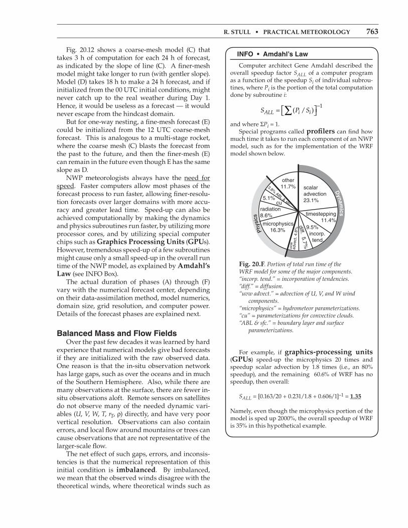
and where ΣPi = 1. Special programs called profilers can find how much time it takes to run each component of an NWP model, such as for the implementation of the WRF model shown below.
Fig. 20.F. Portion of total run time of the WRF model for some of the major components. “incorp. tend.” = incorporation of tendencies. “diff.” = diffusion. “uvw advect.” = advection of U, V, and W wind components. “microphysics” = hydrometeor parameterizations. “cu” = parameterizations for convective clouds. “ABL & sfc.” = boundary layer and surface parameterizations.
For example, if graphics-processing units (gPus) speed-up the microphysics 20 times and speedup scalar advection by 1.8 times (i.e., an 80% speedup), and the remaining 60.6% of WRF has no speedup, then overall:
SALL = [0.163/20 + 0.231/1.8 + 0.606/1]–1 = 1.35
Namely, even though the microphysics portion of the model is sped up 2000%, the overall speedup of WRF is 35% in this hypothetical example.

764 chaPter 20 • Numerical Weather PredictioN (NWP)
the geostrophic wind are based on temperature and pressure fields via atmospheric dynamics. Balanced and imbalanced flows can be illustrat-ed with a pond of water. Suppose initially the wa-ter-level is everywhere level, and the water currents and waves are zero (Fig. 20.13a). This flow system is balanced, because with a level pond surface we indeed expect no currents or waves. Next, add extra water to the center of the pond (Fig. 20.13b). This mass field (i.e., the distribution of water mass in the pond) is not balanced with the flow field (i.e., the motions or circulations within the pond, which for Fig. 20.13b are assumed to be zero). This imbal-ance causes waves and currents to form (Fig. 20.13c), which help to redistribute mass. These transient waves and currents decay, leaving the pond in a new balanced state (i.e., level water surface, no waves, no currents), but with slightly greater water depth. Consider what happens to a numerical model of the pond if observation errors are incorporated into the initial conditions. Suppose that the water level in the center of the numerical pond is erroneously “observed” to be 1 m higher than the level every-where else (Fig. 20.13b). Namely, the “true” initial conditions might be like Fig. 20.13a, but observation errors might cause the “modeled” initial conditions to be like Fig. 20.13b. A well-designed numerical model of a pond would simulate the dynamical behavior of an actual pond. Hence, the modeled pond would respond as in Figs. 20.13c & d, even though the actual pond would remain motionless as in Fig. 20.13a. The transient waves and currents are an artifact of the poor initial conditions in the model, and are not representative of the true flow in the real pond. Hence, the forecast results are not to be trusted dur-ing the first few minutes of the forecast period while the model is adjusting itself to a balanced state. Numerical forecasts of the atmosphere have the same problem, but on a longer time scale than a pond. Namely, the first 0.5 to 3 hours of a weather forecast are relatively useless while the model adjusts to imbalances in the initial conditions (see the Data Assimilation section). During this startup period, simulated atmospheric waves are bouncing around in the model, both vertically and horizontally. After the first 3 to 12 h of forecast, the dynam-ics are fairly well balanced, and give essentially the same forecast as if the fields were balanced from the start. However, spurious waves in the model might also cause unjustified rejection of good data during data assimilation (see next subsection). Also, the erroneous waves can generate errone-ous clouds that cause erroneous precipitation, etc. The net result could be an unrealistic loss of water from the model that could reduce the chance of fu-ture cloud formation and precipitation. Change of
Figure 20.13Demonstration of a dynamic system becoming balanced. (a) Balanced initial state of a pond of water (shaded grey), with no waves and no currents. (b) Extra water added in center of pond, causing the water-mass distribution to not be in equilibrium with the waves and currents. (c) Wave generation as the pond adjusts itself toward a new balanced state. (d) Final balanced state with slightly higher water everywhere, but no waves and no currents.

r. Stull • Practical meteorology 765
water content is just one of many irreversible pro-cesses that can permanently harm the forecast. In summary, initialization problems cause a transient period of poor forecast quality, and can permanently degrade longer-term forecast skill or cause rejection of good data. Hence, data-assimila-tion methods to reduce startup imbalances, such as described next, are highly desirable.
Data assimilation and analysis The technique of incorporating observations into the model’s initial conditions is called data assimi-lation. Most assimilation techniques capitalize on the tendency of NWP models to create a balanced state during their forecasts. One can utilize the balanced state from a previ-ous forecast as a first guess of the initial conditions for a new forecast. When new weather observations are incorporated with the first guess, the result is called a weather analysis. To illustrate the initialization process, suppose a forecast was started using initial conditions at 00 UTC, and that a 6-hour forecast was produced, valid at 06 UTC. This 06 UTC forecast could serve as the first guess for new initial conditions, into which the new 06 UTC weather observations could be incor-porated. The resulting 06 UTC analysis could then be used as the initial conditions to start the next forecast run. The process could then be repeated for successive forecasts started every 6 h. Although the analysis represents current or re-cent-past weather (not a forecast), the analyzed field is usually not exactly equal to the raw observations because the analysis has been smoothed and par-tially balanced. Observations are used as follows. First, an automated initial screening of the raw data is performed. During this quality control phase, some observations are rejected because they are unphysical (e.g., negative humidities), or they disagree with most of the surrounding observations. In locations of the world where the observation net-work is especially dense, neighboring observations are averaged together to make a smaller number of statistically-robust observations. When incorporating the remaining weather ob-servations into the analysis, the raw data from vari-ous sources are not treated equally. Some sources have greater likelihood of errors, and are weighted less than those observations of higher quality. Also, observations made slightly too early or too late, or made at a different altitude, are weighted less. In some locations such as the tropics where Coriolis force and pressure-gradients are weak, more weight can be given to the winds than to the pressures. We focus on two data-assimilation methods here: optimum interpolation and variational. Both are
info • the Pacific Data Void
One hazard of data assimilation is that the result-ing analysis does not represent truth, because the analysis includes a previous forecast as a first guess. If the previous forecast was wrong, then the subse-quent analysis is poor. Even worse are situations where there are little or no observation data. For data-sparse regions, the first-guess from the previous forecast dominates the “analysis”. This means that future forecasts start from old forecasts, not from observations. Forecast errors tend to accumulate and amplify, causing very poor forecast skill further downstream. One such region is over the N.E. Pacific Ocean. From Fig. 9.23 in the Weather Reports & Map Analysis chapter, there are no rawinsonde observations (RAO-Bs) in that region to provide data at the dynamically important mid-tropospheric altitudes. Ships and buoys provide some surface data, and aircraft and satellites provide data near the tropopause, but there is a sparsity of data in the middle. This is known as the Pacific data void. Poor forecast skill is indeed observed downstream of this data void, in British Columbia, Canada, and Washington and Oregon, USA. The weather-forecast difficulty there is exacerbated by the complex terrain of mountains and shoreline.
info • giving a Weather Briefing
NWP forecast maps make up an important part of most weather briefings, but they should not be the only part. Bosart (2003), Snelling (1982), West (2011), and others recommend the following:
Your discussion should answer 6 questions: • What has happened? • Why has it happened?
• What is happening? • Why is it happening?
• What will happen? • Why will it happen?
Identify forecast issues throughout your briefing: • Difficult/tricky forecast details. • Significant/interesting weather.
Go from the large-scale to the smaller scales. Verify your previous forecast. Encourage questions, discussion, and debate.
For the past and current weather portions of the briefing, show satellite images/animations, radar im-ages/animations, soundings, and weather analyses. Speak clearly, concisely, loudly, and with confi-dence. No forecast is perfect, but do the best you can.
Your audience will appreciate your sincerity.

766 chaPter 20 • Numerical Weather PredictioN (NWP)
objective analysis methods in the sense that they are calculated by computer based on equations, in contrast to a “subjective analysis” by a human (such as was demonstrated in the Map Analysis chapter).
objective optimum interpolation Let σo be the standard deviation of raw-observa-tion errors from a sensor such as a rawinsonde (Ta-ble 20-2). Larger σ indicates larger errors. Let σf be the standard deviation of errors associ-ated with the first guess from a previous forecast. These are also known as background errors. Gen-erally, error increases with increasing forecast range. For example, some global NWP models have the fol-lowing errors for geopotential height Z of the 50-kPa isobaric surface:
σZf a t= · (20.19)
where a ≈ 11 m day–1 and t is forecast time range. Namely, a first guess from a 2-day forecast is less accurate (has greater error) than a first guess from a 1-day forecast. An optimum interpolation analysis weights the first guess F and the observation O according to their errors to produce an analysis field A:
A F Oo
f o
f
f o=
++
+· ·
σσ σ
σ
σ σ
2
2 2
2
2 2 (20.20)
where A, F, O , and σ all apply to the same one weather element, such as pressure, temperature, or wind. If the observation has larger errors than the first guess, then the analysis weights the observa-tion less and the first-guess more. The equation above can be used to define a cost function J:
J AF A O A
f o( )
( ) ( )= − + −
12
2
2
2
2σ σ (20.21)
where the optimum analysis from eq. (20.20) gives the minimum cost for eq. (20.21). Optimum interpolation is “local” in the sense that it considers only the observations near a grid point when producing an analysis for that point. Optimum interpolation is not perfect, leaving some imbalances that cause atmospheric gravity waves to form in the subsequent forecast. A normal-mode initialization modifies the analysis further by re-moving the characteristics that might excite gravity waves.
table 20-2. Standard deviation σo of observation errors.
Sensor type σo
Wind errors in the lower troposphere: Surface stations and ship obs Drifting buoy Rawinsonde, wind profiler Aircraft and satellite
(m s–1)3 to 45 to 6
0.5 to 2.73
Pressure errors: Surface weather stations & Rawinsonde Ship and drifting buoy S. Hemisphere manual analysis
(kPa)0.10.20.4
geopotential height errors: Surface weather stations Ship and drifting buoy S. Hemisphere manual analysis Rawinsonde
(m)71432
13 to 26
temperature errors: ASOS surface automatic weather stn. Rawinsonde upper-air obs at z < 15 km at altitudes near 30 km
(°C)0.5 to 1.0
0.5< 1.5
humidity errors: ASOS surface weather stations: Td (°C) Rawinsonde in lower troposph. RH (%) near tropopause: RH (%)
0.6 to 4.4515
Sample application A drifting buoy observes a wind of M = 10 m s–1, while the first guess for the same location gives an 8 m s–1 wind with 2 m s–1 likely error. Find the analysis wind speed.
Find the answerGiven: MO = 10 m s–1, MF = 8 m s–1, σf = 2 m s–1
Find: MA = ? m s–1
Use Table 20-2 for Wind Errors: Drifting buoy: σo = 6 m s–1
Use eq. (20.20) for wind speed M:
M M MA F
o
f oO
f
f o=
++
+· ·
σσ σ
σ
σ σ
2
2 2
2
2 2
MA =+
+( )·( )
( ) ( )( )·
(8
6
2 610
22
2 2m/sm/s
m/s m/sm/s
mm/s
m/s m/s
)
( ) ( )
2
2 22 6+
= (8 m s–1)·(36/40) + (10 m s–1)·(4/40) = 8.2 m s–1
check: Units OK. Physics OK.exposition: Because the drifting buoy has such a large error, it is given very little weight in producing the analysis. If it had been given equal weight as the first guess, then the average of the two would have been 9 m s–1. It might seem disconcerting to devalue a real observation compared to the artificial value of the first guess, but it is needed to avoid startup problems.
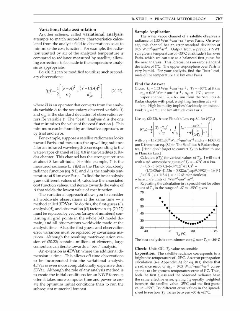
r. Stull • Practical meteorology 767
Variational data assimilation Another scheme, called variational analysis, attempts to match secondary characteristics calcu-lated from the analysis field to observations so as to minimize the cost function. For example, the radia-tion emitted by air of the analyzed temperature is compared to radiance measured by satellite, allow-ing corrections to be made to the temperature analy-sis as appropriate. Eq. (20.21) can be modified to utilize such second-ary observations:
J AF A Y H A
f yo( )
( )=
−( ) +−( )
12
2
2
2
2σ σ (20.22)
where H is an operator that converts from the analy-sis variable A to the secondary observed variable Y, and σyo is the standard deviation of observation er-rors for variable Y. The “best” analysis A is the one that minimizes the value of the cost function J. This minimum can be found by an iterative approach, or by trial and error. For example, suppose a satellite radiometer looks toward Paris, and measures the upwelling radiance L for an infrared wavelength λ corresponding to the water-vapor channel of Fig. 8.8 in the Satellites & Ra-dar chapter. This channel has the strongest returns at about 8 km altitude. For this example, Y is the measured radiance L. H(A) is the Planck blackbody radiance function (eq. 8.1), and A is the analysis tem-perature at 8 km over Paris. To find the best analysis: guess different values of A, calculate the associated cost function values, and iterate towards the value of A that yields the lowest value of cost function. The variational approach allows you to consider all worldwide observations at the same time — a method called 3dVar. To do this, the first-guess (F), analysis (A), and observation (O) factors in eq. (20.22) must be replaced by vectors (arrays of numbers) con-taining all grid points in the whole 3-D model do-main, and all observations worldwide made at the analysis time. Also, the first-guess and observation error variances must be replaced by covariance ma-trices. Although the resulting matrix-equation ver-sion of (20.22) contains millions of elements, large computers can iterate towards a “best” analysis. An extension is 4dVar, where the additional di-mension is time. This allows off-time observations to be incorporated into the variational analysis. 4DVar is even more computationally expensive than 3DVar. Although the role of any analysis method is to create the initial conditions for an NWP forecast, often it takes more computer time and power to cre-ate the optimum initial conditions than to run the subsequent numerical forecast.
Sample application The water vapor channel of a satellite observes a radiance of 1.53 W·m–2·µm–1·sr–1 over Paris. On aver-age, this channel has an error standard deviation of 0.05 W·m–2·µm–1·sr–1. Output from a previous NWP run gives a temperature of –35°C at altitude 8 km over Paris, which we can use as a balanced first guess for the new analysis. This forecast has an error standard deviation of 1°C. The upper troposphere over Paris is very humid. For your analysis, find the “best” esti-mate of the temperature at 8 km over Paris.
Find the answerGiven: Lo = 1.53 W·m–2·µm–1·sr–1 , TF = –35°C at 8 km σLo = 0.05 W·m–2·µm–1·sr–1 , σTf = 1°C , water- vapor channel: λ = 6.7 µm from the Satellites & Radar chapter with peak weighting function at z ≈ 8 km. High humidity implies blackbody emissions.Find: TA = ? °C at 8 km altitude over Paris.
Use eq. (20.22), & use Planck’s Law eq. 8.1 for H(TA)
J T T T L
c
cAF A
Tf Lo
oB
( ) ( )·
exp·
= − +−
−12
12
2 2
15
2σ σ
λ
λ TTA
−
1
2
with c1B = 1.191043x10⁸ W·m–2·µm4·sr–1 and c2 = 14387.75 µm K from near eq. (8.1) in The Satellites & Radar chap-ter. [Hint: don’t forget to convert TA in Kelvin to use in Planck’s Law.] Calculate J(TA) for various values of TA. I will start with a std. atmosphere guess of TA = –37°C at 8 km. J = 0.5 · [(–35°C)–(–37°C)]2/(1°C)2 + (1/(0.05u)2 ·[1.53u – (8822u/(exp(9.09926) – 1)) ]2 J = 0.5 · 4 + 118.4 = 61.2 (dimensionless) where u are units of W·m–2·µm–1·sr–1. Repeating the calculation in a spreadsheet for other values of TA in the range of –37 to –25°C gives:
The best analysis is at minimum cost J, near TA= –30°c
check: Units OK. TA value reasonable. exposition: The satellite radiance corresponds to a brightness temperature of –25°C. An error propagation calculation (see Appendix A) for eq. (8.1) shows that a radiance error of σLo = 0.05 W·m–2·µm–1·sr–1 corre-sponds to a brightness-temperature error of 1°C. Thus, both the first guess and the observed radiance have the same effective error, giving TA equally weighted between the satellite value –25°C and the first-guess value –35°C. Try different error values in the spread-sheet to see how TA varies between –35 & –25°C.

768 chaPter 20 • Numerical Weather PredictioN (NWP)
forecast The next phase of the forecast process is the run-ning of the NWP models. Recall that weather con-sists of the superposition of many different scales of motion (Table 10-6), from small turbulent eddies to large Rossby waves. Different NWP models focus on different time and spatial scales (Table 20-3). Unfortunately, the forecast quality of the smaller scales deteriorates much more rapidly than that for the larger scales. For example, cloud forecasts might be good out to 2 to 12 hours, frontal forecasts might be good out to 12 to 36 hours, while the Rossby-wave forecasts might be useful out to several days. Fig. 20.14 indicates the ranges of horizontal scales over which the forecast is reasonably skillful. Don’t be deceived when you look at a weather forecast, because all scales are superimposed on the weather map regardless of the forecast duration. Thus, when studying a 5 day forecast, you should try to ignore the small features on the weather map such as thunderstorms or frontal positions. Even though they exist on the map, they are probably wrong. Only the positions of the major ridges and troughs in the jet stream might possess any forecast skill at this forecast duration. Maps in the next sec-tion illustrate such deterioration of small scales.
case Study: 22-25 feb 1994 Figures 20.15 show the weather valid at 00 UTC on 24 February 1994. Fig. 20.15a gives the verify-ing analysis; namely, a smoothed fit to the actual weather measured at 00 UTC on 24 Feb 1994.
Figure 20.15aAnalysis of 85 kPa temperature and mean-sea-level pressure, valid 00 UTC 24 Feb 94. (Courtesy of ECMWF.)
table 20-3. Hierarchy of operational numerical weath-er prediction (NWP) models.
Forecast type Fcst. duration& (Fcst. cycle)
domain& (∆X)
nowcasts 0 to 3 h (re-run every few minutes)
local: town, county(100s of m)
short-range 3 h to 3 days (re-run every few hours)
regional: state, national, conti-nental(1 to 5 km)
medium-range 3 to 7 days (re-run daily)
continental to global(5 to 25 km)
long-range 7 days to 1 month(re-run daily or weekly)
global(25 to 100 km)
seasonal 1 to 12 months (re-run monthly)
global(100 to 500 km)
GCM* 1 to 1000 years [non-operational (not run routine-ly); focus instead on case studies & hypothetical sce-narios.]
global(100 to 500 km)
* GCM = Global Climate Model -or- General Circulation Model.
Figure 20.14Range of horizontal scales having reasonable forecast skill (shad-ed) for various forecast durations. [from the European Centre for Medium Range Weather Forecasts (ECMWF), 1999]

r. Stull • Practical meteorology 769
Figs. 20.15b-e give the weather forecasts valid for the same time, but initialized 1.5, 3.5, 5.5, and 7.5 days earlier. For example, Fig. 20.15b was initialized with weather observations from 12 UTC on 22 Feb 94, and the resulting 1.5 day forecast valid at 00 UTC on 24 Feb 94 is shown in the figure. Fig. 20.15c was initialized from 12 UTC on 20 Feb 94, and the resulting 3.5 day forecast is shown in the figure. Thus, each succeeding figure is the result of a longer-range forecast, which started with earlier observations, but ended at the same time.
Figure 20.15b1.5-day forecast, valid 00 UTC 24 Feb 94, started from initial-ization data at 12 UTC on 22 Feb 94. (From ECMWF.)
Figure 20.15c3.5-day forecast, valid 00 UTC 24 Feb 94, started from initial-ization data at 12 UTC on 20 Feb 94. (From ECMWF.)
Figure 20.15d5.5-day forecast, valid 00 UTC 24 Feb 94, started from initial-ization data at 12 UTC on 18 Feb 94. (From ECMWF.)
Figure 20.15e7.5-day forecast, valid 00 UTC 24 Feb 94, started from initial-ization data at 12 UTC on 16 Feb 94. (From ECMWF.)

770 chaPter 20 • Numerical Weather PredictioN (NWP)
Solid isobars are MSL pressure in mb (1000 mb = 100 kPa), plotted every 5 mb. Dashed isotherms are 85-kPa temperatures, plotted every 2.5°C, with the 0°C line darker. The map domain covers eastern North America, and is centered on Lake Ontario. These figures demonstrate the inconsistency of forecasts started at different times with different initial conditions. Such inconsistency is inherent in all forecasts, and illustrates the limits of predictabil-ity. The analysis (Fig. 20.15a) shows a low centered near Detroit, Michigan, with a cold front extending southwest toward Arkansas. The 1.5-day forecast (Fig. 20.15b) is reasonably close, but the 3.5-day fore-cast (Fig. 20.15c) shows the low too far south and the cold front too far west. The 5.5 and 7.5-day forecasts (Fig. 20.15d & e) show improper locations for the fronts and lows, but the larger scales are good.
Post-processing After the dynamical computer model has com-pleted its forecast, additional post-processing computations can be made with the saved output. Postprocessing can include: • forecast refinement to correct biases, • calculation of secondary weather variables, • drawing of weather maps and other graphics, • compression into databases & climatologies, & • verification (see the Forecast Quality section).
Forecast refinement Forecasts often contain biases (systematic errors; see Appendix A), due to: the NWP model formula-tion; the initial conditions used; and characteristics of different locales. For example, towns might be located in valleys or near coastlines. These are land-scape features that can modify the local weather, but which might not be captured by a coarse-mesh nu-merical model. A number of automated statistical techniques (e.g., linear regression, Kalman filter-ing) can be applied as post-processing to reduce the biases and to tune the model output toward the cli-matologically-expected or observed local weather. Two classical statistical methods are the Perfect Prog method (PPm) and model output Statis-tics (moS). Both methods use a best-fit statistical regression (see INFO boxes) to relate input fields (predictors) to different output fields (predic-tands). An example of a predictand is surface tem-perature at a weather station, while predictors for it might include values interpolated from the nearest NWP grid points. PPM uses observations as predic-tors to determine regression coefficients, while MOS uses model forecast fields. Once the regression coef-ficients are found, both methods then use the model forecast fields as the predictors to find the surface-temperature forecast for that weather station.
info • Kalman filter (Kf)
Rudolf Kalman suggested a method that we can modify to estimate the bias x in tomorrow’s forecast. It uses the observed bias y in today’s forecast, and also uses yesterday’s estimate for today’s bias xold:
x x y xold old= + −( )β ·
The Kalman gain β depends on ratio r = σ2PL/σ2
NWP , where σ2
PL is the “predictability-limit” error variance associated with the chaotic nature of a “perfect” weather-forecast model, and σ2
NWP is the error vari-ance of the operational NWP model. If those error variances are steady, then β = 0.5·[(r2+4r)1/2 – r]. The e-folding response time (days) is τ = –1/[ln(1–β)]. Midlatitude weather is more variable and less pre-dictable in winter. As a result, useful values are:• Winter: r ≈ 0.06 , β = 0.217 , τ = 4 days.• Summer: r ≈ 0.02 , β = 0.132 , τ = 7 days.This Fig. shows a noisy input y(thin line) and KF responses x(thicker lines)for different values of theratio r. The KF adapts to changes, and is recursive. Fig. 20.g
info • Linear regression
Suppose that y represents a weather element observed at a weather station. Let x be the corre-sponding forecast by a NWP model. Over many days, you might accumulate many (N) data points (xi, yi) of forecasts and corresponding observations, where i is the data-point index. If you anticipate that the relationship between x and y is linear, then that relationship can be described by: y = ao + a1 ·x
where ao is an unknown bias (called the intercept), and a1 is an unknown trend (called the slope). The best-fit (in the least-squared error sense) coefficients are:
ax xy x y
x xo =
( ) − ( )( ) −
· ·2
2 2 a
x y xy
x x1 2 2
=( ) −
( ) −
·
The overbar indicates an average over all data points of the quantity appearing under the overbar; e.g.:
x
Nxi
i
N=
=∑1
1 xy
Nx yi i
i
N= ( )
=∑1
1
·
xN
xii
N2 2
1
1= ( )=∑
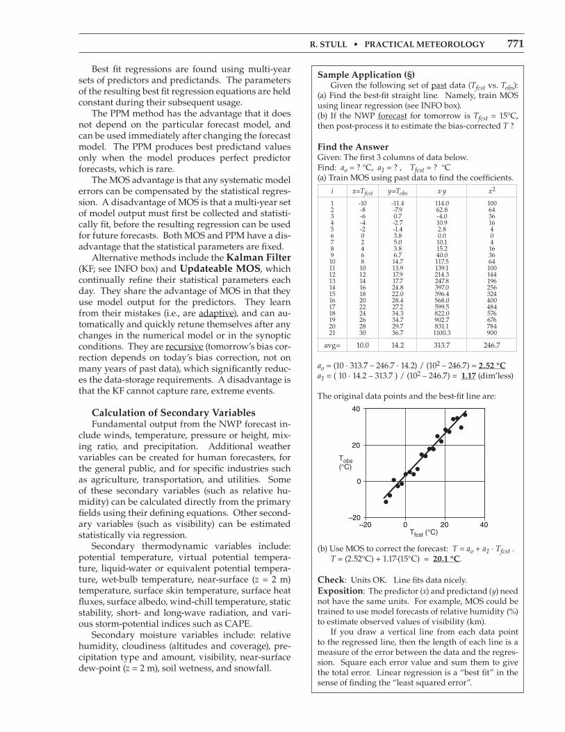
r. Stull • Practical meteorology 771
Best fit regressions are found using multi-year sets of predictors and predictands. The parameters of the resulting best fit regression equations are held constant during their subsequent usage. The PPM method has the advantage that it does not depend on the particular forecast model, and can be used immediately after changing the forecast model. The PPM produces best predictand values only when the model produces perfect predictor forecasts, which is rare. The MOS advantage is that any systematic model errors can be compensated by the statistical regres-sion. A disadvantage of MOS is that a multi-year set of model output must first be collected and statisti-cally fit, before the resulting regression can be used for future forecasts. Both MOS and PPM have a dis-advantage that the statistical parameters are fixed. Alternative methods include the Kalman Filter (KF; see INFO box) and updateable moS, which continually refine their statistical parameters each day. They share the advantage of MOS in that they use model output for the predictors. They learn from their mistakes (i.e., are adaptive), and can au-tomatically and quickly retune themselves after any changes in the numerical model or in the synoptic conditions. They are recursive (tomorrow’s bias cor-rection depends on today’s bias correction, not on many years of past data), which significantly reduc-es the data-storage requirements. A disadvantage is that the KF cannot capture rare, extreme events.
calculation of Secondary Variables Fundamental output from the NWP forecast in-clude winds, temperature, pressure or height, mix-ing ratio, and precipitation. Additional weather variables can be created for human forecasters, for the general public, and for specific industries such as agriculture, transportation, and utilities. Some of these secondary variables (such as relative hu-midity) can be calculated directly from the primary fields using their defining equations. Other second-ary variables (such as visibility) can be estimated statistically via regression. Secondary thermodynamic variables include: potential temperature, virtual potential tempera-ture, liquid-water or equivalent potential tempera-ture, wet-bulb temperature, near-surface (z = 2 m) temperature, surface skin temperature, surface heat fluxes, surface albedo, wind-chill temperature, static stability, short- and long-wave radiation, and vari-ous storm-potential indices such as CAPE. Secondary moisture variables include: relative humidity, cloudiness (altitudes and coverage), pre-cipitation type and amount, visibility, near-surface dew-point (z = 2 m), soil wetness, and snowfall.
Sample application (§) Given the following set of past data (Tfcst vs. Tobs): (a) Find the best-fit straight line. Namely, train MOS using linear regression (see INFO box). (b) If the NWP forecast for tomorrow is Tfcst = 15°C, then post-process it to estimate the bias-corrected T ?
Find the answerGiven: The first 3 columns of data below.Find: ao = ? °C, a1 = ? , Tfcst = ? °C(a) Train MOS using past data to find the coefficients.
i x=Tfcst y=Tobs x·y x2
123456789101112131415161718192021
-10-8-6-4-2024681012141618202224262830
-11.4-7.90.7-2.7-1.43.85.03.86.714.713.917.917.724.822.028.427.234.334.729.736.7
114.062.8-4.010.92.80.010.115.240.0117.5139.1214.3247.8397.0396.4568.0599.5822.0902.7831.1
1100.3
100643616404163664100144196256324400484576676784900
avg= 10.0 14.2 313.7 246.7
ao = (10 · 313.7 – 246.7 · 14.2) / (102 – 246.7) = 2.52 °c a1 = ( 10 · 14.2 – 313.7 ) / (102 – 246.7) = 1.17 (dim’less)
The original data points and the best-fit line are:
(b) Use MOS to correct the forecast: T = ao + a1 · Tfcst . T = (2.52°C) + 1.17·(15°C) = 20.1 °c.
check: Units OK. Line fits data nicely.exposition: The predictor (x) and predictand (y) need not have the same units. For example, MOS could be trained to use model forecasts of relative humidity (%) to estimate observed values of visibility (km). If you draw a vertical line from each data point to the regressed line, then the length of each line is a measure of the error between the data and the regres-sion. Square each error value and sum them to give the total error. Linear regression is a “best fit” in the sense of finding the “least squared error”.

772 chaPter 20 • Numerical Weather PredictioN (NWP)
Secondary dynamic variables include stream-lines, trajectories, absolute vorticity, potential vorticity, isentropic potential vorticity, dynamic tropopause height, vorticity advection, Richardson number, dynamic stability, near-surface winds (z = 10 m), surface stress, surface roughness, mean-sea-level pressure, and turbulence. While many of the above variables are computed at central numerical-computing facilities, additional computations can be made by separate organiza-tions. Local forecast offices of National Weather Ser-vices can tailor the numerical guidance to produce local forecasts of maximum and minimum tempera-ture, precipitation, cloudiness, and storm and flood warnings for the neighboring counties. Consulting firms, broadcast companies, utility companies, and airlines, for example, acquire the fundamental and secondary fields via data networks such as the internet. From these fields they compute products such as computerized flight plans for air-craft, crop indices and threats such as frost, hours of sunshine, and heating- or cooling-degree days for energy consumption. Universities also acquire the primary and sec-ondary output fields, to use for teaching and re-search. Some of the applications result in weather maps that are put back on the internet.
Weather maps and other graphics The fundamental and secondary variables that are output from the NWP and from forecast refine-ment are arrays of numbers. To make these data easier to use and interpret by humans, the numbers can be converted into weather-map graphics and an-imations, meteograms (plots of a weather variable vs. time), sounding profiles, cross-sections, text fore-casts, and other output forms. Computation of these outputs can take hours, depending on the graphical complexity and the number of products, and thus cannot be neglected in the forecast schedule. Some visualization programs for NWP output include: GrADS, Vis5D, MatLab, NCAR RIP, GEM-PAK, unidata IDV, AWIPS, and NinJo.
compression into databases and clima-tologies
It is costly to save the terabytes of output pro-duced by operational NWP models every day for every grid point, every level, and every time step. Instead, only key weather fields at RAOB mandato-ry levels in the atmosphere are saved. These WMO standard isobaric surfaces are: surface, 100, 92.5, 85, 70, 50, 40, 30, 25, 20, 15, 10, 7, 5, 3, 2, & 1 kPa. Output files can be converted from model-specific formats to standard formats (NetCDF, Vis5D, SQL, GRIB). Forecasts at key locations such as weather stations can be accumulated into growing climatologies.
Sample application Given the following simplified MOS regression:
Tmin = –295 + 0.4 · T15 + 0.25 · ∆TH + 0.6 · Td
for daily minimum temperature (K) in winter at Madi-son, Wisconsin, where T15 = observed surface tem-perature (K) at 15 UTC, ∆TH = model forecast of 100-85 kPa thickness (m), and Td = model fcst. dew point (K). Predict Tmin given NWP model forecasts of: T15 = 273 K, ∆TH = 1,200 m, and Td = 260 K.
Find the answerGiven: T15 = 273 K, ∆TH = 1,200 m, and Td = 260 K.Find: Tmin = ? K
Tmin = –295 + 0.4·(273) + 0.25·(1,200)+ 0.6·(260) = 270.2 ≈ –3°c.
check: Units OK. Physics OK.exposition: Chilly, but typical for winter in Madison. Note that MOS regressions can be made for any vari-ables in any units. Thus, (1) units might not be consis-tent from term to term in the regression, but (2) you MUST use the same units for each variable as was used when the MOS regression was created.
info • Human contributions
NWP forecasts are rarely perfect. Thus, humans have the opportunity to improve the forecasts. By comparing the current model forecast to recent observations, you can discover biases early in the fore-cast that you can use to correct future forecasts. For example, if the NWP forecast for your location was 2 °C too cold during the past few hours, perhaps it will continue to be 2 °C too cold in the next few hours. Er-rors in timing or position of fronts and cyclones early in the forecast can be extrapolated to anticipate what corrections are needed for wind and precipitation forecasts later. You can incorporate knowledge of local effects that might not be resolved by the model — such as the effects of local terrain, coastlines, land use, and urban centers. You may have noticed that some NWP models do not perform well in certain weather pat-terns, so you can anticipate similar errors when those same weather patterns happen in the future. Humans can also tailor the weather forecasts to in-dividual users and industries. Examples are forecasts for road or rail transportation, aviation, shipping/fishing/recreational boating, servicing of offshore oil platforms, electrical utility companies (including hydro and wind-energy), air-quality regulatory agen-cies, avalanche forecast centers, flood and landslide prediction, forest-fire fighting, ski resorts, emergency services, etc. Humans are also rarely perfect. Nonetheless, stud-ies have shown that the best forecasts are achieved by
a combination of NWP and human experience.

r. Stull • Practical meteorology 773
nonLinear DynaMicS anD cHaoS
Predictability Recall that NWP is an initial-value problem, where these initial values are partially based on ob-served weather conditions. Unfortunately, the ob-servations include instrumentation, sampling, and representativeness errors. We have already exam-ined how such errors cause startup problems due to imbalanced flow conditions. How do these errors affect the long-range predictability? Lorenz suggested that the equations of motion (which are nonlinear because they contain products of dependent variables, such as U and T in U·∆T/∆x) are sensitive to initial conditions. Such sensitiv-ity means that small differences in initial conditions can grow into large differences in the forecasts. This is unfortunate. Initial conditions will always have errors. Thus our forecasts will always become less accurate with increasing forecast time. Thus, there is a limit to the predictability of weather that is related to instability of the dynamics. A simple physical illustration of sensitive de-pendence to initial conditions is a toy balloon. Inflate one with air and then let it go to fly around the room. Repeat the experiment, being careful to inflate the balloon the same amount and to point it in the same direction. You probably know from ex-perience that the path and final destination of the balloon will differ greatly from flight to flight. In spite of how simple a toy balloon seems, the dy-namical equations describing its flight are extremely sensitive to initial conditions, making predictions of flight path virtually impossible.
Lorenz Strange attractor Another illustration of sensitive dependence to initial conditions was suggested by Lorenz. Sup-pose we examine 2-D convection within a tank of water, where the bottom of the tank is heated (Fig. 20.16). The vertical temperature gradient from bot-tom to top drives a circulation of the water, with warm fluid trying to rise. The circulation can mod-ify the temperature distribution within the tank. A very specialized, highly-simplified set of equa-tions that approximates this flow is:
∆∆
= −
∆∆
= − −
∆∆
= −
Ct
L C
Lt
r C L C M
Mt
C L b M
σ ·( )
· ·
· ·
(20.23)
a Scientific PerSPectiVe • Scientific revolutions
In the late 1950s and early 1960s, Ed Lorenz was making numerical forecasts of convection to deter-mine if statistical forecasts were better than NWP forecasts using the nonlinear dynamical equations. One day he re-ran a numerical forecast, but entered slightly different initial data. He got a strikingly dif-ferent answer. He was curious about this effect, and allowed himself to become sidetracked from his original in-vestigations. This lead to his description of chaos, discovery of a strange attractor, and realization of the sensitive dependence of some equations to initial con-ditions. He published his results in 1963 (“Deterministic non-periodic flow”. J. Atmos. Sci., 20, p 130-141). From 1963 to about 1975, this innovative paper was rarely cited by other scientists — a clue that it was not yet accepted by his colleagues. However, between 1975 to 1980, researchers were becoming increasingly aware of his work. From 1980 to present, this paper has been cited on the order of 100 times per year. About a decade and a half elapsed before this new theory gained wide acceptance, which is typical of many paradigm shifts. Namely, it takes about one human generation for a scientific revolution to ma-ture, because typically the older scientists (who hold the power) are not willing to make the shift. The sci-entific revolution occurs when this group retires and younger scientists (with the newer ideas) take their place.
Figure 20.16Tank of fluid (shaded), showing circulation C. The vertical M and horizontal L distributions of temperature are also shown.
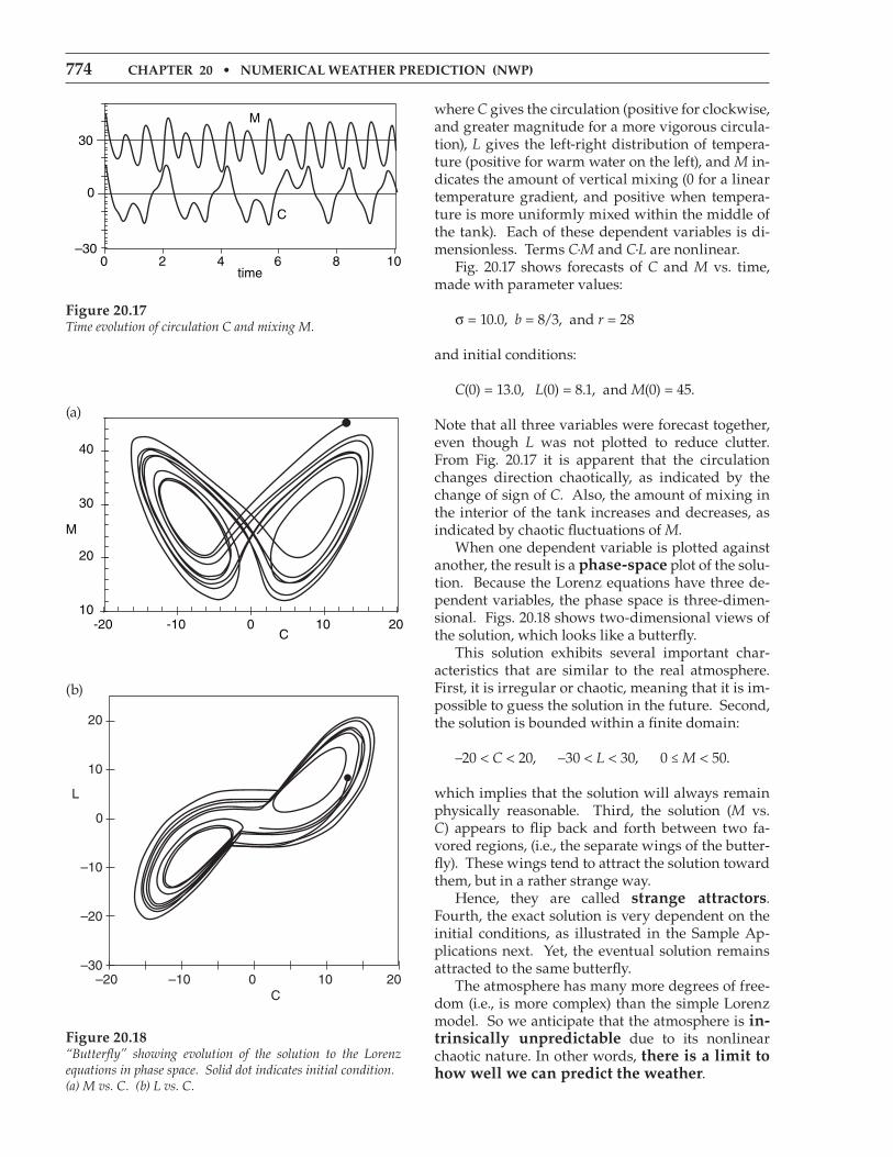
774 chaPter 20 • Numerical Weather PredictioN (NWP)
where C gives the circulation (positive for clockwise, and greater magnitude for a more vigorous circula-tion), L gives the left-right distribution of tempera-ture (positive for warm water on the left), and M in-dicates the amount of vertical mixing (0 for a linear temperature gradient, and positive when tempera-ture is more uniformly mixed within the middle of the tank). Each of these dependent variables is di-mensionless. Terms C·M and C·L are nonlinear. Fig. 20.17 shows forecasts of C and M vs. time, made with parameter values:
σ = 10.0, b = 8/3, and r = 28
and initial conditions:
C(0) = 13.0, L(0) = 8.1, and M(0) = 45.
Note that all three variables were forecast together, even though L was not plotted to reduce clutter. From Fig. 20.17 it is apparent that the circulation changes direction chaotically, as indicated by the change of sign of C. Also, the amount of mixing in the interior of the tank increases and decreases, as indicated by chaotic fluctuations of M. When one dependent variable is plotted against another, the result is a phase-space plot of the solu-tion. Because the Lorenz equations have three de-pendent variables, the phase space is three-dimen-sional. Figs. 20.18 shows two-dimensional views of the solution, which looks like a butterfly. This solution exhibits several important char-acteristics that are similar to the real atmosphere. First, it is irregular or chaotic, meaning that it is im-possible to guess the solution in the future. Second, the solution is bounded within a finite domain:
–20 < C < 20, –30 < L < 30, 0 ≤ M < 50.
which implies that the solution will always remain physically reasonable. Third, the solution (M vs. C) appears to flip back and forth between two fa-vored regions, (i.e., the separate wings of the butter-fly). These wings tend to attract the solution toward them, but in a rather strange way. Hence, they are called strange attractors. Fourth, the exact solution is very dependent on the initial conditions, as illustrated in the Sample Ap-plications next. Yet, the eventual solution remains attracted to the same butterfly. The atmosphere has many more degrees of free-dom (i.e., is more complex) than the simple Lorenz model. So we anticipate that the atmosphere is in-trinsically unpredictable due to its nonlinear chaotic nature. In other words, there is a limit to how well we can predict the weather.
Figure 20.17Time evolution of circulation C and mixing M.
Figure 20.18“Butterfly” showing evolution of the solution to the Lorenz equations in phase space. Solid dot indicates initial condition.(a) M vs. C. (b) L vs. C.
(a)
(b)

r. Stull • Practical meteorology 775
Science graffiti
Sensitive dependence on initial conditions
“Does the flap of a butterfly’s wings in Brazil set off a tornado in Texas?” – E. Lorenz & P. Merilees, 1972.
“Can a man sneezing in China cause a snow storm in New York? – George R. Stewart, 1941: Storm.
“Did the death of a prehistoric butterfly change the outcome of a US presidential election?” – Ray Brad-bury, 1952, 1980, A Sound of Thunder.
Sample application (§) Solve the Lorenz equations for the parameters and initial conditions listed previously in this chapter. Use a dimensionless time step of ∆t = 0.01, and forecast from t = 0 to t = 10.
Find the answerGiven: C(0) = 13.0, L(0) = 8.1, and M(0) = 45, and σ = 10.0, b = 8/3, and r = 28.Find: C(t) = ?, L(t) = ?, M(t) = ?
First, rewrite eqs. (20.23) in the form of a forecast:
C t t C t t L t C t
L t T L t
( ) ( ) ·[ ·( ( ) ( ))]
( ) ( )
+ ∆ = + ∆ −
+ ∆ =
σ
++ ∆ − −
+ ∆ = + ∆
t r C t L t C t M t
M t T M t t
·[ · ( ) ( ) ( )· ( )]
( ) ( ) ··[ ( )· ( ) · ( )]C t L t b M t−
As an example, for the 1st step: C(0.01) = 13.0 + 0.01·[10.0·(8.1-13.0)] = 12.51Next, set this up on a spreadsheet, a portion of which is reproduced below. t C L M .0.00 13.00 8.1 45.000.01 12.51 5.809 44.850.02 11.84 3.643 44.380.03 11.02 1.666 43.630.04 10.08 -0.07 42.650.05 9.069 -1.55 41.510.06 8.007 -2.76 40.260.07 6.931 -3.71 38.960.08 5.866 -4.44 37.670.09 4.836 -4.96 36.40.10 3.856 -5.32 35.19Note that your answers might be different than these, due to different round-off errors and mathematical li-braries on the spreadsheets. Plots. These answers are already plotted in Figs. 20.17 - 20.18.
check: Units dimensionless. Physics OK.exposition: The forecast equations above use an Euler time-differencing scheme, which is the least ac-curate. Nevertheless, it illustrates the Lorenz attractor.
Sample application (§) Repeat the previous Sample Application, but for a slightly different initial condition: M(0) = 44.
Find the answerGiven: C(0) = 13.0, L(0) = 8.1, and M(0) = 44, and σ = 10.0, b = 8/3, r = 28.Find: C(t) = ?, L(t) = ?, M(t) = ?
As in the previous Sample Application.
check: Units OK. Physics OK.exposition: These are quite different from Figs. 20.17 & 20.18, demonstrating sensitive dependence to initial conditions.
Science graffito
“Computations indicate that a perfect model should produce:• three-day forecasts ... which are generally good; • one-week forecasts ... which are occasionally good; • and two-week forecasts ... which, although not very good, may contain some useful information” – E. Lorenz, 1993: The Essence of Chaos.
Univ. of Washington Press, Seattle. 227 pp.

776 chaPter 20 • Numerical Weather PredictioN (NWP)
ensemble forecasts Some forecast centers repeatedly forecast the same time period, but for different conditions. These differences can be created by using different initial conditions, physical parameterizations, numerics, and/or NWP models. Such a procedure yields an ensemble of forecasts, which reveal the sensitive dependence of weather forecasts on those different conditions. Fig. 20.19 shows 10-day ensemble fore-casts of 85-kPa temperature, precipitation, and 50-kPa geopotential heights at Des Moines, Iowa, for the same case-study period as discussed previously. The heavy dotted line in these figures shows the single forecast run made with the high-resolution model, starting from the “best” initial conditions. This is the “official” forecast produced by ECMWF. The thick solid line starts from the same initial con-ditions, but is made with a coarser grid resolution to save forecast time. Note that the forecast changes substantially when the grid resolution changes. The thin lines are forecasts from slightly differ-ent initial conditions. To save computer time, these multiple forecasts are also made with the lower grid-resolution. The forecasts of temperature and geopotential height start out quite close, and diverge slowly during the first 3.5 days. At that time (rough-ly when the cyclone reaches Des Moines late 22 Feb 94), the solution rapidly diverges, signaling a sudden loss in forecast skill that is never regained. The spread of the ensemble members informs you about the uncertainty of the forecast. Unfor-tunately, you have no way of knowing which of the ensemble members will be closest to reality. By averaging all the ensemble members together, you can find an ensemble average forecast that is usually more skillful than any individual member. This is one of the strengths of ensemble forecasting. After several days into the forecast (Fig. 20.19), the ensemble forecasts seem chaotic. Yet this chaotic so-lution is bounded within a finite region — perhaps a “strange attractor” such as studied by Lorenz. Studies of chaos often focus on the eventual state of the solution, at times far from the initial condi-tion. At these long times, the dynamics have forgot-ten the initial state. Although this eventual state is somewhat useless as a weather forecast, it can pro-vide some insight into the range of possible climatic conditions that are allowed by the dynamical equa-tions in the model (i.e., the model’s climate). Ensemble forecasts can also suggest which con-ditions are unlikely — valuable information for some users. For example, if none of the ensemble forecasts give temperatures below freezing on a par-ticular day, then a categorical “no freeze” forecast could be made. Better confidence in such forecasts is possible by calibrating the ensemble spread into a probabilistic forecast, discussed next.
Figure 20.19Ten-day ensemble forecasts for Des Moines, Iowa, starting from 19 Feb 1994. (a) Temperature (°C) at 85 kPa. (b) Total precipi-tation (mm). (c) Geopotential height (km) of the 50 kPa surface. Thick solid line is a coarse-resolution forecast that was started from the analyzed initial conditions. Thin lines are course-resolution forecasts, each started from a slightly different initial condition created by adding a different small perturbation to the analysis. The thick dotted line shows a single high-resolution forecast started from the analyzed initial conditions. (Courtesy of ECMWF, 1999).
(c) Geopotential Height (km)
(b) Total Precipitation (mm)
(a) Temperature (°C)
0 1 2 3 4 5 6 7 8 9 10 Forecast Day
10
0
–10
–20
20.
15.
10.
5.
0.
5.6
5.5
5.4
5.3

r. Stull • Practical meteorology 777
Probabilistic forecasts Due to the inherent unpredictability of the atmo-sphere, we cannot confidently make deterministic forecasts such as “the temperature tomorrow at noon will be exactly 19.0°C”. However, it is possible to routinely create probabilistic forecasts similar to “there is a 60% chance the temperature tomorrow at noon will be between 17°C and 21°C, and an 80% chance the it will be between 14 and 24°C.” Ensemble forecasts are increasingly used to cre-ate probabilistic forecasts. Various methods can be used to convert the distribution of ensemble mem-bers into calibrated probabilistic forecasts, such as illustrated in Fig. 20.20. The spread of the probability distribution (i.e., the uncertainty in the forecast) depends on the sea-son (greater spread in winter), the location (greater spread downwind of data-void regions), the climate (greater spread in parts of the globe where weather is more variable), and on the accuracy of the NWP models. A perfect forecast would have no spread. Often probability forecasts are given as a cumu-lative probability CP that some threshold will be met. In Fig. 20.20, the lowest solid line represents a cumulative probability of CP = 10% (there is a 10% chance that the observed temperature will be colder than this forecast temperature) and the highest solid black line is for CP = 90% (there is a 90% chance that the observation will be colder than this forecast). For example, using Fig. 20.20 we could tell a farm-er that there is 35% chance the low temperature will be below freezing (Tthreshold = 0°C) on 6 - 7 Jan 2011.
forecaSt quaLity & Verification
NWP forecasts can have both systematic error and random error (see Appendix A). By making ensemble forecasts you can reduce random errors caused by the chaotic nature of the atmosphere. By postprocessing each ensemble member using Model Output Statistics, you can reduce systematic errors (biases) before computing the ensemble average. After making these corrections, the forecast is still not perfect. How good is the forecast? Verification is the process of determining the quality of a forecast. Quality can be measured in different ways, using various statistical definitions. One of the least useful measures of quality is fore-cast accuracy. For example, in Vancouver, Canada, clouds are observed 327 days per year, on average. If I forecast clouds every day of the year, then my accuracy (= number of correct forecasts / total num-ber of forecasts) will be 327/365 = 90% on the aver-age. Although this accuracy is quite high, it shows no skill. To be skillful, I must beat climatology to successfully forecast which days will be cloudless. Skill measures forecast improvement above some reference such as the climatic average, persis-tence, or a random guess. On some days the forecast is better than others, so these measures of skill are usually averaged over a long time (months to years) and over a large area (such as all the grid points in the USA, Canada, Europe, or the world). Methods to calculate verification scores and skills for various types of forecasts are presented next.
continuous Variables An example of a continuous variable is tempera-ture, which varies over a wide range of values. Oth-er variables are bounded continuous. For example, precipitation is bounded on one side — it cannot be less than zero. Relative humidity is bounded on two sides — it cannot be below 0% nor greater than 100%, but otherwise can vary smoothly in between. First, define the terms. Let: A = initial analysis (based on observations) V = verifying analysis (based on later obs.) F = deterministic forecast C = climatological conditions n = number of grid points being averaged
An anomaly is defined as the difference from climatology at any instant in time. For example F – C = predicted anomaly A – C = persistence anomaly V – C = verifying anomaly
Figure 20.20Calibrated probabilistic forecast for the minimum temperature (Tmin °C) at Vancouver Airport (CYVR) for 2 to 17 Jan 2011. The thin white line surrounded by black is the median (50% of the observations should fall below this line, and 50% above). The black, dark grey, medium grey, and light grey regions span ±10%, 20%, 30%, and 40% of cumulative probability around the median. The dashed lines are ±49% around the median — namely, 98% of the time the observations should fall between the dashed lines. The dots are the raw forecasts from each of the 42 members of the North American Ensemble Forecast System.
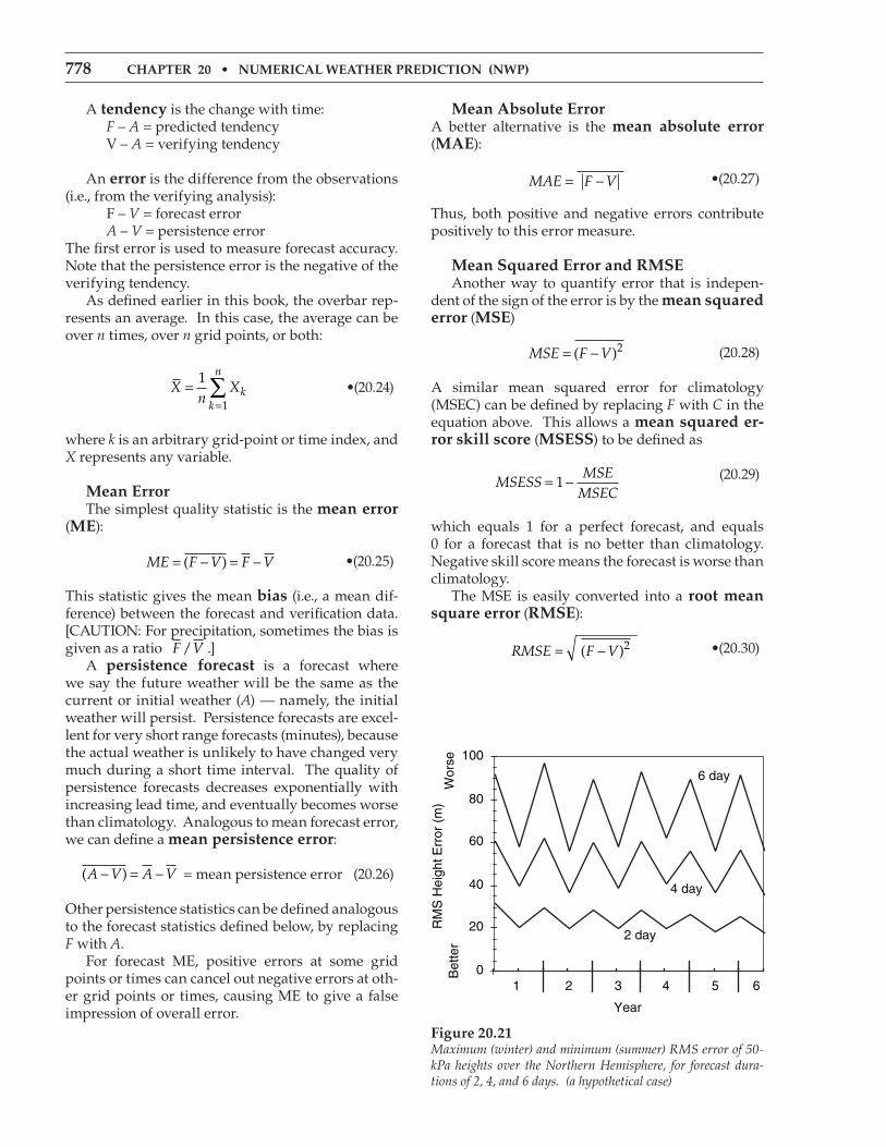
778 chaPter 20 • Numerical Weather PredictioN (NWP)
A tendency is the change with time: F – A = predicted tendency V – A = verifying tendency
An error is the difference from the observations (i.e., from the verifying analysis): F – V = forecast error A – V = persistence errorThe first error is used to measure forecast accuracy. Note that the persistence error is the negative of the verifying tendency. As defined earlier in this book, the overbar rep-resents an average. In this case, the average can be over n times, over n grid points, or both:
Xn
Xkk
n=
=∑1
1 •(20.24)
where k is an arbitrary grid-point or time index, and X represents any variable.
mean error The simplest quality statistic is the mean error (me):
ME F V F V= − = −( ) •(20.25)
This statistic gives the mean bias (i.e., a mean dif-ference) between the forecast and verification data. [CAUTION: For precipitation, sometimes the bias is given as a ratio Precip.Bias = F V/ .] A persistence forecast is a forecast where we say the future weather will be the same as the current or initial weather (A) — namely, the initial weather will persist. Persistence forecasts are excel-lent for very short range forecasts (minutes), because the actual weather is unlikely to have changed very much during a short time interval. The quality of persistence forecasts decreases exponentially with increasing lead time, and eventually becomes worse than climatology. Analogous to mean forecast error, we can define a mean persistence error:
( )A V A V− = − = mean persistence error (20.26)
Other persistence statistics can be defined analogous to the forecast statistics defined below, by replacing F with A. For forecast ME, positive errors at some grid points or times can cancel out negative errors at oth-er grid points or times, causing ME to give a false impression of overall error.
mean absolute errorA better alternative is the mean absolute error (mae):
MAE F V= − •(20.27)
Thus, both positive and negative errors contribute positively to this error measure.
mean Squared error and rmSe Another way to quantify error that is indepen-dent of the sign of the error is by the mean squared error (mSe)
MSE F V= −( )2 (20.28)
A similar mean squared error for climatology (MSEC) can be defined by replacing F with C in the equation above. This allows a mean squared er-ror skill score (mSeSS) to be defined as
MSESSMSE
MSEC= −1 (20.29)
which equals 1 for a perfect forecast, and equals 0 for a forecast that is no better than climatology. Negative skill score means the forecast is worse than climatology. The MSE is easily converted into a root mean square error (rmSe):
RMSE F V= −( )2 •(20.30)
Figure 20.21Maximum (winter) and minimum (summer) RMS error of 50-kPa heights over the Northern Hemisphere, for forecast dura-tions of 2, 4, and 6 days. (a hypothetical case)

r. Stull • Practical meteorology 779
This statistic not only includes contributions from each individual grid point or time, but it also in-cludes any mean bias error. RMSE increases with forecast duration (i.e., lead time, or forecast range). It is also greater in winter than summer, because summer usually has more quiescent weather. Fig. 20.21 shows the maximum (winter) and minimum (summer) RMS errors of the 50 kPa heights in the Northern Hemisphere, for hy-pothetical forecasts.
correlation coefficient To discover how well the forecast and verifica-tion vary together (e.g., hotter than average on the same days, colder than average on the same days), you can use the Pearson product-moment correla-tion coefficient, r:
rF V
F V= ' '
( ') · ( ')2 2 •(20.31)
where
F F F' = − and V V V' = − (20.32)
The correlation coefficient is in the range –1 ≤ r ≤ 1. It varies from +1 when the forecast varies perfectly with the verification (e.g., forecast hot when verifi-cation hot), to –1 for perfect opposite variation (e.g., forecast hot when verification cold), and is zero for no common variation.
anomaly correlation anomaly correlations indicate whether the forecast (or persistence) is varying from climatol-ogy in the same direction as the observations. For example, if the forecast is for warmer-than-normal temperatures and the verification confirms that warmer-than-normal temperatures were observed, then there is a positive correlation between the fore-cast and the weather. At other grid points where the forecast is poor, there might be a negative correla-tion. When averaged over all grid points, one hopes that there are more positive than negative correla-tions, giving a net positive correlation. By dividing the correlations by the standard de-viations of forecast and verification anomalies, the result is normalized into an anomaly correlation coefficient. This coefficient varies between 1 for a perfect forecast, to 0 for an awful forecast. (Actually, for a really awful forecast the correlation can reach a minimum of –1, which indicates that the forecast is opposite to the weather. Namely, the model fore-casts warmer-than-average weather when colder weather actually occurs, and vice-versa.)
Sample application (§) Given the following synthetic analysis (A), NWP forecast (F), verification (V), and climate (C) fields of 50-kPa height (km). Each field represents a weather map (North at top, East at right).
Analysis: 5.3 5.3 5.3 5.4 5.4 5.3 5.4 5.5 5.5 5.4 5.5 5.6 5.6 5.5 5.6 5.7 5.7 5.6 5.7 5.7Forecast: 5.5 5.2 5.2 5.3 5.6 5.4 5.3 5.4 5.6 5.5 5.4 5.5 5.7 5.6 5.5 5.6 5.7 5.7 5.6 5.6Verification: 5.4 5.3 5.3 5.3 5.5 5.4 5.3 5.4 5.5 5.5 5.4 5.5 5.6 5.6 5.5 5.6 5.6 5.7 5.6 5.7Climate: 5.4 5.4 5.4 5.4 5.4 5.4 5.4 5.4 5.5 5.5 5.5 5.5 5.6 5.6 5.6 5.6 5.7 5.7 5.7 5.7
Find the mean error of the forecast and of persis-tence. Find the forecast MAE and MSE. Find MSEC and MSESS. Find the correlation coefficient between the forecast and verification. Find the RMS errors and the anomaly correlations for the forecast and persis-tence.
Find the answerUse eq. (20.25): MEforecast = 0.01 km = 10 m Use eq. (20.26): MEpersistence = 15 m Use eq. (20.27): MAE = 40 m Use eq. (20.28): MSEforecast = 0.004 km2 = 4000 m2 Use eq. (20.28): MSEC = 0.0044 km2 = 4500 m2 Use eq. (20.29): MSESS = 1 – (4000/4500) = 0.11 Use eq. (20.30): RMSEforecast = 63 m Use eq. (20.30): RMSEpersistence = 87 m Use eq. (20.31): r = 0.92 (dimensionless)Use eq. (20.33): forecast anomaly correlation = 81.3% Use eq. (20.34): persist. anomaly correlation = 7.7%
check: Units OK. Physics OK.exposition: Analyze (i.e., draw height contour maps for) the analysis, forecast, verification, and climate fields. The analysis shows a Rossby wave with ridge and trough, and the verification shows this wave mov-ing east. The forecast amplifies the wave too much. The climate field just shows the average of higher heights to the south and lower heights to the north, with all transient Rossby waves averaged out.

780 chaPter 20 • Numerical Weather PredictioN (NWP)
The definitions of these coefficients are:
anomaly correlation coef. for the forecast =
( ) ( ) · ( ) ( )
( ) ( )
F C F C V C V C
F C F C
− − − − − −
− − − − − − 2 2
· ( ) ( )V C V C (20.33)
anomaly correlation coef. for persistence =
( ) ( ) · ( ) ( )
( ) ( )
A C A C V C V C
A C A C
− − − − − −
− − − − − − 2 2
· ( ) ( )V C V C (20.34)
Fig. 20.22 compares hypothetical persistence and NWP-forecast anomaly correlations for 50-kPa geopotential height. One measure of forecast skill is the vertical separation between the forecast and persistence curves in Fig. 20.22. This figure shows that the forecast beats persis-tence over the full 10 days of forecast. Also, using 60% correlation as an arbitrary measure of quality, we see that a “good” persistence forecast extends out to only about 2 days, while a “good” NWP forecast is obtained out to about 6 days, for this hypotheti-cal case for 50 kPa geopotential heights. For other weather elements such as precipitation or surface temperature, both solid curves decrease more rap-idly toward climatology.
Binary / categorical events A binary event is a yes/no event, such as snow or no snow. Continuous variables can be converted into binary variables by using a threshold. For ex-ample, is the temperature below freezing (0°C) or not? Does precipitation exceed 25 mm or not? A contingency table (Fig. 20.23a) has cells for each possible outcome of forecast and observation. “Hit” means the event was successfully forecast. “Miss” means it occurred but was not forecast. “False Alarm” means it was forecast but did not happen. “Correct Rejection” means that the event was correctly forecast not to occur. After making a series of categorical forecasts, the forecast outcomes can be counted into each cell of a contingency table. Let a, b, c, d represent the counts of all occurrences as shown in Fig. 20.23b. The total number of forecasts is n:
n = a + b + c + d (20.35)
Figure 20.23Contingency table for a binary (Yes/No) situation. “Yes” means the event occurred or was forecast to occur. (a) Meaning of cells. (b) Counts of occurrences, where a + b + c + d = n. (c) Expense matrix, where C = cost for taking protective action (i.e., for miti-gating the loss), and L = loss due to an unmitigated event.
Figure 20.22NWP forecast skill (thick line) of 50-kPa heights for a hypotheti-cal forecast model. A persistence forecast (thin line) is one where the weather is assumed not to change with time from the initial conditions. A value of 100% is a perfect forecast, while a value of 0 is no better than climatology (dotted line).

r. Stull • Practical meteorology 781
The bias score B indicates over- or under-pre-diction of the frequency of event occurrence:
Ba ba c
= ++
(20.36)
The portion correct PC (also known as portion of forecasts correct PFC) is
PCa d
n= +
(20.37)
But perhaps a portion of PC could have been due to random-chance (dumb but lucky) forecasts. Let E be this “random luck” portion, assuming that you made the same ratio of “YES” to “NO” forecasts:
Ea b
na c
nd b
nd c
n= +
+
+ +
+
· · (20.38)
We can now define the portion of correct forecasts that was actually skillful (i.e., not random chance), which is known as the heidke skill score (HSS):
HSSPC E
E= −
−1 (20.39)
The hit rate H is the portion of actual occurrenc-es (obs. = “YES”) that were successfully forecast:
Ha
a c=
+ •(20.40)
It is also known as the probability of detection POD. The false-alarm rate F is the portion of non-occurrences (observation = “NO”) that were incor-rectly forecast:
Fb
b d=
+ •(20.41)
Don’t confuse this with the false-alarm ratio FAR, which is the portion of “YES” forecasts that were wrong: FAR
ba b
=+
(20.42)
A true skill score TSS (also known as Peirce’s skill score PSS, and as hansen and Kuipers’ score) can be defined as
TSS H F= − (20.43)
which is a measure of how well you can discrimi-nate between an event and a non-event, or a mea-sure of how well you can detect an event. A critical success index CSI (also known as a threat score TS) is:
CSIa
a b c=
+ + (20.44)
Sample application Given the following contingency table, calculate all the binary verification statistics. Observation Yes NoForecast Yes: 90 50 No 75 150
Find the answer:Given: a = 90 , b = 50 , c = 75 , d = 150Find: B, PC, HSS, H, F, FAR, TSS, CSI, GSS
First, use eq. (20.35): n = 90 + 50 + 75 + 150 = 365So apparently we have daily observations for a year.
Use eq. (20.36): B = (90 + 50) / (90 + 75) = 0.85 Use eq. (20.37): PC = (90 + 150) / 365 = 0.66 Use eq. (20.38): E = [(90+50)·(90+75) + (150+50)·(150+75)]/(3652) E = 68100 / 133225 = 0.51 Use eq. (20.39): HSS = (0.66 – 0.51) / (1 – 0.51) = 0.31 Use eq. (20.40): H = 90 / (90 + 75) = 0.55 Use eq. (20.41): F = 50 / (50 + 150) = 0.25 Use eq. (20.42): FAR = 50 / (90 + 50) = 0.36 Use eq. (20.43): TSS = 0.55 – 0.25 = 0.30 Use eq. (20.44): CSI = 90 / (90 + 50 + 75) = 0.42 Use eq. (20.45): ar = [ (90+50)·(90+75)]/365 = 63.3 Use eq. (20.46): GSS = (90–63.3) / (90–63.3+50+75) = 0.18
check: Values reasonable. Most are dimensionless.exposition: No verification statistic can tell you whether the forecast was “good enough”. That is a subjective decision to be made by the end user. One way to evaluate “good enough” is via a cost/loss mod-el (see next section).

782 chaPter 20 • Numerical Weather PredictioN (NWP)
which is the portion of hits given that the event was forecast, or observed, or both. This is often used as a forecast-quality measure for rare events. Suppose we consider the portion of hits that might have occurred by random chance ar:
aa b a c
nr =+ +( )·( )
(20.45)
Then we can subtract this from the actual hit count to modify CSS into an equitable threat score ETS, also known as gilbert’s skill score GSS:
GSSa a
a a b cr
r= −
− + + (20.46)
which is also useful for rare events. For a perfect forecasts (where b = c = 0), the values of these scores are: B = 1, PC = 1, HSS = 1, H = 1, F = 0, FAR = 0, TSS = 1, CSI = 1, GSS = 1. For totally wrong forecasts (where a = d = 0): B = 0 to ∞, PC = 0, HSS = negative, H = 0, F = 1, FAR = 1, TSS = –1, CSI = 0, GSS = negative.
Probabilistic forecasts
Brier Skill Score For calibrated probability forecasts, a Brier skill score (BSS) can be defined relative to climatology as
BSS
p o
o N o
k kk
N
kk
N
kk
N= −
−
−
=
= =
∑
∑ ∑1
2
1
1 1
( )
·
•(20.47)
where pk is the forecast probability (0 ≤ pk ≤ 1) that the threshold will be exceeded (e.g., the probabil-ity that the precipitation will exceed a precipitation threshold) for any one forecast k, and N is the num-ber of forecasts. The verifying observation ok = 1 if the observation exceeded the threshold, and is set to zero otherwise. BSS = 0 for a forecast no better than climatology. BSS = 1 for a perfect deterministic forecast (i.e., the forecast is pk = 1 every time the event happens, and pk = 0 every time it does not). For probabilistic fore-casts, 0 ≤ BSS ≤ 1. Larger BSS values are better.
reliability How reliable are the probability forecasts? Namely, when we forecast an event with a certain probability, is it observed with the same relative frequency? To determine this, after you make each forecast, sort it into a forecast probability bin (j) of probability width ∆p, and keep a tally of the number of forecasts (nj) that fell in this bin, and count how
Sample application (§) Given the table below of k = 1 to 31 forecasts of the probability pk that the temperature will be below threshold 20°C, and the verification ok = 1 if indeed the observed temperature was below the threshold. (a) Find the Brier skill score. (b) For probability bins of width ∆p = 0.2, plot a reliability diagram, and find the reliability Brier skill score.
k pk ok BN j k pk ok BN j123456789101112131415
0.430.980.530.330.500.030.790.230.200.590.260.760.170.300.96
011100101101001
0.180.000.220.450.250.000.040.050.640.170.070.060.030.090.00
253230411314125
16171819202122232425262728293031
0.890.130.920.860.900.830.001.000.690.360.560.460.630.100.400.73
1011100100100011
0.010.020.010.020.010.690.000.000.480.130.190.210.400.010.360.07
4154540532323124
Find the answerGiven: The white portion of the table above.Find: BSS = ? , BSSreliability = ?, and plot reliability.
(a) Use eq. (20.47). The grey-shaded column labeled BN shows each contribution to the numerator (pk – ok)2 in that eq. The sum of BN = 4.86. The sum of ok = 16. Thus, the eq is: BSS = 1 – [4.86 / 16 ·(31–16) ] = 0.98
(b) There are J = 6 bins, with bin centers at pj = 0, 0.2, 0.4, 0.6, 0.8, and 1.0. (Note, the first and last bins are one-sided, half-width relative to the nominal “cen-ter” value.) I sorted the forecasts into bins using j = round(pk/∆p, 0), giving the grey j columns above. For each j bin, I counted the number of forecasts nj falling in that bin, and I counted the portion of those forecasts that verified noj. See table below:
j pj nj noj noj/nj num012345
00.20.40.60.81.0
266665
012355
00.170.330.500.83
1
00.040.160.360.04
0The observed relative fre-quency noj/nj plotted against pj is the reliability diagram : Use eq. (20.48). The contribution to the numerator from each bin is in the num column above, which sums to 0.6 . Thus: BSSreliability = 0.6/ 16 ·(31–16) = 0.0025
check: Small BSSreliability agrees with the reliability diagram where the curve nearly follows the diagonal.exposition: N = 31 is small, so these statistics are not very robust. Large BSS suggests good probability fore-casts. Also, the forecasts are very reliable.

r. Stull • Practical meteorology 783
many of the forecasts verified (noj, for which the cor-responding observation satisfied the threshold). For example, if you use bins of size ∆p = 0.1, then create a table such as:
bin index bin center fcst. prob. range nj noj j = 0 pj = 0 0 ≤ pk < 0.05 n0 no0 j = 1 pj = 0.1 0.05 ≤ pk < 0.15 n1 no1 j = 2 pj = 0.2 0.15 ≤ pk < 0.25 n2 no2 etc. . . . . . . . . . . . . j = 9 pj = 0.9 0.85 ≤ pk < 0.95 n9 no9 j = 10 = J pj = 1.0 0.95 ≤ pk ≤ 1.0 n10 no10
A plot of the observed relative frequency (noj/nj) on the ordinate vs. the corresponding forecast probabil-ity bin center (pj) on the abscissa is called a reliabil-ity diagram. For perfect reliability, all the points should be on the 45° diagonal line. A Brier skill score for relative reliability (BSSreliability) is:
BSS
n p n
oreliability
j j ojj
J
kk
N=
− =
=
∑
∑
( · )2
0
1
−
=∑· N okk
N
1
(20.48)
where BSSreliability = 0 for a perfect forecast.
roc diagram A relative operating characteristic (roc) diagram shows how well a probabilistic forecast can discriminate between an event and a non-event. For example, an event could be heavy rain that causes flooding, or cold temperatures that cause crops to freeze. The probabilistic forecast could come from an ensemble forecast, as illustrated next. Suppose that the individual NWP models of an N = 10 member ensemble made the following fore-casts of 24-h accumulated rainfall R for Day 1: NWP model R (mm) NWP model R (mm) Model 1 8 Model 6 4 Model 2 10 Model 7 20 Model 3 6 Model 8 9 Model 4 12 Model 9 5 Model 5 11 Model 10 7 Consider a precipitation threshold of 10 mm. The ensemble above has 4 models that forecast 10 mm or more, hence the forecast probability is p1 = 4/N = 4/10 = 40%. Supposed that 10 mm or more of precipitation was indeed observed, so the observa-tion flag is set to one: o1 = 1. On Day 2, three of the 10 models forecast 10 mm or more of precipitation, hence the forecast probabil-ity is p2 = 3/10 = 30%. On this day precipitation did NOT exceed 10 mm, so the observation flag is set to zero: o2 = 0. Similarly, for Day 3 suppose the
forecast probability is p3 = 10%, but heavy rain was observed, so o3 = 1. After making ensemble fore-casts every day for a month, suppose the results are as listed in the left three columns of Table 20-4. An end user might need to make a decision to take action. Based on various economic or political reasons, the user decides to use a probability thresh-old of pthreshold = 40%; namely, if the ensemble model forecasts a 40% or greater chance of daily rain ex-ceeding 10 mm, then the user will take action. So we can set forecast flag f = 1 for each day that the ensemble predicted 40% or more probability, and f = 0 for the other days. These forecast flags are shown in Table 20-4 under the pthreshold = 40% column. Other users might have other decision thresh-olds, so we can find the forecast flags for all the other probability thresholds, as given in Table 20-4. For an N member ensemble, there are only (100/N) + 1 discrete probabilities that are possible. For our ex-ample with N = 10 members, we can consider only 11 different probability thresholds: 0% (when no mem-bers exceed the rain threshold), 10% (when 1 out of the 10 members exceeds the threshold), 20% (etc.), . . . 90%, 100%. For each probability threshold, create a 2x2 con-tingency table with the elements a, b, c, and d as shown in Fig. 20.23b. For example, for any pair of observation and forecast flags (oj, fj) for Day j, use a = count of days with hits (oj, fj) = (1, 1). b = count of days with false alarms (oj, fj) = (0, 1). c = count of days with misses (oj, fj) = (1, 0). d = count of days: correct rejection (oj, fj) = (0, 0).For our illustrative case, these contingency-table ele-ments are shown near the bottom of Table 20-4. Next, for each probability threshold, calculate the hit rate H = a/(a+c) and false alarm rate F = b/(b+d), as defined earlier in this chapter. These are shown in the last two rows of Table 20-4 for our example. When each (F, H) pair is plotted as a point on a graph, the result is called a roc diagram (Fig. 20.24).
Figure 20.24ROC diagram plots hit rate (H) vs. false-alarm rate (F) for a range of probability thresholds (pth).

784 chaPter 20 • Numerical Weather PredictioN (NWP)
The area A under a ROC curve (shaded in Fig. 20.24) is a measure of the overall ability of the prob-ability forecast to discriminate between events and non-events. Larger area is better. The dashed curve in Fig. 20.24 illustrates perfect discrimination, for which A = 1. A random probability forecast with no ability to discriminate between events has a curve following the thick diagonal line, for which A = 0.5. Since this latter case represents no skill, a roc skill score SSROC can be defined as
SSROC = (2·A) – 1 (20.49)
where SSROC = 1 for perfect skill, and SSROC = 0 for no discrimination skill. Although a smooth curve is usually fit through the data points in a ROC diagram, we can nonethe-less get a quick estimate of the area by summing the trapezoidal areas under each pair of data points. For our illustration, A ≈ 0.84, giving SSROC ≈ 0.68 .
cost / Loss Decision Models Weather forecasts are often used to make deci-sions. For example, a frost event might cause L dollars of economic loss to a citrus crop in Florida. However, you could save the crop by deploying or-chard fans and smudge pots, at a cost of C dollars. Another example: A hurricane or typhoon might sink a ship, causing L dollars of economic loss. How-ever, you could save the ship by going around the storm, but the longer route would cost C dollars in extra fuel and late-arrival fees. No forecast is perfect. Suppose the event is fore-cast to happen. If you decide to spend C to mitigate the loss by taking protective action, but the forecast was bad and the event did not happen, then you wasted C dollars. Alternately, suppose the event is NOT forecast to happen, so you decide NOT to take protective action. But the forecast was bad and the event actually happened, causing you to lose L dol-lars. How do you decide which action to take, in consideration of this forecast uncertainty?
table 20-4. Sample calculations for a ROC diagram. Forecast flags f are shown under the probability thresholds.
Day o p (%)Probability Threshold pthreshold (%)
0 10 20 30 40 50 60 70 80 90 1001 1 40 1 1 1 1 1 0 0 0 0 0 02 0 30 1 1 1 1 0 0 0 0 0 0 03 1 10 1 1 0 0 0 0 0 0 0 0 04 1 50 1 1 1 1 1 1 0 0 0 0 05 0 60 1 1 1 1 1 1 1 0 0 0 06 0 30 1 1 1 1 0 0 0 0 0 0 07 0 40 1 1 1 1 1 0 0 0 0 0 08 1 80 1 1 1 1 1 1 1 1 1 0 09 0 50 1 1 1 1 1 1 0 0 0 0 010 1 20 1 1 1 0 0 0 0 0 0 0 011 1 90 1 1 1 1 1 1 1 1 1 1 012 0 20 1 1 1 0 0 0 0 0 0 0 013 0 10 1 1 0 0 0 0 0 0 0 0 014 0 10 1 1 0 0 0 0 0 0 0 0 015 1 70 1 1 1 1 1 1 1 1 0 0 016 0 70 1 1 1 1 1 1 1 1 0 0 017 1 60 1 1 1 1 1 1 1 0 0 0 018 1 90 1 1 1 1 1 1 1 1 1 1 019 1 80 1 1 1 1 1 1 1 1 1 0 020 0 80 1 1 1 1 1 1 1 1 1 0 021 0 20 1 1 1 0 0 0 0 0 0 0 022 0 10 1 1 0 0 0 0 0 0 0 0 023 0 0 1 0 0 0 0 0 0 0 0 0 024 0 0 1 0 0 0 0 0 0 0 0 0 025 1 70 1 1 1 1 1 1 1 1 0 0 026 0 10 1 1 0 0 0 0 0 0 0 0 027 0 0 1 0 0 0 0 0 0 0 0 0 028 1 90 1 1 1 1 1 1 1 1 1 1 029 0 20 1 1 1 0 0 0 0 0 0 0 030 1 80 1 1 1 1 1 1 1 1 1 0 0
Contingency Table Values
a = 13 13 12 11 11 10 9 8 6 3 0b = 17 14 10 7 5 4 3 2 1 0 0c = 0 0 1 2 2 3 4 5 7 10 13d = 0 3 7 10 12 13 14 15 16 17 17
Hit Rate: H = a/(a+c) = 1.00 1.00 0.92 0.85 0.85 0.77 0.69 0.62 0.46 0.23 0.00
False Alarm Rate: F=b/(b+d) 1.00 0.82 0.59 0.41 0.29 0.26 0.18 0.12 0.06 0.00 0.00
r. Stull • Practical meteorology 785
Suppose you did NOT have access to forecasts of future weather, but did have access to climatological records of past weather. Let o be the climatologi-cal (base-rate) frequency (0 ≤ o ≤ 1) that the event oc-curred in the past, where o = 0 means it never hap-pened, and o = 1 means it always happened. Assume this same base rate will continue to oc-cur with that frequency in the future. If your C ≤ o·L, then it would be most economical to always miti-gate, at cost C. Otherwise, it would be cheaper to never mitigate, causing average losses of o·L. The net result is that the expense based only on climate data is E C o Lclimate = min( , · ) (20.50)
But you can possibly save money if you use weath-er forecasts instead of climatology. The expected (i.e., average) expense associated with a sometimes-incorrect deterministic forecast Eforecast is the sum of the cost of each contingency in Fig. 20.23c times the relative frequency that it occurs in Fig. 20.23b:
Ean
Cbn
Ccn
Lforecast = + + (20.51)
This assumes that you take protective action (i.e., try to mitigate the loss) every time the event is fore-cast to happen. For some of the individual events the forecast might be bad, causing you to respond inappropriately (in hindsight). But in the long run (over many events) your taking action every time the event is forecast will result in a minimum over-all expense to you. If forecasts were perfect, then you would never have any losses because they would all be mitigat-ed, and your costs would be minimal because you take protective action only when needed. On aver-age you would need to mitigate at the climatological frequency o, so the expenses expected with perfect forecasts are E o Cperfect = · (20.52)
Combine these expenses to find the economic value V of deterministic forecasts relative to clima-tology:
VE E
E Eclimate forecast
climate perfect=
−−
(20.53)
V is an economic skill score, where V = 1 for a per-fect forecast, and V = 0 if the forecasts are no bet-ter than using climatology. V can be negative if the forecasts are worse than climatology, for which case your best course of action is to ignore the forecasts and choose a response based on the climatological data, as previously described.
Define a cost/loss ratio rCL as
rCL = C / L (20.54)
Different people and different industries have dif-ferent protective costs and unmitigated losses. So you should estimate your own cost/loss ratio for your own situation. The economic-value equation can be rewritten using hit rate H, false-alarm rate F, and the cost/loss ratio rCL: (20.55)
Vr o F r o H r o oCL CL CL=
− −[ ]+ −[ ] −min( , ) · ·( ) ·( )·m
1 1iin( , ) ·r o o rCL CL−
You can save even more money by using probabi-listic forecasts. If the probabilistic forecasts are per-fectly calibrated (i.e., are reliable), then you should take protective action whenever the forecast prob-ability p of the event exceeds your cost/loss ratio:
p > rCL (20.56)
The forecast probability of the event is the portion of cumulative probability that is beyond the event-threshold condition. For the frost example, it is the portion of the cumulative distribution of Fig. 20.20 below a Tthreshold = 0°C.
Sample application Given forecasts having the contingency table from the Sample Application 4 pages ago. Protective cost is $75k to avoid a loss of $200k. Climatological frequency of the event is 40%. Find the value of the forecast.
Find the answer:Given: a=90, b=50, c=75, d=150, C=$75k, L=$200k, o=0.4Find: Eclim = $?, Efcst = $?, Eperf = $?, V = ?
Use eq. (20.50): Eclim = min( $75k, 0.4·$200k) = $75k.Use eq. (20.35): n = 90+50+75+150 = 365. Use eq. (20.51): Efcst =(90+50)·$75k/365 + (75/365)·$200k = $70kUse eq. (20.52): Eperf = 0.4 · $75k = $30k.Use eq. (20.53): V = ($75k – $70k)/($75k – $30k) = 0.11
check: Units are OK. Values are consistent.exposition: The forecast is slightly more valuable than climatology. rCL = $75k/$200k = 0.375 from eq. (20.54). If you are lucky enough to receive probabilistic fore-casts, then based on eq. (20.56) you should take protec-tive action when p > 0.375 .

786 chaPter 20 • Numerical Weather PredictioN (NWP)
reVieW
The atmosphere is a fluid. It obeys the laws of fluid mechanics, thermodynamics, and conserva-tion of mass and water. If we can solve these equa-tions, then we can forecast the weather. Unfortunately, no one has yet found an analytical solution to these equations. Instead, we can approx-imate these continuous differential equations with finite-difference equations (i.e., algebra) that we can solve on a computer. One approach is to divide the spatial domain into finite-size grid cells, and to fore-cast the average conditions for a grid point within each cell. If we know (or can approximate) the initial condi-tion of each grid point by assimilating new observa-tions into past forecasts, then we can make an itera-tive forecast by taking finite-size time steps into the future. To do this, all grid points must be marched together one step at a time. Some aspects of atmospheric physics cause re-solvable changes to the forecast, even though the grid resolution is not fine enough to resolve all the physical details. Hence, physical processes such as turbulence, radiation, clouds, and precipitation must be parameterized as a simplified function of variables that can be resolved in the model (winds, temperature, etc.). The finite-difference equations suffer from trun-cation, round-off, numerical instability, and dynam-ic instability errors. Round-off errors are smaller when more bits are used to represent numbers in a computer. Truncation errors are smaller when more of the higher-order terms are retained in Taylor-se-ries approximations of derivatives. Numerical in-stability is reduced when the time step is sufficiently small relative to the grid size. Dynamic instability refers to the sensitive dependence of the forecast on initial conditions and model parameters. Dynamic instability can be reduced with better weather anal-yses, but it cannot be eliminated. No numerical forecast is perfect. For any specific location, forecasts might have a consistent bias or sys-tematic error. Most of these biases can be removed by using statistics such as model output statistics (MOS) to post-process the NWP output. Random er-rors associated with the chaotic nonlinear-dynamic nature of the atmosphere can be estimated and/or reduced by making multiple forecasts (called en-semble forecasts) with different initial conditions or parameterizations. The ensemble forecasts can be averaged to give a deterministic forecast, and they can be used to make probabilistic forecasts. Unfortunately, we have not discovered a way to reduce all errors. Thus, forecast error usually in-
creases with increasing forecast time (i.e., how far into the future you forecast). Often forecast skill is defined relative to some baseline or reference, such as climatology. Short-range (out to 3 days) forecasts show significant skill, while medium-range forecasts show modest skill out to about 10 days. In addition to deterministic forecasts, NWP is increasingly used to make probabilistic forecasts. Methods exist to verify deterministic, binary, and probabilistic fore-casts. The resulting forecasts can be analyzed and graphed to reveal cyclones, fronts, airmasses, and other weather systems. Of all the tools (satellites, radar, weather balloons, etc.) that meteorologists use to forecast the weather, only NWP gives the future weather with a skill that is better than persistence.

r. Stull • Practical meteorology 787
HoMeWorK exerciSeS
Broaden Knowledge & comprehensionB1. Search the web for info about each of the follow-ing operational weather forecast centers. Describe the full title, location, computers that they use, and models that they run. Also answer any special ques-tions indicated below for these forecast centers. a. CMC (and list the branches of CMC). b. NCEP (and list the centers that make up NCEP) c. ECMWF d. FNMOC e. UK Met Office
B2. Search the web for the government forecast centers in Germany, Japan, China, Australia, or any other country specified by your instructor. Describe the NWP models they run.
B3. Based on web searches for each of the numerical models listed below: a. Define the full title. b. At which centers or universities are they run? c. Find the max forecast duration for each run. d. Find the domain (i.e., world, N. Hem. N. America, Canada, Oklahoma, etc.). e. What is the finest horizontal grid resolution? f. How many model layers are in the vertical? g. Which type of grid arrangement (A, B, etc.) is used? h. What order spatial and time differencing schemes are used? GEM NAM GFS AVN NOGAPS COAMPS ECMWF MC2 UW-NMS MM5 RAMS ARPS WRF-NMM WRF-ARW
B4. Search the web for models in addition to those listed in the previous exercise, which are being run operationally. Describe the basic characteristics of these models.
B5. Search the web for a discussion of MOS. What is it, and why is it useful to forecasting?
B6. Find on the web different forecast models that produce precipitation forecasts for Vancouver, Can-ada (or other city specified by your instructor). Do this for as many models as possible that are valid at the same time and place. Specify the date/time for your discussion. Try to pick an interesting day when precipitation is starting or ending, or a storm is passing. Compare the forecasts from the different models, and if possible search the web for observa-tion data of precipitation against which to validate the forecasts.
B7. At which web sites can you find forecast sea states (e.g., wave height, etc.)?
B8. Based on results of a web search, discuss differ-ent ways that ensemble forecasts can be presented via images and graphs.
B9. What types of publicly available daily forecasts are being made by a university (not a government operational center) closest to your location?
B10. What are the broad categories of observation data that are used to create the analyses (the starting point for all forecasts). Hint, see the ECMWF data coverage web site, or similar sites from NCEP or the Japanese forecast agency.
B11. Search the web for verification scores for the na-tional weather forecast center that forecasts for your location. How have the scores changed by season, by year? How do the anomaly correlation scores vary with forecast day, compared to the results from ECMWF shown in this chapter?
B12. Find a web site that shows plots of the Lorenz “butterfly”, similar to Fig. 20.18. Even better, search the web for a 3-D animation, showing how the solu-tion chaotically shifts from wing to wing.
B13. Search the web for other equations that have different strange attractors. Discuss how the equa-tions and attractors differ from those of Lorenz.
B14. Examine from the web the forecast maps that are produced by various forecast centers. Instead of looking at the quality of the forecasts, look at the quality of the weather map images that are served on the web. Which forecast centers produce the maps that are most attractive? Which are easiest to under-stand? Which are most useful? What geographic map projections are used for your favorite maps?

788 chaPter 20 • Numerical Weather PredictioN (NWP)
A5. Given the following temperature T values (°C) at the indicated grid-point indices (i) for ∆X = 10 km:i: 1 2 3 4 5 6 7 8 9 10T: 30 27 26 28 24 20 18 23 25 25Find the gradient ∆T/∆x for upwind first-order dif-ference, centered second-order difference, and cen-tered fourth-order difference, at grid index i: a. 3 b. 4 c. 5 d. 6 e. 7 f. 8 A6. Same as the previous exercise, except find the advection term –U·∆T/∆x for a C grid with U values (m s–1) of: i: 1.5 2.5 3.5 4.5 5.5 6.5 7.5 8.5 9.5U: 3 3 4 5 7 10 14 19 25
A7(§). Suppose that an equation of motion in some strange universe has the form ∆U/∆t = U·t2/τo
3 where constant τo = 1 min, and variable wind U = 1 m s–1 initially (t = 0). With time steps of ∆t = 1 min, use the (a) Euler method, (b) leapfrog method, and (c) fourth-order Runge-Kutta method to forecast the value of U at t = 5 min. Compare your results to the analytical solution of U = Uo · exp[ (1/3)·(t/τo)3] where Uo = 1 m s–1 is the initial condition. [Hint: for the leapfrog method, you will need to use the Euler forward method for the first step.] Show your work and the results at each time step.
A8(§). Given a 1-D array consisting of 12 grid points in the x-direction with the following initial tempera-tures (°C). Ti(t=0) = 20 24 20 16 20 24 20 16 20 24 20 16 20for i = 1 to 12. Assume that the lateral boundar-ies are cyclic, so that the number sequence repeats outside this primary domain. Grid spacing is 5 km, and wind speed is from the west at 10 m s–1. Use the leapfrog time-step method (except for the first time step) and 4th-order spatial differencing. Make enough time steps to forecast out to t = 5000 s. Use time steps of size ∆t (s) = a. 100 b. 200 c. 300 d. 400 e. 500 f. 600Plot the temperature graph at each time step, and comment on the numerical stability.
A9. Given the following pairs of [grid spacings (km), wind speeds (m s–1)], find the largest time step that satisfies the CFL criterion. a. [0.1, 50] b. [0.2, 30] c. [0.5, 75] d. [1.0, 50] e. [2, 40] f. [3, 80] g. [5, 50] h. [10, 100] i. [15, 75] j. [20, 20] k. [33, 50] m. [50, 75]
A10. A program has 3 subprograms that each take 1/3 of the running time of the whole program. If the first subprogram is sped up 10 times, the second subpro-gram is sped up 40%, and the third one is sped up as
B15. Search the web for a meteogram of the weather forecast for your town (or for a town near you, or a town specified by the instructor). What are the ad-vantages and disadvantages of using meteograms to present weather forecasts, rather than weather maps?
B16. Search the web for a summary of different op-tions that are used for physics parameterizations in WRF, or other model selected by your instructor.
B17. Search the web for images/photos of some of the earliest computers used in weather forecasting, such as the ENIAC computer. Discuss how comput-ers have changed.
B18. Find examples of probabilistic forecasts on the web. Print a few examples and discuss.
B19. Computational fluid dynamics (CFD) is the name for numerical methods used to solve fluid dy-namics equations in engineering. Search the web for images of CFD forecasts for the finest grid resolution that you can find. What flow situation is it solving? What are the grid spacings and time steps?
applyA1. An NWP model has a bottom hydrostatic pres-sure of 95 kPa over the mountains, and a top pres-sure of 5 kPa. Find the sigma coordinate value for a height where the pressure (kPa) is: a. 90 b. 85 c. 80 d. 75 e. 70 f. 65 g. 60 h. 55 i. 50 j. 45 k. 40 m. 35 n. 30 o. 25 p 20
A2. For a polar stereographic map projection with a reference latitude of 60°, find the (x, y) coordinates on the map that corresponds to the lat & lon at: a. Montreal b. Boston c. New York City d. Philadelphia e. Baltimore f. Washington DC g. Atlanta h. Miami i. Toronto j. Chicago k. St. Louis m. New Orleans n. Minneapolis o. Kansas City p. Oklahoma City q. Dallas r. Denver s. Phoenix t. Vancouver u. Seattle v. San Francisco w. Los Angeles x. A location specified by your instructor
A3. For a polar stereographic map projection with a reference latitude of 90°, find the map factors mo, mx, and my for latitudes (°) of: a. 90 b. 85 c. 80 d. 75 e. 70 f. 65 g. 60 h. 55 i. 50 j. 45 k. 40 m. 35 n. 30 o. 25 p 20
A4. Estimate subgrid-scale cloud coverage of low and high clouds for a grid-average RH (%) of: a. 70 b. 75 c. 80 d. 85 e. 90 f. 95 g. 100
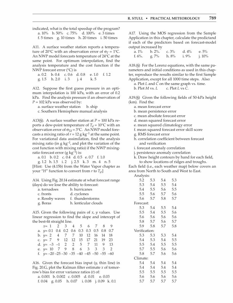
r. Stull • Practical meteorology 789
indicated, what is the total speedup of the program? a. 10% b. 50% c. 75% d. 100% e. 3 times f. 5 times g. 10 times h. 20 times i. 50 times
A11. A surface weather station reports a tempera-ture of 20°C with an observation error of σT = 1°C. An NWP model forecasts temperature of 24°C at the same point. For optimum interpolation, find the analysis temperature and the cost function if the NWP forecast error (°C) is a. 0.2 b. 0.4 c. 0.6 d. 0.8 e. 1.0 f. 1.2 g. 1.5 h. 2.0 i. 3 j. 4 k. 5
A12. Suppose the first guess pressure in an opti-mum interpolation is 100 kPa, with an error of 0.2 kPa. Find the analysis pressure if an observation of P = 102 kPa was observed by: a. surface weather station b. ship c. Southern Hemisphere manual analysis
A13(§). A surface weather station at P = 100 kPa re-ports a dew-point temperature of Td = 10°C with an observation error of σTd = 3°C. An NWP model fore-casts a mixing ratio of r = 12 g kg–1 at the same point. For variational data assimilation, find the analysis mixing ratio (in g kg–1, and plot the variation of the cost function with mixing ratio) if the NWP mixing-ratio forecast error (g kg–1) is: a. 0.1 b. 0.2 c. 0.4 d. 0.5 e. 0.7 f. 1.0 g. 1.2 h. 1.5 i. 2 j. 2.5 k. 3 m. 4 n. 5[Hint: Use (4.15b) from the Water Vapor chapter as your “H” function to convert from r to Td.]
A14. Using Fig. 20.14 estimate at what forecast range (days) do we lose the ability to forecast: a. tornadoes b. hurricanes c. fronts d. cyclones e. Rossby waves f. thunderstorms g. Boras h. lenticular clouds
A15. Given the following pairs of x, y values. Use linear regression to find the slope and intercept of the best-fit straight line. x= 1 2 3 4 5 6 7 8 9 a. y= 0.1 0.4 0.2 0.6 0.3 0.3 0.5 0.8 0.7 b. y= 2 4 7 7 10 12 16 14 18 c. y= 7 9 12 12 15 17 21 19 23 d. y= –3 –1 2 2 5 7 11 9 13 e. y= 10 7 9 8 6 3 3 3 2 f. y= –20 –25 –30 –35 –40 –45 –50 –55 –60
A16. Given the forecast bias input (y, thin line) in Fig. 20.G, plot the Kalman filter estimate x of tomor-row’s bias for error variance ratios (r) of: a. 0.001 b. 0.002 c. 0.005 d. 0.01 e. 0.03 f. 0.04 g. 0.05 h. 0.07 i. 0.08 j. 0.09 k. 0.1
A17. Using the MOS regression from the Sample Application in this chapter, calculate the predictand if each of the predictors based on forecast-model output increased by a. 1% b. 2%. c. 3% d. 4% e. 5% f. 6%. g. 7% h. 8% i. 9% j. 10%
A18.(§) For the Lorenz equations, with the same pa-rameters and initial conditions as used in this chap-ter, reproduce the results similar to the first Sample Application, except for all 1000 time steps. Also: a. Plot L and C on the same graph vs. time. b. Plot M vs. L c. Plot L vs C.
A19.(§) Given the following fields of 50-kPa height (km). Find the: a. mean forecast error b. mean persistence error c. mean absolute forecast error d. mean squared forecast error e. mean squared climatology error f. mean squared forecast error skill score g. RMS forecast error h. correlation coefficient between forecast and verification i. forecast anomaly correlation j. persistence anomaly correlation k. Draw height contours by hand for each field, to show locations of ridges and troughs.Each field (i.e., each weather map) below covers an area from North to South and West to East. Analysis: 5.2 5.3 5.4 5.3 5.3 5.4 5.5 5.4 5.4 5.5 5.6 5.5 5.5 5.6 5.7 5.6 5.6 5.7 5.8 5.7 Forecast: 5.3 5.4 5.5 5.4 5.5 5.4 5.5 5.6 5.6 5.6 5.6 5.6 5.8 5.7 5.6 5.7 5.9 5.8 5.7 5.8 Verification: 5.3 5.3 5.3 5.4 5.4 5.3 5.4 5.5 5.5 5.4 5.5 5.5 5.7 5.5 5.6 5.6 5.8 5.7 5.6 5.6 Climate: 5.4 5.4 5.4 5.4 5.4 5.4 5.4 5.4 5.5 5.5 5.5 5.5 5.6 5.6 5.6 5.6 5.7 5.7 5.7 5.7
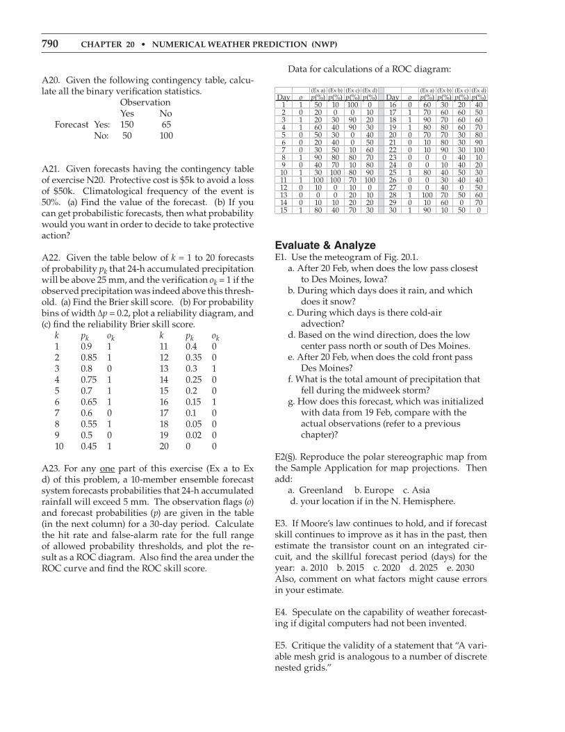
790 chaPter 20 • Numerical Weather PredictioN (NWP)
Data for calculations of a ROC diagram:
(Ex a) (Ex b) (Ex c) (Ex d) (Ex a) (Ex b) (Ex c) (Ex d)Day o p(%) p(%) p(%) p(%) Day o p(%) p(%) p(%) p(%)
1 1 50 10 100 0 16 0 60 30 20 402 0 20 0 0 10 17 1 70 60 60 503 1 20 30 90 20 18 1 90 70 60 604 1 60 40 90 30 19 1 80 80 60 705 0 50 30 0 40 20 0 70 70 30 806 0 20 40 0 50 21 0 10 80 30 907 0 30 50 10 60 22 0 10 90 30 1008 1 90 80 80 70 23 0 0 0 40 109 0 40 70 10 80 24 0 0 10 40 2010 1 30 100 80 90 25 1 80 40 50 3011 1 100 100 70 100 26 0 0 30 40 4012 0 10 0 10 0 27 0 0 40 0 5013 0 0 0 20 10 28 1 100 70 50 6014 0 10 10 20 20 29 0 10 60 0 7015 1 80 40 70 30 30 1 90 10 50 0
evaluate & analyzeE1. Use the meteogram of Fig. 20.1. a. After 20 Feb, when does the low pass closest to Des Moines, Iowa? b. During which days does it rain, and which does it snow? c. During which days is there cold-air advection? d. Based on the wind direction, does the low center pass north or south of Des Moines. e. After 20 Feb, when does the cold front pass Des Moines? f. What is the total amount of precipitation that fell during the midweek storm? g. How does this forecast, which was initialized with data from 19 Feb, compare with the actual observations (refer to a previous chapter)?
E2(§). Reproduce the polar stereographic map from the Sample Application for map projections. Then add: a. Greenland b. Europe c. Asia d. your location if in the N. Hemisphere.
E3. If Moore’s law continues to hold, and if forecast skill continues to improve as it has in the past, then estimate the transistor count on an integrated cir-cuit, and the skillful forecast period (days) for the year: a. 2010 b. 2015 c. 2020 d. 2025 e. 2030Also, comment on what factors might cause errors in your estimate.
E4. Speculate on the capability of weather forecast-ing if digital computers had not been invented.
E5. Critique the validity of a statement that “A vari-able mesh grid is analogous to a number of discrete nested grids.”
A20. Given the following contingency table, calcu-late all the binary verification statistics. Observation Yes No Forecast Yes: 150 65 No: 50 100
A21. Given forecasts having the contingency table of exercise N20. Protective cost is $5k to avoid a loss of $50k. Climatological frequency of the event is 50%. (a) Find the value of the forecast. (b) If you can get probabilistic forecasts, then what probability would you want in order to decide to take protective action?
A22. Given the table below of k = 1 to 20 forecasts of probability pk that 24-h accumulated precipitation will be above 25 mm, and the verification ok = 1 if the observed precipitation was indeed above this thresh-old. (a) Find the Brier skill score. (b) For probability bins of width ∆p = 0.2, plot a reliability diagram, and (c) find the reliability Brier skill score. k pk ok k pk ok 1 0.9 1 11 0.4 0 2 0.85 1 12 0.35 0 3 0.8 0 13 0.3 1 4 0.75 1 14 0.25 0 5 0.7 1 15 0.2 0 6 0.65 1 16 0.15 1 7 0.6 0 17 0.1 0 8 0.55 1 18 0.05 0 9 0.5 0 19 0.02 0 10 0.45 1 20 0 0
A23. For any one part of this exercise (Ex a to Ex d) of this problem, a 10-member ensemble forecast system forecasts probabilities that 24-h accumulated rainfall will exceed 5 mm. The observation flags (o) and forecast probabilities (p) are given in the table (in the next column) for a 30-day period. Calculate the hit rate and false-alarm rate for the full range of allowed probability thresholds, and plot the re-sult as a ROC diagram. Also find the area under the ROC curve and find the ROC skill score.

r. Stull • Practical meteorology 791
E6. What procedure (i.e., what equations and how they are manipulated) would you use to create the 4th-order centered difference of eq. (20.BA6).
E7. If NWP Corollaries 1 and 2 did not exist, de-scribe tricks that you could use to increase the speed of numerical weather forecasts.
E8. Write a finite-difference equation similar to eq. (20.13) for the shaded grid cell of Fig. 20.9, but for: a. vertical advection b. advection in the y-direction
E9. Draw the stencil of grid points used for com-puting horizontal advection, but for the ___ grid for 2nd-order spatial differencing. a. A b. B c. D
E10. If the atmosphere is balanced, and if observa-tions of the atmosphere are perfectly accurate, why would numerical models of the atmosphere start out imbalanced?
E11. For the case study forecast of Figs. 20.15, first photocopy the figures. Then, on each map a. Draw the likely location for fronts. b. Indicate the locations of low centers c. Comment on the forecast accuracy for fronts, cyclones, and the large-scale flow for this case.
E12. Suppose you are making weather forecasts for Pittsburgh, Pennsylvania, which is close to the in-tersection of the 40°N parallel and 80°W meridian, shown by the intersection of latitude and longitude lines in Figs. 20.15 just south of Lake Erie. During the 7.5 days prior to 00 UTC 24 Feb 94, your tempera-ture forecasts for 00 UTC 24 Feb would likely change as you received newer updated forecast maps. What is your temperature forecast for 00 UTC 24 Feb, if you made it ___ days in advance from the EC-MWF forecast charts of Fig. 20.15? a. 7.5 b. 5.5 c. 3.5 d. 1.5 e. and which forecast was closest to the actual verifying analysis?
E13.(§) Suppose the Lorenz equations were modi-fied by assuming that C = L. For the second two Lorenz equations, replace every C with L, and recal-culate for the first 1000 time steps. a. Plot L and M vs. time on the same graph. b. Plot M vs. L.Note that the solution converges to a steady-state so-lution. On the graph of M vs. L, this is called a fixed point. This fixed point is an attractor, but not a strange attractor.
c. Describe what type of physical circulation is associated with this solution.
E14. Experiment with the Lorenz equations on a spreadsheet. Over what range of values of the pa-rameters σ, b, and r, do the solutions still exhibit cha-otic solutions similar to that shown in Fig. 20.18?
E15. A pendulum swings with a regular oscilla-tion. a. Plot the position of the pendulum vs. time. b. Plot the velocity of the pendulum vs. time. c. Plot the position vs. velocity. This is a called a phase diagram according to chaos theory. How does it differ from the phase diagram (i.e., the but-terfly) of the Lorenz strange attractor?
E16. Use the ensemble forecast for Des Moines in Fig. 20.19. a. What 85-kPa temperature forecast, and with what reliability, would you make for forecast day: 1, 3, 5, 7, and 9 ? b. Which temperature ranges would you be confident to forecast would NOT occur, for day: 1, 3, 5, 7, and 9 ? c. In spite of the forecast uncertainty, are you confident about the general trends in temperature? d. Could you confidently forecast when rain is most likely? If so, how much rain would you predict?
E17. Fit an exponential curve to the persistence data of Fig. 20.22. What is the e-folding time?
E18. In what order are weather maps presented in the weather briefing given by your favorite local TV meteorologist? What are the advantages and dis-advantages of this approach compared to the order suggested in this chapter?
SynthesizeS1. Learn what an analog computer is, and how it differs from a digital computer. If automated weath-er forecasts were made with analog rather than digi-tal computers, how would forecasts be different, if at all?
S2. a. Suppose that there were no weather observa-tions in the western half of N. America. How would the forecast quality over Washington, DC, and Ot-tawa, Canada, be different, if at all? Given that na-tional legislators live in those cities, speculate on the changes that they would require of the national

792 chaPter 20 • Numerical Weather PredictioN (NWP)
weather services in the USA and Canada in order to improve the forecasts. b. Extending the discussion from part (a), suppose that weather observations are back to normal in N. America, but the seats of government were moved to Seattle and Vancouver. Given what you know about the Pacific data void, speculate on the changes that they would require of the national weather services in the USA and Canada in order to improve the fore-casts.
S3. How many grid points are needed to forecast over the whole world with roughly 1-m grid spac-ing? When do you anticipate computer power will have the capability to do such a forecast? What, if any, are the advantages to such a forecast?
S4. Design a grid arrangement different from that in Fig. 20.9, but which is more efficient (i.e., involves fewer calculations) or utilizes a smaller stencil.
S5. a. Suppose one person developed and ran a NWP model that gave daily forecasts with twice the skill as those produced by any other NWP model run operationally around the world. What power and wealth could that person accumulate, and how would they do it? What would be the consequences, and who would suffer? b. Same question as part (a), but for one country rather than one person.
S6. Look up the Runge-Kutta finite-difference meth-od in a book or internet site on numerical methods. Find equations for a Runge-Kutta method that is higher order than fourth-order. Can you implement this method on a computer spreadsheet? Try it.
S7. Suppose that there was not a CFL numerical sta-bility criterion that restricted the time step that can be used for NWP. How would NWP be different, if at all? Even without a numerical stability criterion, would there be any other restrictions on the time step? If so, discuss.
S8. Speculate on the ability of national forecast cen-ters to make timely weather forecasts if a computer hacker destroyed the internet and other world-wide data networks.
S9. If greater spread of ensemble members in an ensemble forecast means greater uncertainty, then is greater spread desirable or undesirable in an en-semble forecast?
S10. Which would likely give more-accurate fore-casts: a categorical model with very fine grid spac-ing, or an average of ensemble runs where each en-semble member has coarse grid spacing? Why?
S11. Same as the previous question, but specifically for over steep mountainous terrain. Discuss.
S12. Finite-difference equations are approximations to the full, differential equations that describe the real atmosphere. However, such finite-difference equations can also be thought of as exact represen-tations of a numerical atmosphere that behaves ac-cording to different physics. How is this numeri-cal atmosphere different from the real atmosphere? How would physical laws differ for this numerical atmosphere, if at all? When the NWP model runs for a long time, if it approaches steady state, is this state equal to the real climate or to the “model” cli-mate?
S13. Suppose that electricity did not exist. How would you make numerical weather forecasts? Also, how would you disseminate the results to custom-ers? S14. How good must a numerical forecast be, to be good enough? Should the quality and value of a weather forecast be determined by meteorologists, computer scientists, or end users? Discuss.
S15. Lorenz suggested that there is a limit to pre-dictability. Is that a “hard” limit, or might it be pos-sible to make skillful forecasts beyond that limit? Discuss.
S16. Comment on the interconnectivity of the atmo-sphere, as expressed by NWP corollary 1.


![Data Assimilation for Numerical Weather Prediction - [NWP ......Data Assimilation for Numerical Weather Prediction [NWP] Project Ahmed Attia Statistical and Applied Mathematical Science](https://static.fdocuments.in/doc/165x107/6039cba9995b992a170c4a78/data-assimilation-for-numerical-weather-prediction-nwp-data-assimilation.jpg)