Opening the Black Box:Low-dimensional dynamics in high-dimensional

recurrent neural networks

David Sussillo∗

sussillo@stanford.eduDepartment of Electrical Engineering

Neurosciences ProgramStanford University

Stanford, California 94305-9505

and

Omri Barak∗

ob2194@columbia.eduDepartment of Neuroscience

Columbia University College of Physicians and SurgeonsNew York NY 10032-2695

present address:Rappaport Faculty of Medicine,

Technion Israeli Institute of Technology,Haifa, Israel

∗ Equal contribution

Abstract

Recurrent neural networks (RNNs) are useful tools for learning nonlinear rela-tionships between time-varying inputs and outputs with complex temporal depen-dencies. Recently developed algorithms have been successful at training RNNsto perform a wide variety of tasks, but the resulting networks have been treatedas black boxes – their mechanism of operation remains unknown. Here we ex-plore the hypothesis that fixed points, both stable and unstable, and the linearizeddynamics around them, can reveal crucial aspects of how RNNs implement theircomputations. Further, we explore the utility of linearization in areas of phase-space that are not true fixed points, but merely points of very slow movement. Wepresent a simple optimization technique that is applied to trained RNNs to find thefixed points and slow points of their dynamics. Linearization around these slowregions can be used to explore, or reverse-engineer, the behavior of the RNN.We describe the technique, illustrate it on simple examples, and finally showcaseit on three high-dimensional RNN examples: a 3-bit flip-flop device, an input-dependent sine wave generator and a two-point moving average. In all cases, themechanisms of trained networks could be inferred from the sets of fixed and slowpoints and the linearized dynamics around them.

2

1 IntroductionA recurrent neural network (RNN) is a type of artificial neural network with feed-back connections. Because the network has feedback it is ideally suited for prob-lems in the temporal domain such as implementing temporally complex input-output relationships, input-dependent pattern generation, or autonomous patterngeneration. However, training RNNs is widely accepted as a difficult problem(Bengio et al., 1994). Recently, there has been progress in training RNNs toperform desired behaviors (Maass et al., 2002; Jaeger and Haas, 2004; Maasset al., 2007; Sussillo and Abbott, 2009; Martens and Sutskever, 2011). Jaegerand Hass developed a type of RNN called an echostate network, which achievesgood performance by allowing for a random recurrent pool to receive feedbackfrom a set of trained output units (Jaeger and Haas, 2004). Sussillo and Ab-bott (Sussillo and Abbott, 2009) derived a rule to train the weights of such anechostate network operating in the chaotic regime. Further, Martens and Sutskever(Martens and Sutskever, 2011) employed a second-order optimization techniquecalled Hessian-Free optimization to train all the weights in an RNN using back-propagation through time to compute the gradient (Rumelhart et al., 1985). Giventhese recent developments, it is likely that RNNs will enjoy more popularity in thefuture than they have to date.

Because such supervised training algorithms specify the function to performwithout specifying how to perform it, the exact nature of how these trained RNNsimplement their target functions remains an open question. The resulting networksare often viewed as black boxes. This is in contrast to network models that wereexplicitly constructed to implement a specific known mechanism (e.g. see (Wang,2008; Hopfield, 1982)). One way to make progress may be to view an RNN as anonlinear dynamical system (NLDS) and, in this light, there is a rich tradition ofinquiry that can be exploited.

A nonlinear dynamical system is, as the name implies, nonlinear. As such, thequalitative behavior of the system varies greatly between different parts of phasespace and can be very difficult to understand. A common line of attack whenanalyzing NLDSs is therefore to study different regions in phase space separately.The most common anchors to begin such analyses are fixed points. These arepoints in phase space exhibiting zero motion, with the invaluable property thatthe dynamics near a fixed point are approximately linear and thus easy to analyze.Other, faster, points in phase space can also provide insight into the system’s modeof operation, but are harder to systematically locate and analyze.

In this contribution, we show that there are other regions in phase space, which

3

we call slow points, where linearization is valid. Our hypothesis is that under-standing linearized systems around fixed and slow points in the vicinity of typ-ical network trajectories can be insightful regarding computational mechanismsof RNNs. We provide a simple optimization technique for locating such regions.The full analysis would therefore entail finding all candidate points of the RNN,linearizing the dynamics around each one, and finally trying to understand theinteraction between different regions (Strogatz, 1994; Ott, 2002). We illustratethe application of the technique using both fixed points and slow points. Theprinciples are first illustrated with a simple two-dimensional example, followedby high-dimensional trained RNNs performing memory and pattern generationtasks.

2 Fixed pointsAs stated in the introduction, fixed points are common anchors to start analysisof the system. Fixed points are either stable or unstable, meaning that the motionof the system, when started in the vicinity of a given fixed point, either convergestowards or diverges away from that fixed point, respectively. Stable fixed points,also known as attractors, are important because the system will converge to them,or, in the presence of noise, dwell near them. Unstable fixed points come in morevarieties, having one or more unstable modes, up to the case of a completelyunstable fixed point (repeller). A mode is an independent pattern of activity thatarises when the linear system is diagonalized. When attempting to understand theinteraction between different attractors, unstable fixed points with a few unstablemodes are often very useful. For instance, a saddle point with one unstable modecan funnel a large volume of phase space through its many stable modes, and thensend them to two different attractors depending on which direction of the unstablemode is taken.

Finding stable fixed points is often as easy as running the system dynamicsuntil it converges (ignoring limit cycles and strange attractors). Finding repellersis similarly done by running the dynamics backwards. Neither of these methods,however, will find saddles. The technique we introduce allows these saddle pointsto be found, along with both attractors and repellers. As we will demonstrate,saddle points that have mostly stable directions, with only a handful of unstabledirections, appear to be of high significance when studying how RNNs accomplishtheir tasks (a related idea is explored in (Rabinovich et al., 2008)).

4

3 Linear approximationsConsider a system of first-order differential equations

x = F(x), (1)

where x is an N-dimensional state vector and F is a vector function that definesthe update rules (equations of motion) of the system. We wish to find values x∗around which the system is approximately linear. Using a Taylor series expansion,we expand F(x) around a candidate point in phase space, x∗:

F(x∗ + δx) = F(x∗) + F′(x∗)δx +12δxF′′(x∗)δx + . . . (2)

Because we are interested in the linear regime, we want the first derivative termof the right hand side to dominate the other terms. Specifically, we are looking forpoints x∗, and perturbations around them, δx ≡ x − x∗, such that

|F′(x∗)δx| > |F(x∗)| (3)

|F′(x∗)δx| >∣∣∣∣∣12δxF′′(x∗)δx

∣∣∣∣∣ . (4)

From inequality 3 it is evident why fixed points (x∗ such that F(x∗) = 0) are goodcandidates for linearization. Namely, the lower bound for δx is zero, and thusthere is always some region around x∗ where linearization should be valid. Theyare not, however, the only candidates. A slow point, having a non-zero, but small,value of F(x∗) could be sufficient for linearization. In this case, examining thelinear component of the computations of a RNN may still be reasonable becausethe inequalities can still be satisfied for some annulus-like region around the slowpoint.

Allowing |F(x∗)| > 0 means we are defining an affine system, which can bedone anywhere in phase space. However, inequalities 3 and 4 highly limit theset of candidate points we are interested in. So we end up examining true linearsystems at fixed points and affine systems at slow points. The latter are not genericaffine systems since the constant is so small as to be negligible at the time scaleon which the network operates. It is in these two ways that we use the termlinearization.

5

This observation motivated us to look for regions where the norm of the dy-namics, |F(x)|, is either zero or small. To this end, we define an auxiliary scalarfunction

q(x) =12|F(x)|2 . (5)

Intuitively, the function q is related to the speed, or kinetic energy of the sys-tem. Speed is the magnitude of the velocity vector, so q is the squared speeddivided by two, which is also the expression for the kinetic energy of an objectwith unit mass.

There are several advantages to defining q in this manner. First, it is a scalarquantity and thus amenable to optimization algorithms. Second, as q is a sum ofsquares, q(x∗) = 0 if and only if x∗ is a fixed point of F. Third, by minimizing|F(x)|, we can find candidate regions for linearization that are not fixed points, as-suming inequalities 3 and 4 are satisfied, thus expanding the scope of linearizationtechniques.

To understand the conditions when q is at a minimum, consider the gradientand Hessian of q:

∂q∂xi

=

N∑k

∂Fk

∂xixk (6)

∂2q∂xi∂x j

=

N∑k

∂Fk

∂xi

∂Fk

∂x j+

N∑k

xk∂2Fk

∂xi∂x j. (7)

For q to be at a minimum, the gradient (equation 6) has to be equal to the zerovector, and the Hessian (equation 7) has to be positive definite. There are threeways for the gradient to be zero.

1. If xk = 0, for all k, then the system is at a fixed point, and this is a globalminimum of q.

2. If the entire Jacobian matrix, ∂Fi∂x j

(x), is zero at x, and the second term of theHessian is positive definite, then q may be at a local minimum.

3. Finally, q may be at a minimum if x is a zero eigenvector of ∂F∂x . For high-

dimensional systems, this is a much less stringent requirement than the pre-vious one, and thus tends to be most common for local minima in RNNs.

6

In summary, our approach consists of using numerical methods to minimizeq to find fixed points and slow points. Because the systems we study may havemany different regions of interest, the optimization routine is run many times fromdifferent initial conditions (ICs) that can be chosen based on the particular prob-lem at hand. Typically, these ICs are points along RNN system trajectories duringcomputations of interest. In the following sections, we will demonstrate our ap-proach on cases involving fixed points for both low- and high- dimensional sys-tems. Then we will show the advantages of linearizing around regions that are notfixed points.

3.1 Two-dimensional exampleA simple 2D example helps to demonstrate minimization of the auxiliary functionq and evolution of x = F(x). For this section, we define the dynamical systemx = F(x) as follows

x1 = (1 − x21)x2 (8)

x2 = x1/2 − x2. (9)

The system has three fixed points: A saddle at (0, 0) and two attractors at (1, 1/2)and (−1,−1/2). Based on this definition of F, the function q is defined as

q(x) = 12

(x2

2

(1 − x2

1

)2+ (x1/2 − x2)2

). Note that the fixed points of x = F(x) are

the zeros of q.A number of system trajectories defined by evolving the dynamical system

x = F(x) are shown in Figure 1 in thick black lines. The three fixed points of x =

F(x) are shown as large ’x’s. The color map shows the values of q(x), pink codeslarge values and cyan codes small values. This color map helps in visualizing howminimization of q proceeds.

Studying the system trajectories alone might lead us to suspect that a saddlepoint is mediating a choice between two attractors (black ’x’). But the location ofthis hypothetical saddle is unknown. Using trajectories that are close to the saddlebehavior, we can initiate several sample minimizations of q (thick red lines), andsee that indeed two of them lead to the saddle point (green ’x’). For this example,two different minimization trajectories originate from the same trajectory of thedynamical system.

7

x1

x 2

−1 −0.5 0 0.5 1−0.8

−0.6

−0.4

−0.2

0

0.2

0.4

0.6

0.8

−18

−16

−14

−12

−10

−8

−6

−4

−2

0

log10q

Figure 1: A 2D example of the behavior of minimization of q relative to thedefining dynamical system. The trajectories of a simple 2D dynamical system,x = F(x), defined as x1 = (1−x2

1)x2, x2 = x1/2−x2 are shown in thick black lines.Shown with black ’x’ are the two attractors of the dynamical system. A saddlepoint is denoted with a green ’x’. Gradient descent on the auxiliary function q isshown in thick red lines. Minimization of q converges to one of the two attractorsor to the saddle point, depending on the IC. The value of q is shown with a colormap (bar indicates log10 q) and depends on the distance to the fixed points ofx = F(x).

3.2 RNNsNow consider x = F(x) defined as a recurrent neural network,

xi = −xi +

N∑k

Jikrk +

I∑k

Bikuk (10)

ri = h (xi) , (11)

8

where x is the N-dimensional state called the “activations”, r = h(x) are the “fir-ing rates”, defined as the element-wise application of the nonlinear function hto x. The recurrence of the network is defined by the matrix J and the networkreceives the I-dimensional input u through the synaptic weight matrix B. In thecases we study, which are typical of training from random initialization, the matrixelements, Jik, are taken from a normal distribution with zero mean and varianceg2/N, where g is a parameter that scales the network feedback.

After random initialization, the network is trained, typically with a supervisedlearning method. We assume that such an RNN has already been optimized toperform either an input-output task or a pattern generation task. Our goal is toexplore the mechanism by which the RNN performs the task by finding the fixedpoints and slow points of x = F(x) and the behavior of the network dynamicsaround those points.

To employ the technique on the RNN defined by equations 10-11, we defineq as before, q(x) = 1

2 |F(x)|2. The Jacobian of the network, useful for defining thegradient and Hessian of q, is given by

∂Fi

∂x j= −δi j + Ji jr′j, (12)

where δi j is defined to be 1 if i = j, and otherwise 0. Also, r′j is the derivative ofthe nonlinear function h, with respect to its input, x j.

3.3 3-Bit flip-flop exampleWe now turn to a high-dimensional RNN implementing an actual task. We firstdefine the task, then describe the training and show performance of the network.Finally, we use our technique to locate the relevant fixed points of the system anduse them to understand the underlying network mechanism.

Consider the 3-bit flip-flop task shown in Figure 2. A large recurrent networkhas 3 outputs showing the state of 3 independent memory bits. Transient pulsesfrom three corresponding inputs set the state of these bits. For instance, input2 (dark green) is mostly zero, but at random times emits a transient pulse thatis either +1 or -1. When this happens, the corresponding output (output 2, lightgreen) should reflect the sign of the last input pulse, taking and sustaining a valueof either +1 or -1. For example, the first green pulse does not change the memorystate, because the green output is already at +1. The second green pulse, however,does. Also, the blue and red pulses should be ignored by the green output. An

9

+1

-1

-1

-1

+1

+1

Time

Figure 2: Example inputs and outputs for the 3-bit flip-flop task. Left panel.Sample input and output to the 3-bit flip-flop network. The three inputs and out-puts are shown in pairs (dark red / red, dark green / green and dark blue / blue,respectively). Brief input pulses come in with random timing. For a given input/ output pair, the output should transition to +1 or stay at +1 for an input pulseof +1. The output should transition to -1 or stay at -1 if the corresponding in-put pulse is -1. Finally, all three outputs should ignore their non-matching inputpulses. Right panel. Network with echostate architecture used to learn the 3-bitflip-flop task. Trained weights are shown in red.

RNN that performs this task for 3 input/output pairs must then represent 23 = 8memories and so is a 3-bit flip-flop device, while ignoring the cross-talk betweendiffering input / output pairs.

We trained a randomly connected network (N = 1000) to perform the 3-bitflip-flop task using the FORCE learning algorithm(Sussillo and Abbott, 2009)(see Methods). We then performed the linearization analysis, using the trajecto-ries of the system during operation as ICs. Specifically, we spanned all possibletransitions between the memory states using the inputs to the network, and thenrandomly selected 600 network states out of these trajectories to serve as ICs forthe q optimization. The algorithm resulted in 26 distinct fixed points, on whichwe performed a linear stability analysis. Specifically, we computed the Jacobianmatrix, equation 12, around each fixed point and performed an eigenvector de-composition on these matrices.

The resulting stable fixed points and saddle points are shown in Figure 3, leftpanel. To display the results of these analyses, the network state x(t) is plotted

10

in the basis of the first three principal components of the network activations (thetransient pulses reside in other dimensions, one is shown in the right panel ofFigure 3). In black ’x’ are the fixed points corresponding to each of the 8 mem-ory states. These fixed points are attractors and the perturbative linear dynamicsaround each fixed point are stable. Shown in blue are the 24 neural trajectories(activation variable x) showing the effect of an input pulse that flips the 3-bit flip-flop system by one bit. The green ’x’ are saddles, fixed points with 1 unstabledimension and N-1 stable dimensions. Shown in thin red lines are network trajec-tories started just off the saddle on the dimension of instability. As we will show,the saddles are utilized by the system to mediate the transition from one memorystate to another (shown in detail on the right panel). Finally, shown in magenta ’x’are 2 fixed points with 4 unstable dimensions each (thick red lines). Again, samplenetwork trajectories were plotted with the ICs located just off each fixed point onthe 4 dimensions of instability. The unstable trajectories appear to connect threememory states, with no obvious utility.

To verify whether indeed the saddle points are utilized by the system to switchfrom one memory to another we focus on a single transition, specifically frommemory (-1,-1,-1) to memory( 1, -1, -1). We chose a visualization space thatallows both the effects of input perturbation and memory transitions in state space(PC3 and the relevant input vector) to be seen. We varied the amplitude of therelevant input pulse in small increments from 0 to 1 (Figure 3, right panel). In blueis shown the normal system trajectory (pulse amplitude 1) during the transition forboth the input driven phase and the relaxation phase. In cyan are shown the resultsof an input perturbation experiment using intermediate pulse sizes. Intermediateamplitude values result in network trajectories that are ever closer to the saddlepoint, illustrating its mechanistic role in this particular memory transition.

It is important to note that this network was not designed to have 8 attractorsand saddle points between them. In fact, as Figure 3 shows, there can be morethan one saddle point between two attractors. This is in contrast to networksdesigned to store 8 patterns in memory (Hopfield and Tank, 1986) where no such”redundant” saddle points appear.

3.4 Sine wave generator exampleNext, we demonstrate that our analysis method is effective in problems involvingpattern generation. Because pattern generation may involve system trajectoriesthat are very far from any particular fixed point, it is not obvious a priori thatfinding fixed points is helpful. For our pattern generation example, we trained a

11

PC1

InputDriven

InputPC2

PC3PC3

Relaxation

(1,-1,-1)

(-1,-1,-1)

Figure 3: Low-dimensional phase space representation of 3-bit flip-flop task.Left Panel - The 8 memory states are shown as black ’x’. In blue are shown all24 1-bit transitions between the 8 memory states of the 3-bit flip-flop. The saddlefixed points with 1 unstable dimension are shown with green ’x’. A thick red linedenotes the dimension of instability of these saddles points. In thin red are thenetwork trajectories started just off the unstable dimensions of the saddle points.These are heteroclinic orbits between the saddles that decide the boundaries andthe attractor fixed points that represent the memories. Finally, with magenta ’x’are shown other fixed points, all with 4 unstable dimensions. Thick red lines showthese dimensions of instability and thin red lines show network trajectories startedjust off the fixed points in these unstable dimensions. Right Panel - Demonstrationthat a saddle point mediates the transitions between attractors. The input for atransition (circled region in left panel) was varied from 0 to 1 and the networkdynamics are shown (blue for normal input pulse and cyan for the rest). As theinput pulse increased in value, the network came ever closer to the saddle, andthen finally transitioned to the new attractor state.

12

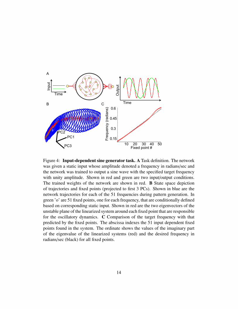
network (N = 200) that received a single input, which specified 1 out of 51 fre-quency values in radians per unit time. The output of the network was defined tobe a sine wave with the specified target frequency and unity amplitude. The targetfrequency was specified by a static input (see Methods and Figure 4A). Again, weperformed the analysis, starting from ICs in the 51 different oscillation trajecto-ries. We took care to include the correct static input value for the optimizationof q (see Methods). This means the fixed points found were conditionally depen-dent on their respective static input value and did not exist otherwise. With thisanalysis we found a fixed point for all oscillations centered in the middle of thetrajectory1.

For all 51 fixed points, a linear stability analysis revealed that the linearizedsystem had only two unstable dimensions and N-2 stable dimensions. A statespace portrait showing the results of the fixed point and linear stability analyses isshown in Figure 4B. The network state (activation variable x) is plotted in the basisof the first three principal components of the network activations. Shown in blueare the neural trajectories for all 51 oscillations. The green ’o’ show each of the 51fixed points, with the unstable modes denoted by red lines. As mentioned above,the actual dynamics are far from the fixed points, and thus not necessarily influ-enced by them. To show that the linear analysis can provide a good descriptionof the dynamics, we compared the absolute value of the imaginary components ofone of the two unstable dimensions (they come in complex conjugate pairs) to thedesired frequency in radians specified in the target trajectories (Figure 4C). Thereis very good agreement between the target frequency and the absolute value ofthe imaginary part of the unstable mode of the linearized systems (proximity ofred circles to the black ’x’s), indicating that the oscillations defined by the lineardynamics around each fixed point explained the behavior of the RNN for all targetfrequencies. We verified that the validity of the linear approximation stems fromthe inequalities 3 and 4, by computing the norms of the linear and quadratic termsof the Taylor expansion. Indeed, for all 51 trajectories, the norm of the linear termwas at least twice that of the quadratic term (not shown).

1For the four slowest oscillations we found exactly two fixed points, one centered in the middleof the oscillation with the other outside the trajectory. All other oscillations had exactly one fixedpoint. Based on the results of our stability analysis, for these four oscillations with two fixed points,we focused on the fixed point centered in the middle of the oscillation, which was consistent withhow the oscillations with one fixed point worked.

13

10 20 30 40 50

0.15

0.3

0.45

0.6

A

PC1PC2

PC3

Time

Inpu

t

Fre

quen

cy (

radi

ans)

Fixed point #

B C Time

Out

put

Figure 4: Input-dependent sine generator task. A Task definition. The networkwas given a static input whose amplitude denoted a frequency in radians/sec andthe network was trained to output a sine wave with the specified target frequencywith unity amplitude. Shown in red and green are two input/output conditions.The trained weights of the network are shown in red. B State space depictionof trajectories and fixed points (projected to first 3 PCs). Shown in blue are thenetwork trajectories for each of the 51 frequencies during pattern generation. Ingreen ’o’ are 51 fixed points, one for each frequency, that are conditionally definedbased on corresponding static input. Shown in red are the two eigenvectors of theunstable plane of the linearized system around each fixed point that are responsiblefor the oscillatory dynamics. C Comparison of the target frequency with thatpredicted by the fixed points. The abscissa indexes the 51 input dependent fixedpoints found in the system. The ordinate shows the values of the imaginary partof the eigenvalue of the linearized systems (red) and the desired frequency inradians/sec (black) for all fixed points.

14

4 Beyond fixed pointsWhile fixed points are obvious candidates for linearization, they are not the onlypoints in phase space where linearization makes sense. Minimizing q can lead toregions with a dominating linear term in their Taylor expansion, even if the zeroorder term is non-zero. We first show a 2D example where considering a localminimum of q can provide insight into the system dynamics. Then, we analyze ahigh-dimensional RNN performing a 2-point moving average of randomly timedinput pulses, and demonstrate that points in phase space with small, nonzero val-ues of q can be instructive in reverse engineering the RNN.

4.1 Local minima of q

Consider the 2D dynamical system defined by

x1 = x2 −(x2

1 + 1/4 + a)

(13)

x2 = x1 − x2. (14)

This system has two nullclines that intersect for a ≤ 0. In this case, q will havetwo minima coinciding with the fixed points (Figure 5, left panel). At a = 0the system undergoes a saddle-node bifurcation, and if a is slightly larger than0, there is no longer any fixed point. The function q, however, still has a localminimum exactly between the two nullclines at xg = (1/2, 1/2 + a/2). This canbe expected, because q measures the speed of the dynamics, and this ghost of afixed point is a local minimum of speed. The system trajectories shown in Figure5, right panel, indicate that this point represents a potentially interesting area ofthe dynamics, as it funnels the trajectories into one common pathway, and thedynamics are considerably slower near it (not shown in the figure).

While finding the location of such a ghost can be useful, we will go beyond itand consider the linear expansion of the dynamics around this point:

(x1

x2

)= F

(xg +

(dx1

dx2

))=

(−1 11 −1

) (dx1

dx2

)−

a2

(11

)(15)

As expected from our discussion of conditions for minima of q, the Jacobianhas one zero eigenvalue with eigenvector (1, 1). The second eigenvalue is −

√2,

with an orthogonal eigenvector (1,−1). The full behavior near xg is therefore

15

−4 −2 0 2 4−4

−2

0

2

4

x1

x 2

−4 −2 0 2 4−4

−2

0

2

4

x1x 2

Figure 5: Ghosts and local minima of q. Left Panel - Dynamics of the systemdescribed by equations 13 and 14 with a = −0.3. There are two fixed points – asaddle and a node (red points), both located at the intersection of the two nullclines(green lines), and are global minima of q. Right Panel - The same system witha = 0.3. There are no fixed points, but the local minimum of q (red point) denotesa ghost of a fixed point, and clearly influences the dynamics. The linear expansionaround this ghost reveals a strongly attracting eigenvector (pink inward arrows),corresponding to the dynamics, and a zero eigenvector (pink lines), along whichthe dynamics slowly flows as the system is not at a true fixed point.

attraction along one axis and a slow drift along the other, the latter arising fromthe fact that xg is not a true fixed point (magenta lines in the figure inset). Thoughlacking any fixed point, the dynamics of this system can still be understood usinglinearization around a candidate point, with the additional understanding that thedrift will affect the system on a very slow time scale.

In general, when linearizing around a slow point, xs, the local linear systemtakes the form

δx = F′(xs) δx + F(xs), (16)

where the zero order contribution, F(xs), can be viewed as a constant input to thesystem. While equation 16 makes sense for any point in phase space, it is theslowness of the point as defined by inequalities 3 and 4 that makes the equationuseful. In practice, we’ve found that the constant term, F(xs), is negligible, but weinclude it for correctness.

16

10 20 30 40 50 60 70−1

−0.5

0

0.5

1

Time (s)

Inpu

t / O

utpu

t / T

arge

t Val

ues

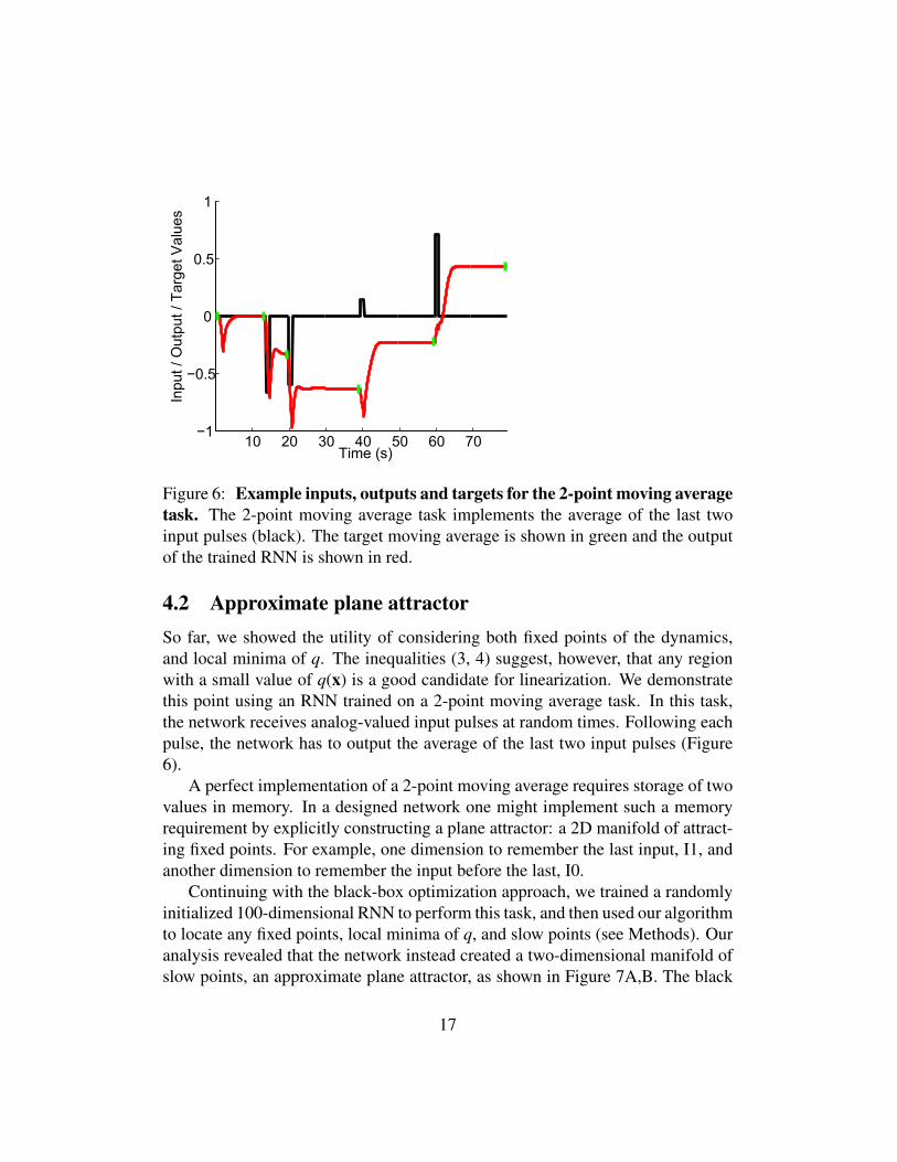
Figure 6: Example inputs, outputs and targets for the 2-point moving averagetask. The 2-point moving average task implements the average of the last twoinput pulses (black). The target moving average is shown in green and the outputof the trained RNN is shown in red.

4.2 Approximate plane attractorSo far, we showed the utility of considering both fixed points of the dynamics,and local minima of q. The inequalities (3, 4) suggest, however, that any regionwith a small value of q(x) is a good candidate for linearization. We demonstratethis point using an RNN trained on a 2-point moving average task. In this task,the network receives analog-valued input pulses at random times. Following eachpulse, the network has to output the average of the last two input pulses (Figure6).

A perfect implementation of a 2-point moving average requires storage of twovalues in memory. In a designed network one might implement such a memoryrequirement by explicitly constructing a plane attractor: a 2D manifold of attract-ing fixed points. For example, one dimension to remember the last input, I1, andanother dimension to remember the input before the last, I0.

Continuing with the black-box optimization approach, we trained a randomlyinitialized 100-dimensional RNN to perform this task, and then used our algorithmto locate any fixed points, local minima of q, and slow points (see Methods). Ouranalysis revealed that the network instead created a two-dimensional manifold ofslow points, an approximate plane attractor, as shown in Figure 7A,B. The black

17

A B

−2−1012−202

−0.5

0

0.5

−1.5−1

−0.50

0.51

−1

−0.5

0

0.5

1

0

0.5

1

1.5

PC1

PC1

PC2

PC3 PC3

PC2

Figure 7: 2D approximate plane attractor in 2-point moving average task.The 2-point moving average task requires two variables to complete the task. TheRNN holds those two variables in an approximate plane attractor. A The slowpoints (q ≤ 1e-4) form a 2D manifold. The black ’+’ show the slow points of thenetwork. All slow points have two modes with approximately zero eigenvalues.B Dynamical picture of 2D manifold of slow points. There are two fixed points(grey ’x’), one with two stable directions tangent to the manifold and another withone stable and one unstable dimension tangent to the manifold. The network wassimulated for 1000s from slow points on the manifold (q ≤ 1e-7) as the ICs. Theseslow trajectories are shown with blue lines ending in arrows. To compare with thefast time scales of normal network operation, we show the network computing amoving average that includes a new input. This network trajectory lasted for about30s (orange). Each ∆t of the one second input is shown with orange squares.

’+’ in panel A show all points with values of q smaller than 1e-4 in the space of thefirst 3 principal components. The linearized dynamics around all slow points hadtwo modes with approximately zero eigenvalues and N-2 fast decaying modes.

In addition to the many slow points, the optimization found two fixed points.These two fixed points organize the extremely slow dynamics on the approximateplane attractor. Shown in Figure 7B is the dynamical structure on the 2D mani-fold. Each slow point was used as an IC to the network and the network run for1000s (blue trajectories with arrows). These trajectories demonstrate the precisedynamics at slow time scales that become the approximately fixed dynamics atthe timescale of normal network operation. To demonstrate the fast decaying dy-namics to the manifold, the network was run normally with a single trial, whichtook around 30s (orange trajectory).

18

To test the utility of linearizing the RNN around the slow points, we attemptedto replace the full nonlinear system with a succession of linear systems defined bythe slow points (Figure 8). Specifically, we defined a linear time-varying dynami-cal system (LTVDS, see Methods), in which the dynamics at each time point werethe linear dynamics induced by the closest slow point. We then compared the statetransition induced by a single input pulse as implemented by both the RNN andthe LTVDS across many random inputs and ICs (Figure 8A,B show examples).Note that whenever a new input pulse comes in, the network dynamics must im-plement two transitions. The I1 value must shift to the I0 value and the latestinput pulse value must shift to the I1 value. Our test of the LTVDS approximationthus measured the mean squared error between the RNN and the LTVDS for theshifted values I1 to I0 and input to I1 (Figure 8, panels C and D, respectively).The errors were 0.074, and 0.0067, for I1→I0 and input→I1.

Finally, we demonstrate that our method is not dependent on a finely tunedRNN. We structurally perturbed the RNN that implemented the 2-point mov-ing average by adding to the recurrent matrix random Gaussian noise with zeromean and standard deviation, η (see Methods). The dependency of the outputerror on the size of the structural perturbation is shown in Figure 9A. An exam-ple perturbed RNN with network inputs and output is shown in Figure 9B, withη = 0.006. Unsurprisingly, the main problem is a drift in the output value, indicat-ing that the quality of the approximate plane attractor has been heavily degraded.We applied our technique to the structurally perturbed network to study the effectsof the perturbation. Figures 9C,D show that the same approximate plane attrac-tor dynamical structure is still in place, though much degraded. The slow pointmanifold is still in the same approximate place, although the q values of all slowpoints increased. In addition, there is a fixed point detached from the manifold.Nevertheless, the network is able to perform with mean squared error less than0.01, on average.

5 DiscussionRecurrent neural networks, when used in conjunction with recently developedtraining algorithms, are powerful computational tools. The downside of thesetraining algorithms is that the resulting networks are often extremely complex anso their underlying mechanism remains unknown. Here we used methods fromnonlinear dynamical system theory to pry open the black box. Specifically, weshowed that finding fixed points and slow points (points where inequalities (3, 4)

19

−1 0 1

−1

0

1

Input pulse value

I1

−2 −1 0 1 2

−2

0

2

I0

−101−3

0

0

1

2

3

I0I1

0 20 40 60 80-1

-0.6

-0.2

0.2

0.6

1

Time (s)

Inpu

t/Out

put/T

arge

t val

ues

PC1

PC

3

A

PC2

I1

B

C D

Figure 8: Comparison of the transition dynamics between the RNN and thelinear time-varying approximation. A Four separate trials of the RNN (redlines) and the LTVDS approximation (dotted red lines). B The same trials plottedin the space of the first three PCs of the network activity. The orange squares showthe ICs, based on the input pulse, given to both RNN and LTVDS. The RNN tra-jectories are orange, the LTVDS are dotted orange. Black dots are the 2000 slowpoints used in simulating the LTVDS. C, D In implementing the 2-point movingaverage, whenever a new input pulse comes in, the RNN must successfully shiftthe value of the last input (I1) to the value of the input before last (I0), panel C,and move the input pulse value to the the value of the last input (I1), panel D. Inblue are the transitions implemented by the RNN. In red are the transitions imple-mented by the LTVDS using the same ICs. The mean squared error between theLTVDS and the RNN for both transitions was 0.074 and 0.0067, respectively.

20

20 40 60 80 100−1

0

1

Time (s)

Inpu

t/Out

put/T

arge

t Val

ues

Mea

n sq

uare

d er

ror

10-6

-4

-2

−11

3 −11

3−1

Perturbation Level

PC

3

5 10 15 20

−11

3 −11

3−1

0

Perturbed Network

PC

310

10

10-6 -4 -2

10 10

PC2PC1PC2PC1

Original Network-log10q =

A

C

B

D

Figure 9: Structural perturbations. A To study the ability of our method to findmeaningful structure in a perturbed network, Gaussian noise was added to therecurrent matrix of the RNN with 0 mean and standard deviation η. The red ’x’marks the η = 0.006 noise level used in further studies. We show a plot of meansquared error of the RNN output as a function of the noise level, η. B Exampleof perturbed network with η = 0.006. Same color scheme as Figure 6. C A viewof the 2D slow point manifold showing the variability in values of q along themanifold for the original network. D Similar to (C) for the perturbed network.Note that all q values are higher in this case.

21

are satisfied) near relevant network trajectories and studying the linear approxi-mations around those points is useful. To this end, we outlined an optimizationapproach to finding slow points, including fixed points, based on the auxiliaryfunction q. Depending on usage, minimization of this function finds global andlocal minima, and also regions in phase space with an arbitrarily specified slow-ness.

We demonstrated how true fixed points were integrally involved in how anRNN solves the 3-bit flip-flop task, creating both the memory states and the saddlepoints to transition between them. We also analyzed an RNN trained to generatean input-dependent sine wave, showing that input-dependent fixed points were re-sponsible for the relevant network oscillations, despite those oscillations occuringfar from the fixed points. In both cases we found that saddle points with primar-ily stable dimensions and only a couple of unstable dimensions were responsiblefor much of the interesting dynamics. In the case of the 3-bit flip-flop, saddlesimplemented the transition from one memory state to another. For the sine wavegenerator the oscillations could be explained by the slightly unstable oscillatorylinear dynamics around each input-dependent saddle point.

Finally, we showed how global minima, local minima and regions of slowspeed were used to create an approximate plane attractor, necessary to implementa 2-point moving average of randomly timed input pulses. The approximate planeattractor was implemented using mainly slow points along a 2D manifold.

There are several reasons why studying slow points, and not only fixed points,is important. First, a trained network does not have to be perfect – few realistictasks require infinite memory or precision, so it could be that forming a slow pointis a completely adequate solution for the defined timescales a given input/outputrelationship. Second, in the presence of noise, the behavior of a fixed point anda very slow point might be indistinguishable. Third, funneling network dynamicscan be achieved by a slow point, and not a fixed point (Figure 5). Fourth, neithertrained networks nor biological ones can be expected to be perfect. Studying theslow points of the perturbed plane attractor showed that our technique is sensitiveenough to detect dynamical structure in a highly perturbed or highly approximatestructure.

The 3-bit flip-flop example was trained using the FORCE learning rule (Sus-sillo and Abbott, 2009), which affected the network dynamics by modifying thethree output vectors. The input-dependent sine wave generator and 2-point mov-ing average were trained using the Hessian-Free optimization technique for RNNs(Martens and Sutskever, 2011) and all the synaptic strengths and biases were mod-ified. Despite the profound differences in these two training approaches, our fixed

22

point method was able to make sense of the network dynamics in both cases.Even though the RNNs we trained were high-dimensional, the tasks we trained

them on were intentionally simple. It remains to be seen whether our techniquecan be helpful in dissecting higher-dimensional problems, and almost certainlydepends on the task at hand as the input and task definition explicitly influencethe dimensionality of the network state.

Our technique, and the dynamical concepts explored using it, may also provideinsight on the observed experimental findings of low-dimensional dynamics in in-vivo neuroscience experiments, (Romo et al., 1999; Stopfer et al., 2003; Joneset al., 2007; Ahrens et al., 2012). For example, we found that a saddle point fun-nels large volumes of phase space into two directions and so may be a dynamicalfeature used in neural circuits that inherently reduces the dimension of the neuralactivity. Since the networks we studied were trained as opposed to designed, andtherefore initially their implementation was unknown, our method and results arecompatible with studies attempting to understand biological neural circuits, forexample, (Huerta and Rabinovich, 2004; Machens et al., 2005; Rabinovich et al.,2008; Liu and Buonomano, 2009; Ponzi and Wickens, 2010).

There are several possible interesting extensions to this technique. While thesystem and examples we studied were continuous in nature, the application ofour technique to discrete RNNs presents no difficulties. Another extension is toapply the fixed point and slow point analysis to systems with time-varying inputsduring those times that the input is varying. As the auxiliary function we usedrelies only on part of the inequalities (3, 4), it is possible that a more elaborateauxiliary function could be more efficient. Finally, an interesting direction wouldbe to apply this technique to spiking models.

6 Methods

6.1 Minimizing q(x)

Our proposed technique to find fixed points, ghosts and slow points of phase spaceinvolves minimizing the non-convex, nonlinear scalar function q(x) = 1

2 |F(x)|2.Our implementation involves using the function f minunc, MatLab’s unconstrainedoptimization front-end. For effective optimization, many optimization packages,including f minunc, require as a function of a particular x, the gradient (equation6), and the Hessian (equation 7). Because q(x) is a sum of squared function values,we implemented instead the Gauss-Newton approximation to the Hessian. We

23

found it to be effective and simpler to compute (Boyd and Vandenberghe, 2004).It is defined by neglecting the second term on the right hand side of equation 7,

Gi j =

N∑k

∂Fk

∂xi

∂Fk

∂x j. (17)

The Hessian matrix approaches the Gauss-Newton matrix as the optimization ap-proaches a fixed point. In summary, the core of our implementation included asingle function that computes three objects as a function of a specific state vec-tor: q(x), ∂q

∂x (x) (equation 6), and G(x) (equation 17) for the generic RNN networkequations defined by equation 20.

Since q(x) is not convex, it is important to start the minimization from manydifferent ICs. For all the RNN examples, we first ran the RNN to generate statetrajectories during typical operation of the RNN. Random subsets of these statetrajectories were chosen as ICs for the optimization of q(x). After the optimizationterminated, depending on whether the value of q(x) was below some threshold,either the optimization was started again from a different IC or the optimizationroutine ended successfully. To find fixed points and ghosts, the optimization wasrun until the optimizer returned either success of failure. Assuming a successfuloptimization run, we called a candidate point a fixed point if the value of q wason the order of magnitude of the tolerances set in the optimization. We called acandidate point a ghost if q was greater than those tolerances, indicative of a localminimum. To find arbitrarily defined slow points, the value of q was monitoredat every iteration and if the value fell below the arbitrary cutoff, the optimizationwas terminated successfully at that iteration.

For the 3-bit flip-flop and sine wave generator examples, the function tolerancewas set to 1e-30.

For the 3-bit flip-flop and 2-point moving average, the input was not used whenfinding fixed points, as the inputs were simple pulses and we were interested inthe long-term behavior of the two systems. However, for the sine wave generator,since the input conditionally defines a new dynamical system for each oscillationfrequency, the input was used in finding the fixed points. Concretely, this means xin equation 6 included the static input that specified the target frequency, and thatthe fixed points found did not exist in the absence of this input.

24

6.2 3-Bit flip-flopWe extend equations 10-11 to include inputs and outputs of the network,

xi = −xi +

N∑k

Jikrk +

3∑k

WFBik zk +

3∑k

Bikuk (18)

zi =

N∑k

Wikrk, (19)

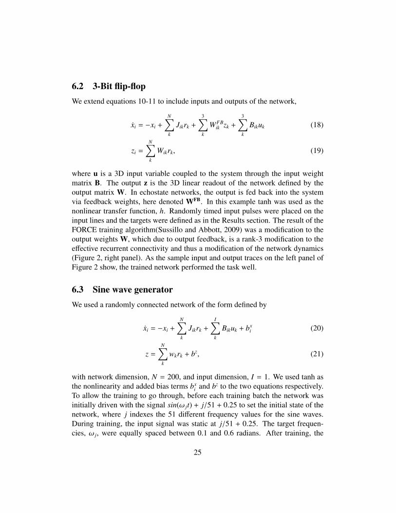
where u is a 3D input variable coupled to the system through the input weightmatrix B. The output z is the 3D linear readout of the network defined by theoutput matrix W. In echostate networks, the output is fed back into the systemvia feedback weights, here denoted WFB. In this example tanh was used as thenonlinear transfer function, h. Randomly timed input pulses were placed on theinput lines and the targets were defined as in the Results section. The result of theFORCE training algorithm(Sussillo and Abbott, 2009) was a modification to theoutput weights W, which due to output feedback, is a rank-3 modification to theeffective recurrent connectivity and thus a modification of the network dynamics(Figure 2, right panel). As the sample input and output traces on the left panel ofFigure 2 show, the trained network performed the task well.

6.3 Sine wave generatorWe used a randomly connected network of the form defined by

xi = −xi +

N∑k

Jikrk +

I∑k

Bikuk + bxi (20)

z =

N∑k

wkrk + bz, (21)

with network dimension, N = 200, and input dimension, I = 1. We used tanh asthe nonlinearity and added bias terms bx

i and bz to the two equations respectively.To allow the training to go through, before each training batch the network wasinitially driven with the signal sin(ω jt) + j/51 + 0.25 to set the initial state of thenetwork, where j indexes the 51 different frequency values for the sine waves.During training, the input signal was static at j/51 + 0.25. The target frequen-cies, ω j, were equally spaced between 0.1 and 0.6 radians. After training, the

25

1D network readout, z, successfully generated sin(ω jt) with only the static inputj/51+0.25 driving the network (no initial driving sinusoidal input was necessary).We trained the network to perform this task using the Hessian-Free optimizationtechnique for RNNs (Martens and Sutskever, 2011). The result of this trainingalgorithm was a modification to the matrices B, J, the vector w, as well as thebiases bx and bz.

6.4 2-Point moving averageThe network trained to implement the 2-point moving average was of the sameform as equations 20 and 21. The size of the network was 100 dimensions, withtwo inputs and one output. The first input contained randomly timed pulses lastingone second with each pulse taking a random value between -1 and 1, uniformly.The second input was an indicator variable, giving a pulse with value 1 wheneverthe first input was valid and was otherwise 0. The minimum time between pulseswas 5s, and the maximum was 30s. The target for the output was the averageof the last two input pulses. To minimally affect the dynamics, the target wasspecified for only a brief period before the next input pulse and was otherwiseundefined (see Figure 6 green traces.) The target was also defined to be zero at thebeginning of the simulation. This network was also trained using the Hessian-Freeoptimization technique for RNNs (Martens and Sutskever, 2011). The networkmean squared error was on the order of 1e-7.

For Figure 7 we selected the best local minima we could find by setting theoptimizer tolerance to 1e-27 with a maximum number of iterations set to 10000.This resulted in two ghosts/fixed points whose values were in the order of 1e-21.Given the potential for pathological curvature (Martens, 2010) in q in an examplewith a line or plane attractor, it’s possible that the two fixed points found areactually ghosts. However, the value of q at these two points is so small as to makeno practical difference between the two, so we refer to them as fixed points in themain text, since the dynamics are clearly structured by them.

We also selected slow points by varying the slow point acceptance (q value)between 1e-19 and 1e-4, with 200 attempts for a slow point per tolerance level.Slow points with q value greater than the tolerance were discarded. To visualizethe approximate plane attractor, we performed principal component analysis onthe slow points of the unperturbed system with q ≤ 1e-4. The subspace shown isthe first 3 principal components.

In the comparison of the LTVDS against the full RNN, we compared the tran-sitions of the current input to the last input (I1), and to the input before last (I0).

26

We decoded both I1 and I0 using the optimal linear projection found by regressingthe respective I0 or I1 values against the network activations across all trials.

The linear time varying dynamical system was defined as followed:

for t =1 to T , steps of ∆txs = closest slow point to x(t)

δx(t) = x(t) − xs

δx(t) = F′(xs) δx(t) + F(xs)

δx(t + ∆t) = δx(t) + ∆t δx(t)x(t + ∆t) = xs + δx(t + ∆t)

end,

where xs is the closest slow point to the current state and F′(xs) is the Jacobianaround that slow point. The set of potential xs was 2000 slow points from the2D manifold, found by setting the optimizer tolerances such that the q optimiza-tion found slow points with values just below 1e-10. This value was chosen as acompromise between the quality of the linearized system at the slow point, whichrequires a stringent q tolerance, and full coverage of the approximate plane attrac-tor, which requires a larger q tolerance. The transition simulations were initializedby choosing a random input pulse value for every slow point. Then the full RNNwas simulated for 1 second to correctly simulate the strong input. The networkstate at the end of the 1s was used as the IC for the comparison simulations ofboth the RNN and the LTVDS. The simulations were run for 20 seconds, allow-ing for equilibration to the 2D manifold for both the full RNN and the LTVDSapproximation.

For the perturbation experiments, we chose η values between 1e-7 and 0.1. Foreach value of η, we generated 50 perturbed networks where the perturbation waszero mean Gaussian noise with standard deviation η added to the recurrent weightmatrix. For each of the 50 networks, 1000 random examples were evaluated.The error for each η value was averaged across networks and examples. Theapproximate plane attractor shown in Figure 9D is with η = 0.006, a large ηvalue, but where the network still functioned with some drift.

7 AcknowledgementsWe thank Misha Tsodyks, Merav Stern, Stefano Fusi and Larry Abbott for helpfulconversations. DS was funded by NIH grant MH093338. OB was funded by the

27

Gatsby and Swartz Foundations and also by NIH grant MH093338.

ReferencesAhrens, M. B., Li, J. M., Orger, M. B., Robson, D. N., Schier, A. F., Engert, F., and

Portugues, R. (2012). Brain-wide neuronal dynamics during motor adaptationin zebrafish. Nature, 485(7399):471–477.

Bengio, Y., Simard, P., and Frasconi, P. (1994). Learning long-term dependen-cies with gradient descent is difficult. IEEE Transactions on Neural Networks,5(2):157–166.

Boyd, S. P. and Vandenberghe, L. (2004). Convex Optimization. Cambridge UnivPr.

Hopfield, J. and Tank, D. (1986). Computing with neural circuits: a model. Sci-ence, 233(4764):625–633.

Hopfield, J. J. (1982). Neural networks and physical systems with emergent col-lective computational abilities. Proceedings of the National Academy of Sci-ences of the United States of America, 79(8):2554–2558.

Huerta, R. and Rabinovich, M. (2004). Reproducible Sequence Generation InRandom Neural Ensembles. Physical Review Letters, 93(23):238104.

Jaeger, H. and Haas, H. (2004). Harnessing nonlinearity: predicting chaotic sys-tems and saving energy in wireless communication. Science, 304(5667):78–80.

Jones, L. M., Fontanini, A., Sadacca, B. F., Miller, P., and Katz, D. B. (2007).Natural stimuli evoke dynamic sequences of states in sensory cortical ensem-bles. Proceedings of the National Academy of Sciences of the United States ofAmerica, 104(47):18772–18777.

Liu, J. K. and Buonomano, D. V. (2009). Embedding multiple trajectories in sim-ulated recurrent neural networks in a self-organizing manner. J Neuroscience,29(42):13172–13181.

Maass, W., Joshi, P., and Sontag, E. D. (2007). Computational aspects of feedbackin neural circuits. PLoS Comput Biol, 3(1):e165.

28

Maass, W., Natschlager, T., and Markram, H. (2002). Real-time computing with-out stable states: a new framework for neural computation based on perturba-tions. Neural Computation, 14(11):2531–2560.

Machens, C. K., Romo, R., and Brody, C. D. (2005). Flexible control ofmutual inhibition: a neural model of two-interval discrimination. Science,307(5712):1121–1124.

Martens, J. (2010). Deep learning via Hessian-free optimization. In Proceedingsof the 27th International Conference on Machine Learning (ICML).

Martens, J. and Sutskever, I. (2011). Learning recurrent neural networks withhessian-free optimization. In Proceedings of the 28th International Conferenceon Machine Learning (ICML).

Ott, E. (2002). Chaos in Dynamical Systems. Cambridge Univ Pr.

Ponzi, A. and Wickens, J. (2010). Sequentially switching cell assemblies in ran-dom inhibitory networks of spiking neurons in the striatum. The Journal of neu-roscience : the official journal of the Society for Neuroscience, 30(17):5894–5911.

Rabinovich, M. I., Huerta, R., Varona, P., and Afraimovich, V. S. (2008). Transientcognitive dynamics, metastability, and decision making. PLoS Comput Biol,4(5):e1000072.

Romo, R., Brody, C. D., Hernandez, A., and Lemus, L. (1999). Neuronalcorrelates of parametric working memory in the prefrontal cortex. Nature,399(6735):470–473.

Rumelhart, D., Hinton, G., and Williams, R. (1985). Learning Internal Represen-tations by Error Propagation. Parallel Distributed Processing, 1:319–362.

Stopfer, M., Jayaraman, V., and Laurent, G. (2003). Intensity versus identitycoding in an olfactory system. Neuron, 39(6):991–1004.

Strogatz, S. H. (1994). Nonlinear Dynamics And Chaos. With Applications ToPhysics, Biology, Chemistry, And Engineering. Westview Pr.

Sussillo, D. and Abbott, L. F. (2009). Generating coherent patterns of activityfrom chaotic neural networks. Neuron, 63(4):544–557.

29

Wang, X. J. (2008). Decision making in recurrent neuronal circuits. Neuron,60(2):215–234.

30