Traveling wave dynamics for a one-dimensional

constrained Allen-Cahn equation

Goro Akagi(Mathematical Institute, Tohoku University)

Based on a joint work with

C. Kuehn (Munchen) and K.-I. Nakamura (Kanazawa)

Asia-Pacific Analysis and PDE Seminar

13 Sep 2021, The University of Sydney (via Zoom)

1. PDEs with non-decreasing

constraints

Non-decreasing constraints

In this talk, “non-decreasing constraints on evolution” mean

u(x, t) ≥ u(x, s) if t ≥ s,

or equivalently,

∂tu(x, t) ≥ 0.

Background: Irreversible Phase-field models (e.g., for brittle fracture)

Let u = u(x, t) denote a displacement field and z = z(x, t) a phase field,

which intuitively means

z(x, t) =

1 if the material is cracked at (x, t),

0 if the material is not cracked at (x, t).

Then t 7→ z(x, t) is supposed to be non-decreasing, unlike t 7→ u(x, t).1/46

Phase-field model for brittle fracture

The phase-field model reads,

0 = div(αε(z)∇u

)in Ω× R+,

∂tz =(ε∆z −

z

ε− α′

ε(z)|∇u|2)+

in Ω× R+,

which is an irreversible quasi-static evolution, i.e.,

0 = ∂uFε(u, z), ∂tz =(− ∂zFε(u, z)

)+,

of the free energy Fε(u, z) (= Ambrosio-Tortorelli regularization of the

Francfort-Marigo energy) given by

Fε(u, z) =1

2

∫Ω

αε(z)|∇u|2 dx+

∫Ω

(ε2|∇z|2 +

1

2εz2

)dx.

[Fremond-Nedjar ’96], [Bonetti-Schimperna ’04], [Mielke-Roubıcek ’08],

[Knees-Rossi-Zanini ’13-], [Takaishi-Kimura ’09,’11],...,[A-Schimperna ’21]2/46

Gradient flows with non-decreasing constraints

Let us focus on the gradient flow structure with non-decreasing constraints,

roughly speaking,

∂tu(t) =(− ∂J(u(t))

)+≥ 0

for some (possibly non-convex) functional J : X → R, say X = L2(Ω).

Equivalently, it can be rewritten as

∂tu(t) = −∂J(u(t)) − µ,

where µ can be characterized as

µ ∈ ∂I[0,+∞)(∂tu) and µ = −(− ∂J(u(t))

)−.

Stabilization ↔ Constraint

3/46

Aim of this talk

Address ourselves onto simpler PDEs with non-decreasing constraints and

discuss asymptotic behavior of solutions.

In particular, we shall discuss traveling wave dynamics for the 1D Allen-Cahn

equation with non-decreasing constraints,

(∗) ut =(uxx −W ′(u)

)+

in R× R+.

cf.) [A-Efendiev ’19] Cauchy-Dirichlet problem in bounded domains of RN

well-posedness, (partial) smoothing effect

energy-dissipation estimates, absorbing set, global attractor

reformulation of (∗) as an obstacle problem

convergence to equilibria as t→ +∞ and steady-state equation4/46

2. Traveling wave dynamics

Allen-Cahn equation in R

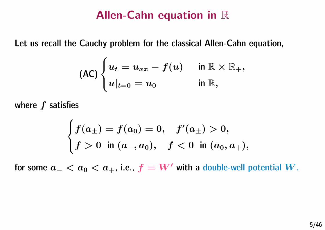
Let us recall the Cauchy problem for the classical Allen-Cahn equation,

(AC)

ut = uxx − f(u) in R× R+,

u|t=0 = u0 in R,

where f satisfiesf(a±) = f(a0) = 0, f ′(a±) > 0,

f > 0 in (a−, a0), f < 0 in (a0, a+),

for some a− < a0 < a+, i.e., f = W ′ with a double-well potential W .

5/46

Allen-Cahn equation in R

Let us recall the Cauchy problem for the classical Allen-Cahn equation,

(AC)

ut = uxx − f(u) in R× R+,

u|t=0 = u0 in R.

♠ phase separation model (e.g., binary alloy),

♠ L2 gradient flow of the free energy

J(u) :=1

2

∫R|∂xu(x)|2 dx+

∫RW (u(x)) dx

where W ′ = f . Namely,

(AC) ⇔ ut = −∂J(u) in L2(R), t > 0.

Hence t 7→ J(u(t)) is non-increasing.6/46

Traveling wave solutions for (AC)

The traveling wave solution u(x, t) = ϕ(x− ct) is characterized

by a profile function ϕ and a velocity constant c satisfying

−cϕ′ = ϕ′′ − f(ϕ) in R,

ϕ(ξ)→ a± as x→ ±∞

and

c

< 0 if W (a+) < W (a−),

= 0 if W (a−) = W (a+),

> 0 if W (a−) < W (a+).

-0.6

-0.5

-0.4

-0.3

-0.2

-0.1

0

0.1

-1.5 -1 -0.5 0 0.5 1

7/46

Traveling wave solutions for (AC)

[Fife-McLeod ’72]

Existence and “uniqueness” of TWs

Phase-plain analysis

Exponential stability of TWs: if

u0(x) ∈ [a−, a+], lim supx→−∞

u0(x) < a0, lim infx→+∞

u0(x) > a0,

then there exist constants x0 ∈ R, K,κ > 0 such that

‖u(·, t)− ϕ(· − ct− x0)‖L∞(R) ≤ Ke−κt for all t ≥ 0.

Schauder estimate, precompactness of u(·+ ct, t) : t ≥ 0,sub / supersolution method

[X. Chen ’92] Non-local reaction, Sub / supersolution method only8/46

Constrained Allen-Cahn equation

Now, we shall consider

(AC)+

ut =(uxx − f(u)

)+

in R× R+,

u|t=0 = u0 in R,

where f satisfiesf(a±) = f(a0) = 0, f ′(a±) > 0,

f > 0 in (a−, a0), f < 0 in (a0, a+)

for some a− < a0 < a+ and

(s)+ := maxs, 0 ≥ 0.

9/46

Constrained Allen-Cahn equation

Now, we shall consider

(AC)+

ut =

(uxx − f(u)︸ ︷︷ ︸

= − ∂J(u)

)+

in R× R+,

u|t=0 = u0 in R,

Then t 7→ J(u(t)) is still non-increasing.

Moreover, (AC)+ is equivalent to

ut = − ∂J(u) − µ, µ ∈ ∂I[0,+∞)(ut), u|t=0 = u0,

minu− u0 , ut − uxx + f(u) = 0, u|t=0 = u0

⇔ ut = − ∂J(u) − µ, µ ∈ ∂I[u0(x),∞)(u), u|t=0 = u0.

10/46

Traveling wave dynamics for (AC)+

We shall discuss

existence and uniqueness of traveling wave solutions,

convergence to a traveling wave solution.

In what follows, we may restrict ourselves to a balanced potential:

a± = ±1, a0 = 0, W (u) =1

4(u2 − 1)2,

for which the TW of (AC) fulfills

c = 0 and ϕ(±∞) = ±1.

11/46

3. Existence and uniqueness

of traveling waves

Balanced double-well potential

Balanced double-well potential W (u)12/46

Heuristic construction

Substitute u(x, t) = ϕ(x− ct) to (AC)+. Then a profile equation reads,

−cϕ′ =(ϕ′′ − f(ϕ)

)+.

How can we solve it ?

Instead, we shall derive an alternative profile equations...

13/46

Heuristic construction

Suppose that u(−∞) ≡ α ∈ (−1, 0), which is a steady-state for (AC)+.

(i) Due to the non-decreasing constraint ut ≥ 0,

u(x, t) ≥ α.

Then the region [u < α] on the graph of W (u) is prohibited.

(ii) Analogously to the reformulation, u may solve the obstacle problem,

ut − uxx + f(u)︸ ︷︷ ︸=W ′(u)

+ ∂I[α,+∞)(u) 3 0 in R× R.

Roughly speaking,

W ′(u) + ∂I[α,+∞)(u) = ∂(W + I[α,+∞)︸ ︷︷ ︸

truncation !

)(u).

14/46

Heuristic construction

Truncated balanced double-well potential W (u)

15/46

Profile equation for traveling waves

Let α ∈ (−1, 0) and substitute u = ϕ(x− ct). Then

(∗) − cϕ′ − ϕ′′ +W ′(ϕ) + ∂I[α,∞)(ϕ)︸ ︷︷ ︸= ∂(W+I[α,∞))(ϕ)

3 0 in R

is derived along with

ϕ(−∞) = α and ϕ(+∞) = 1 and ϕ′ ≥ 0

as a profile equation.

Indeed, let ϕα be a solution of (∗) for some c = cα.

Then u(x, t) = ϕα(x− cαt) solves (AC)+

and cα < 0 if α 6= −1.16/46

Existence of traveling wave solutions

17/46

Existence of traveling wave solutions

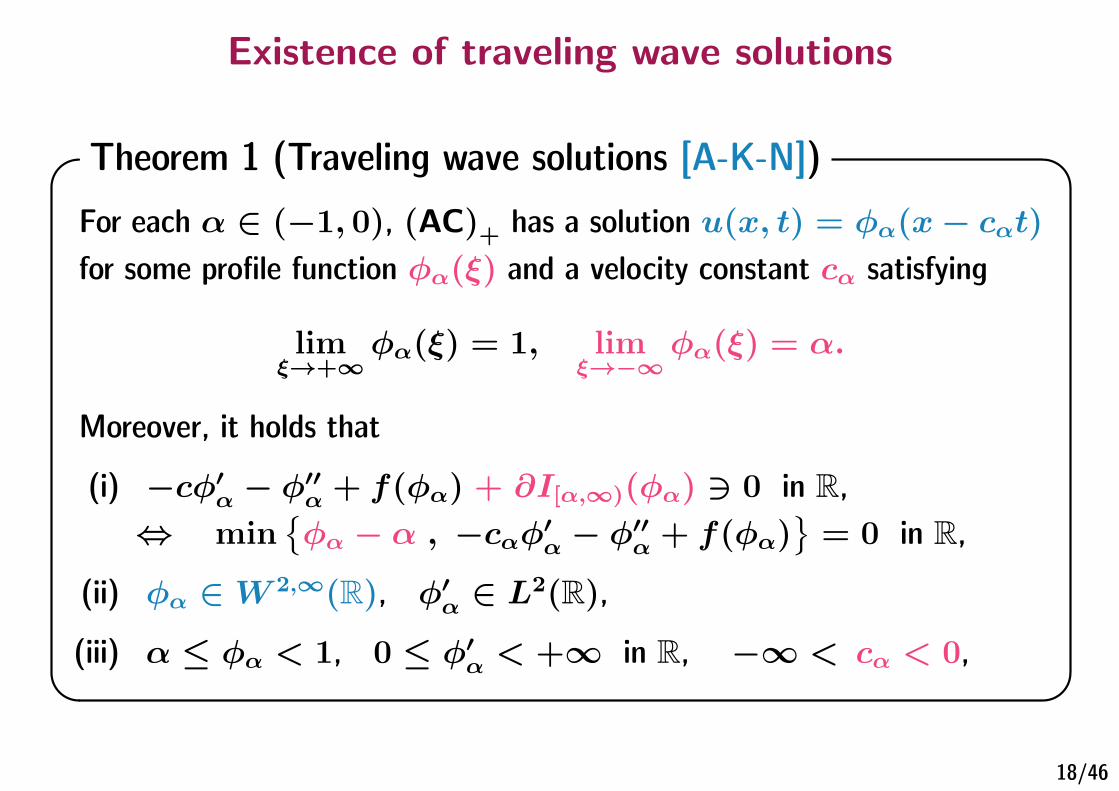
Theorem 1 (Traveling wave solutions [A-K-N]) For each α ∈ (−1, 0), (AC)+ has a solution u(x, t) = ϕα(x− cαt)for some profile function ϕα(ξ) and a velocity constant cα satisfying

limξ→+∞

ϕα(ξ) = 1, limξ→−∞

ϕα(ξ) = α.

Moreover, it holds that

(i) −cϕ′α − ϕ′′

α + f(ϕα) + ∂I[α,∞)(ϕα) 3 0 in R,⇔ min

ϕα − α , −cαϕ′

α − ϕ′′α + f(ϕα)

= 0 in R,

(ii) ϕα ∈W 2,∞(R), ϕ′α ∈ L2(R),

(iii) α ≤ ϕα < 1, 0 ≤ ϕ′α < +∞ in R, −∞ < cα < 0,

18/46

Existence of traveling wave solutions

Theorem 1 (Traveling wave solutions [A-K-N] (contd.)) There exists s0 ∈ R such that

ϕα(s) = α on (−∞, s0], ϕα(s) > α on (s0,∞).

Furthermore, −cαϕ′α − ϕ′′

α + f(ϕα) = 0 in (s0,+∞), and hence,

ϕ′′α(s0 − 0) = 0 and ϕ′′

α(s0 + 0) = f(α) > 0,

which implies ϕ 6∈ C2(R). In what follows, we set s0 = 0 by translation. Hence

ϕα = α on (−∞, 0], ϕα > α on (0,∞).

19/46

Existence of traveling wave solutions

20/46

Uniqueness of profile and velocity

Theorem 2 (Uniqueness of traveling waves [A-K-N]) Concerning traveling wave solutions discussed in Theorem 1, it holds that

(i) the velocity cα is unique for each α,

(ii) the profile function ϕα is unique (up to translation) for each α.

21/46

4. Convergence to

traveling waves

Question

Question Can we also prove the (exponential) convergence of solutions for (AC)+to traveling waves as in the classical Allen-Cahn equation ?

We cannot expect stability of traveling wave solutions.

Proposition 3 (Instability of traveling waves [A-K-N]) For each α ∈ (a−, a0), the traveling wave solution ϕα(x − cαt) of

(AC)+ is unstable in L∞(R). Hence the basin of attraction of the traveling wave solution for (AC)+ is

smaller than those for (AC).

22/46

Hypotheses for initial data

For α ∈ (a−, a0), we assume (with a± = ±1 and a0 = 0):

(H)α

u0 ∈ H2

loc(R), lim infx→+∞

u0(x) > a0,

a− ≤ infx∈R

u0(x) ≤ supx∈R

u0(x)< a+,

u0 ≡ α on (−∞, ξ1] for some ξ1 ∈ R.

Then one can define

r(t) := supr ∈ R : u(x, t) = α for all x ≤ r ∈ R for t ≥ 0.23/46

Main result

Theorem 4 (Exponential convergence to a TW [A-K-N]) Let α ∈ (a−, a0) be such that f ′(α) > 0 and assume that u0 satisfies

(H)α. Let u = u(x, t) be the L2loc solution to (AC)+ for the initial

datum u0. Then there exist x0 ∈ R and K,κ > 0 such that

‖u(·, t)− ϕα(· − cαt− x0)‖L∞(R) ≤ Ke−κt for all t ≥ 0.

Set r(t) := supr > 0: u(·, t) ≡ α on (−∞, r]. Then

|r(t)− cαt− x0| ≲ e−κ2t as t→ +∞.

24/46

Supersolutions of (AC)+ cannot decrease !

We note that

Ut ≥(Uxx − f(U)

)+≥ 0

implies

U(x, t) cannot decrease in time !

Hence the sub- and supersolution method does not work well for (AC)+(cf. Fife-McLeod & Chen).

⇒ Our proof consists of “4 phases”.

25/46

Rough outline of proof

Phases 1 & 2 Reduction to a simplified system

Reduction to a constant obstacle problem There exists t1 > 0 such that, for all t ≥ t1,

u(x, t) = u0(x) if and only if u(x, t) = α.

Hence (AC)+ is reduced to

(AC)α min u− α , ut − uxx + f(u) = 0 in R. Phase 3 Quasi-convergence of the orbit O = u( · + cαt, t) : t ≥ t1

to the limit ϕα( · − x0) unif. in R for some x0 ∈ R Energy method

Phase 4 Exponential convergence of u(·, t) to ϕα(· − cαt− x0)

uniformly in R as t→ +∞ Sub- and supersolution method

26/46

Initial Phase

♠ Initial Phase

Claim ∃t1 > 0 ; inf

x∈Ru(x, t1) > a−.

Let uac be the unique solution to (AC) with the same datum u0. Moreover,

ut =(uxx − f(u)

)+≥ uxx − f(u) in R× R+.

By comparison principle,

u(x, t) ≥ uac(x, t)→ ϕac(x) as t→ +∞,

where ϕac is a TW with c = 0 connecting a± at x = ±∞.

27/46

Initial Phase

Let uac(x, t) be the solution to (AC) with uac(x, 0) = u0(x).

28/46

Initial Phase

Let uac(x, t) be the solution to (AC) with uac(x, 0) = u0(x).

28/46

Initial Phase

Then uac(x, t) converges to a layer solution ϕac(x) (with c = 0).

29/46

Initial Phase

The solution u(x, t) of (AC)+ is a supersolution to (AC).

Hence u(x, t) ≥ uac(x, t).

30/46

Second Phase

♠ Second Phase

Lemma 5 (Reduction to a constant obstacle problem) There exists t2 > t1 such that, for all t > t2,

u(x, t) = u0(x) ⇔ u(x, t) = α. We employ a subsolution to (AC)+ given by

Uγ(x, t) := ϕγ(x− cγt−σδ(1− e−βt)− h−)− δe−βt

for some h− ∈ R, β, δ, σ > 0 and γ ∈ (a−, a0) satisfying

a− < γ − δ < infx∈R

u(x, t1).

Then we assure that cγ < 0.31/46

Second Phase

a+

a0

a-

u(x,t)

infx∈R

u(x, t1) > a−

32/46

Second Phase

a+

a0

a-

u(x,t+s)

U (x,s),

C < 0

Eventually, u(x, t+ s) ≥ Uβ,γ(x, s) > α = u0(x) for all x ≥ ξ1.Therefore u(x, t) = u0(x) ⇔ u(x, t) = α.

33/46

Second Phase

Thanks to the reformulation, we assure that

(AC)+ ⇔ (AC)α min u− α, ut − uxx + f(u) = 0 in R

for all t > t2.

34/46

Third Phase

♠ Third Phase

Lemma 6 (Quasi-convergence of u(· − cαt, t)) There exist a sequence tn → +∞ and ξ ∈ R such that

‖u(·, tn)− ϕα(· − cαtn + ξ)‖L∞(R) → 0. We prove the precompactness of u(· − cαt, t) : t > t2 in H1

loc(R) by

developing local energy estimates for (AC)α and identify the limit of the

orbit.

Thereby, for any δ > 0 (small), one can take nδ ∈ N such that

ϕα(x− cαtnδ)− δ ≤ u(x, tnδ

) ≤ ϕα(x− cαtnδ) + δ

for any x ∈ R (after a suitable translation).35/46

Third Phase

Set

v(y, t) := u(y + cαt, t)− a+ ∈ [α− a+, 0], y ∈ R+, t > t2.

Then (AC)α implies

∂tv − ∂2yv + η + f(v + a+) = cα∂yv, η ∈ ∂I[α,∞)(v + a+)

in R+ × R+. We can assume WLOG (by translation) that

v(0, t) = α− a+, ∂yv(0, t) = 0, v(y, 0) = u(y, 0).

A key step is to establish local-energy estimates for v(y, t).

Step 1 Based on [A-Efendiev ’19], we can prove that

supt≥0

∫R|η(·, t)|2ρ dx ≤

∫R|(∂2

xu0 − f(u0))−|2ρ dx ∀ρ ∈ C∞c (R).

36/46

Third Phase

Step 2 (Caccioppoli type estimate) Let ζR ∈ C∞c (R) be such that

ζR ≡ 1 in [0, R], ζR ≡ 0 in [2R,+∞), ‖ζ′R‖L∞(R+) ≤2

R.

Test (AC)α by e−λtecαyvζ2R. Then

1

2e−2λt

∫ +∞

0ecαyv(·, t)2ζ2R dy +

1

2

∫ t

0e−2λτ

(∫ +∞

0ecαy|∂yv|2ζ2R dy

)dτ

≤1

2|cα|‖v(·, 0)‖2L∞(R+) +

4

λ|cα|R2‖v‖2L∞(QT ),

where we used the fact that f ′′ ≥ −λ and vη ≥ 0. Let R→ +∞. Then∫ t

0

e−2λτ

(∫ +∞

0

ecαy|∂yv|2 dy)dτ ≤ C.

37/46

Third Phase

Step 3 (Weighted energy estimate for ∂tv) Test (AC)α by ecαy∂tv. Then∫ ∞

0ecαy|∂tv|2 dy +

d

dt

(1

2

∫ ∞

0ecαy|∂yv|2 dy +

∫ ∞

0ecαyh(v) dy︸ ︷︷ ︸

=E(v(·,t))

)= 0.

where h(v) = f(v + a+) ≥ 0, since η∂tv ≡ 0 by η ∈ ∂I[0,+∞)(∂tu).

Integrate it over (τ0, t) with τ0 > 0. It then follows from Step 1 that∫ t

τ0

∫ ∞

0

ecαy|∂tv(y, τ )|2 dydτ + E(v(·, t)) ≤ E(v(·, τ0)) ∀t ≥ τ0.

Step 4 (Quasi-convergence local in space) One can take tn →∞ such that

∂tv(·, tn)→ 0 strongly in L2(R+; ecαydy),

38/46

Third Phase

η(·, tn)→ η∞ weakly in L2(0, R),

v(·, tn)→ ψ weakly in H2(0, R),

strongly in C1([0, R])

for some ψ ∈ H2loc(R+) and any R > 0. Set

ϕ(y) =

ψ(y) + a+ if y ≥ 0,

α if y < 0,

which then solves

−ϕ′′ + f(ϕ) + I[α,∞)(ϕ) 3 cαϕ′ in R, ϕ(0) = α, ϕ′(0) = 0.

Claim: ∃h1 ∈ R such that ϕ(x) = ϕα(x− h1) ∀x ∈ R.

39/46

Third Phase

Thus there exists a sequence tn → +∞ such that

supy≤R

|u(y + cαtn, tn)− ϕα(y − h1)| → 0 for R > 0.

Step 5 (Quasi-convergence global in space)

Recall Uγ and ϕα and use comparison argument to

|u(y+cαtn, tn)−ϕα(y−h1)| ≤ a+−minu(y+cαtn, tn), ϕα(y−h1).

40/46

Final Phase

♠ Final Phase Modifying the argument in [X. Chen ’92], we shall prove

exponential convergence of u(·, t) to ϕα(· − cαt) over R as t→ +∞(without taking any subsequence). Set

w±(x, t) := ϕα(x− cαt±σδ(1− e−βt)− h±)± δe−βt

for h± ∈ R, δ ∈ (0, δ0) and β, σ > 0. Then w± turns out to be a super-

and a subsolution to (AC)α, provided δ0, β, σ are small enough.

Lemma 7 (Enclosing) Set h+ = 0 and assume ϕα(·−h−)−δ ≤ u(·, 0) ≤ ϕα(·)+δ in R.If δ ∈ (0, δ0) and h− ≥ 0 are small enough, one can take ε ∈ (0, 1)

and t 1 such that

ϕα(x−cαt−ε(h−−δ))−εδ ≤ u(x, t) ≤ ϕα(x−cαt+εδ)+εδ. 41/46

Final Phase

δ

(AC)

w+

w-

u

By comparison principle, w−(x, t) ≤ u(x, t) ≤ w+(x, t).

42/46

Final Phase

δ

(AC)

w+

w-

u

Set W± := ±(w± − u) ≥ 0. Then

∂tW± − ∂2

xW± ≥ ∓

(f(w±)− f(u)

)≥ −MW±.

By strong maximum principle, one has W+ ≥ ∃c0 > 0 or W− ≥ c0 > 0.43/46

Final Phase

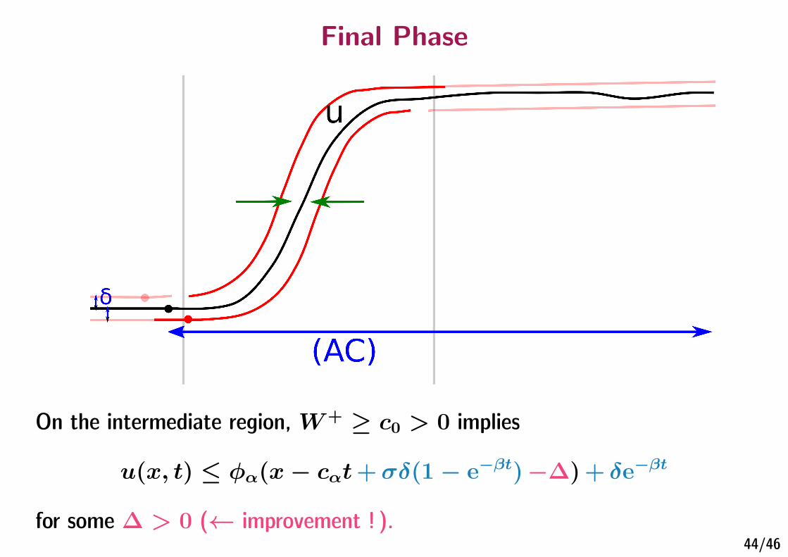
On the intermediate region, W+ ≥ c0 > 0 implies

u(x, t) ≤ ϕα(x− cαt+σδ(1− e−βt)−∆)+ δe−βt

for some ∆ > 0 (← improvement ! ).44/46

Final Phase

If ϕ′α 1, one can then enclose u(x, t) with smaller error:

ϕα(x− cαt) ≈ ϕα(x− cαt −∆)−∆ϕ′α(x− cαt)

On the left region, 0 < r0 < h− should be small enough.45/46

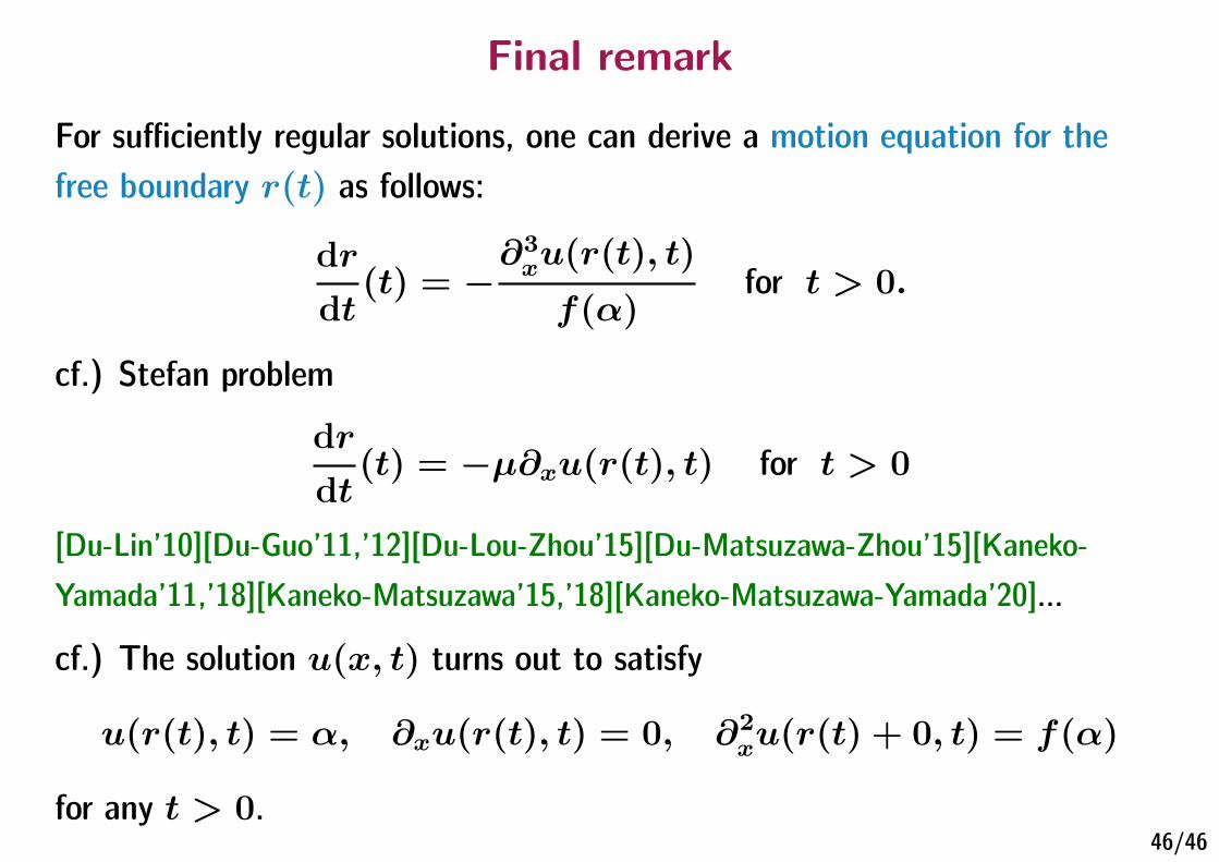
Final remark

For sufficiently regular solutions, one can derive a motion equation for the

free boundary r(t) as follows:

dr

dt(t) = −

∂3xu(r(t), t)

f(α)for t > 0.

cf.) Stefan problem

dr

dt(t) = −µ∂xu(r(t), t) for t > 0

[Du-Lin’10][Du-Guo’11,’12][Du-Lou-Zhou’15][Du-Matsuzawa-Zhou’15][Kaneko-

Yamada’11,’18][Kaneko-Matsuzawa’15,’18][Kaneko-Matsuzawa-Yamada’20]...

cf.) The solution u(x, t) turns out to satisfy

u(r(t), t) = α, ∂xu(r(t), t) = 0, ∂2xu(r(t) + 0, t) = f(α)

for any t > 0.46/46

Thank you for your attention !

Goro AkagiTohoku University, JPgoro.akagi@tohoku.ac.jp