openair News News The openair Project newsletter Issue 12, May 2012 Special issue on the use of...

OPEN sourc

e

openair NewsThe openair Project newsletter Issue 12, May 2012

Special issue on the use of cluster analysisin openairThere have been several recent developments inopenair related to the use of cluster analysis as atool for understanding air pollution. This newsletterfocuses on the use of two complementary functions:polarCluster and trajCluster.

polarCluster is a new function (and approach)that is used with the polarPlot function. ThepolarPlot function often reveals interesting pat-terns in data that help to diUerentiate diUerent sourcetypes or characteristics. So far the focus on usingthe polarPlot function has been as a graphical toolrather than a quantitative one. The ‘problem’ hasbeen that while interesting features could be identi-Ved, the post processing of these features was some-what arbitrary and seldom carried out eUectively.The polarCluster provides more of a quantitativemeans of detecting interesting features that can thenbe post-processed using other openair functions.

The trajCluster function aims to clusterback trajectories and is in some ways similar to

polarCluster but is more relevant to the regionalscale. openair has a means of calculating back tra-jectories at pre-speciVed locations using the NOAAHYSPLIT model. It can be very useful to group tra-jectories by their geographic origin and post-processthese groups to identify diUerent chemical character-istics.

This newsletter introduces these two new func-tions and provides examples of their usage. Bothfunctions should help with analysing air pollutiondata in more detail and in particular identifying inter-esting features/air-masses that can easily be analysedand compared.

This newsletter was produced using R ver-sion 2.15.0 and openair version 0.6-0. To up-date to the most recent version of openair, typeupdate.packages() and make sure you are usingthe most recent version of R.

mailto:[email protected]

Contents

Special issue on the use of cluster analysis inopenair . . . . . . . . . . . . . . . . . . . 1

Cluster analysis with bivariate polar plots . . 2Cluster analysis of back trajectories . . . . . 5Other openair developments . . . . . . . . . 8

mailto:[email protected]

Issue 12, May 2012 2

Cluster analysis with bivariate polar plotsThe polarPlot function will often identify interest-ing features that would be useful to analyse further,such as those shown in Figure 1. It is possible toselect areas of interest based only on a considerationof a plot. Such a selection could be based on winddirection and wind speed intervals for example e.g.

subdata <- subset(mydata, ws > 3 &

wd >= 180 & wd <= 270)

polarPlot(mydata, pollutant = "so2")

0

5

10 wind spd.

15

20

25

W

S

N

E

mean

SO2

1

2

3

4

5

6

7

8

Figure 1: Example plots using the polarPlot func-tion for the mean concentration of SO2.

which would select wind speeds >3 /ms andwind directions from 180 to 270 degrees from mydata.That subset of data, subdata, could then be analysedusing other functions. While this approach maybe useful in many circumstances it is rather arbit-rary. In fact, the choice of “interesting feature” in theVrst place can even depend on the colour scale used,which is not very robust. Furthermore, many inter-esting patterns can be diXcult to select and won’talways fall into convenient intervals of other vari-ables such as wind speed and direction.

A better approach is to use a method that canselect group similar features together. One such ap-proach is to use cluster analysis. openair uses k-means clustering as a way in which bivariate polarplot features can be identiVed and grouped. Themain purpose of grouping data in this way is toidentify records in the original time series data bycluster to enable post-processing to better under-stand potential source characteristics. The processof grouping data in k-means clustering proceeds asfollows. First, k points are randomly chosen formthe space represented by the objects that are beingclustered into k groups. These points represent ini-

tial group centroids. Each object is assigned to thegroup that has the closest centroid. When all objectshave been assigned, the positions of the k centroidsis re-calculated. The previous two steps are repeateduntil the centroids no longer move. This produces aseparation of the objects into groups from which themetric to be minimised can be calculated.

Central to the idea of clustering data is theconcept of distance i.e. some measure of similar-ity or dissimilarity between points. Clusters shouldbe comprised of points separated by small distancesrelative to the distance between the clusters. Care-ful consideration is required to deVne the distancemeasure used because the eUectiveness of cluster-ing itself fundamentally depends on its choice. Thesimilarity of concentrations shown in Figure 1 forexample is determined by three variables: the u andv wind components and the concentration. All threevariables are equally important in characterising theconcentration-location information, but they exist ondiUerent scales i.e. a wind speed-direction measureand a concentration. The basic k-means algorithm is:

k∑j=1

n∑i=1

||x (j)i − cj ||2 (1)

where ||x (j)i − cj ||2 is a chosen distance measure

between a data point x (j)i and the cluster centre cj , isan indicator of the distance of the n data points fromtheir respective cluster centres.

The distance measure is deVned as the Euclideandistance:

dx ,y =

√√√√ J∑j=1

(xj − yj)2 (2)

Where x and y are two J-dimensional vectors,which have been standardized by subtracting themean and dividing by the standard deviation. In thecurrent case J is of length three i.e. the wind com-ponents u and v and the concentration C , each ofwhich is standardized e.g.:

xj =

(xj − x̄

σx

)(3)

Standardization is necessary because the windcomponents u and v are on diUerent scales to the con-centration. In principle, more weight could be givento the concentration rather than the u and v compon-ents, although this would tend to identify clusters

openairAn R package for air pollution data analysis


with similar concentrations but diUerent source ori-gins.

polarCluster can be thought of as the “local”version of clustering of back trajectories. Rather thanusing air mass origins, wind speed, wind directionand concentration are used to group similar condi-tions together.

The use of the polarCluster is very similar tothe use of all openair functions. While there aremany techniques available to try and Vnd the op-timum number of clusters, it is diXcult for theseapproaches to work in a consistent way for identify-ing features in bivariate polar plots. For this reasonit is best to consider a range of solutions that coversa number of clusters.

Cluster analysis is computationally intensive andthe polarCluster function can take a comparat-ively long time to run. The basic idea is to calculatethe solution to several cluster levels and then chooseone that oUers the most appropriate solution for post-processing.

The example given below is for concentrationsof SO2, shown in Figure 1 and the aim is to identifyfeatures in that plot. A range of numbers of clusterswill be calculated — in the is case from two to ten.

polarCluster(mydata, pollutant = "so2",n.clusters = 2:10, cols = "Set3")

0 5

10 wind spd. 15

20 25

W

S

N

E

2 clusters

0 5

10 wind spd. 15

20 25

W

S

N

E

3 clusters

0 5

10 wind spd. 15

20 25

W

S

N

E

4 clusters

0 5

10 wind spd. 15

20 25

W

S

N

E

5 clusters

0 5

10 wind spd. 15

20 25

W

S

N

E

6 clusters

0 5

10 wind spd. 15

20 25

W

S

N

E

7 clusters

0 5

10 wind spd. 15

20 25

W

S

N

E

8 clusters

0 5

10 wind spd. 15

20 25

W

S

N

E

9 clusters

0 5

10 wind spd. 15

20 25

W

S

N

E

10 clusters

cluster12345678910

Figure 2: Use of the polarCluster function appliedto SO2 concentrations at Marylebone Road. In thiscase 2 to 10 clusters have been chosen.



results <- polarCluster(mydata, pollutant ="so2",

n.clusters = 8, cols = "Set3")

0

5

10 wind spd.

15

20

25

W

S

N

E

cluster12345678

Figure 3: Use of the polarCluster function appliedto SO2 concentrations at Marylebone Road. In thiscase 8 clusters have been chosen.

The real beneVt of polarCluster is being ableto identify clusters in the original data frame. To dothis, the results from the analysis must be read intoa new variable, as in Figure 3, where the results areread into a data frame results. Now it is possibleto use this new information. In the 8-cluster solutionto Figure 3, cluster 6 seems to capture the elevatedSO2 concentrations to the east well (see Figure 1 forcomparison), while cluster 5 will strongly representthe road contribution.

The results are here:

head(results$data)

## date ws wd nox no2 o3## 1 1998-01-01 00:00:00 0.60 280 285 39 1## 2 1998-01-01 02:00:00 2.76 190 NA NA 3## 3 1998-01-01 03:00:00 2.16 170 493 52 3## 4 1998-01-01 04:00:00 2.40 180 468 78 2## 5 1998-01-01 05:00:00 3.00 190 264 42 0## 6 1998-01-01 06:00:00 3.00 140 171 38 0## pm10 so2 co pm25 cluster## 1 29 4.723 3.373 NA 5## 2 34 6.830 9.602 NA 5## 3 35 7.662 10.217 NA 4## 4 34 8.070 8.912 NA 4## 5 16 5.505 3.053 NA 5## 6 11 4.230 2.265 NA 4

Note that there is an additional column clusterthat gives the cluster a particular row belongs to andthat this is a character variable. It might be easier to

read these results into a new data frame:

results <- results$data

It is easy to Vnd out how many points are in eachcluster:

table(results$cluster)

#### 1 2 3 4 5 6 7## 194 484 156 15994 24782 2370 7677## 8## 3066

Now other openair analysis functions can beused to analyse the results. For example, to considerthe temporal variations by cluster:

timeVariation(results, pollutant = "so2",group = "cluster", col = "Set3", ci = FALSE,lwd = 3)

Or if we just want to plot a couple of clusters (5and 6) using the same colours as in Figure 3:

timeVariation(subset(results, cluster %in%c("5", "6")), pollutant = "so2", group =

"cluster",col = openColours("Set3", 8)[5:6], lwd = 3)

hour

SO

2

5

10

15

20

0 6 12 18 23

Monday

0 6 12 18 23

Tuesday

0 6 12 18 23

Wednesday

0 6 12 18 23

Thursday

0 6 12 18 23

Friday

0 6 12 18 23

Saturday

0 6 12 18 23

Sunday

5 6

hour

SO

2

4

6

8

10

12

0 6 12 18 23

month

SO

2

5

6

7

8

9

J F M A M J J A S O N D

weekday

SO

2

5

6

7

8

9

10

Mon Tue Wed Thu Fri Sat Sun

Figure 4: Use of the timeVariation function toshow the temporal components of the clusters iden-tiVed in Figure 3.

polarClusterwill work on any surface that canbe plotted by polarPlot e.g. the radial variable doesnot have to be wind speed but could be another vari-able such as temperature. While it is not alwayspossible for polarCluster to identify all features ina surface it certainly makes it easier to post-processpolarPlots using other openair functions or in-deed other analyses altogether.



Cluster analysis of back trajectoriesOften it is useful to use cluster analysis on back tra-jectories to group similar air mass origins together.The principal purpose of clustering back trajectoriesis to post-process data according to cluster origin.By grouping data with similar geographic origins itis possible to gain information on pollutant specieswith similar chemical histories. There are severalways in which clustering can be carried out and sev-eral measures of the similarity of diUerent clusters.A key issue is how the distance matrix is calculated,which determines the similarity (or dissimilarity) ofdiUerent back trajectories. The simplest measure isthe Euclidean distance. However, an angle-basedmeasure is also often used. The two distance meas-ures are deVned below. In openair the distancematrices are calculated using C++ code becausetheir calculation is computationally intensive. Notethat these calculations can also be performed directlyin the HYSPLIT model itself.

The Euclidean distance between two trajectoriesis given by Equation 1. Where X1, Y1 and X2, Y2

are the latitude and longitude coordinates of backtrajectories 1 and 2, respectively. n is the number ofback trajectory points (96 hours in this case).

d1,2 =

√√√√ n∑i=1

((X1i − X2i )2 + (Y1i − Y2i ))2 (1)

The angle distance matrix is a measure of howsimilar two back trajectory points are in terms oftheir angle from the origin i.e. the starting locationof the back trajectories. The angle-based measurewill often capture some of the important circulat-ory features in the atmosphere e.g. situations wherethere is a high pressure located to the east of the UK.However, the most appropriate distance measure willbe application dependent and is probably best testedby the extent to which they are able to diUerentiatediUerent air-mass characteristics, which can be testedthrough post-processing. The angle-based distancemeasure is deVned as:

d1,2 =1

n

n∑i=1

cos−1

(0.5

Ai + Bi + Ci√AiBi

)(2)

where

Ai = (X1(i)− X0)2 + (Y1(i)− Y0)2 (3)

Bi = (X2(i)− X0)2 + (Y2(i)− Y0)2 (4)

Ci = (X2(i)− X1(i))2 + (Y2(i)− Y1(i))2 (5)

where X0 and Y0 are the coordinates of the loc-ation being studied i.e. the starting location of thetrajectories.

As an example we will consider back trajectoriesfor London in 2011.

First, the back trajectory data for London is im-ported together with the air pollution data for theNorth Kensington site (KC1).

traj <- importTraj(site = "london",year = 2011)

kc1 <- importKCL(site = "kc1", year = 2011)

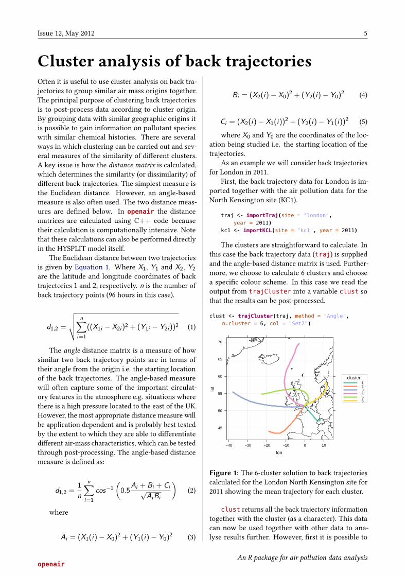
The clusters are straightforward to calculate. Inthis case the back trajectory data (traj) is suppliedand the angle-based distance matrix is used. Further-more, we choose to calculate 6 clusters and choosea speciVc colour scheme. In this case we read theoutput from trajCluster into a variable clust sothat the results can be post-processed.

clust <- trajCluster(traj, method = "Angle",n.cluster = 6, col = "Set2")

lon

lat

45

50

55

60

65

70

−40 −30 −20 −10 0 10

cluster 1 2 3 4 5 6

Figure 1: The 6-cluster solution to back trajectoriescalculated for the London North Kensington site for2011 showing the mean trajectory for each cluster.

clust returns all the back trajectory informationtogether with the cluster (as a character). This datacan now be used together with other data to ana-lyse results further. However, Vrst it is possible to



show all trajectories coloured by cluster, althoughfor a year of data there is signiVcant overlap and it isdiXcult to tell them apart.

trajPlot(clust, group = "cluster",plot.type = "l")

Perhaps more useful is to merge the cluster datawith measurement data. In this case the data at NorthKensington site are used. Note that in merging thesetwo data frames it is not necessary to retain all 96back trajectory hours and for this reason we extractonly the Vrst hour.

kc1 <- merge(kc1, subset(clust, hour.inc ==0), by = "date")

Now kc1 contains air pollution data identiVed bycluster. The size of this data frame is about a thirdof the original size because back trajectories are onlyrun every 3 hours.

The numbers of each cluster are given by:

table(kc1$cluster)

#### 1 2 3 4 5 6## 347 661 989 277 280 333

i.e. is dominated by clusters 3 and 2 from westand south-west (Atlantic).

Now it is possible to analyse the concentrationdata according to the cluster. There are numeroustypes of analysis that can be carried out with theseresults, which will depend on what the aims of theanalysis are in the Vrst place. However, perhaps oneof the Vrst things to consider is how the concentra-tions vary by cluster. As the summary results belowshow, there are distinctly diUerent mean concentra-tions of most pollutants by cluster. For example,clusters 1 and 6 are associated with much higher con-centrations of PM10— approximately double that ofother clusters. Both of these clusters originate fromcontinental Europe. Cluster 5 is also relatively high,which tends to come from the rest of the UK. Otherclues concerning the types of air-mass can be gainedfrom the mean pressure. For example, cluster 5 is as-sociated with the highest pressure (1014 kPa), and asis seen in Figure 1 the shape of the line for cluster 5is consistent with air-masses associated with a highpressure system (a clockwise-type sweep).

ddply(kc1, .(cluster), numcolwise(mean),na.rm = TRUE)

## cluster nox no2 o3 so2 co## 1 1 89.89 51.37 32.86 3.345 0.3884## 2 2 40.89 30.93 39.58 1.249 0.2229## 3 3 47.15 32.30 39.84 1.721 0.1889## 4 4 44.09 30.64 40.06 1.728 0.1884## 5 5 57.00 39.16 41.43 2.124 0.2263## 6 6 64.88 42.38 46.40 2.837 0.2895## pm10_raw pm10 pm25 v2.5 nv2.5 receptor## 1 32.34 35.82 31.35 8.015 23.330 1## 2 18.12 17.70 11.55 3.131 8.419 1## 3 19.40 17.86 11.26 2.801 8.461 1## 4 19.80 17.60 10.99 2.172 8.816 1## 5 24.38 25.49 16.52 4.498 12.025 1## 6 31.71 35.72 29.73 7.569 22.147 1## year month day hour hour.inc lat lon## 1 2011 7.660 15.28 10.12 0 51.5 -0.1## 2 2011 6.268 15.45 10.59 0 51.5 -0.1## 3 2011 7.470 15.75 10.41 0 51.5 -0.1## 4 2011 6.863 17.76 10.97 0 51.5 -0.1## 5 2011 5.225 16.13 10.12 0 51.5 -0.1## 6 2011 4.381 15.80 10.88 0 51.5 -0.1## height pressure len## 1 10 1005 97## 2 10 1005 97## 3 10 1006 97## 4 10 1007 97## 5 10 1014 97## 6 10 1011 97

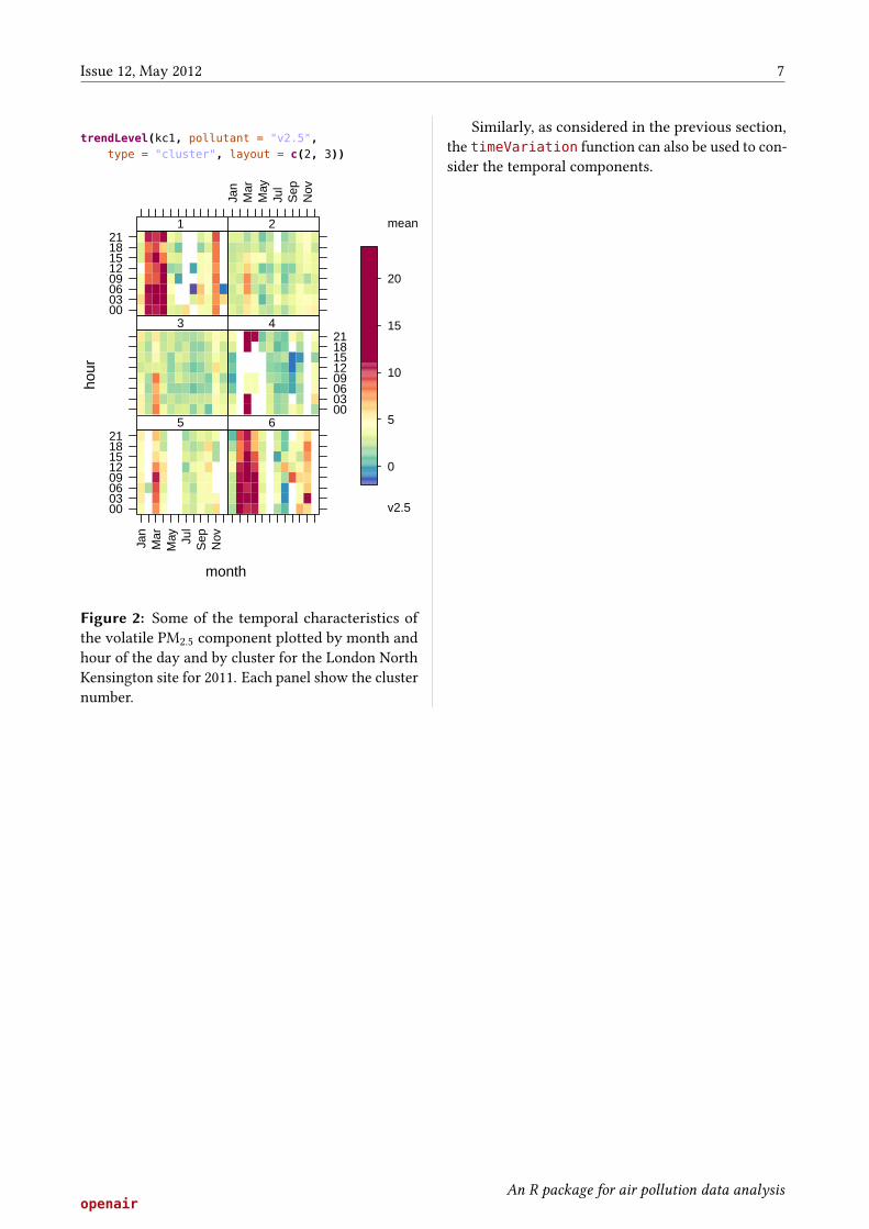
Simple plots can be generated from these resultstoo. For example, it is easy to consider the temporalnature of the volatile component of PM2.5 concen-trations (v2.5 in the kc1 data frame). Figure 2 forexample shows how the concentration of the volatilecomponent of PM2.5 concentrations varies by clusterby plotting the hour of day-month variation. It isclear from Figure 2 that the clusters associated withthe highest volatile PM2.5 concentrations are clusters1 and 6 (European origin) and that these concentra-tions peak during spring. There is less data to seeclearly what is going on with cluster 5. Nevertheless,the cluster analysis has clearly separated diUerent airmass characteristics which allows for more reVnedanalysis of diUerent air-mass types.



trendLevel(kc1, pollutant = "v2.5",type = "cluster", layout = c(2, 3))

month

hour

0003060912151821

1 Ja

nM

arM

ayJu

lS

epN

ov

2

3

0003060912151821

4

0003060912151821

Jan

Mar

May Ju

lS

epN

ov

5 6

mean

v2.5

0

5

10

15

20

Figure 2: Some of the temporal characteristics ofthe volatile PM2.5 component plotted by month andhour of the day and by cluster for the London NorthKensington site for 2011. Each panel show the clusternumber.

Similarly, as considered in the previous section,the timeVariation function can also be used to con-sider the temporal components.



Other openair developmentsBelow is a summary of the developments to openairsince version 0.5-16.

• Add y.relation option to timePlot

• Fix interpolation bug in calcFno2 and namesin documentation.

• ReVne conditionalQuantile scales

• Provide volatile and non-volatile componentsfor FDMS PM10 and PM2.5 in importKCL -now consistent with importAURN

• NEW FUNCTION conditionalEval formodel evaluation — allows other variable per-formance to be assessed.

• Make lattice strips white by default forcleaner look on complicated plots

• Complete re-write of import to simplify -changes are NOT backward compatible butwill allow more developments

• Allow line breaks in titles using \n to workwoth quickText — thanks to Karl

• Allow better annotation of calendarPlot -highlight values

• Fix bug when type = "wd" - would add missingdata to north sector

• Add observed histogram to conditionalQuantile

• Fix bug in timeAverage when ws was notavailable but wd was

• Temporary Vx to GoogleMapsPlot document-ation due to new package version

• Fix bug in windRose when paddle = FALSE

• Fix scaling bug that could sometime aUectpolarPlot grid lines

• Make sure wd data are rounded to 10 degreesin polarFreq

• Fix date padding issue in smoothTrend whentype = "site"

• windRose now gives mean ws in each panelrather than count

• add otion date.format to timePlot for morecontrol over date format on axis

• Use C++ code for rolling mean calcs. Muchfaster, more to follow . . .

• NEW function trajCluster to carry outcluster analysis on back trajectories

• Simple model ranking available in modStats

• Update trajectory Vles to 2011 and add Berlin,Paris

• Add option seg to pollutionRose to controlthe width of the segments

• Add option start.day to timeVariation tocontrol the order of weekdays.

• Fixed bug in polarAnnulus where 360 degreewinds were absent.

• Allow importAURN to import new ws/wd frompre-calculated WRF data at AURN sites. Moreon this later.

• The openair manual has been updated.

Updated calendarPlot

It is sometimes useful to highlight particular concen-tration values more clearly. For example, to highlightdaily mean PM10 concentrations above 50 µg m−3.This is where setting lim (a concentration limit) isuseful. In setting lim the user can then diUerentiatethe values below and above lim by colour of text,size of text and type of text e.g. plain and bold.

Figure 1 highlights those days where PM10 con-centrations exceed 50 µg m−3 by making the annota-tion for those days bigger, bold and orange. Plottingthe data in this way clearly shows the days wherePM10 >50 µg m−3.

Other openair functions can be used to plotother statistics. For example, rollingMean couldbe used to calculate rolling 8-hour mean O3 con-centrations. Then, calendarPlot could be usedwith statistic = “max” to show days where themaximum daily rolling 8-hour mean O3 concentra-tion is greater than a certain threshold e.g. 100 or120 µg m−3.



data(mydata) ## make sure openair 'mydata'loaded freshcalendarPlot(mydata, pollutant = "pm10",

annotate = "value", lim = 50, cols ="Purples",

col.lim = c("black", "orange"), layout = c(3,4))

PM10 in 2003

S S M T W T F

1 2 3 4 5 6 7

28 29 30 31

1 2 3 4 5 6 7

28 29 30 31

1 2 3 4 5 6 7

28 29 30 31

1 2 3 4 5 6 7

28 29 30 31

1 2 3 4 5 6 7

28 29 30 31

1 2 3 4 5 6 7

28 29 30 31

1 2 3 4 5 6 7

28 29 30 31

1 2 3 4 5 6 7

28 29 30 31

1 2 3 4 5 6 7

28 29 30 31

1 2 3 4 5 6 7

28 29 30 31

1 2 3 4 5 6 7

28 29 30 31

1 2 3 4 5 6 7

28 29 30 31

28 32 36 25 15 15 36

45 27 33 36 26 26 56

28 52 32 50 47 52 42

15 20 18 27 16 18 17

22 23 17

28 32 36 25 15 15 36

45 27 33 36 26 26 56

28 52 32 50 47 52 42

15 20 18 27 16 18 17

22 23 17

28 32 36 25 15 15 36

45 27 33 36 26 26 56

28 52 32 50 47 52 42

15 20 18 27 16 18 17

22 23 17

28 32 36 25 15 15 36

45 27 33 36 26 26 56

28 52 32 50 47 52 42

15 20 18 27 16 18 17

22 23 17

28 32 36 25 15 15 36

45 27 33 36 26 26 56

28 52 32 50 47 52 42

15 20 18 27 16 18 17

22 23 17

28 32 36 25 15 15 36

45 27 33 36 26 26 56

28 52 32 50 47 52 42

15 20 18 27 16 18 17

22 23 17

28 32 36 25 15 15 36

45 27 33 36 26 26 56

28 52 32 50 47 52 42

15 20 18 27 16 18 17

22 23 17

28 32 36 25 15 15 36

45 27 33 36 26 26 56

28 52 32 50 47 52 42

15 20 18 27 16 18 17

22 23 17

28 32 36 25 15 15 36

45 27 33 36 26 26 56

28 52 32 50 47 52 42

15 20 18 27 16 18 17

22 23 17

28 32 36 25 15 15 36

45 27 33 36 26 26 56

28 52 32 50 47 52 42

15 20 18 27 16 18 17

22 23 17

28 32 36 25 15 15 36

45 27 33 36 26 26 56

28 52 32 50 47 52 42

15 20 18 27 16 18 17

22 23 17

28 32 36 25 15 15 36

45 27 33 36 26 26 56

28 52 32 50 47 52 42

15 20 18 27 16 18 17

22 23 17

January

S S M T W T F

1 2 3 4 5 6 7

25 26 27 28 29 30 31

1 2 3 4 5 6 7

25 26 27 28 29 30 31

1 2 3 4 5 6 7

25 26 27 28 29 30 31

1 2 3 4 5 6 7

25 26 27 28 29 30 31

1 2 3 4 5 6 7

25 26 27 28 29 30 31

1 2 3 4 5 6 7

25 26 27 28 29 30 31

1 2 3 4 5 6 7

25 26 27 28 29 30 31

1 2 3 4 5 6 7

25 26 27 28 29 30 31

1 2 3 4 5 6 7

25 26 27 28 29 30 31

1 2 3 4 5 6 7

25 26 27 28 29 30 31

1 2 3 4 5 6 7

25 26 27 28 29 30 31

1 2 3 4 5 6 7

25 26 27 28 29 30 31

77 48 49 64 61 51 36

25 38 38 51 70 60 73

40 21 41 42 30 44 39

31 31 37 25 22 67 47

77 48 49 64 61 51 36

25 38 38 51 70 60 73

40 21 41 42 30 44 39

31 31 37 25 22 67 47

77 48 49 64 61 51 36

25 38 38 51 70 60 73

40 21 41 42 30 44 39

31 31 37 25 22 67 47

77 48 49 64 61 51 36

25 38 38 51 70 60 73

40 21 41 42 30 44 39

31 31 37 25 22 67 47

77 48 49 64 61 51 36

25 38 38 51 70 60 73

40 21 41 42 30 44 39

31 31 37 25 22 67 47

77 48 49 64 61 51 36

25 38 38 51 70 60 73

40 21 41 42 30 44 39

31 31 37 25 22 67 47

77 48 49 64 61 51 36

25 38 38 51 70 60 73

40 21 41 42 30 44 39

31 31 37 25 22 67 47

77 48 49 64 61 51 36

25 38 38 51 70 60 73

40 21 41 42 30 44 39

31 31 37 25 22 67 47

77 48 49 64 61 51 36

25 38 38 51 70 60 73

40 21 41 42 30 44 39

31 31 37 25 22 67 47

77 48 49 64 61 51 36

25 38 38 51 70 60 73

40 21 41 42 30 44 39

31 31 37 25 22 67 47

77 48 49 64 61 51 36

25 38 38 51 70 60 73

40 21 41 42 30 44 39

31 31 37 25 22 67 47

77 48 49 64 61 51 36

25 38 38 51 70 60 73

40 21 41 42 30 44 39

31 31 37 25 22 67 47

February

S S M T W T F

1 2 3 4

22 23 24 25 26 27 28

1 2 3 4

22 23 24 25 26 27 28

1 2 3 4

22 23 24 25 26 27 28

1 2 3 4

22 23 24 25 26 27 28

1 2 3 4

22 23 24 25 26 27 28

1 2 3 4

22 23 24 25 26 27 28

1 2 3 4

22 23 24 25 26 27 28

1 2 3 4

22 23 24 25 26 27 28

1 2 3 4

22 23 24 25 26 27 28

1 2 3 4

22 23 24 25 26 27 28

1 2 3 4

22 23 24 25 26 27 28

1 2 3 4

22 23 24 25 26 27 28

57 28 34

44 47 65 61 65 54 58

35 42 46 38 45 55 44

40 41 51 42 21 28 27

36 25 41 39 42 34 36

57 28 34

44 47 65 61 65 54 58

35 42 46 38 45 55 44

40 41 51 42 21 28 27

36 25 41 39 42 34 36

57 28 34

44 47 65 61 65 54 58

35 42 46 38 45 55 44

40 41 51 42 21 28 27

36 25 41 39 42 34 36

57 28 34

44 47 65 61 65 54 58

35 42 46 38 45 55 44

40 41 51 42 21 28 27

36 25 41 39 42 34 36

57 28 34

44 47 65 61 65 54 58

35 42 46 38 45 55 44

40 41 51 42 21 28 27

36 25 41 39 42 34 36

57 28 34

44 47 65 61 65 54 58

35 42 46 38 45 55 44

40 41 51 42 21 28 27

36 25 41 39 42 34 36

57 28 34

44 47 65 61 65 54 58

35 42 46 38 45 55 44

40 41 51 42 21 28 27

36 25 41 39 42 34 36

57 28 34

44 47 65 61 65 54 58

35 42 46 38 45 55 44

40 41 51 42 21 28 27

36 25 41 39 42 34 36

57 28 34

44 47 65 61 65 54 58

35 42 46 38 45 55 44

40 41 51 42 21 28 27

36 25 41 39 42 34 36

57 28 34

44 47 65 61 65 54 58

35 42 46 38 45 55 44

40 41 51 42 21 28 27

36 25 41 39 42 34 36

57 28 34

44 47 65 61 65 54 58

35 42 46 38 45 55 44

40 41 51 42 21 28 27

36 25 41 39 42 34 36

57 28 34

44 47 65 61 65 54 58

35 42 46 38 45 55 44

40 41 51 42 21 28 27

36 25 41 39 42 34 36

March

S S M T W T F

3 4 5 6 7 8 9

1 2

29 30 31

3 4 5 6 7 8 9

1 2

29 30 31

3 4 5 6 7 8 9

1 2

29 30 31

3 4 5 6 7 8 9

1 2

29 30 31

3 4 5 6 7 8 9

1 2

29 30 31

3 4 5 6 7 8 9

1 2

29 30 31

3 4 5 6 7 8 9

1 2

29 30 31

3 4 5 6 7 8 9

1 2

29 30 31

3 4 5 6 7 8 9

1 2

29 30 31

3 4 5 6 7 8 9

1 2

29 30 31

3 4 5 6 7 8 9

1 2

29 30 31

3 4 5 6 7 8 9

1 2

29 30 31

34 38 33 40 41

24 61 40 50 49 58 41

37 33 60 66 58 53 34

14 13 31 34 25 18 41

34 18 22 22

34 38 33 40 41

24 61 40 50 49 58 41

37 33 60 66 58 53 34

14 13 31 34 25 18 41

34 18 22 22

34 38 33 40 41

24 61 40 50 49 58 41

37 33 60 66 58 53 34

14 13 31 34 25 18 41

34 18 22 22

34 38 33 40 41

24 61 40 50 49 58 41

37 33 60 66 58 53 34

14 13 31 34 25 18 41

34 18 22 22

34 38 33 40 41

24 61 40 50 49 58 41

37 33 60 66 58 53 34

14 13 31 34 25 18 41

34 18 22 22

34 38 33 40 41

24 61 40 50 49 58 41

37 33 60 66 58 53 34

14 13 31 34 25 18 41

34 18 22 22

34 38 33 40 41

24 61 40 50 49 58 41

37 33 60 66 58 53 34

14 13 31 34 25 18 41

34 18 22 22

34 38 33 40 41

24 61 40 50 49 58 41

37 33 60 66 58 53 34

14 13 31 34 25 18 41

34 18 22 22

34 38 33 40 41

24 61 40 50 49 58 41

37 33 60 66 58 53 34

14 13 31 34 25 18 41

34 18 22 22

34 38 33 40 41

24 61 40 50 49 58 41

37 33 60 66 58 53 34

14 13 31 34 25 18 41

34 18 22 22

34 38 33 40 41

24 61 40 50 49 58 41

37 33 60 66 58 53 34

14 13 31 34 25 18 41

34 18 22 22

34 38 33 40 41

24 61 40 50 49 58 41

37 33 60 66 58 53 34

14 13 31 34 25 18 41

34 18 22 22

April

S S M T W T F

1 2 3 4 5 6

26 27 28 29 30

1 2 3 4 5 6

26 27 28 29 30

1 2 3 4 5 6

26 27 28 29 30

1 2 3 4 5 6

26 27 28 29 30

1 2 3 4 5 6

26 27 28 29 30

1 2 3 4 5 6

26 27 28 29 30

1 2 3 4 5 6

26 27 28 29 30

1 2 3 4 5 6

26 27 28 29 30

1 2 3 4 5 6

26 27 28 29 30

1 2 3 4 5 6

26 27 28 29 30

1 2 3 4 5 6

26 27 28 29 30

1 2 3 4 5 6

26 27 28 29 30

54

29 16 28 42 44 46 45

37 36 42 45 41 46 42

33 27 34 34 22 35 36

32 30 24 23 32 28 43

40 33

54

29 16 28 42 44 46 45

37 36 42 45 41 46 42

33 27 34 34 22 35 36

32 30 24 23 32 28 43

40 33

54

29 16 28 42 44 46 45

37 36 42 45 41 46 42

33 27 34 34 22 35 36

32 30 24 23 32 28 43

40 33

54

29 16 28 42 44 46 45

37 36 42 45 41 46 42

33 27 34 34 22 35 36

32 30 24 23 32 28 43

40 33

54

29 16 28 42 44 46 45

37 36 42 45 41 46 42

33 27 34 34 22 35 36

32 30 24 23 32 28 43

40 33

54

29 16 28 42 44 46 45

37 36 42 45 41 46 42

33 27 34 34 22 35 36

32 30 24 23 32 28 43

40 33

54

29 16 28 42 44 46 45

37 36 42 45 41 46 42

33 27 34 34 22 35 36

32 30 24 23 32 28 43

40 33

54

29 16 28 42 44 46 45

37 36 42 45 41 46 42

33 27 34 34 22 35 36

32 30 24 23 32 28 43

40 33

54

29 16 28 42 44 46 45

37 36 42 45 41 46 42

33 27 34 34 22 35 36

32 30 24 23 32 28 43

40 33

54

29 16 28 42 44 46 45

37 36 42 45 41 46 42

33 27 34 34 22 35 36

32 30 24 23 32 28 43

40 33

54

29 16 28 42 44 46 45

37 36 42 45 41 46 42

33 27 34 34 22 35 36

32 30 24 23 32 28 43

40 33

54

29 16 28 42 44 46 45

37 36 42 45 41 46 42

33 27 34 34 22 35 36

32 30 24 23 32 28 43

40 33

May

S S M T W T F

5 6 7 8 9 10 11

1 2 3 4

31

5 6 7 8 9 10 11

1 2 3 4

31

5 6 7 8 9 10 11

1 2 3 4

31

5 6 7 8 9 10 11

1 2 3 4

31

5 6 7 8 9 10 11

1 2 3 4

31

5 6 7 8 9 10 11

1 2 3 4

31

5 6 7 8 9 10 11

1 2 3 4

31

5 6 7 8 9 10 11

1 2 3 4

31

5 6 7 8 9 10 11

1 2 3 4

31

5 6 7 8 9 10 11

1 2 3 4

31

5 6 7 8 9 10 11

1 2 3 4

31

5 6 7 8 9 10 11

1 2 3 4

31

32 33 47

34 41 27 24 32 44 44

33 27 54 53 44 38 28

39 40 39 54 45 39 29

38 42 42 48 45 43

32 33 47

34 41 27 24 32 44 44

33 27 54 53 44 38 28

39 40 39 54 45 39 29

38 42 42 48 45 43

32 33 47

34 41 27 24 32 44 44

33 27 54 53 44 38 28

39 40 39 54 45 39 29

38 42 42 48 45 43

32 33 47

34 41 27 24 32 44 44

33 27 54 53 44 38 28

39 40 39 54 45 39 29

38 42 42 48 45 43

32 33 47

34 41 27 24 32 44 44

33 27 54 53 44 38 28

39 40 39 54 45 39 29

38 42 42 48 45 43

32 33 47

34 41 27 24 32 44 44

33 27 54 53 44 38 28

39 40 39 54 45 39 29

38 42 42 48 45 43

32 33 47

34 41 27 24 32 44 44

33 27 54 53 44 38 28

39 40 39 54 45 39 29

38 42 42 48 45 43

32 33 47

34 41 27 24 32 44 44

33 27 54 53 44 38 28

39 40 39 54 45 39 29

38 42 42 48 45 43

32 33 47

34 41 27 24 32 44 44

33 27 54 53 44 38 28

39 40 39 54 45 39 29

38 42 42 48 45 43

32 33 47

34 41 27 24 32 44 44

33 27 54 53 44 38 28

39 40 39 54 45 39 29

38 42 42 48 45 43

32 33 47

34 41 27 24 32 44 44

33 27 54 53 44 38 28

39 40 39 54 45 39 29

38 42 42 48 45 43

32 33 47

34 41 27 24 32 44 44

33 27 54 53 44 38 28

39 40 39 54 45 39 29

38 42 42 48 45 43

June

S S M T W T F

2 3 4 5 6 7 8

1

28 29 30

2 3 4 5 6 7 8

1

28 29 30

2 3 4 5 6 7 8

1

28 29 30

2 3 4 5 6 7 8

1

28 29 30

2 3 4 5 6 7 8

1

28 29 30

2 3 4 5 6 7 8

1

28 29 30

2 3 4 5 6 7 8

1

28 29 30

2 3 4 5 6 7 8

1

28 29 30

2 3 4 5 6 7 8

1

28 29 30

2 3 4 5 6 7 8

1

28 29 30

2 3 4 5 6 7 8

1

28 29 30

2 3 4 5 6 7 8

1

28 29 30

31 23 43 40 30 43

37 36 41 46 37 43 40

35 35 47 50 58 42 43

28 27 40 44 40 49 25

33 27 24 25

31 23 43 40 30 43

37 36 41 46 37 43 40

35 35 47 50 58 42 43

28 27 40 44 40 49 25

33 27 24 25

31 23 43 40 30 43

37 36 41 46 37 43 40

35 35 47 50 58 42 43

28 27 40 44 40 49 25

33 27 24 25

31 23 43 40 30 43

37 36 41 46 37 43 40

35 35 47 50 58 42 43

28 27 40 44 40 49 25

33 27 24 25

31 23 43 40 30 43

37 36 41 46 37 43 40

35 35 47 50 58 42 43

28 27 40 44 40 49 25

33 27 24 25

31 23 43 40 30 43

37 36 41 46 37 43 40

35 35 47 50 58 42 43

28 27 40 44 40 49 25

33 27 24 25

31 23 43 40 30 43

37 36 41 46 37 43 40

35 35 47 50 58 42 43

28 27 40 44 40 49 25

33 27 24 25

31 23 43 40 30 43

37 36 41 46 37 43 40

35 35 47 50 58 42 43

28 27 40 44 40 49 25

33 27 24 25

31 23 43 40 30 43

37 36 41 46 37 43 40

35 35 47 50 58 42 43

28 27 40 44 40 49 25

33 27 24 25

31 23 43 40 30 43

37 36 41 46 37 43 40

35 35 47 50 58 42 43

28 27 40 44 40 49 25

33 27 24 25

31 23 43 40 30 43

37 36 41 46 37 43 40

35 35 47 50 58 42 43

28 27 40 44 40 49 25

33 27 24 25

31 23 43 40 30 43

37 36 41 46 37 43 40

35 35 47 50 58 42 43

28 27 40 44 40 49 25

33 27 24 25

July

S S M T W T F

1 2 3 4 5

26 27 28 29 30 31

1 2 3 4 5

26 27 28 29 30 31

1 2 3 4 5

26 27 28 29 30 31

1 2 3 4 5

26 27 28 29 30 31

1 2 3 4 5

26 27 28 29 30 31

1 2 3 4 5

26 27 28 29 30 31

1 2 3 4 5

26 27 28 29 30 31

1 2 3 4 5

26 27 28 29 30 31

1 2 3 4 5

26 27 28 29 30 31

1 2 3 4 5

26 27 28 29 30 31

1 2 3 4 5

26 27 28 29 30 31

1 2 3 4 5

26 27 28 29 30 31

18 24

22 23 14 27 30 28 18

23 29 48 26 35 42 37

72 68 70 52 40 22 28

28 36 50 46 62 51 66

48

18 24

22 23 14 27 30 28 18

23 29 48 26 35 42 37

72 68 70 52 40 22 28

28 36 50 46 62 51 66

48

18 24

22 23 14 27 30 28 18

23 29 48 26 35 42 37

72 68 70 52 40 22 28

28 36 50 46 62 51 66

48

18 24

22 23 14 27 30 28 18

23 29 48 26 35 42 37

72 68 70 52 40 22 28

28 36 50 46 62 51 66

48

18 24

22 23 14 27 30 28 18

23 29 48 26 35 42 37

72 68 70 52 40 22 28

28 36 50 46 62 51 66

48

18 24

22 23 14 27 30 28 18

23 29 48 26 35 42 37

72 68 70 52 40 22 28

28 36 50 46 62 51 66

48

18 24

22 23 14 27 30 28 18

23 29 48 26 35 42 37

72 68 70 52 40 22 28

28 36 50 46 62 51 66

48

18 24

22 23 14 27 30 28 18

23 29 48 26 35 42 37

72 68 70 52 40 22 28

28 36 50 46 62 51 66

48

18 24

22 23 14 27 30 28 18

23 29 48 26 35 42 37

72 68 70 52 40 22 28

28 36 50 46 62 51 66

48

18 24

22 23 14 27 30 28 18

23 29 48 26 35 42 37

72 68 70 52 40 22 28

28 36 50 46 62 51 66

48

18 24

22 23 14 27 30 28 18

23 29 48 26 35 42 37

72 68 70 52 40 22 28

28 36 50 46 62 51 66

48

18 24

22 23 14 27 30 28 18

23 29 48 26 35 42 37

72 68 70 52 40 22 28

28 36 50 46 62 51 66

48

August

S S M T W T F

4 5 6 7 8 9 10

1 2 3

30 31

4 5 6 7 8 9 10

1 2 3

30 31

4 5 6 7 8 9 10

1 2 3

30 31

4 5 6 7 8 9 10

1 2 3

30 31

4 5 6 7 8 9 10

1 2 3

30 31

4 5 6 7 8 9 10

1 2 3

30 31

4 5 6 7 8 9 10

1 2 3

30 31

4 5 6 7 8 9 10

1 2 3

30 31

4 5 6 7 8 9 10

1 2 3

30 31

4 5 6 7 8 9 10

1 2 3

30 31

4 5 6 7 8 9 10

1 2 3

30 31

4 5 6 7 8 9 10

1 2 3

30 31

20 19 43 39

63 45 37 21 34 43 46

42 39 51 54 59 66 66

35 29 34 23 21 50 27

20 33 46 51 50

20 19 43 39

63 45 37 21 34 43 46

42 39 51 54 59 66 66

35 29 34 23 21 50 27

20 33 46 51 50

20 19 43 39

63 45 37 21 34 43 46

42 39 51 54 59 66 66

35 29 34 23 21 50 27

20 33 46 51 50

20 19 43 39

63 45 37 21 34 43 46

42 39 51 54 59 66 66

35 29 34 23 21 50 27

20 33 46 51 50

20 19 43 39

63 45 37 21 34 43 46

42 39 51 54 59 66 66

35 29 34 23 21 50 27

20 33 46 51 50

20 19 43 39

63 45 37 21 34 43 46

42 39 51 54 59 66 66

35 29 34 23 21 50 27

20 33 46 51 50

20 19 43 39

63 45 37 21 34 43 46

42 39 51 54 59 66 66

35 29 34 23 21 50 27

20 33 46 51 50

20 19 43 39

63 45 37 21 34 43 46

42 39 51 54 59 66 66

35 29 34 23 21 50 27

20 33 46 51 50

20 19 43 39

63 45 37 21 34 43 46

42 39 51 54 59 66 66

35 29 34 23 21 50 27

20 33 46 51 50

20 19 43 39

63 45 37 21 34 43 46

42 39 51 54 59 66 66

35 29 34 23 21 50 27

20 33 46 51 50

20 19 43 39

63 45 37 21 34 43 46

42 39 51 54 59 66 66

35 29 34 23 21 50 27

20 33 46 51 50

20 19 43 39

63 45 37 21 34 43 46

42 39 51 54 59 66 66

35 29 34 23 21 50 27

20 33 46 51 50September

S S M T W T F

1 2 3 4 5 6 7

27 28 29 30

1 2 3 4 5 6 7

27 28 29 30

1 2 3 4 5 6 7

27 28 29 30

1 2 3 4 5 6 7

27 28 29 30

1 2 3 4 5 6 7

27 28 29 30

1 2 3 4 5 6 7

27 28 29 30

1 2 3 4 5 6 7

27 28 29 30

1 2 3 4 5 6 7

27 28 29 30

1 2 3 4 5 6 7

27 28 29 30

1 2 3 4 5 6 7

27 28 29 30

1 2 3 4 5 6 7

27 28 29 30

1 2 3 4 5 6 7

27 28 29 30

34 14 45 56 31 31 32

29 19 16 30 28 20 25

40 33 46 43 36 29 29

17 16 31 24 33 40 32

30 36 29

34 14 45 56 31 31 32

29 19 16 30 28 20 25

40 33 46 43 36 29 29

17 16 31 24 33 40 32

30 36 29

34 14 45 56 31 31 32

29 19 16 30 28 20 25

40 33 46 43 36 29 29

17 16 31 24 33 40 32

30 36 29

34 14 45 56 31 31 32

29 19 16 30 28 20 25

40 33 46 43 36 29 29

17 16 31 24 33 40 32

30 36 29

34 14 45 56 31 31 32

29 19 16 30 28 20 25

40 33 46 43 36 29 29

17 16 31 24 33 40 32

30 36 29

34 14 45 56 31 31 32

29 19 16 30 28 20 25

40 33 46 43 36 29 29

17 16 31 24 33 40 32

30 36 29

34 14 45 56 31 31 32

29 19 16 30 28 20 25

40 33 46 43 36 29 29

17 16 31 24 33 40 32

30 36 29

34 14 45 56 31 31 32

29 19 16 30 28 20 25

40 33 46 43 36 29 29

17 16 31 24 33 40 32

30 36 29

34 14 45 56 31 31 32

29 19 16 30 28 20 25

40 33 46 43 36 29 29

17 16 31 24 33 40 32

30 36 29

34 14 45 56 31 31 32

29 19 16 30 28 20 25

40 33 46 43 36 29 29

17 16 31 24 33 40 32

30 36 29

34 14 45 56 31 31 32

29 19 16 30 28 20 25

40 33 46 43 36 29 29

17 16 31 24 33 40 32

30 36 29

34 14 45 56 31 31 32

29 19 16 30 28 20 25

40 33 46 43 36 29 29

17 16 31 24 33 40 32

30 36 29

October

S S M T W T F

1 2 3 4 5

25 26 27 28 29 30 31

1 2 3 4 5

25 26 27 28 29 30 31

1 2 3 4 5

25 26 27 28 29 30 31

1 2 3 4 5

25 26 27 28 29 30 31

1 2 3 4 5

25 26 27 28 29 30 31

1 2 3 4 5

25 26 27 28 29 30 31

1 2 3 4 5

25 26 27 28 29 30 31

1 2 3 4 5

25 26 27 28 29 30 31

1 2 3 4 5

25 26 27 28 29 30 31

1 2 3 4 5

25 26 27 28 29 30 31

1 2 3 4 5

25 26 27 28 29 30 31

1 2 3 4 5

25 26 27 28 29 30 31

30 30

10 9 24 40 37 50 54

34 20 42 38 39 45 21

38 38 43 42 37 52 49

27 32 45 59 40 59 50

30 30

10 9 24 40 37 50 54

34 20 42 38 39 45 21

38 38 43 42 37 52 49

27 32 45 59 40 59 50

30 30

10 9 24 40 37 50 54

34 20 42 38 39 45 21

38 38 43 42 37 52 49

27 32 45 59 40 59 50

30 30

10 9 24 40 37 50 54

34 20 42 38 39 45 21

38 38 43 42 37 52 49

27 32 45 59 40 59 50

30 30

10 9 24 40 37 50 54

34 20 42 38 39 45 21

38 38 43 42 37 52 49

27 32 45 59 40 59 50

30 30

10 9 24 40 37 50 54

34 20 42 38 39 45 21

38 38 43 42 37 52 49

27 32 45 59 40 59 50

30 30

10 9 24 40 37 50 54

34 20 42 38 39 45 21

38 38 43 42 37 52 49

27 32 45 59 40 59 50

30 30

10 9 24 40 37 50 54

34 20 42 38 39 45 21

38 38 43 42 37 52 49

27 32 45 59 40 59 50

30 30

10 9 24 40 37 50 54

34 20 42 38 39 45 21

38 38 43 42 37 52 49

27 32 45 59 40 59 50

30 30

10 9 24 40 37 50 54

34 20 42 38 39 45 21

38 38 43 42 37 52 49

27 32 45 59 40 59 50

30 30

10 9 24 40 37 50 54

34 20 42 38 39 45 21

38 38 43 42 37 52 49

27 32 45 59 40 59 50

30 30

10 9 24 40 37 50 54

34 20 42 38 39 45 21

38 38 43 42 37 52 49

27 32 45 59 40 59 50

November

S S M T W T F

3 4 5 6 7 8 9

1 2

29 30

3 4 5 6 7 8 9

1 2

29 30

3 4 5 6 7 8 9

1 2

29 30

3 4 5 6 7 8 9

1 2

29 30

3 4 5 6 7 8 9

1 2

29 30

3 4 5 6 7 8 9

1 2

29 30

3 4 5 6 7 8 9

1 2

29 30

3 4 5 6 7 8 9

1 2

29 30

3 4 5 6 7 8 9

1 2

29 30

3 4 5 6 7 8 9

1 2

29 30

3 4 5 6 7 8 9

1 2

29 30

3 4 5 6 7 8 9

1 2

29 30

17 17 18 24 28

31 13 20 28 21 12 14

24 20 22 65 52 55 69

29 27 41 50 47 34 34

30 34 28 23 27

17 17 18 24 28

31 13 20 28 21 12 14

24 20 22 65 52 55 69

29 27 41 50 47 34 34

30 34 28 23 27

17 17 18 24 28

31 13 20 28 21 12 14

24 20 22 65 52 55 69

29 27 41 50 47 34 34

30 34 28 23 27

17 17 18 24 28

31 13 20 28 21 12 14

24 20 22 65 52 55 69

29 27 41 50 47 34 34

30 34 28 23 27

17 17 18 24 28

31 13 20 28 21 12 14

24 20 22 65 52 55 69

29 27 41 50 47 34 34

30 34 28 23 27

17 17 18 24 28

31 13 20 28 21 12 14

24 20 22 65 52 55 69

29 27 41 50 47 34 34

30 34 28 23 27

17 17 18 24 28

31 13 20 28 21 12 14

24 20 22 65 52 55 69

29 27 41 50 47 34 34

30 34 28 23 27

17 17 18 24 28

31 13 20 28 21 12 14

24 20 22 65 52 55 69

29 27 41 50 47 34 34

30 34 28 23 27

17 17 18 24 28

31 13 20 28 21 12 14

24 20 22 65 52 55 69

29 27 41 50 47 34 34

30 34 28 23 27

17 17 18 24 28

31 13 20 28 21 12 14

24 20 22 65 52 55 69

29 27 41 50 47 34 34

30 34 28 23 27

17 17 18 24 28

31 13 20 28 21 12 14

24 20 22 65 52 55 69

29 27 41 50 47 34 34

30 34 28 23 27

17 17 18 24 28

31 13 20 28 21 12 14

24 20 22 65 52 55 69

29 27 41 50 47 34 34

30 34 28 23 27

December

10

20

30

40

50

60

70

Figure 1: calendarPlot for PM10 concentrations in2003 with annotations highlighting those days wherethe concentration of PM10 >50 µg m−3. The numbersshow the PM10 concentration in µg m−3.

openair citation information

The main citation for the openair package is now:

Carslaw, D.C. and K. Ropkins, (2012). openair —an R package for air quality data analysis. Environ-mental Modelling & Software. Volume 27-28, 52-61.

Details of how to cite the manual are given in themanual.


openair News News The openair Project newsletter Issue 12, May 2012 Special issue on the use of...

Documents

Transcript of openair News News The openair Project newsletter Issue 12, May 2012 Special issue on the use of...