Open Access Introducing Interior-Point Methods for ... · Introducing Interior-Point Methods for...

The Open Operational Research Journal, 2009, 3, 1-12 1

1874-2432/09 2009 Bentham Open

Open Access

Introducing Interior-Point Methods for Introductory Operations Research Courses and/or Linear Programming Courses

Goran Lesaja*

Department of Mathematical Sciences, Georgia Southern University, Georgia Ave. 203, Statesboro, GA 30460-8093,

USA

Abstract: In recent years the introduction and development of Interior-Point Methods has had a profound impact on

optimization theory as well as practice, influencing the field of Operations Research and related areas. Development of

these methods has quickly led to the design of new and efficient optimization codes particularly for Linear Programming.

Consequently, there has been an increasing need to introduce theory and methods of this new area in optimization into the

appropriate undergraduate and first year graduate courses such as introductory Operations Research and/or Linear

Programming courses, Industrial Engineering courses and Math Modeling courses. The objective of this paper is to

discuss the ways of simplifying the introduction of Interior-Point Methods for students who have various backgrounds or

who are not necessarily mathematics majors.

Keywords: Interior-point methods, simplex method, Newton’s method, linear programming, optimization, operations research,

teaching issues.

1. INTRODUCTION

During the last two decades, the optimization and

operations research community has witnessed an explosive

development in the area of optimization theory due to the

introduction and development of Interior-Point Methods

(IPMs). Since optimization techniques form the basis for

many methods in Operations Research (OR) and related

fields, these areas have been profoundly impacted by the

advancements in IPMs.

This development has rapidly led to the design of new

and efficient optimization codes particularly in the field of

Linear Programming (LP) that have, for the first time in fifty

years, offered a valid alternative to the Dantzig’s Simplex

Method (SM). In many cases IPM codes were able to solve

very large LP problems and often faster than SM codes. That

is why currently most commercial and well known

optimization software packages (CPLEX, Xpress-MP,

LOQO, LINDO/LINGO, MOSEK, Excel Solver, etc.)

include codes based on IPMs at least for LP but often for a

number of nonlinear optimization problems as well. Students

will quite possibly encounter situations during their work

career in which they will need to use an optimization

software package.

Given the reasons briefly outlined above, there is an

increasing need to introduce IPMs, and the theory they are

based on, into the appropriate undergraduate and first year

graduate courses such as introductory Operations Research

and/or Linear Programming courses, Industrial Engineering

*Address correspondence to this author at the Department of Mathematical

Sciences, Georgia Southern University, Georgia Ave. 203, Statesboro, GA

30460- 8093, USA; E-mail: [email protected]

courses and Math Modeling courses. However, the standard

approach to IPMs involves extensive background knowledge

on advanced topics that are usually part of Nonlinear

Programming course such as Lagrange functions, Karush-

Kuhn-Tucker (KKT) conditions, and penalty and barrier

methods. Most of the senior undergraduate students and

first-year graduate students, specially the ones whose major

is not mathematics, do not have such a background. It would

take considerable time and effort for the students to acquire

the needed skills. The objective of this paper is to discuss

ways of simplifying the introduction of IPMs for LP to a

level appropriate for such students, while still keeping as

much generality, motivation and precision as possible in

their understanding of the theoretical foundations of these

methods. The paper is primarily intended for instructors

although it is accessible to students as well, with the warning

that in Section 3 they may not understand some terminology;

however the main idea should be clear. The students who

have had a calculus sequence and a basic linear algebra

course should not have problems following the material. The

experience that the author has had using the approach

discussed in this paper has been a very positive one and

student responses have been favorable. The number of

research papers on IPMs is enormous; however there are

very few papers that discuss the educational aspects of IPMs.

(see for example [1]).

The paper is organized as follows. Section 2 contains a

brief historical review of main steps in the development of

IPMs for LP. In Section 3, the basic idea and key elements of

a standard approach to IPMs for LP are described. Section 4

contains discussion on how to simplify the presentation of

IPMs. In Section 5, some examples are presented.

Conclusions are given in Section 6.

2 The Open Operational Research Journal, 2009, Volume 3 Goran Lesaja

2. A BRIEF HISTORICAL REVIEW

In this section we give a brief historical review of the

main steps in the development of IPMs for LP.

It is not necessary to elaborate on the applicability of LP.

The number of applications in industry, business, science

and other fields is extensive which explains why advances in

the theory and practice of LP receive significant attention

even outside the field of optimization.

The Dantzig’s Simplex Method (SM) [2] for LP,

developed in 1947, initiated strong research activity in the

area of LP, and optimization in general. The main idea of

this algorithm is to “walk” from vertex to vertex along the

edge of a feasible region (a polytope) on which the objective

function is decreasing (minimization) or increasing

(maximization). The popularity of this method is due to its

efficiency in solving practical problems. Years of

computational experiments and applications have resulted in

progressively better variants of this algorithm. They are

commonly called pivoting algorithms. Computer

implementations of some of these algorithms include

sophisticated numerical procedures in order to achieve

accuracy, stability, and an ability to handle large- scale

problems. Computational experience has shown that the

usual number of iterations to solve the problem is O(n) , or

even O(log n) , where n is the number of variables in the

problem. Another reason for the popularity of the SM and its

variants is the suitability for sensitivity analysis, which is

extremely important in practice. The combinatorial nature of

the algorithm allows a large number of generalizations to

applications such as the transportation problem and other

network problems. Another generalization is the

development of the pivoting methods for the Quadratic

Programming problems (QP) or, more generally, for the

Linear Complementarity problems (LCP).

Unfortunately, pivoting algorithms are not polynomial

algorithms, although they are finite procedures. Klee and

Minty [3] in 1971 provided an LP example for which some

pivoting algorithms need an exponential number of pivots.

Murty [4] in 1978 provided a similar example for LCP. The

good thing about these examples is that they are artificial;

that is, they have not been observed in practice. This

discrepancy between the worst-case complexity of pivoting

algorithms and their successful practical performance

initiated, in the early 1980’s, a strong research interest in the

average complexity of some pivoting algorithms [5-8],.

Adler and Megido [5] showed that for certain probability

models the number of iterations of Dantzig’s self-dual

parametric algorithm [2] is (min n,m{ }2 )where n is the

number of variables and m is the number of equations.

Although pivoting methods for LP and LCP have been of

great success, computational experience with these methods

has shown that their efficiency and numerical stability

decreases as the problem dimension increases. One reason

for this behavior is the inability of these methods to preserve

sparsity; thus causing data storage requirements to increase

rapidly. Another reason is poor handling of round-off-errors.

These unfavorable numerical characteristics together with an

exponential worst case complexity (relaxed quite a bit with

the artificiality of the examples for which it occurs and the

average-case analysis) justified the need for a better

(hopefully polynomial) algorithm. The hope that a

polynomial algorithm for LP exists was based on the fact

that LP is not an NP-hard problem [7, 9].

Finally, in 1979, more than 30 years after the appearance

of the SM, Khachiyan [10] proposed the first polynomial

algorithm for LP, the Ellipsoid Algorithm, by applying

Shor’s original method [11] developed for nonlinear convex

programming. It is an iterative algorithm that makes use of

ellipsoids whose volumes decrease at a constant rate. At an

initial glance, it seems unlikely that the iterative algorithm,

which potentially may need infinitely many iterations to

converge to the exact solution, would find that solution in

finitely and even polynomial number of iterations.

Khachiyan’s main contribution was to show that for LP

whose input data are rational numbers, the Ellipsoid

Algorithm, achieves an exact solution in theO(n2L)

iterations, where n is the number of variables in the problem

and L the total size of the problem’s input data which also

depends polynomially on the number of variables and

number of constraints in the problem. Publicity regarding

this development was enormous and the news even appeared

in the New York Times. Just as in the case of SM, immediate

generalizations to convex quadratic programming and some

classes of LCP were made. Also Grotchel et al. [12] used an

Ellipsoid Algorithm as a unifying concept to prove

polynomial complexity results for many important

combinatorial problems. Unfortunately, computational

experiments soon showed that from a practical point of view

the Ellipsoid Algorithm is not very useful for solving LP

problems. It performs much worse than the SM on most

practical problems and various modifications could not offer

much help. See [13] for a survey.

In late 1984, Karmarkar [14] proposed a new polynomial

algorithm for LP that held great promise for performing well

in practice. The main idea of this algorithm is quite different

than that of SM. Unlike SM, iterates are calculated not on

the boundary, but in the interior of the feasible region. The

original LP problem has to be transformed into the special

form. This algorithm is an iterative algorithm that makes use

of projective transformations and a potential function

(Karmarkar’s potential function). The current iterate is

mapped to the center of the special set using a projective

transformation. This set is an intersection of the standard

simplex and a hyperplane obtained from the constraints.

Then, the potential function is minimized over the ball

inscribed in the set. The minimizer is mapped back to the

original space and becomes a new iterate. Similarly as with

the Ellipsoid Algorithm, it can be shown that Karmarkar’s

Algorithm achieves an exact solution in O(nL) iterations.

This is much better than the iteration complexity of the

Ellipsoid Algorithm. In addition, each iteration requires

O(n3) arithmetic operations.

The appearance of Karmarkar’s Algorithm started an

explosion in research activity in the LP and related areas

Introductory Operations Research Courses and/or Linear Programming Courses The Open Operational Research Journal, 2009, Volume 3 3

initiating the field of interior-point methods. The number of

papers on this subject can be counted in the thousands. For a

while, Kranich [15] maintained a detailed bibliography on

interior-point methods. For a number of years, S. Wright

maintained the web site on interior-point methods at

Argonne National Laboratories with a list of recent papers

and preprints in this field and other useful information about

commercial and public domain IPM codes. The web site

evolved and expanded into the more comprehensive web site

“Optimization Online” http://www.optimization-online.org

which contains a wealth of information on optimization

theory and practice.

Soon the connection of the Karmarkar’s Algorithm to the

barrier and Newton-type methods was established [16].

Renegar [17] proposed a first path-following Newton-type

algorithm which further improved the complexity to

O( nL) number of iterations. This complexity remains the

best worst-case complexity for IPMs of LP so far. Many

researchers have proposed different interior-point methods.

They can be categorized into two main groups: potential-

reduction algorithms [18] based on the constant reduction of

some potential function at each iteration, and path-following

algorithms [19] based on approximately tracing a central

trajectory or central path studied first by Megiddo [20].

Actually, these two groups are not that far apart because,

with a certain choice of parameters, iterates obtained by the

potential-reduction algorithm stay in the horn neighborhood

of the central path. In each group there are algorithms based

on primal, dual, or primal-dual formulation of LP. A

different approach to interior-point methods is based on the

concept of analytic centers and was first studied by

Sonenvend [21].

The tradition of generalization from LP to other

optimization problems continued even more strongly in the

case of IPMs. Many methods were first extended to Linear

Complementarity Problem (LCP), some of them still

maintaining the best-known O( nL) complexity. See for

example [22-27]. In their seminal monograph, Nesterov and

Nemirovski [28] provided a unified theory of polynomial

interior-point methods for a large class of convex

programming problems that satisfy the self-concordancy

condition. Significant advances have also been made in

interior-point methods for the Nonlinear Complementarity

Problem (NCP) [26, 29, 30]. In the past decade, the

development of interior-point methods for the Semidefinite

Programming (SDP) has been a very active research area.

The SDP is basically LP in the space of symmetric matrices.

The interest in solving SDP efficiently is partially due to the

fact that many important problems in combinatorics, control

theory, pattern recognition, etc., can be formulated as SDP.

See for example [31-33]. The SDP is a subclass of a more

general class of nonlinear optimization problems that are

called Conic Optimization (CO) problems. The usual

nonnegative ortranth (x 0) , that is a standard constraint

requirement in LP and is the simplest example of a cone, is

replaced with more general second- order cone or

semidefinite cone in the case of SDP. It has been shown that

remarkably many of the theoretical features of IPM for LP

can still be preserved and that even from a computational

point of view IPMs are very effective on these types of

problems [34]. An in-depth review of many interior-point

methods can be found in the monographs [28, 34-38] to

mention a few.

Many times in the history of science and mathematics, it

turns out that a new method is actually a rediscovered old

method. This is exactly the case with IPMs. The logarithmic

barrier method was first introduced by Frisch [39] in 1955.

The method of analytic centers was suggested by Huard [40]

in 1965. Also, the affine- scaling algorithm proposed by

Barnes [41] and Vanderbei et al. [42] as a simplified version

of Karmarkar’s Algorithm turned out to be simply a

rediscovery of a method developed by Dikin [43] in 1967.

Interior-point methods were extensively studied in the

1960’s, and the results are best summarized in the classical

monograph by Fiacco and McCormick [44]. The monograph

provides an in-depth analysis of Sequential Unconstrained

Minimization Techniques (SUMT) to solve Nonlinear

Programming problems (NLP). Thus, early IPMs were

developed for solving NLP, not LP. However, these methods

were soon abandoned due to the computational difficulties. It

was shown by Lootsma [45] and Murray [46] that the

Hessian of the logarithmic barrier function, with which the

system needs to be solved at each iteration, becomes

increasingly ill-conditioned when the iterates approach an

optimal solution. These computational difficulties, coupled

with the fact that for LP the SM performed reasonably well

in practice, were main reasons why IPMs were not applied

on LP. If they had been, SUMT would have been shown to

be a polynomial method for LP as formally shown by

Anstreicher much later [47].

There are several reasons for the success of IPMs when

they were rediscovered in 1985 following the appearance of

Karmarkar’s seminal paper [14]. First, they were

immediately tried on LP and good polynomial complexity

bounds were established. Although IPMs were originally

developed in the 1960’s [44] to solve Nonlinear

Programming problems (NLP), recent in-depth analysis of

IPMs for LP has opened new research directions in the study

of IPMs for NLP as well. Secondly, at each iteration of

IPMs, it is necessary to solve linear system that is usually to

some extent sparse but becomes increasingly ill-conditioned

as we approach the solution. However, the ill-conditioning in

the LP case is less severe. Thirdly, in the past two decades,

hardware and software have improved so much that it is now

possible to avoid ill-conditioning and solve these sparse

linear systems efficiently and accurately. This is due to

advances in numerical linear algebra, in general, and in

sparse Cholesky factorization, in particular. See [48-50] for

details. Lastly, and most important being the fact that, the

IPM codes which incorporated all the advances mentioned

above have shown to be very effective on the large

problems. They were quite comparable to SM and in many

cases even better. Now days almost every modern

optimization software package contains IPM version of LP

and many of them have IPM codes for various nonlinear

problems such as convex quadratic, semidefinite, and cone

programming, to mention just a few. Detailed overview of


optimization codes sorted by specific optimization problems

they apply to can be found on the above mentioned web site

“Optimization Online” http://www.optimization-online.org.

3. INTERIOR-POINT METHODS FOR LP - A

STANDARD APPROACH

In this section we present a generic infeasible interior-

point algorithm for the LP problem in the form in which it is

usually treated in research papers and monographs.

Consider an LP problem in the standard form: Given the

data, vectors b R

m, c R

n, and matrix A R

m n, find a

vector x Rn that solves the problem:

Min cTx

s.t. Ax = b,

x 0.

(3.1)

The vector x Rn is called a vector of primal variables

and the set Fp = x : Ax = b, x 0{ } is called a primer

feasible region.

The corresponding dual problem is then given by:

Max bT y

s.t. AT y + s = c,

s 0.

(3.2)

The vector y Rm is called a vector of dual variables

and the vector s Rn is called a vector of dual slack

variables. The set Fd = {(y, s) : AT y + s = c, s 0} is called a

dual feasible region.

There is a rich and well-known theory that relates primal

and dual LP problems and their solutions with weak and

strong duality theorems being in its core. Elements of this

theory are usually part of introductory LP and/or OR course

and can be found in any standard textbook on LP and/or OR.

See for example [2, 51].

Consider now a logarithmic barrier reformulation for the

primal problem (3.1).

Min cTx μ ln x

i

i=1

n

s.t. Ax = b,

x 0.

(3.3)

Problem (3.1) and (3.3) are equivalent in the sense that

they have the same solution sets. The Lagrange function for

the problem (3.3) is

L(x, y) = cT x μ ln xi yT (Ax b)i=1

n

, (3.4)

from which the Karush-Kuhn-Tucker (KKT) conditions can

be derived

xL(x, y) = c μ X 1e AT y = 0,

yL(x, y) = b Ax = 0,

x > 0,

(3.5)

where X Rn nrepresents a diagonal matrix with the

components of the vector x Rnon its diagonal, e Rn

is a

vector of ones, and μ > 0 is a parameter. Using the

transformation s = μ X 1e , system (3.5) becomes

AT y + s = c,

Ax = b, x > 0,

Xs = μ e.

(3.6)

The logarithmic barrier model for the dual LP problem

(3.2) is

Max bT y + μ ln si

i=1

n

s.t. AT y + s = c,

s 0.

(3.7)

The KKT conditions for the above problem are

xL(x, y, s) = AT y + s c = 0,

yL(x, y, s) = b Ax = 0 = 0,

sL(x, y, s) = μ S 1e x = 0,

s > 0,

(3.8)

or equivalently

AT y + s c = 0, s > 0,

b Ax = 0,

Xs = μ e.

(3.9)

Combining the KKT conditions for the primal (3.6) and

dual (3.9) barrier models we obtain primal-dual KKT

conditions

AT y + s c = 0, s > 0,

b Ax = 0, x > 0,

Xs = μ e.

(3.10)

The above conditions are very similar to the original

KKT conditions for LP.

AT y + s c = 0, s 0, Dual feasibility

b Ax = 0, x 0, Primal feasibility (3.11)

Xs = 0. Complementarity

The only differences between (3.10) and (3.11) are strict

positivity of the variables and perturbation of the

complementarity equation. Although these differences seem

minor, they are essential in devising a globally convergent

interior-point algorithm for LP.

Note that the complementarity equation in (3.11) can be

written as xT s = 0 . It is a well known fact that


xT s = bT y cT x and therefore xT s can be viewed as a

primal-dual gap between objective functions. Hence, the

complementarity condition in (3.11) can be interpreted as the

condition of primal-dual gap being zero, which is simply

another look at strong duality theorem for LP.

It is a well known fact that (x , y , s ) is a solution of

problem (3.11) iff x is a solution of the primal LP problem

(3.1) and (y , s ) is a solution of the dual LP problem (3.2).

The system (3.10) can be viewed as the system

parameterized in μ > 0 . This parameterized system has a

unique solution for each μ > 0 if rank(A) = m . This

solution is denoted as x(μ), y(μ), s(μ)( ) and we call x(μ) a

μ - center for (3.1) and y(μ), s(μ)( ) a μ - center for (3.2).

The set of μ -centers gives a homotopy path, which is called

the central path of (3.1) and (3.2) respectively. The relevance

of the central path for LP was first recognized by Megiddo

[20]. He showed that the limit of the central path exists when

μ 0 . Thus, the limit point satisfies the complementarity

equation in (3.11) and therefore is an optimal solution of

(3.1) and (3.2). Moreover, the obtained optimal solution is a

strictly complementary solution. A strictly complementary

solution is defined as a pair of solutions x and (y,* s ) ,

such that x + s > 0 . It was shown by Goldman and Tucker

[52] that such a solution always exists for LP if primal and

dual problems are both feasible. Moreover, Guler and Ye

[53] showed that the supports for x* and s that are given

by P = { j : x j > 0} and Z = { j : s j > 0} are invariant for

all pairs of strictly complementary solutions.

The limiting property of the central path mentioned

above leads naturally to the main idea of the iterative

methods for solving (3.1) and (3.2): trace the central path

while reducing μ at each iteration. This is in essence just a

more geometric interpretation of a generic barrier method to

solve the system (3.11). More formally, the generic Barrier

Method (BM) can be stated as follows.

(BM) 1. Given k

μ solve system (3.10).

2. Decrease the value of μk to μk+1 .

3. Set k = k +1 and go to step 1.

However, tracing the central path exactly, that is, solving

the system (3.10) exactly or at least with very high accuracy

would be too costly and inefficient. The main achievement

of IPMs was to show that it is sufficient to trace the central

path approximately and still obtain global convergence of the

method as long as the approximate solutions of (3.10) are not

“too far” from the central path.

The standard method of choice for finding an

approximate solution of the system (3.10) in Step 1 of (BM)

is one step of the Modified (damped) Newton’s Method

(MNM); that is, the Newton’s Method with line search. This

step of the MNM is formalized below.

(MNM) 1. Given an iterate xk , find the search

direction dx by solving the linear

system f (xk )dx = f (xk ) .

2. Find step size k .

3. Update xk to xk+1 = xk + kdx .

The symbol f represents the derivative, gradient, or

Jacobian of the function f depending on the definition of

the function f .

From system (3.10) it is easy to see that in the case of LP

the function f is defined as

F (x, y, s) =

Ax b

AT y + s c

Xs μ e

. (3.12)

Note that the original system (3.10) has been slightly

modified by adding the scaling factor to the last equation

with the intention to increase the flexibility of the algorithm.

Thus, a search direction is a solution of the Newton’s

equation

F (xk , yk , sk )

dxdyds

= F (xk , yk , sk ) , (3.13)

or equivalently, the solution of the linear system

A 0 0

0 AT I

S k0 X k

dx

dy

ds

=

b Axk

c sk AT yk

X k sk+ μ

ke

=

rP

k

rD

k

X k sk+ μ

ke

, (3.14)

where rPk

and rDk

are called primal and dual residuals.

The choice of a step size k in Step 2 of MNM is the key

to proving good global convergence of the method. The

statement that approximate solutions of (3.10), or, as they are

called, iterates of BM, should not be “too far” from the

central path is formalized by introducing the horn

neighborhood of the central path. The horn neighborhoods of

the central path can be defined using different norms

N

2( ) = (x, s) : Xs μ e

2μ{ } , (3.15)

N ( ) = (x, s) : Xs μ e μ{ } , (3.16)

or even a pseudonorm

N ( ) = (x, s) : Xs μ e μ{ } = (x, s): Xs (1 )μ{ } , (3.17)

where z = z and (z ) j = min z j , 0{ } . These

neighborhoods have the following inclusion relations among

them:

N2 ( ) N ( ) N ( ) . (3.18)


The step size is chosen in such a way that iterates stay in

the one of the above horn neighborhoods

k= max : X ( )s( ) μ( )e μ( ), [0, ]{ } , (3.19)

where

x( ) = x

k+ d

x, s( ) = s

k+ d

s, μ( ) =

xT ( )s( )

n. (3.20)

Although general Newton’s Method (NM) is not

necessarily globally convergent, by using the above

technique, global convergence is guaranteed. Moreover, fast

local convergence (quadratic or at least superlinear) is

preserved. Now, the first step of the barrier algorithm BM

can be completed by calculating the new iterates

xk+1

= xk+

kd

x, yk+1

= yk+

kd

y, sk+1

= sk+

kd

s. (3.21)

The second step of BM is the calculation of μk+1 using

the last equation in (3.20). It can be shown that the

sequence {μk} is decreasing at least at a constant rate which

is the key to proving that the global convergence of the

method is polynomial in the number of variables and chosen

accuracy. Finally, let us mention again that BM is an

iterative algorithm. An iterate (xk , yk , sk ) is an -

approximate optimal solution if

Axk b P , AT yk + sk c D , (xk )T sk G (3.22)

for a given ( P , D , G ) > 0 .

The Interior-Point Algorithm can now be summarized as

follows.

Algorithm (IPM)

Initialization

1. Choose , (0,1) and ( P , D , G ) > 0 . Choose

(x0 , y0 , s0 ) such that (x0 , s0 ) > 0 and

X 0s0 μ0 e μ0 where μ0 =(x0 )T s0

n.

2. Set k = 0 .

Step

3. Set rPk= b Axk , rD

k= c AT yk sk , μk =

(xk )T sk

n.

4. Check the termination. If

rPk

P , rDk

D , (xk )T sk G , then terminate.

5. Compute the direction by solving the system

A 0 0

0 AT I

Sk 0 Xk

dxdyds

=

rPk

rDk

X ksk + μke

.

6. Compute the step size

k = max : X( )s( ) μ( )e μ( ), [0, ]{ } ,

where x( ) = xk + dx , s( ) = sk + ds ,

μ( ) =xT ( )s( )

n.

7. Update xk+1 = xk + kdx , yk+1 = yk + kdy , sk+1

= sk + kds .


The graphical representation of the IPM algorithm is

given in Fig. (1).

Fig. (1).

The above algorithm has favorable convergence

properties. For certain choice of the parameters and using the

neighborhood N2 ( ) , the following convergence results can

be obtained.

• Global convergence: The algorithm IPM will

achieve an approximate optimal solution in

O n log1( ) iterations, where = min P , D , G{ } .

• Local convergence: For a sufficiently large k there

exists a constant > 0 such that

xik+1si

k+1 (xik si

k )2 , i = 1, ...,n.

There are many modifications and variations of this

algorithm. In fact this algorithm represents a broad class of

algorithms. For example, as we already mentioned, we can

consider different neighborhoods of the central path.

Because of the relation (3.18), if N2 ( ) is used, IPM is

called a short-step algorithm, and if N ( ) or N ( ) is

selected, IPM is called a long-step algorithm. Unfortunately,

the price to pay for taking bigger steps in a long-step

algorithm is worse global convergence, that is, algorithm

needs O n log1( ) to achieve an approximate optimal

solution. However, the practical performance of long-step

algorithms seems to be better than the short-step algorithms.

Details of the similar IPMs and the proofs of the

convergence results can be found in [38, 54-58] and many

other papers and monographs.

The IPMs are iterative algorithms which produce only an

-approximate optimal solution of the problem. However,

as in the case of the Ellipsoid and Karmarkar’s algorithms, it


can be shown that if the input data are rational numbers, the

IPM finds the exact solution of LP in O n L( ) iterations

proving that this is the algorithm with the best known

polynomial iteration complexity. Nevertheless, this can still

correspond to very large number of iterations. However, it

may be possible to perform far less iteration and still be able

to recover the exact optimal solution of the problem. This

procedure is called Finite Termination procedure [59]. The

main idea of the method is to perform orthogonal projection

of an iterate to the optimal set when the iterate is “near” the

optimal set (there are several different criteria how to

determine when the iterate is “near” the optimal set.).

Another interesting fact is that in the case when LP problem

has infinitely many optimal solutions, IPMs tend to find an

exact optimal solution that is in the “center” of the optimal

set as opposed to the SM that finds the “corner” (vertex) of

the optimal set. However, it is possible to recover a vertex

optimal solution as well. Procedures of this type are called

Cross-over procedures. Finite Termination and Cross-over

procedures transform IPMs for LP to theoretically finite

algorithms that are practically, even efficiently, computable.

For many problems in practice, an -approximate optimal

solution is sufficient, but there are applications where an

exact solution is needed.

Note that in the IPM only one step of the Modified

Newton Method (MNM) was used to find an approximate

solution of system (3.10). However, more steps of the MNM

can be performed in each iteration in order to achieve better

approximation. The IPM is then called a higher-order

algorithm. If only one additional step per iteration is

performed, the algorithm is called a predictor-corrector

algorithm. Surprisingly enough, global convergence of this

new algorithm remainsO n log1( ) , and fast local

convergence is preserved. In addition, predictor-corrector

algorithms show the best practical performance and therefore

are implemented in almost all modern interior-point codes.

See [48, 60].

Note that the above IPM is an “infeasible” algorithm; that

is, a starting point is not required to be feasible. This is in

contrast to SM that requires an initial basic feasible solution

(Big-M method, Two-phase method). At the beginnings of

the development of IPMs the feasibility was also required

and original LP problem was embedded into the larger LP

problem with nonempty interior of the feasible region. In this

case, system (3.14) has to be modified to

A 0 0

0 AT I

Sk 0 Xk

dxdyds

=

0

0

Xksk + μke

. (3.23)

Hence the name: interior-point algorithms.

The IPM is also a path-following algorithm since iterates

are required to stay in the horn neighborhood of the central

path. These algorithms are designed to reduce the primal-

dual gap ( μ ) directly in each iteration. There is another

group of interior-point algorithms that are designed to reduce

the primal-dual gap ( μ ) indirectly in each iteration. These

algorithms directly reduce a potential function that is

reduced by a constant in each iteration. That is why they are

called potential-reduction algorithms. Iterates of these

algorithms do not necessarily stay in the horn neighborhood

of the central path. In this paper, the generic potential-

reduction algorithm will not be discussed in detail. For in

depth analysis, the reader is referred to [38]. We only

mention the most popular potential function, a Tanabe-Todd-

Ye primal-dual potential function

(x, s) = log xT s log xisii=1

n

, (3.24)

where > n . Using this function, Ye [55] developed the

potential-reduction algorithm with O n log1( )

complexity, matching the best result obtained for path-

following algorithms. Karmarkar’s Algorithm is also a

variant of the potential-reduction algorithm with the primal

potential function

(x) = log(cT x Z ) log xii=1

n

, (3.25)

where = n +1 and Z is a lower bound on the optimal

objective value.

Finally, choices of barrier functions other than the

logarithmic barrier function (3.3) used in this section are also

possible. It can be shown that the favorable global and local

convergence results obtained for logarithmic barrier function

can be preserved for the large class of different barrier

functions [61, 62].

4. INTERIOR-POINT METHODS FOR LP - A SIMPLIFIED APPROACH

As we have seen, a standard approach to IPMs involves a

lot of background knowledge on advanced topics that are

standard in a Nonlinear Programming course, including

Lagrange function, KKT conditions, and penalty and barrier

methods. Most of the senior undergraduate students and

first-year graduate students, specially the ones whose major

is not mathematics, do not have such a background and it

would take them a long time and effort to acquire it. In this

section, we discuss the ways to simplify the introduction of

IPMs to a level appropriate for such students, while keeping

as much generality, motivation and precision as we can in

understanding of the theoretical foundations of these

methods. It is also important to compare the IPMs with the

SM. The students who have had a calculus sequence and a

basic linear algebra course should not have problems

following the material.

The summary of the suggestions is as follows.

• Avoid explicit introduction of the Lagrange function

and KKT conditions.

• Avoid explicit introduction of barrier models and

methods.


• Keep the Newton’s Method, with the following

restrictions:

• Change the calculation of a step size by avoiding

introduction of neighborhoods of a central path.

• Simplify the calculation of a search direction

(normal equations).

Each of these suggestions will be explained in details in

the subsequent subsections.

Avoid Explicit Introduction of KKT Conditions

The KKT conditions for LP problems can be obtained

using weak and strong duality theorems which are included

in the content of standard LP and/or OR course. Using these

theorems we get

A

Ty + s c = 0, s 0, Primal feasibility

b Ax = 0, x 0, Dual feasibility (4.1)

cT x bT y = 0. Primal-dual gap

The only difference between the above system and the

KKT conditions for LP problems is the primal-dual gap

equation. However, it is an easy exercise to show that

0 = cT x bT y = xT s . (4.2)

also

xTs = 0 x

is

i= 0, i = 1,..., n

Xs = 0. (4.3)

The last equation in (4.3) is the form of complementarity

slackness that is used mostly in IPMs. Now we have a

complete equivalence with KKT conditions for LP problems.

AT y + s c = 0, s 0,

b Ax = 0, x 0,

Xs = 0.

(4.4)

Avoid Explicit Introduction of Barrier Method

The primal – dual KKT conditions (3.10), that are

repeated below, were developed using barrier reformulation

of the original problem.

AT y + s c = 0, s > 0,

b Ax = 0, x > 0,

Xs = μ e.

We would like to avoid introduction of barrier methods.

The question becomes how to justify the need for the

perturbation in the last equation of KKT conditions for LP

(4.1) (primal-dual gap equation or equivalently

complementarity slackness equation) and the strict positivity

of x and s which is essential in the introduction and

development of IPMs? A suggested answer is as follows.

Suppose we apply the NM directly to system (4.1) above.

In particular, the application of the NM to the last equation

leads to:

Sdx + Xds = Xs , (4.5)

or equivalently:

si (dx )i + xi (ds )i = xisi , i = 1, ...,n.

If xi = 0 and si > 0 for some index i , then the

immediate consequence of the above equation is (dx )i = 0

and the update is xi+= xi + (dx )i = 0 . (4.6)

Thus, once the component becomes 0, it stays 0 forever.

The iteration sequence may get “stuck” at the wrong face of

R+

n and never converge to the solution.

To avoid this “trapping” phenomenon we perturb the

complementary equation to obtain:

Xs = μ e, μ > 0 . (4.7)

This approach is very intuitive and gives a sufficient

justification to students for the perturbation (4.7) and

positivity of x and s .

Keep the Newton’s Method

The Newton’s Method (NM) is an essential component

of the IPM. In general, students are familiar with NM in one

dimension from the Calculus sequence. The extension to the

higher dimension case is not too difficult. In addition, the

NM is an important part of any advanced optimization

course such as Nonlinear Programming, and introducing it

here will better prepare students who wish to take such a

course.

The objection may be made that the use of the NM

requires the solving of a much larger system than when we

use a SM which is given by:

A 0 0

0 AT I

S k0 X k

dx

dy

ds

=

rP

k

rD

k

X k sk+ μ

ke

. (4.8)

This is actually not true because the above system can be

significantly reduced by eliminating ds and dx . The

resulting system is

Mdy = r , (4.9)

where

M = A(Sk ) 1XkAT ,

r = b + A(Sk ) 1(XkrDk μk e).

(4.10)

The size of the system that leads to the solution of dy is

comparable to the size of the system that we have when we

use SM. Since ds and dx can be obtained from the

backward substitutions:

ds = rdk AT dy ,

dx = xk + (Sk ) 1( μk e X kds ), (4.11)

the numbers of computations per iteration in IPM and SM

are comparable.


Equations for dy , ds and dx are known as normal

equation and are central in implementation of IPMs.

However, they sometime get neglected in the derivation of

IPMs. It is important to explain them clearly to students

since the normal equations are the main reason why IPMs

are comparable in efficiency to SM. This is also an

appropriate place to mention the importance of numerical

linear algebra. It should be pointed out to students that

solving the system Mdy = r computationally is the most

expensive part of the IPM. In addition, as the algorithm

progresses, the matrix M becomes increasingly ill-

conditioned. However, the advancement of modern

numerical linear algebra makes it possible to effectively

solve such systems.

Students should also be made aware of how different

fields are interconnected and how they initiate each other’s

development. Thus, mathematics is a “living body” and not a

dead science. A little venture to history is also possible by

pointing out that inability of “old” numerical linear algebra

to handle ill-conditioning was a prime reason why IPMs

were abandoned when they were first discovered in the

1950’s and 1960’s and are a “driving force” for new research

in numerical linear algebra.

Change the Calculation of the Step Size

The choice of the step-size, which is the consequence of

the central path and neighborhoods of the central path, is

essential in proving good convergence properties of IPMs.

Convergence results are the main contribution of new IPMs.

However, they are beyond the level usually required for

students in introductory OR and/or LP courses. We think

they should be omitted, along with concepts associated with

them. Cycling and convergence results of SM are also not a

standard part of introductory OR and/or LP course.

Consequently, the calculation of the step size as specified

in the IPM may be relaxed. The suggestion is to replace it

with a procedure similar to the minimal ratio test in SM. This

choice of the step size does not guarantee convergence but it

usually works well in practice.

The step size is chosen so that the positivity of x and s

are preserved when updated. As in SM, max is a maximum

possible step size until one of the variables becomes 0.

Hence,

max= max 0 : xk + dx 0, sk + ds 0{ } . (4.12)

In practice max is calculated as follows:

P

max= min

xi

(dx)

i

: (dx

)i< 0, i = 1,..., n ,

D

max= min

si

(ds)

i

: (ds)

i< 0, i = 1,..., n ,

max= min

P

max ,D

max{ } ,

(4.13)

which is similar to a ratio test for SM. Since we do not allow

any of the variables to be 0, we take

k = min 1, max{ } , (4.14)

where (0,1) . The usual choice of is = 0.9 or

= 0.95 .

Again, it is important to convey to students that this

choice of the step size does not guarantee convergence, but it

usually works well in practice and it is very similar to the

ratio test in SM. Also, it would be advisable to mention

briefly to students the role of the step size in proving the

convergence results of IPM.

The following simplified IPM summarizes the

simplifications discussed in the previous subsections.

Algorithm (Simplified IPM)

Initialization

1. Choose , (0,1) and > 0 . Choose (x0 , y0 , s0 )

such that x0 = s0 = e and y0 = 0 .

2. Set k = 0 .

Step

3. Set rPk= b Axk , rD

k= c AT yk sk , μk =

(xk )T sk

n.

4. Check the termination. If

rPk , rD

k , (xk )T sk , then terminate.

5. Compute the direction by using (4.9) – (4.11).

6. Compute the step size by using (4.12) – (4.14).

7. Update xk+1 = xk + kdx , yk+1 = yk + kdy ,

sk+1 = sk + kds .


5. EXAMPLES

The experiences in using the above simplified approach

in introductory OR and/or LP courses have been very

positive. Projects have been given to students to implement

the IPM in a simplified form. MATLAB was the language of

choice for most students; however some students used Excel,

since they have used spreadsheets in several other courses.

These projects were an excellent opportunity to discuss

different features of the IPM, and its similarities and

differences to the SM. Some examples that are taken mainly

from Introduction to Operations Research by Hillier and

Lieberman [51] are listed below.

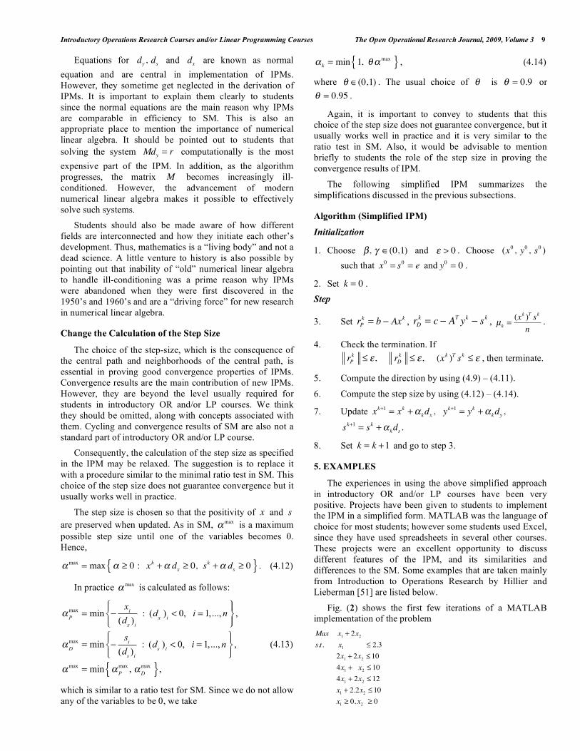
Fig. (2) shows the first few iterations of a MATLAB

implementation of the problem

Max x1 + 2x2s.t. x1 2.3

2x1 + 2x2 10

4x1 + x2 10

4x1 + 2x2 12

x1 + 2.2x2 10

x1 0, x2 0


Fig. (2).

Fig. (3) below shows first few iterations of the Excel

implementation of the above problem.

The “detour” in the path of iterations in the Fig. (2) is due

to matrix M becoming increasingly ill-conditioned, and not

surprisingly, Excel was less suitable to handle the problem

than MATLAB. This is also a good example to show what

problems may occur when we relax the calculation of the

step-size.

Fig. (3).

An important feature of the interior-point methods that

distinguish them from Simplex-type methods is that in the

case of infinitely many optimal solutions they converge to

the center of the optimal set rather than to the vertex. This is

illustrated in Fig. (4) below that shows a MATLAB

implementation of very simple example with infinitely many

optimal solutions.

Max 2x1 + 2x2s.t. x1 + x2 3

x1 0, x2 0

It is important to illustrate that the simplified version of

the IPM is an infeasible algorithm; that is, it is not required

that the method start from a point in the feasible region.

Fig. (5) below shows the first few iterations of a MATLAB

implementation of the problem

Fig. (4).

Max 3x1 + 5x2s.t. x1 4

2x2 12

3x1 + 2x2 18

x1 0, x2 0

with infeasible initial starting point.

Fig. (5).

Many other variations and modifications can be easily

discussed as well. Examples include how the change of

parameters influences the method, and how the change of

tolerance reflects on the number of iterations. In addition,

one interesting direction of modifying this basic simplified

version of IPM would be to incorporate Mehrota’s predictor-

corrector approach [60], which we briefly discussed at the

end of Section 3. The main idea is that two steps of the

Modified Newton’s Method be taken per iteration instead of

one. Then we can further compare these two approaches.


6. CONCLUSION

In this paper we have tried to show one way of

introducing IPMs for the introductory LP and/or OR courses

as well as other courses that contain LP as a part of their

content. The basic idea is to put the emphasis on the NM

while avoiding more advanced topics such as the Lagrange

functions, KKT conditions, barrier methods, and proofs of

convergence results. Several advantages of introducing IPMs

are listed below.

Often students in introductory OR and/or LP courses

think of Simplex-type methods as the only way to solve LP

problems. Introduction of IPMs shows that LP problems can

be solved using algorithms with quite a different approach

than the approach on which the SM was based. It also shows

students that their knowledge of calculus can be useful in a

place where they do not expect it. In addition, students

certainly benefit from seeing an important problem such as

the LP problem solved in two different ways. It opens

numerous possibilities for comparison of the two methods,

some of which were outlined in the previous sections.

With introduction of IPMs, the classical distinction

between linear programming methods, based on the SM and

methods of nonlinear programming, many of which are

based on NM, has largely disappeared. This opens up

possibilities for a more unifying approach to the large class

of optimization problems. In that sense, introduction of IPMs

into introductory OR and/or LP courses serves as a good

base for students who wish to proceed by studying Nonlinear

Programming and/or more advanced topics of IPMs.

Last, but not least, important is the fact that many, if not

the majority, of modern commercial and educational codes

for LP contain efficient IPM solvers. Computational

experiences in recent years have shown that they are often

more efficient than SM solvers, especially for large-scale

problems. Introducing IPMs will help students to better

understand and use these modern optimization codes.

REFERENCES

[1] Terlaky T. An easy way to teach interior point methods. Eur J Oper

Res 2001; 130(1): 1-19.

[2] Dantzig GB. Linear programming and extensions. Princeton NJ:

Princeton University Press 1963.

[3] Klee V, Minty GJ. How good is the simplex algorithm? In: Shisha

O, Ed. Inequalities. New York: Academic Press 1972; pp. 159-175.

[4] Murty KG. Computational complexity of complementary pivot

methods. Math Program Study 1978; 7: 61-73.

[5] Adler I, Megiddo N. A simplex algorithm whose average number

of steps is bounded between two quadratic functions of the smaller

dimension. J Assoc Comput Machinery 1985; 32: 891-95.

[6] Borgward KH. The Simplex method, a probabilistic analysis.

Bonn: Springer-Verlag 1987.

[7] Lesaja G. Complexity of linear programming problem. M.S. thesis,

University of Zagreb, Zagreb 1987.

[8] Smale S. On the average number of steps of the simplex method of

linear programming. Math Program 1983; 27: 241-62.

[9] Dobkin DR, Lipton R, Reiss S. Linear programming is P-complete:

Excursions in geometry. Report No. 71, Department of Computer

Science, Yale University 1976.

[10] Khachiyan LG. A polynomial algorithm in linear programming.

Sov Math Dokl 1979; 20: 191-94.

[11] Shor NZ. Cut-off method with space extensions in convex

programming. Kibernetika 1977; 6: 94-5.

[12] Grotshel M, Lovasz L, Shrijver A. The Ellipsoid method and

combinatorial optimization. Bonn: Springer-Verlag 1986.

[13] Bland R, Goldfarb D, Todd M. The ellipsoid method: a survey.

Oper Res 1981; 29(6): 1039-91.

[14] Karmarkar N. A polynomial-time algorithm for linear

programming. Combinatorica 1984; 4: 373-95.

[15] Kranich E. Interior-point methods for mathematical programming:

a bibliography. Discussionbeitrag 171, FerUniversitat Hagen,

Hagen, Germany 1991; (available through Netlib).

[16] Gill PE, Murray W, Saunders MA, Tomlin JA, Wright MH. On the

projected Newton barrier methods for linear programming and an

equivalence to Karmarkar’s projective method. Math Program

1986, 36: 183-209.

[17] Renegar J. A polynomial-time algorithm, based on Newton’s

method, for linear programming. Math Program 1988; 40: 59-73.

[18] Ye Y. An O(n3L) potential reduction algorithm for linear

programming. Math Program 1991; 50: 239-58.

[19] Kojima M, Mizuno S, Yoshise A. A primal-dual interior-point

algorithm for linear programming. In: Meggido N, Ed. Progress in

mathematical programming: Interior-point algorithms and related

methods, Berlin: Springer-Verlag 1989; pp. 29-47.

[20] Meggido N. Pathways to the optimal set in linear programming. In:

Meggido N, Ed. Progress in mathematical programming: interior-

point algorithms and related methods. Berlin: Springer-Verlag

1989; pp. 131-158.

[21] Sonnenvend G. An analytical center for polyhedrons and new

classes of global algorithms for linear (smooth, convex)

programming. In: Lecture notes in control and information sciences

84. Bonn: Springer-Verlag 1986, pp. 866-876.

[22] Anitescu M, Lesaja G, Potra F. An infeasible interior-point

predictor-corrector algorithm for the P*-geometric LCP. Appl Math

Optim 1997; 36: 203-28.

[23] Anitescu M, Lesaja G, Potra F. Equivalence between different

formulations of the linear complementarity problem. Optim

Methods Softw 1997; 7(3-4): 265-90.

[24] Kojima M, Megiddo N, Noma T, Yoshise A. A unified approach to

interior-point algorithms for linear complementarity problems.

Lecture Notes in Computer Science 538. Berlin: Springer-Verlag

1991.

[25] Kojima M, Mizuno S, Yoshise A. An O( nL) iteration potential-

reduction algorithm for linear complementarity problems. Math

Program 1991; 50: 331-42.

[26] Lesaja G. Interior-point methods for P*-complementarity problems.

Ph.D. thesis, University of Iowa, Iowa City 1996.

[27] Ye Y, Anstraicher K. On quadratic and O( nL) convergence of a

predictor-corrector algorithm for LCP. Math Program 1993; 62:

537-51.

[28] Roos C, Terlaky T, Vial J-PH. Interior-point approach to linear

optimization: Theory and algorithms 2nd ed. Berlin: Springer-

Verlag 2005.

[29] Andersen ED, Ye Y. On a homogeneous algorithm for the

monotone complementarity problem. Math Program 1999; 84(2):

375-99.

[30] Fachinei F, Pang J-S. Variational inequalities and complementarity

problems. Berlin: Springer-Verlag 2003; vol: I and II.

[31] Alizadeh F. Interior point methods in semidefinie programming

with applications to combinatorial optimization. SIAM J Optim

1995; 5: 13-51.

[32] Monteiro RDC. First- and second- order methods for semidefinite

programming. Math Program Series B 2003; 97(1-2): 209-44.

[33] Vandenberghe L, Boyd S. Semidefinite programming. SIAM Rev

1996; 38: 49-95.

[34] Ben-Tal A, Nemirovski A. Lectures on Modern Convex

Optimization: Analysis, Algorithms and Engineering Applications.

Philadelphia: SIAM Series on Optimization 2001.

[35] Nesterov YE, Nemirovski A. Interior-point polynomial methods in

convex programming. Philadelphia: SIAM Publications 1994.


[36] Terlaky T, Ed. Interior-point methods of mathematical

programming. Amsterdam: Kluwer 1996.

[37] Wright SJ. Primal-dual interior-point methods. Philadelphia: SIAM

Publications 1997.

[38] Ye Y. Interior-point algorithm: Theory and analysis. New York:

John Wiley 1997.

[39] Frisch KR. The logarithmic potential method of convex

programming. Technical Report, Institute of Economics, University

of Oslo, Norway 1955.

[40] Huard P. Resolution of mathematical programming with nonlinear

constraints by method of centers. In: Abadie J, Ed. Nonlinear

programming. Amsterdam: North Holland 1967.

[41] Barnes ER. A variation of Karmarkar’s algorithm for solving linear

programming problems. Math Program 1986; 36: 174-82.

[42] Vanderbei RJ, Meketon MS, Friedman BA. A modification of

Karmarkar’s linear programming algorithm. Algorithmica 1986;

1(4): 395-407.

[43] Dikin II. Iterative solution of problems of linear and quadratic

programming. Sov Math Dokl 1967; 8: 674-75.

[44] Fiacco AV, McCormick GP. Nonlinear programming: Sequential

unconstrained minimization technique. New York: Wiley 1968.

[45] Lootsma FA. Hessian matrices of penalty functions for solving

constrained optimization problems. Phil Res Rep 1969; 24: 322-31.

[46] Murray W. Analytical expressions for the eigenvalues and

eigenvectors of the Hessian matrices of barrier and penalty

functions. J Optim Theory Appl 1971; 7: 189-96.

[47] Anstreicher KM. On long step path following and SUMT for linear

programming. SIAM J Optim 1996; 6: 33-46.

[48] Andersen ED, Gondzio J, Meszaros C, Xu X. Implementation of

interior-point methods for large scale linear programming. In:

Terlaky T, Ed. Interior-point methods in mathematical

programming. Amsterdam: Kluwer 1996; pp. 217-245.

[49] Lustig IJ, Marsten RE, Shanno D. Interior-point methods for linear

programming: Computational state of the art. ORSA J Comput

1994; 6: 1-14.

[50] Mehrota S. On the implementation of a primal-dual interior-point

method. SIAM J Optim 1992; 2: 575-601.

[51] Hillier FS, Lieberman GJ. Introduction to operations research. 8th

ed. New York: McGraw Hill 2005.

[52] Goldman AJ, Tucker AW. Theory of linear programming. In: Kuhn

HW, Tucker AW, Eds. Linear equalities and related systems.

Princeton NJ: Princeton University Press 1956; pp. 53-97.

[53] Guler O, Ye Y. Convergence behavior of interior-point algorithms.

Math Program 1993; 60: 215-28.

[54] Mehrota S. Quadratic convergence in primal-dual methods. Math

Oper Res 1993; 18(3): 741-51.

[55] Yamashita H. A polynomially and quadratically convergent method

for linear programming. Research report, Mathematical Systems

Institute, Tokyo, Japan 1986.

[56] Ye Y, Guler O, Tapia RA, Zhang Y. A quadratically convergent

O( nL) - iteration algorithm for linear programming. Math

Program 1993; 59(2): 151-62.

[57] Ye Y, Todd MJ, Mizuno S. An O( nL) -iteration homogeneous

and self-dual linear programming algorithm. Math Oper Res 1994,

19: 208-27.

[58] Hung P, Ye Y. An asymptotical O( nL) -iteration path-following

linear programming algorithm that uses wide neighborhoods.

SIAM J Optim 1996; 6(3): 570-86.

[59] Ye Y. On the finite convergence of interior-point algorithms for

linear programming. Math Program 1992; 57: 325-36.

[60] Mehrota S. Higher order methods and their performance. Technical

Report, 90-16R1, Department of Industrial Engineering and

Management Sciences, Northwestern University, Evanston 1991.

[61] Bai YQ, Lesaja G, Roos C, Wang GQ, El Ghami M. A class of

large- and small-update primal-dual interior-point algorithms for

linear optimization. J Optim Theory Algorithms 2008; 138(3): 341-59.

[62] Peng J, Roos C, Terlaky T. Self-regularity: a new paradigm for

primal-dual interior-point algorithms. Princeton NJ: Princeton

University Press 2002.

Received: May 16, 2008 Revised: September 1, 2008 Accepted: May 6, 2009

© Goran Lesaja; Licensee Bentham Open.

This is an open access article licensed under the terms of the Creative Commons Attribution Non-Commercial License (http://creativecommons.org/licenses/by-nc/ 3.0/) which permits unrestricted, non-commercial use, distribution and reproduction in any medium, provided the work is properly cited.

Open Access Introducing Interior-Point Methods for ... · Introducing Interior-Point Methods for...

Documents

Transcript of Open Access Introducing Interior-Point Methods for ... · Introducing Interior-Point Methods for...