Online Learning in Case of Unbounded Losses Using Follow the

Journal of Machine Learning Research 12 (2011) 241-266 Submitted 8/10; Revised 12/10; Published 1/11

Online Learning in Case of Unbounded Losses Using Follow thePerturbed Leader Algorithm

Vladimir V. V’yugin VYUGIN @IITP.RU

Institute for Information Transmission ProblemsRussian Academy of SciencesBol’shoi Karetnyi per. 19Moscow GSP-4, 127994, Russia

Editor: Manfred Warmuth

AbstractIn this paper the sequential prediction problem with expertadvice is considered for the case wherelosses of experts suffered at each step cannot be bounded in advance. We present some modificationof Kalai and Vempala algorithm of following the perturbed leader where weights depend on pastlosses of the experts. New notions of a volume and a scaled fluctuation of a game are introduced.We present a probabilistic algorithm protected from unrestrictedly large one-step losses. This al-gorithm has the optimal performance in the case when the scaled fluctuations of one-step losses ofexperts of the pool tend to zero.

Keywords: prediction with expert advice, follow the perturbed leader, unbounded losses, adaptivelearning rate, expected bounds, Hannan consistency, online sequential prediction

1. Introduction

Experts algorithms are used for online prediction or repeated decision making or repeated gameplaying. Starting with the Weighted Majority Algorithm (WM) of Littlestone and Warmuth (1994)and Aggregating Algorithm of Vovk (1990), the theory of Prediction with Expert Advice has rapidlydeveloped in the recent times. Also, most authors have concentrated on predicting binary sequencesand have used specific (usually convex) loss functions, like absolute loss, square and logarithmicloss. A survey can be found in the book of Lugosi and Cesa-Bianchi (2006). Arbitrary lossesare less common, and, as a rule, they are supposed to be bounded in advance (see well knownHedge Algorithm of Freund and Schapire 1997, Normal Hedge of Chaudhuri et al. 2009 and otheralgorithms).

In this paper we consider a different general approach—“Follow the Perturbed Leader – FPL”algorithm, now called Hannan’s algorithm, see Hannan (1957), Kalai and Vempala (2003) and Lu-gosi and Cesa-Bianchi (2006). Under this approach we only choosethe decision that has fared thebest in the past—the leader. In order to cope with adversary some randomization is implementedby adding a perturbation to the total loss prior to selecting the leader. The goal of the learner’salgorithm is to perform almost as well as the best expert in hindsight in the long run. The resultingFPL algorithm has the same performance guarantees as WM-type algorithms for fixed learning rateand bounded one-step losses, save for a factor

√2. A major advantage of the FPL algorithm is that

its analysis remains easy for an adaptive learning rate, in contrast to WM-derivatives (see remarkin Hutter and Poland 2004).

c©2011 Vladimir V’yugin.

V’ YUGIN

Prediction with Expert Advice considered in this paper proceeds as follows. We are asked toperform sequential actions at timest = 1,2, . . . ,T. At each time stept, expertsi = 1, . . .N receiveresults of their actions in form of their lossessi

t—arbitrary real numbers.At the beginning of the stept Learner, observing cumulating lossessi

1:t−1 = si1+ . . .+ si

t−1 ofall expertsi = 1, . . .N, makes a decision to follow one of these experts, say Experti. At the end ofstept Learnerreceives the same losssi

t as Experti at stept and suffersLearner’scumulative losss1:t = s1:t−1+si

t .In the traditional framework, we suppose that one-step losses of all experts are bounded, for

example, 0≤ sit ≤ 1 for all i andt.

Well known simple example of a game with two experts shows that Learner can perform muchworse than each expert: let the current losses of two experts on stepst = 0,1, . . . ,6 bes1

0,1,2,3,4,5,6 =

(12,0,1,0,1,0,1) ands2

0.1,2,3,4,5,6 = (0,1,0,1,0,1,0). Evidently, “Follow the Leader” algorithm al-ways chooses the wrong prediction.

When the experts one-step losses are bounded, this problem has been solved using randomiza-tion of the experts cumulative losses. The method of following the perturbed leader was discoveredby Hannan (1957). Kalai and Vempala (2003) rediscovered this method and published a simpleproof of the main result of Hannan. They called an algorithm of this type FPL(Following thePerturbed Leader).

The FPL algorithm outputs prediction of an experti which minimizes

si1:t−1−

1ε

ξi ,

whereξi , i = 1, . . .N, t = 1,2, . . ., is a sequence of i.i.d random variables distributed according tothe exponential distribution with the densityp(x) = exp{−x}, andε is a learning rate.

Kalai and Vempala (2003) show that the expected cumulative loss of the FPLalgorithm has theupper bound

E(s1:t)≤ (1+ ε) mini=1,...,N

si1:t +

logNε

,

whereε is a positive real number such that 0< ε < 1 is a learning rate,N is the number of experts.Hutter and Poland (2004, 2005) presented a further developments of theFPL algorithm for

countable class of experts, arbitrary weights and adaptive learning rate. Also, FPL algorithm isusually considered for bounded one-step losses: 0≤ si

t ≤ 1 for all i andt. Using a variable learningrate, an optimal upper bound was obtained in Hutter and Poland (2005):

E(s1:t)≤ mini=1,...,N

si1:t +2

√2T lnN.

Most papers on prediction with expert advice either consider bounded losses or assume the existenceof a specific loss function (see Lugosi and Cesa-Bianchi 2006). We allow losses at any step to beunbounded. The notion of a specific loss function is not used.

The setting allowing unbounded one-step losses do not have wide coverage in literature; wecan only refer reader to Allenberg et al. (2006), Cesa-Bianchi et al.(2007) and Poland and Hutter(2005).

Poland and Hutter (2005) have studied the games where one-step losses of all experts at eachstept are bounded from above by an increasing sequenceBt given in advance. They presented alearning algorithm which is asymptotically consistent forBt = t1/16.

242

LEARNING IN CASE OFUNBOUNDED LOSSESUSING FPL ALGORITHM

Allenberg et al. (2006) have considered polynomially bounded one-steplosses for a modifiedversion of the Littlestone and Warmuth (1994) algorithm under partial monitoring. In full infor-mation case, their algorithm has the expected regret 2

√N lnN(T + 1)

12(1+a+β) in the case where

one-step losses of all expertsi = 1,2, . . .N at each stept have the bound(sit)

2 ≤ ta, wherea> 0, andβ > 0 is a parameter of the algorithm. They have proved that this algorithm is Hannan consistent if

max1≤i≤N

1T

T

∑t=1

(sit)

2 < cTa

for all T, wherec> 0 and 0< a< 1.Cesa-Bianchi et al. (2007) derived a new forecasting strategy for the Weighted Majority algo-

rithm in unbounded setting with regret√

QT lnN+MT lnN,

whereMT = max1≤i≤N max1≤t≤T |sit | is the largest absolute value of any losssi

t of an experti at

time stepT, andQT =T∑

t=1(simin

t )2 is the sum of squared losses of the best at firstT steps expertimin.

These bounds were improved using cumulative variances of losses (under distributions used in theWeighted Majority algorithm). Cesa-Bianchi et al. (2007) do not study asymptotic consistency oftheir algorithm.

In this paper we present a sufficient condition for the FPL algorithm to be asymptotically con-sistent in case where losses are unbounded. In particular, this setting covers a case where loss grows“faster than polynomial, but slower than exponential”. We present some modification of Kalai andVempala (2003) algorithm of following the perturbed leader (FPL) for the case of unrestrictedlylarge one-step expert lossessi

t not bounded in advance:sit ∈ (−∞,+∞). This algorithm uses adap-

tive weights depending on past cumulative losses of the experts.A motivating example, where losses of the experts cannot be bounded in advance, is given in

Section 5.The full information case is considered in this paper. We analyze the asymptotic consistency

of our algorithms using nonstandard scaling. We introduce new notions ofthe volume of a game

vt = v0+t∑j=1

maxi |sij | andthe scaled fluctuationof the game fluc(t) = ∆vt/vt , where∆vt = vt −vt−1

andv0 is a nonnegative constant.We show in Theorem 2 that the algorithm of following the perturbed leader withadaptive

weights constructed in Section 3 is asymptotically consistent in the mean in the casewherevt → ∞and∆vt = o(vt) ast → ∞ with a computable bound. Specifically, if fluc(t) ≤ γ(t) for all t, whereγ(t) is a computable function such thatγ(t) = o(1) ast → ∞, our algorithm has the expected regret

2√

(8+ ε)(1+ lnN)T

∑t=1

(γ(t))1/2∆vt ,

whereε > 0 is a parameter of the algorithm.In case where all losses are nonnegative:si

t ∈ [0,+∞), we obtain the regret

2√

(2+ ε)(1+ lnN)T

∑t=1

(γ(t))1/2∆vt .

243

V’ YUGIN

In particular, this algorithm is asymptotically consistent (in the mean) in a modified sense

limsupT→∞

1vT

E(s1:T − mini=1,...N

si1:T)≤ 0, (1)

wheres1:T is the total loss of our algorithm on steps 1,2, . . .T, andE(s1:T) is its expectation.Proposition 1 of Section 2 shows that if the condition∆vt = o(vt) is violated the cumulative loss

of any probabilistic prediction algorithm can be much more than the loss of the best expert of thepool.

In Section 3 we present some sufficient conditions under which our learning algorithm is Hannanconsistent.1

In Section 4 we consider some special cases of our algorithm and applications for the case ofstandard time-scaling.

In particular, Corollary 8 of Theorem 2 says that our algorithm is asymptotically consistent (inthe modified sense) in the case when one-step losses of all experts at each stept are bounded byta,wherea is a positive real number. We prove this result under an extra assumption that the volumeof the game grows slowly, liminf

t→∞vt/ta+δ > 0, whereδ > 0 is arbitrary. Corollary 8 shows that our

algorithm is also Hannan consistent whenδ > 12.

In Section 5 we consider an application of our algorithm for constructing anarbitrage strategyin some game of buying and selling shares of some stock on financial market. We analyze this gamein the decision theoretic online learning (DTOL) framework (see Freund and Schapire 1997). WeintroduceLearnerthat computes weighted average of different strategies with unbounded gains andlosses. To change from the follow leader framework to DTOL we derandomize our FPL algorithm.

This paper is an extended version of the ALT 2009 conference paper V’yugin (2009).

2. Games of Prediction with Expert Advice with Unbounded One-step Losses

We consider a game of prediction with expert advice with arbitrary unbounded one-step losses.Following Cesa-Bianchi et al. (2007) we call a game with such losses “signed game” and call theselosses “signed losses”.

At each stept of the game, allN experts receive one-step lossessit ∈ (−∞,+∞), i = 1, . . .N, and

the cumulative loss of theith expert after stept is equal to

si1:t = si

1:t−1+sit .

A probabilistic learning algorithm of choosing an expert outputs at any stept the probabilitiesP{It = i} of following the ith expert given the cumulative lossessi

1:t−1 of the expertsi = 1, . . .N inhindsight (see Figure 1).

The performance of this probabilistic algorithm is measured in itsexpected regret


si1:T),

where the random variables1:T is the cumulative loss of the master algorithm,si1:T , i = 1, . . .N, are

the cumulative losses of the experts algorithms andE is the mathematical expectation (with respect

1. This means that (1) holds with probability 1, whereE is omitted.

244


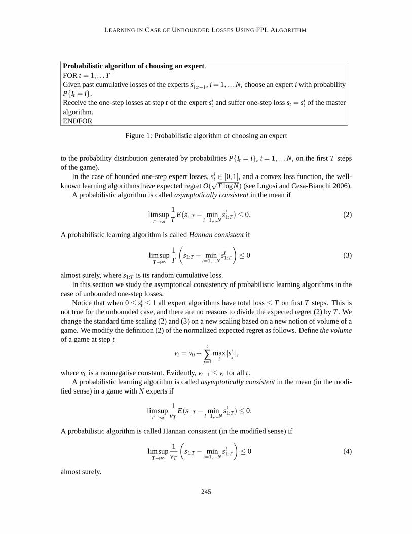
Probabilistic algorithm of choosing an expert.FORt = 1, . . .TGiven past cumulative losses of the expertssi

1:t−1, i = 1, . . .N, choose an experti with probabilityP{It = i}.Receive the one-step losses at stept of the expertsi

t and suffer one-step lossst = sit of the master

algorithm.ENDFOR

Figure 1: Probabilistic algorithm of choosing an expert

to the probability distribution generated by probabilitiesP{It = i}, i = 1, . . .N, on the firstT stepsof the game).

In the case of bounded one-step expert losses,sit ∈ [0,1], and a convex loss function, the well-

known learning algorithms have expected regretO(√

T logN) (see Lugosi and Cesa-Bianchi 2006).A probabilistic algorithm is calledasymptotically consistentin the mean if

limsupT→∞

1T


si1:T)≤ 0. (2)

A probabilistic learning algorithm is calledHannan consistentif

limsupT→∞

1T

(

s1:T − mini=1,...N

si1:T

)

≤ 0 (3)

almost surely, wheres1:T is its random cumulative loss.In this section we study the asymptotical consistency of probabilistic learning algorithms in the

case of unbounded one-step losses.Notice that when 0≤ si

t ≤ 1 all expert algorithms have total loss≤ T on firstT steps. This isnot true for the unbounded case, and there are no reasons to divide the expected regret (2) byT. Wechange the standard time scaling (2) and (3) on a new scaling based on a new notion of volume of agame. We modify the definition (2) of the normalized expected regret as follows. Definethe volumeof a game at stept

vt = v0+t

∑j=1

maxi

|sij |,

wherev0 is a nonnegative constant. Evidently,vt−1 ≤ vt for all t.A probabilistic learning algorithm is calledasymptotically consistentin the mean (in the modi-

fied sense) in a game withN experts if

limsupT→∞

1vT


si1:T)≤ 0.

A probabilistic algorithm is called Hannan consistent (in the modified sense) if

limsupT→∞

1vT

(

s1:T − mini=1,...N

si1:T

)

≤ 0 (4)

almost surely.

245

V’ YUGIN

Notice that the notions of asymptotic consistency in the mean and Hannan consistency may benon-equivalent for unbounded one-step losses.

A game is callednon-degenerateif vt → ∞ ast → ∞.Denote∆vt = vt −vt−1. The number

fluc(t) =∆vt

vt=

maxi |sit |

vt,

is calledscaled fluctuationof the game at the stept.By definition 0≤ fluc(t)≤ 1 for all t (put 0/0= 0).The following simple proposition shows that each probabilistic learning algorithm is not asymp-

totically optimal in some game such that fluc(t) 6→ 0 ast → ∞. For simplicity, we consider the caseof two experts and nonnegative losses.

Proposition 1 For any probabilistic algorithm of choosing an expert and for anyε such that0 <ε < 1 two experts exist such that vt → ∞ as t→ ∞ and

fluc(t)≥ 1− ε,1vt

E(s1:t − mini=1,2

si1:t)≥

12(1− ε)

for all t.

Proof. Given a probabilistic algorithm of choosing an expert andε such that 0< ε < 1, definerecursively one-step lossess1

t ands2t of expert 1 and expert 2 at any stept = 1,2, . . . as follows.

By s11:t ands2

1:t denote the cumulative losses of these experts incurred at steps≤ t, let vt be thecorresponding volume, wheret = 1,2, . . ..

Definev0 = 1 andMt = 4vt−1/ε for all t ≥ 1. For t ≥ 1, defines1t = Mt ands2

t = 0 if P{It =1} ≥ 1

2, and defines1t = 0 ands2

t = Mt otherwise.Let st be one-step loss of the master algorithm ands1:t be its cumulative loss at stept ≥ 1. We

have

E(s1:t)≥ E(st) = s1t P{It = 1}+s2

t P{It = 2} ≥ 12

Mt

for all t ≥ 1. Also, sincevt = vt−1+Mt = (1+4/ε)vt−1 and mini

si1:t ≤ vt−1, the normalized expected

regret of the master algorithm is bounded from below

1vt

E(s1:t −mini

si1:t)≥

2/ε−11+4/ε

≥ 12(1− ε).

for all t. By definition

fluc(t) =Mt

vt−1+Mt=

11+ ε/4

≥ 1− ε

for all t. △Proposition 1 shows that we should impose some restrictions of asymptotic behavior of fluc(t)

to prove the asymptotic consistency of a probabilistic algorithm.

246


3. Follow the Perturbed Leader Algorithm with Adaptive Weights

In this section we construct the FPL algorithm with adaptive weights protectedfrom unboundedone-step losses.

Let γ(t) be a computable non-increasing real function such that 0< γ(t) < 1 for all t. In thatfollows we usually assumeγ(t) → 0 ast → ∞; for example,γ(t) = 1/(t + c)δ, wherec > 0 andδ > 0. Let alsoa be a positive real number. Define

αt =12

1−ln a(1+lnN)

2(e4/a−1)

lnγ(t)

and (5)

µt = a(γ(t))αt =

√

2a(e4/a−1)(1+ lnN)

(γ(t))1/2 (6)

for all t, wheree= 2.72. . . is the base of the natural logarithm.2

Without loss of generality we suppose thatγ(t)< min{A,A−1} for all t, where

A=2(e4/a−1)a(1+ lnN)

.

We can obtain this choosing an appropriate value of the initial constantv0. Then 0< αt < 1 for allt.

We consider an FPL algorithm with a variable learning rate

εt =1

µtvt−1, (7)

whereµt is defined by (6) and the volumevt−1 depends on experts actions on steps< t. By definitionvt ≥ vt−1 andµt ≤ µt−1 for t = 1,2, . . .. Also, by definitionµt → 0 ast → ∞ if γ(t)→ 0.

Let ξ1t ,. . .ξN

t , t = 1,2, . . ., be a sequence of i.i.d random variables distributed exponentially withthe densityp(x) = exp{−x}. In what follows we omit the lower indext.

We suppose without loss of generality thatsi0 = v0 = 0 for all i andε0 = ∞.

The FPL algorithm PROT is defined on Figure 2.

Let s1:T =T∑

t=1sItt be the cumulative loss of the FPL algorithm on steps≤ T.

The following theorem shows that if the game is non-degenerate and∆vt = o(vt) as t → ∞with a computable bound then the FPL-algorithm with variable learning rate (7) isasymptoticallyconsistent.

We suppose that the experts are oblivious, that is, they do not use in theirwork random actionsof the learning algorithm. The inequality (9) of Theorem 2 below is reformulatedand proved fornon-oblivious experts at the end this section.

Theorem 2 Assume that a computable non-increasing real functionγ(t) exists such that0< γ(t)<1 and

fluc(t)≤ γ(t) (8)

2. The choice of the optimal value ofαt will be explained later. It will be obtained by minimization of the correspondingmember of the sum (36).

247

V’ YUGIN

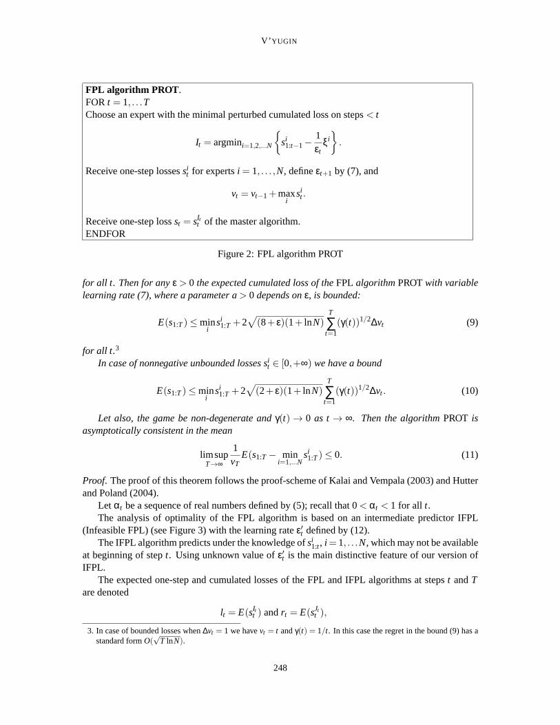
FPL algorithm PROT .FORt = 1, . . .TChoose an expert with the minimal perturbed cumulated loss on steps< t

It = argmini=1,2,...N

{

si1:t−1−

1εt

ξi}

.

Receive one-step lossessit for expertsi = 1, . . . ,N, defineεt+1 by (7), and

vt = vt−1+maxi

sit .

Receive one-step lossst = sItt of the master algorithm.

ENDFOR

Figure 2: FPL algorithm PROT

for all t. Then for anyε > 0 the expected cumulated loss of theFPL algorithmPROTwith variablelearning rate (7), where a parameter a> 0 depends onε, is bounded:

E(s1:T)≤ mini

si1:T +2

√

(8+ ε)(1+ lnN)T

∑t=1

(γ(t))1/2∆vt (9)

for all t.3

In case of nonnegative unbounded losses sit ∈ [0,+∞) we have a bound

E(s1:T)≤ mini

si1:T +2

√

(2+ ε)(1+ lnN)T

∑t=1

(γ(t))1/2∆vt . (10)

Let also, the game be non-degenerate andγ(t) → 0 as t→ ∞. Then the algorithmPROT isasymptotically consistent in the mean

limsupT→∞

1vT


si1:T)≤ 0. (11)

Proof. The proof of this theorem follows the proof-scheme of Kalai and Vempala(2003) and Hutterand Poland (2004).

Let αt be a sequence of real numbers defined by (5); recall that 0< αt < 1 for all t.The analysis of optimality of the FPL algorithm is based on an intermediate predictor IFPL

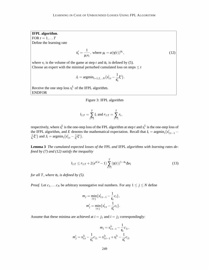
(Infeasible FPL) (see Figure 3) with the learning rateε′t defined by (12).The IFPL algorithm predicts under the knowledge ofsi

1:t , i = 1, . . .N, which may not be availableat beginning of stept. Using unknown value ofε′t is the main distinctive feature of our version ofIFPL.

The expected one-step and cumulated losses of the FPL and IFPL algorithmsat stepst andTare denoted

lt = E(sItt ) andrt = E(sJt

t ),

3. In case of bounded losses when∆vt = 1 we havevt = t andγ(t) = 1/t. In this case the regret in the bound (9) has astandard formO(

√T lnN).

248


IFPL algorithm .FORt = 1, . . .TDefine the learning rate

ε′t =1

µtvt, whereµt = a(γ(t))αt , (12)

wherevt is the volume of the game at stept andαt is defined by (5).Choose an expert with the minimal perturbed cumulated loss on steps≤ t

Jt = argmini=1,2,...N{si1:t −

1ε′t

ξi}.

Receive the one step losssJtt of the IFPL algorithm.

ENDFOR

Figure 3: IFPL algorithm

l1:T =T

∑t=1

lt andr1:T =T

∑t=1

rt ,

respectively, wheresItt is the one-step loss of the FPL algorithm at stept andsJt

t is the one-step loss ofthe IFPL algorithm, andE denotes the mathematical expectation. Recall thatIt = argmini{si

1:t−1−1εt

ξi} andJt = argmini{si1:t − 1

ε′tξi}.

Lemma 3 The cumulated expected losses of theFPL and IFPL algorithms with learning rates de-fined by (7) and (12) satisfy the inequality

l1:T ≤ r1:T +2(e4/a−1)T

∑t=1

(γ(t))1−αt ∆vt (13)

for all T , whereαt is defined by (5).

Proof. Let c1, . . .cN be arbitrary nonnegative real numbers. For any 1≤ j ≤ N define

mj = mini 6= j

{si1:t−1−

1εt

ci},

m′j = min

i 6= j{si

1:t −1ε′t

ci}.

Assume that these minima are achieved ati = j1 andi = j2 correspondingly:

mj = sj11:t−1−

1εt

c j1,

m′j = sj2

1:t −1ε′t

c j2 = sj21:t−1+sj2

t − 1ε′t

c j2

249

V’ YUGIN

for somej1 and j2. By definition j1 6= j and j2 6= j. Then we have

mj = sj11:t−1−

1εt

c j1 ≤ sj21:t−1−

1εt

c j2 ≤

≤ sj21:t−1+sj2

t +∆vt −1εt

c j2 = (14)

= sj21:t +∆vt −

1ε′t

c j2 +

(

1ε′t− 1

εt

)

c j2 =

= m′j +∆vt +

(

1ε′t− 1

εt

)

c j2. (15)

We add∆vt to the right-hand side of the inequality (14) since the termsj2t may be negative in case

of signed losses. In case of nonnegative losses we need not to do this.Comparing conditional probabilities

P{It = j|ξi = ci , i 6= j} andP{Jt = j|ξi = ci i 6= j}

is the core of the proof of the lemma.The following chain of equalities and inequalities is valid:

P{It = j|ξi = ci , i 6= j}=

= P{sj1:t−1−

1εt

ξ j ≤ mj |ξi = ci , i 6= j}=

= P{ξ j ≥ εt(sj1:t−1−mj)|ξi = ci , i 6= j}=

= P{ξ j ≥ ε′t(sj1:t−1−mj)+(εt − ε′t)(s

j1:t−1−mj)|ξi = ci , i 6= j} ≤ (16)

≤ P{ξ j ≥ ε′t(sj1:t−1−mj)+

+(εt − ε′t)(sj1:t−1−sj2

1:t−1+1εt

c j2)|ξi = ci , i 6= j}= (17)

= P{ξ j ≥ ε′t(sj1:t−1−mj)+

+(εt − ε′t)(sj1:t−1−sj2

1:t−1)+(εt − ε′t)1εt

c j2|ξi = ci , i 6= j} ≤ (18)

≤ P{ξ j ≥ ε′t(sj1:t −sj

t −m′j −∆vt −

(

1ε′t− 1

εt

)

c j2)+

+(εt − ε′t)(sj1:t−1−sj2

1:t−1)+(εt − ε′t)1εt

c j2|ξi = ci , i 6= j}= (19)

= P{ξ j ≥ ε′t(sj1:t −m′

j)+

+(εt − ε′t)(sj1:t−1−sj2

1:t−1)− ε′t(sjt +∆vt)|ξi = ci , i 6= j}=

= P{ξ j >1

µtvt(sj

1:t −m′j)+

+

(

1µtvt−1

− 1µtvt

)

(sj1:t−1−sj2

1:t−1)−sjt +∆vt

µtvt|ξi = ci , i 6= j} ≤ (20)

≤ P{ξ j >1

µtvt(sj

1:t −m′j)+

250


+∆vt

µtvt

(sj1:t−1−sj2

1:t−1)

vt−1− 2∆vt

µtvt|ξi = ci , i 6= j} ≤ (21)

≤ exp

{

∆vt

µtvt

∣

∣

∣

∣

∣

sj1:t−1−sj2

1:t−1

vt−1−2

∣

∣

∣

∣

∣

}

× (22)

×P{Jt = j|ξi = ci , i 6= j}. (23)

Here the inequality (16)–(17) follows from (14) andεt ≥ ε′t . The inequality (18–(19) follows from(15). We have used in transition from (20) to (21) the equalityvt − vt−1 = ∆vt and the inequality|sj

t | ≤ ∆vt for all j andt. We have used in transition from (21) to (22)–(23) the inequalityP{ξ ≥a+b} ≤ e|b|P{ξ ≥ a} for any random variableξ distributed according to the exponential law, wherea andb are arbitrary real numbers.4

We have in (22)∣

∣

∣

∣

∣

sj1:t−1−sj2

1:t−1

vt−1

∣

∣

∣

∣

∣

≤ 2, (24)

since∣

∣

∣

si1:t−1vt−1

∣

∣

∣≤ 1 for all t andi. Also, ∆vt/vt ≤ γ(t) andµt = a(γ(t))αt . Therefore, we obtain

P{It = j|ξi = ci , i 6= j} ≤

≤ exp

{

4µt

∆vt

vt

}

P{Jt = j|ξi = ci , i 6= j} ≤

≤ exp{(4/a)(γ(t))1−αt}P{Jt = j|ξi = ci , i 6= j}. (25)

Since, the inequality (25) holds for allci , it also holds unconditionally :

P{It = j} ≤ exp{(4/a)(γ(t))1−αt}P{Jt = j}. (26)

for all t = 1,2, . . . and j = 1, . . .N.Sincesj

t +∆vt ≥ 0 for all j andt, we obtain from (26)

lt +∆vt = E(sItt +∆vt) =

N

∑j=1

(sjt +∆vt)P(It = j)≤

≤ exp{(4/a)(γ(t))1−αt}N

∑j=1

(sjt +∆vt)P(Jt = j) =

= exp{(4/a)(γ(t))1−αt}(E(sJtt )+∆vt) =

= exp{(4/a)(γ(t))1−αt}(rt +∆vt)≤≤ (1+(e4/a−1))(γ(t))1−αt )(rt +∆vt) =

= rt +∆vt +(e4/a−1)(γ(t))1−αt (rt +∆vt)≤≤ rt +∆vt +2(e4/a−1)(γ(t))1−αt ∆vt . (27)

4. Fora ≤ 0, we haveP{ξ ≥ a+b} ≤ e|b|P{ξ ≥ a} for all b, sinceP{ξ ≥ a} = 1 andP{ξ ≥ a+b} ≤ 1; for a > 0,P{ξ ≥ a+b} ≤ e−bP{ξ ≥ a} for all b.

251

V’ YUGIN

In the last line of (27) we have used the inequality|rt | ≤ ∆vt for all t and the inequalityesr ≤1+(es−1)r for all 0≤ r ≤ 1 ands> 0.

Subtracting∆vt from both sides of the inequality (27) and summing it byt = 1, . . .T, we obtain

l1:T ≤ r1:T +2(e4/a−1)T

∑t=1

(γ(t))1−αt ∆vt

for all T. Lemma 3 is proved.△The following lemma, which is an analogue of the result of Kalai and Vempala (2003), gives a

bound for the IFPL algorithm.

Lemma 4 The expected cumulative loss of theIFPLalgorithm with the learning rate (12) is bounded :

r1:T ≤ mini

si1:T +a(1+ lnN)

T

∑t=1

(γ(t))αt ∆vt (28)

for all T , whereαt is defined by (5).

Proof. The proof is along the line of the proof of Hutter and Poland (2004) with anexception thatnow the sequenceε′t is not monotonic.

Let in this proof,st = (s1t , . . .s

Nt ) be a vector of one-step losses ands1:t = (s1

1:t , . . .sN1:t) be a

vector of cumulative losses of the experts algorithms. Also, letξ = (ξ1, . . .ξN) be a vector whosecoordinates are random variables.

Recall thatε′t = 1/(µtvt), µt ≤ µt−1 for all t, andv0 = 0, ε′0 = ∞.

Defines̃1:t = s1:t− 1ε′t

ξ for t = 1,2, . . .. Consider the vector of one-step lossess̃t = st−ξ(

1ε′t− 1

ε′t−1

)

for the moment.For any vectors and a unit vectord denote

M(s) = argmind∈D{d ·s},

whereD = {(0, . . .1), . . . ,(1, . . .0)} is the set of N unit vectors of dimension N and “·” is the innerproduct of two vectors.

We first show that

T

∑t=1

M(s̃1:t) · s̃t ≤ M(s̃1:T) · ˜s1:T . (29)

ForT = 1 this is obvious. For the induction step fromT −1 toT we need to show that

M(s̃1:T) · s̃T ≤ M(s̃1:T) · s̃1:T −M(s̃1:T−1) · s̃1:T−1.

This follows froms̃1:T = s̃1:T−1+ s̃T and

M(s̃1:T) · s̃1:T−1 ≥ M(s̃1:T−1) · s̃1:T−1.

We rewrite (29) as follows

T

∑t=1

M(s̃1:t) ·st ≤ M(s̃1:T) · s̃1:T +T

∑t=1

M(s̃1:t) ·ξ(

1ε′t− 1

ε′t−1

)

. (30)

252


By definition ofM we have

M(s̃1:T) · s̃1:T ≤ M(s1:T) ·(

s1:T −ξε′T

)

=

= mind∈D

{d ·s1:T}−M(s1:T) ·ξε′T

. (31)

The expectation of the last term in (31) is equal to1ε′T

= µTvT .The second term of (30) can be rewritten

T

∑t=1

M(s̃1:t) ·ξ(

1ε′t− 1

ε′t−1

)

=

=T

∑t=1

(µtvt −µt−1vt−1)M(s̃1:t) ·ξ . (32)

We will use the standard inequality for the mathematical expectationE

0≤ E(M(s̃1:t) ·ξ)≤ E(maxi

ξi)≤ 1+ lnN. (33)

The proof of this inequality uses ideas from Kalai and Vempala (2003) andHutter and Poland (2004)(Lemma 1).

We have for the exponentially distributed random variablesξi , i = 1, . . .N,

P{maxi

ξi ≥ a}= P{∃i(ξi ≥ a)} ≤N

∑i=1

P{ξi ≥ a}= Nexp{−a}. (34)

Since for any non-negative random variableη, E(η) =∞∫0

P{η ≥ y}dy, by (34) we have

E(maxi

ξi − lnN) =

=

∞∫

0

P{maxi

ξi − lnN ≥ y}dy≤

≤∞∫

0

Nexp{−y− lnN}dy= 1.

Therefore,E(maxi ξi)≤ 1+ lnN.By (33) the expectation of (32) has the upper bound

T

∑t=1

E(M(s̃1:t) ·ξ)(µtvt −µt−1vt−1)≤ (1+ lnN)T

∑t=1

µt∆vt .

Here we have used the inequalityµt ≤ µt−1 for all t,SinceE(ξi) = 1 for all i, the expectation of the last term in (31) is equal to

E

(

M(s1:T) ·ξε′T

)

=1ε′T

= µTvT . (35)

253

V’ YUGIN

Combining the bounds (30)-(32) and (35), we obtain

r1:T = E

(

T

∑t=1

M(s̃1:t) ·st

)

≤

≤ mini

si1:T −µTvT +(1+ lnN)

T

∑t=1

µt∆vt ≤

≤ mini

si1:T +(1+ lnN)

T

∑t=1

µt∆vt .

Lemma is proved.△.We finish now the proof of the theorem.The inequality (13) of Lemma 3 and the inequality (28) of Lemma 4 imply the inequality

E(s1:T)≤ mini

si1:T +

+T

∑t=1

(2(e4/a−1)(γ(t))1−αt +a(1+ lnN)(γ(t))αt )∆vt . (36)

for all T.The optimal value (5) ofαt can be easily obtained by minimization of each member of the sum

(36) byαt . In this caseµt is equal to (6) and (36) is equivalent to

E(s1:T)≤ mini

si1:T +2

√

2a(e4/a−1)(1+ lnN)T

∑t=1

(γ(t))1/2∆vt , (37)

wherea is a parameter of the algorithm PROT.Also, for eachε > 0 ana exists such that 2a(e4/a−1)< 8+ ε. Therefore, we obtain (9).We have∑T

t=1 ∆vt = vT for all T, vt → ∞ andγ(t)→ 0 ast → ∞. Then by Toeplitz lemma (seeLemma 9 of Section A)

1vT

(

2√

(8+ ε)(1+ lnN)T

∑t=1

(γ(t))1/2∆vt

)

→ 0

asT → ∞. Therefore, the FPL algorithm PROT is asymptotically consistent in the mean, that is, therelation (11) of Theorem 2 is proved.

In case where all losses are nonnegative:sit ∈ [0,+∞), the inequality (24) can be replaced on

∣

∣

∣

∣

∣

sj1:t−1−sj2

1:t−1

vt−1

∣

∣

∣

∣

∣

≤ 1

for all t andi. We need not to add the term∆vt to the right-hand side of the inequality (14). Also,we need not to add∆vt to both parts of inequality (27).

In this case an analysis of the proof of Lemma 3 shows that the bound (37) can be replaced on

E(s1:T)≤ mini

si1:T +2

√

a(e2/a−1)(1+ lnN)T

∑t=1

(γ(t))1/2∆vt ,

254


wherea is a parameter of the algorithm PROT.For eachε > 0 ana exists such thata(e2/a−1) < 2+ ε. Using this parametera, we obtain a

version of (9) for nonnegative losses—the inequality (10).△We study now the Hannan consistency of our algorithm.

Theorem 5 Assume that all conditions of Theorem 2 hold and

∞

∑t=1

(γ(t))2 < ∞. (38)

Then the algorithmPROTis Hannan consistent:

limsupT→∞

1vT

(

s1:T − mini=1,...N

si1:T

)

≤ 0 (39)

almost surely.

Proof. So far we assumed that perturbationsξ1, . . . ,ξN are sampled only once at timet = 0. Thischoice was favorable for the analysis. As it easily seen, under expectation this is equivalent to gen-erating new perturbationsξ1

t , . . . ,ξNt at each time stept; also, we assume that all these perturbations

are i.i.d for i = 1, . . . ,N andt = 1,2, . . .. Lemmas 3, 4 and Theorem 2 remain valid for this case.This method of perturbation is needed to prove the Hannan consistency of the algorithm PROT.

We use some version of the strong law of large numbers to prove the Hannanconsistency of thealgorithm PROT.

Proposition 6 Let g(x) be a positive nondecreasing real function such that x/g(x), g(x)/x2 arenon-increasing for x> 0 and g(x) = g(−x) for all x.

Let the assumptions of Theorem 2 hold and

∞

∑t=1

g(∆vt)

g(vt)< ∞. (40)

Then theFPL algorithmPROTis Hannan consistent, that is, (4) holds as T→ ∞ almost surely.

Proof. The proof is based on the following lemma.

Lemma 7 Let at be a nondecreasing sequence of real numbers such that at → ∞ as t→ ∞ and Xt

be a sequence of independent random variables such that E(Xt) = 0, for t = 1,2, . . .. Let also, g(x)satisfies assumptions of Proposition 6. Then the inequality

∞

∑t=1

E(g(Xt))

g(at)< ∞ (41)

implies

1aT

T

∑t=1

Xt → 0 (42)

as T→ ∞ almost surely.

255

V’ YUGIN

The proof of this lemma is given in Section A.PutXt = (st −E(st))/2, wherest is the loss of the FPL algorithm PROT at stept, andat = vt for

all t. By definition|Xt | ≤ ∆vt for all t. Then (41) is valid, and by (42)

1vT

(s1:T −E(s1:T)) =1vT

T

∑t=1

(st −E(st))→ 0

asT → ∞ almost surely. This limit and the limit (11) imply (39).△By Lemma 6 the algorithm PROT is Hannan consistent, since (38) implies (40) forg(x) = x2.

Theorem 5 is proved.△Non-asymptotic version of Theorem 5 can be obtained but this requires more heavy technics

from probability theory (see Petrov 1975).

4. Specializations of Theorems 2 and 5

In this section we discuss some special cases of Theorems 2 and 5.In case of bounded experts lossessi

t ∈ [0,1], assume that an auxiliary “bad” experti0 existsfor which si0

t = 1 for all t. Then∆vt = 1 and the volume becomes time:vt = t for all t (we putv0 = 0). So, we can takeγ(t) = t−1 for all t. In this case the regret (10) of Theorem 2 is equal to4√

(2+ ε)(1+ lnN)T that is very close to classical bounds from Hutter and Poland (2004), Kalaiand Vempala (2003) and Lugosi and Cesa-Bianchi (2006).

Allenberg et al. (2006) and Poland and Hutter (2005) considered polynomially bounded one-step losses. We consider a specific example of the bound (9) for polynomial case.

Corollary 8 Assume that|sit | ≤ tα for all t and i= 1, . . .N, and vt ≥ tα+δ for all t, whereα andδ

are positive real numbers. Let also, in the algorithmPROT, γ(t) = t−δ and µt is defined by (6). Then

• (i) the algorithmPROTis asymptotically consistent in the mean for anyα > 0 andδ > 0;

• (ii) this algorithm is Hannan consistent for anyα > 0 andδ > 12;

• (iii) the expected loss of this algorithm is bounded :

E(s1:T)≤ mini

si1:T +2

√

(8+ ε)(1+ lnN)T1− 12δ+α (43)

as T→ ∞, whereε > 0 is a parameter of the algorithm.5

This corollary follows directly from Theorem 2, where condition (38) of Theorem 2 holds forδ > 12.

If δ = 1 the regret from (43) is asymptotically equivalent to the regret from Allenberg et al.(2006) (see Section 1).

Forα = 0 we have the case of bounded loss function (|sit | ≤ 1 for all i andt). The FPL algorithm

PROT is asymptotically consistent in the mean ifvt ≥ β(t) for all t, whereβ(t) is an arbitrarypositive unbounded non-decreasing computable function (we can getγ(t) = 1/β(t) in this case).This algorithm is Hannan consistent if (38) holds, that is,

∞

∑t=1

(β(t))−2 < ∞.

5. Recall that givenε we tune the parametera of the algorithm PROT.

256


For example, this condition be satisfied forβ(t) = t1/2 ln t.Let us show that the bound (9) of Theorem 2 that holds against oblivious experts also holds

against non-oblivious (adaptive) ones.In non-oblivious case, it is natural to generate at each time stept of the algorithm PROT a

new vector of perturbations̄ξt = (ξ1t , . . . ,ξN

t ), ξ̄0 is empty set. Also, it is assumed that all theseperturbations are i.i.d according to the exponential distributionP, wherei = 1, . . . ,N andt = 1,2, . . ..Denoteξ̄1:t = (ξ̄1, . . . , ξ̄t).

Non-oblivious experts can react at each time stept on past decisionss1,s2, . . .st−1 of the FPLalgorithm and on values of̄ξ1, . . . , ξ̄t−1.

Therefore, losses of experts and regret depend now from randomperturbations:

sit = si

t(ξ̄1:t−1), i = 1, . . . ,N,

∆vt = ∆vt(ξ̄1:t−1),

wheret = 1,2, . . ..In non-oblivious case, condition (8) is a random event. We assume in Theorem 2 that in the

game of prediction with expert advice regulated by the FPL-protocol the event

fluc(t)≤ γ(t) for all t

holds almost surely.An analysis of the proof of Theorem 2 shows that in non-oblivious case, the bound (9) is an

inequality for the random variable

T

∑t=1

E(st)−mini

si1:T −

−2√

(8+ ε)(1+ lnN)T

∑t=1

(γ(t))1/2∆vt ≤ 0,

which holds almost surely with respect to the product distributionPt−1, where the loss of the FPLalgorithmst depend on a random perturbationξt at stept and on losses of all experts on steps< t.Also, E is the expectation with respect toP.

Taking expectationE1:T−1 with respect to the product distributionPt−1 we obtain a version of(9) for non-oblivious case

E1:T

(

s1:T −mini

si1:T −2

√

(8+ ε)(1+ lnN)T

∑t=1

(γ(t))1/2∆vt

)

≤ 0

for all T.

5. An Example: Zero-sum Experts

In this section we present an example of a game, where losses of experts cannot be bounded inadvance.6

6. This example is a modified version of an example from V’yugin (2009a).

257

V’ YUGIN

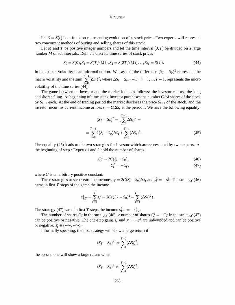
Let S= S(t) be a function representing evolution of a stock price. Two experts will representtwo concurrent methods of buying and selling shares of this stock.

Let M andT be positive integer numbers and let the time interval[0,T] be divided on a largenumberM of subintervals. Define a discrete time series of stock prices

S0 = S(0),S1 = S(T/(M)),S2 = S(2T/(M)) . . . ,SM = S(T). (44)

In this paper, volatility is an informal notion. We say that the difference(ST −S0)2 represents the

macro volatility and the sumT−1∑

i=0(∆Si)

2, where∆Si = Si+1−Si , i = 1, . . .T −1, represents the micro

volatility of the time series (44).The game between an investor and the market looks as follows: the investor can use the long

and short selling. At beginning of time stept Investor purchases the numberCt of shares of the stockby St−1 each. At the end of trading period the market discloses the priceSt+1 of the stock, and theinvestor incur his current income or lossst =Ct∆St at the periodt. We have the following equality

(ST −S0)2 = (

T−1

∑t=0

∆St)2 =

=T−1

∑t=0

2(St −S0)∆St +T−1

∑t=0

(∆St)2. (45)

The equality (45) leads to the two strategies for investor which are represented by two experts. Atthe beginning of stept Experts 1 and 2 hold the number of shares

C1t = 2C(St −S0), (46)

C2t =−C1

t , (47)

whereC is an arbitrary positive constant.These strategies at stept earn the incomess1

t = 2C(St −S0)∆St ands2t =−s1

t . The strategy (46)earns in firstT steps of the game the income

s11:T =

T

∑t=1

s1t = 2C((ST −S0)

2−T−1

∑t=1

(∆St)2).

The strategy (47) earns in firstT steps the incomes21:T =−s1

1:T .The number of sharesC1

t in the strategy (46) or number of sharesC2t =−C1

t in the strategy (47)can be positive or negative. The one-step gainss1

t ands2t =−s1

t are unbounded and can be positiveor negative:si

t ∈ (−∞,+∞).Informally speaking, the first strategy will show a large return if

(ST −S0)2 ≫

T−1

∑i=0

(∆Si)2;

the second one will show a large return when

(ST −S0)2 ≪

T−1

∑i=0

(∆Si)2.

258


0 50 100 150 200 250 300 350 400130

135

140

145

150

155

160

165

170

175

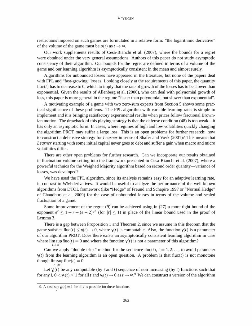
Figure 4: Evolution of Gazprom stock price

There is an uncertainty domain for these strategies, that is, a case when both≫ and≪ do not hold.The idea of these strategies is based on the paper of Cheredito (2003) (see also Rogers 1997 andDelbaen and Schachermayer 1994 ) who have constructed arbitrage strategies for a financial marketthat consists of money market account and a stock whose price follows a fractional Brownian motionwith drift or an exponential fractional Brownian motion with drift. Vovk (2003) has reformulatedthese strategies for discrete time. We use these strategies to define a mixed strategy which incurgain when macro and micro volatilities of time series differ. There is no uncertainty domain forcontinuous time.

We analyze this game in the decision theoretic online learning (DTOL) framework (Freund andSchapire, 1997). We introduceLearnerthat can choose between two strategies (46) and (47). Tochange from follow the leader framework to DTOL we derandomize the FPL algorithm PROT.7

We interpret the expected one-step gainE(st) gain as the weighted average of one-step gains ofexperts strategies. In more detail, at each stept, Learnerdivide his investment in proportion to theprobabilities of expert strategies (46) and (47) computed by the FPL algorithm and suffers the gain

Gt = 2C(St −S0)(P{It = 1}−P{It = 2})∆St

at any stept, whereC is an arbitrary positive constant;G1:T = ∑Tt=1Gt = E(s1:T) is theLearner’s

cumulative gain.

7. To apply Theorem 2 we interpreted gain as a negative loss.

259

V’ YUGIN

0 50 100 150 200 250 300 350 4000

0.05

0.1

0.15

0.2

0.25

0.3

0.35

0.4

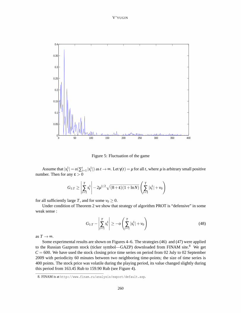
Figure 5: Fluctuation of the game

Assume that|s1t |= o(∑t

i=1 |s1i |) ast →∞. Letγ(t) = µ for all t, whereµ is arbitrary small positive

number. Then for anyε > 0

G1:T ≥∣

∣

∣

∣

∣

T

∑t=1

s1t

∣

∣

∣

∣

∣

−2µ1/2√

(8+ ε)(1+ lnN)

(

T

∑t=1

|s1t |+v0

)

for all sufficiently largeT, and for somev0 ≥ 0.Under condition of Theorem 2 we show that strategy of algorithm PROT is “defensive” in some

weak sense :

G1:T −∣

∣

∣

∣

∣

T

∑t=1

s1t

∣

∣

∣

∣

∣

≥−o

(

T

∑t=1

|s1t |+v0

)

(48)

asT → ∞.Some experimental results are shown on Figures 4–6. The strategies (46)and (47) were applied

to the Russian Gazprom stock (ticker symbol—GAZP) downloaded from FINAM site.8 We getC= 600. We have used the stock closing price time series on period from 02 Julyto 02 September2009 with periodicity 60 minutes between two neighboring time-points; the size of timeseries is400 points. The stock price was volatile during the playing period, its value changed slightly duringthis period from 163.45 Rub to 159.90 Rub (see Figure 4).

8. FINAM is athttp://www.finam.ru/analysis/export/default.asp.

260


0 50 100 150 200 250 300 350 400−1

0

1

2

3

4

5x 10

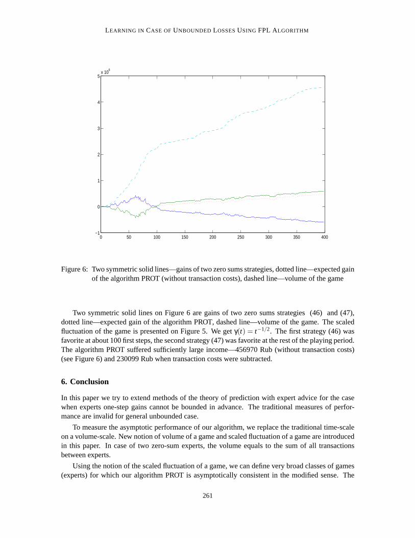
6

Figure 6: Two symmetric solid lines—gains of two zero sums strategies, dotted line—expected gainof the algorithm PROT (without transaction costs), dashed line—volume of thegame

Two symmetric solid lines on Figure 6 are gains of two zero sums strategies (46)and (47),dotted line—expected gain of the algorithm PROT, dashed line—volume of the game. The scaledfluctuation of the game is presented on Figure 5. We getγ(t) = t−1/2. The first strategy (46) wasfavorite at about 100 first steps, the second strategy (47) was favorite at the rest of the playing period.The algorithm PROT suffered sufficiently large income—456970 Rub (without transaction costs)(see Figure 6) and 230099 Rub when transaction costs were subtracted.

6. Conclusion

In this paper we try to extend methods of the theory of prediction with expert advice for the casewhen experts one-step gains cannot be bounded in advance. The traditional measures of perfor-mance are invalid for general unbounded case.

To measure the asymptotic performance of our algorithm, we replace the traditional time-scaleon a volume-scale. New notion of volume of a game and scaled fluctuation of a game are introducedin this paper. In case of two zero-sum experts, the volume equals to the sumof all transactionsbetween experts.

Using the notion of the scaled fluctuation of a game, we can define very broad classes of games(experts) for which our algorithm PROT is asymptotically consistent in the modified sense. The

261

V’ YUGIN

restrictions imposed on such games are formulated in a relative form: “the logarithmic derivative”of the volume of the game must beo(t) ast → ∞.

Our work supplements results of Cesa-Bianchi et al. (2007), where thebounds for a regretwere obtained under the very general assumptions. Authors of this paper do not study asymptoticconsistency of their algorithm. Our bounds for the regret are defined in terms of a volume of thegame and our learning algorithm is asymptotically consistent in the mean and almostsurely.

Algorithms for unbounded losses have appeared in the literature, but none of the papers dealwith FPL and “fast-growing” losses. Looking closely at the requirements of this paper, the quantityfluc(t) has to decrease to 0, which to imply that the rate of growth of the losses has to be slower thanexponential. Given the results of Allenberg et al. (2006), who can dealwith polynomial growth ofloss, this paper is more general in the regime “faster than polynomial, but slower than exponential”.

A motivating example of a game with two zero-sum experts from Section 5 showssome prac-tical significance of these problems. The FPL algorithm with variable learningrates is simple toimplement and it is bringing satisfactory experimental results when prices follow fractional Brown-ian motion. The drawback of this playing strategy is that the defense condition(48) is too weak—ithas only an asymptotic form. In cases, where regimes of high and low volatilitiesquickly changingthe algorithm PROT may suffer a large loss. This is an open problems for further research: howto construct a defensive strategy forLearnerin sense of Shafer and Vovk (2001)? This means thatLearnerstarting with some initial capital never goes to debt and suffer a gain when macro and microvolatilities differ.

There are other open problems for further research. Can we incorporate our results obtainedin fluctuation-volume setting into the framework presented in Cesa-Bianchi et al. (2007), where apowerful technics for the Weighed Majority algorithm based on second order quantity—variance oflosses, was developed?

We have used the FPL algorithm, since its analysis remains easy for an adaptive learning rate,in contrast to WM-derivatives. It would be useful to analyze the performance of the well knownalgorithms from DTOL framework (like “Hedge” of Freund and Schapire 1997 or “Normal Hedge”of Chaudhuri et al. 2009) for the case of unbounded losses in terms ofthe volume and scaledfluctuation of a game.

Some improvement of the regret (9) can be achieved using in (27) a more tight bound of theexponenter ≤ 1+ r + (e− 2)r2 (for |r| ≤ 1) in place of the linear bound used in the proof ofLemma 3.

There is a gap between Proposition 1 and Theorem 2, since we assume in thistheorem that thegame satisfies fluc(t) ≤ γ(t)→ 0, whereγ(t) is computable. Also, the functionγ(t) is a parameterof our algorithm PROT. Does there exists an asymptotically consistent learning algorithm in casewhere limsup

t→∞fluc(t) = 0 and where the functionγ(t) is not a parameter of this algorithm?

Can we apply “double trick” method for the sequence fluc(t), t = 1,2, . . ., to avoid parameterγ(t) from the learning algorithm is an open question. A problem is that fluc(t) is not monotonethough limsup

t→∞fluc(t) = 0.

Let γi(t) be any computable (byi andt) sequence of non-increasing (byt) functions such thatfor anyi, 0< γi(t)≤ 1 for all t andγi(t)→ 0 ast → ∞.9 We can construct a version of the algorithm

9. A case supi

γi(t) = 1 for all t is possible for these functions.

262


PROT which is asymptotically consistent in the mean for any game satisfying

limsupt→∞

fluc(t)γi(t)

< ∞ (49)

for somei. To solve this problem define a computable non-increasing functionγ(t) such that

• 0< γ(t)≤ 1,

• γ(t)→ 0 ast → ∞,

• for any i there exists anti such thatγ(t)≥ γi(t) for all t ≥ ti .

Evidently, the algorithm PROT with the parameterγ(t) is asymptotically consistent in the mean forany game such that (49) holds for somei.

We consider in this paper only the full information case. An analysis of theseproblems underpartial monitoring is a subject for a further research.

Acknowledgments

This research was partially supported by Russian foundation for fundamental research: 09-07-00180-a and 09-01-00709a.

Appendix A. Proof of Lemma 7

The proof of Lemma 7 is based on Kolmogorov’s theorem on three series and its corollaries. Forcompleteness of presentation we reconstruct the proof from Petrov (1975) (Chapter IX, Section 2).

For any random variableX and a positive numberc denote

Xc =

{

X if |X| ≤ c0 otherwise.

The Kolmogorov’s theorem on three series says:For any sequence of independent random variablesXt , t = 1,2, . . ., the following implications

hold

• If the series∑∞t=1Xt is convergent almost surely then the series∑∞

t=1EXct , ∑∞

t=1DXct and

∑∞t=1P{|Xt | ≥ c} are convergent for eachc > 0, whereE is the mathematical expectation

andD is the variation.

• The series∑∞t=1Xt is convergent almost surely if all these series are convergent for somec> 0.

See Shiryaev (1980) for the proof.Assume conditions of Lemma 7 hold. We will prove that

∞

∑t=1

Eg(Xt)

g(at)< ∞ (50)

263

V’ YUGIN

implies

∞

∑t=1

Xt

at< ∞

almost surely. From this, by Kroneker’s lemma 10 (see below), the series

1at

∞

∑t=1

Xt (51)

is convergent almost surely.Let Vt be a distribution function of the random variableXt . Sinceg non-increases,

P{|Xt |> at} ≤∫|x|≥at

g(x)g(at)

dVt(x)≤Eg(Xt)

g(at).

Then by (50)

∞

∑t=1

P

{∣

∣

∣

∣

Xt

at

∣

∣

∣

∣

≥ 1

}

< ∞ (52)

almost surely. Denote

Zt =

{

Xt if |Xt | ≤ at

0 otherwise.

By definitionx2/g(x))≤ at/g(at) for |x|< at . Rearranging, we obtainx2/at ≤ g(x)/g(at) for thesex. Therefore,

EZ2t =

∫

|x|<at

x2dVt(x)≤a2

t

g(at)

∫

|x|<at

g(x)dVt(x)≤a2

t

g(at)Eg(Xt).

By (50) we obtain

∞

∑t=1

E

(

Zt

at

)2

< ∞. (53)

SinceEXt =∞∫

−∞xdVt(x) = 0,

|EZt |=

∣

∣

∣

∣

∣

∣

∫

|x|>at

xdVt(x)

∣

∣

∣

∣

∣

∣

≤ at

g(at)

∫

|x|>at

g(x)dVt(x)≤at

g(at)Eg(Xt). (54)

By (50)∞

∑t=1

E

(

Xt

at

)1

≤∞

∑t=1

∣

∣

∣

∣

E

(

Zt

at

)∣

∣

∣

∣

< ∞.

From (52)–(54) and the theorem on three series we obtain (51).We have used Toeplitz and Kroneker’s lemmas.

264


Lemma 9 (Toeplitz) Let xt be a sequence of real numbers and bt be a sequence of nonnegative real

numbers such that at =t∑

i=1bi → ∞, xt → x and|x|< ∞. Then

1at

t

∑i=1

bixi → x. (55)

Proof. For anyε > 0 antε exists such that|xt −x|< ε for all t ≥ tε. Then∣

∣

∣

∣

∣

1at

t

∑I=1

bi(xi −x)

∣

∣

∣

∣

∣

≤ 1at

∑i<tε

|bi(xi −x)|+ ε

for all t ≥ tε. Sinceat → ∞, we obtain (55).

Lemma 10 (Kroneker) Assume∞∑

t=1xt < ∞ and at → ∞ Then

1at

t

∑i=1

aixi → 0.

The proof is the straightforward corollary of Toeplitz lemma.

References

C. Allenberg, P. Auer, L. Gyorfi and Gy. Ottucsak. Hannan consistency in on-Line learning in case ofunbounded losses under partial monitoring. In Jose L. Balcazar, Philip M. Long, Frank Stephan,editors,Proceedings of the 17th International Conference ALT 2006, Lecture Notes in ComputerScience 4264, pages 229–243, Springer-Verlag, Berlin, Heidelberg, 2006.

K. Chaudhuri, Y. Freund and D. Hsu. A parameter-free hedging algorithm. Technical ReportarXiv:0903.2851v1 [cs.LG], March 2009.

P. Cheredito. Arbitrage in fractional Brownian motion.Finance and Statistics, 7:533–553, 2003.

N. Cesa-Bianchi, Y. Mansour and G. Stoltz. Improved second-order bounds for prediction withexpert advice.Machine Learning, 66(2–3):321–352, 2007.

F. Delbaen and W. Schachermayer. A general version of the fundamental theorem of asset pricing.Mathematische Annalen, 300:463–520, 1994.

Y. Freund and R.E. Schapire. A decision-theoretic generalization of on-line learning and an appli-cation to boosting.Journal of Computer and System Sciences, 55:119–139, 1997.

J. Hannan. Approximation to Bayes risk in repeated plays. In M. Dresher, A.W. Tucker, and P.Wolfe, editors,Contributions to the Theory of Games 3, pages 97-139, Princeton UniversityPress, 1957.

M. Hutter and J. Poland. Prediction with expert advice by following the perturbed leader for generalweights. In S.Ben-Dawid, J.Case, A.Maruoka, editorsProceedings of the 15th International Con-ference ALT 2004, Lecture Notes in Artificial Intelligence 3244, pages 279–293, Springer-Verlag,Berlin, Heidelberg, 2004.

265

V’ YUGIN

M. Hutter and J. Poland. Adaptive online prediction by following the perturbed leader.Journal ofMachine Learning Research, 6:639–660, 2005.

A. Kalai and S. Vempala. Efficient algorithms for online decisions. In Bernhard Scholkopf, ManfredK. Warmuth, editors,Proceedings of the 16th Annual Conference on Learning Theory COLT2003, Lecture Notes in Computer Science 2777, pages 506–521, Springer-Verlag, Berlin, 2003.Extended version inJournal of Computer and System Sciences, 71:291–307, 2005.

N. Littlestone and M.K. Warmuth. The weighted majority algorithm.Information and Computation,108:212–261, 1994.

G. Lugosi and N. Cesa-Bianchi.Prediction, Learning and Games. Cambridge University Press,New York, 2006.

V.V. Petrov. Sums of independent random variables.Ergebnisse der Mathematik und Ihrer Gren-zgebiete, Band 82, Springer-Verlag, New York, Heidelberg, Berlin, 1975.

J. Poland and M. Hutter. Defensive universal learning with experts for general weights. In S.Jain,H.U.Simon and E.Tomita, editors,Proceedings of the 16th International Conference ALT 2005,Lecture Notes in Artificial Intelligence 3734, pages 356–370, Springer-Verlag, Berlin, Heidel-berg, 2005.

C. Rogers. Arbitrage with fractional Brownian motion.Mathematical Finance, 7:95–105, 1997.

G. Shafer and V. Vovk.Probability and Finance. It’s Only a Game!, Wiley, New York, 2001.

A.N. Shiryaev.Probability. Springer-Verlag, Berlin, 1980.

V. Vovk. Aggregating strategies. In M. Fulk and J. Case, editors,Proceedings of the 3rd AnnualWorkshop on Computational Learning Theory, pages 371–383, Morgan Kaufmann, San Mateo,CA, 1993.

V. Vovk. A game-theoretic explanation of the√

dt effect. Working paper #5, Available online athttp://www.probabilityandfinance.com, 2003.

V.V. V’yugin. The follow perturbed leader algorithm protected from unbounded one-step losses. InRicard Gavalda, Gabor Lugosi, Thomas Zeugmann, and Sandra Zilles, editors, Proceedings ofthe 20th International Conference ALT 2009, Lecture Notes in Artificial Intelligence 5809, pages.38-52, Springer-Verlag, Berlin Heidelberg, 2009.

V.V. V’yugin. Learning volatility of discrete time series using prediction with expert advice. In O.Watanabe and T. Zeugmann, editors,SAGA 2009, Lecture Notes in Computer Science 5792, pages16-30, Springer-Verlag, Berlin, Heidelberg, 2009.

266

Online Learning in Case of Unbounded Losses Using Follow the

Documents

Transcript of Online Learning in Case of Unbounded Losses Using Follow the