Proof Spaces for Unbounded Parallelism

Azadeh Farzan Zachary KincaidUniversity of Toronto

Andreas PodelskiUniversity of Freiburg

AbstractIn this paper, we present a new approach to automatically ver-ify multi-threaded programs which are executed by an unboundednumber of threads running in parallel.

The starting point for our work is the problem of how we canleverage existing automated verification technology for sequentialprograms (abstract interpretation, Craig interpolation, constraintsolving, etc.) for multi-threaded programs. Suppose that we aregiven a correctness proof for a trace of a program (or for someother program fragment). We observe that the proof can alwaysbe decomposed into a finite set of Hoare triples, and we ask whatcan be proved from the finite set of Hoare triples using only simplecombinatorial inference rules (without access to a theorem proverand without the possibility to infer genuinely new Hoare triples)?

We introduce a proof system where one proves the correctnessof a multi-threaded program by showing that for each trace of theprogram, there exists a correctness proof in the space of proofs thatare derivable from a finite set of axioms using simple combinatorialinference rules. This proof system is complete with respect to theclassical proof method of establishing an inductive invariant (whichuses thread quantification and control predicates). Moreover, it ispossible to algorithmically check whether a given set of axiomsis sufficient to prove the correctness of a multi-threaded program,using ideas from well-structured transition systems.

1. IntroductionIn this paper, we present a new approach to verifying multi-threaded programs which are executed by an unbounded number ofconcurrent threads. Many important systems and application pro-grams belong to this category, e.g. filesystems, device drivers, webservers, and image processing applications.

We will start by demonstrating our approach on a simple exam-ple. Consider a program in which an unknown number of threadsconcurrently execute the code below. The goal is to verify that, ifg ≥ 1 holds initially, then it will always hold (regardless of howmany threads are executing).

global int glocal int x1: x := g;2: g := g+x;

Consider the set of the Hoare triples (A) - (D) given below.Permission to make digital or hard copies of all or part of this work for personal orclassroom use is granted without fee provided that copies are not made or distributedfor profit or commercial advantage and that copies bear this notice and the full citationon the first page. Copyrights for components of this work owned by others than theauthor(s) must be honored. Abstracting with credit is permitted. To copy otherwise, orrepublish, to post on servers or to redistribute to lists, requires prior specific permissionand/or a fee. Request permissions from permissions@acm.org.POPL’15, January 15 - 17 2015, Mumbai, India.Copyright is held by the owner/author(s). Publication rights licensed to ACM.ACM 978-1-4503-3300-9/15/01. . . $15.00.http://dx.doi.org/10.1145/2676726.2677012

(A) {g ≥ 1} 〈x := g : 1〉 {x(1) ≥ 1}(B) {g ≥ 1 ∧ x(1) ≥ 1} 〈g := g + x : 1〉 {g ≥ 1}(C) {g ≥ 1} 〈x := g : 1〉 {g ≥ 1}(D) {x(1) ≥ 1} 〈x := g : 2〉 {x(1) ≥ 1}

Here we use x(1) to refer to Thread 1’s copy of the local variablex, and 〈x := g : 1〉 to indicate the instruction x := g executed byThread 1.

We will discuss how such Hoare triples can be generated au-tomatically shortly. But for now, suppose that we have been giventhe above set of Hoare triples, and consider a deductive system inwhich these triples are taken as axioms, and the only rules of infer-ence are sequencing, symmetry, and conjunction. These rules areeasily illustrated with concrete examples:

• Sequencing composes two Hoare triples sequentially. For ex-ample, sequencing (A) and (D) yields

(A ◦ D) {g ≥ 1} 〈x := g : 1〉〈x := g : 2〉 {x(1) ≥ 1}

• Symmetry permutes thread identifiers. For example, renaming(A) and (C) (mapping 1 7→ 2) yields

(A’) {g ≥ 1} 〈x := g : 2〉 {x(2) ≥ 1}(C’) {g ≥ 1} 〈x := g : 2〉 {g ≥ 1}

and, renaming (D) (mapping 1 7→ 2 and 2 7→ 1) yields

(D’) {x(2) ≥ 1} 〈x := g : 1〉 {x(2) ≥ 1}

• Conjunction composes two Hoare triples by conjoining pre- andpostconditions. For example, conjoining (A’) and (C’) yields

(A’ ∧ C’) {g ≥ 1} 〈x := g : 2〉 {g ≥ 1 ∧ x(2) ≥ 1}

and conjoining (A) and (D’) yields (A ∧ D’)

{g ≥ 1 ∧ x(2) ≥ 1} 〈x := g : 1〉 {x(1) ≥ 1 ∧ x(2) ≥ 1}

Naturally, the deductive system may apply inference rules todeduced Hoare triples as well: for example, by sequencing (A’∧C’)and (A ∧ D’), we get the Hoare triple

{g ≥ 1} 〈x := g : 2〉〈x := g : 1〉 {x(1) ≥ 1 ∧ x(2) ≥ 1}

A proof space is a set of valid Hoare triples which is closed undersequencing, symmetry, and conjunction (that is, it is a theory of thisdeductive system). Any finite set of valid Hoare triples generates aninfinite proof space by considering those triples to be axioms andtaking their closure under deduction; we call such a finite set ofHoare triples a basis for the generated proof space.

One key insight in this paper is that, although it may be chal-lenging to formalize a correctness argument for a multi-threadedprogram, any given trace (sequence of program instructions) of theprogram is just a simple (straight-line) sequential program which

can be easily proved correct. In fact, just these three simple infer-ence rules (sequencing, symmetry, and conjunction) are sufficientto prove the correctness of any trace of the example program. Thatis, for any trace τ of the program, {g ≥ 1} τ {g ≥ 1} belongsto the proof space generated by (A) − (D), regardless of which orhow many threads execute in τ . Crucially (and due to the simplic-ity of the inference rules), this fact can be checked completely au-tomatically, by leveraging techniques developed in the context ofwell-structured transition systems [2, 17, 18].

Now let us turn to the problem of how Hoare triples like (A) −(D) can be generated automatically. An important feature of proofspaces is that they are generated from a very simple set of Hoaretriples, of the sort one could expect to generate using standard tech-nology for sequential verification. To appreciate the simplicity ofthese triples, consider the following inductive invariant for the pro-gram, the classical notion of correctness proof for multi-threadedprograms:

g ≥ 1 ∧ (∀i.loc(i) = 2⇒ x(i) ≥ 1)

(which indicates that g is at least 1, and all threads i at line 2 ofthe program have x(i) at least 1). This is a simple invariant forthis program, but it is one which we cannot rely on a sequentialverifier to find because it makes use of features which are notencountered on sequential programs: thread quantification (∀i), andcontrol predicates (loc(i) = 2). In contrast, the triples (A) − (D)are of the form one might expect to generate using a sequentialverifier. Thus, proof spaces are a solution to the problem of how touse automated proof technology for sequential programs to provethe correctness of programs with unboundedly many threads.

One possible algorithm (discussed further in Section 7) for au-tomating proof spaces is to build a basis for a proof space iterativelyin a manner analogous to a counter-example guided abstraction re-finement (CEGAR) loop. While this algorithm is not the focus ofthis paper, it is important to recognize the context of and motivationbehind proof spaces. The algorithm operates as follows: first choosea trace for which there is no correctness theorem in the proof space.For example, suppose that we start with the trace

〈x := g : 1〉〈x := g : 2〉〈g := g + x : 1〉

{g ≥ 1}〈x := g : 1〉{x(1) ≥ 1}〈x := g : 2〉{x(1) ≥ 1}〈g := g + x : 1〉{g ≥ 1}

This trace can be viewed as a sequentialprogram, and we can use standard technology(e.g., abstract interpretation, constraint solv-ing, Craig interpolation) to construct a prooffor it (for example, the one on the right). Byextracting the atomic Hoare triples along thissequence, we can arrive at the triples (A), (B),and (D), which we add to our basis. We maythen extract a new trace which cannot be proved using just (A), (B),and (D), and restart the loop. The loop terminates when (and if) (1)it finds a feasible counter-example or (2) all traces of the programhave correctness theorems in the proof space.

The key contribution of this paper is the notion of proof spaces,a proof system which can be used to exploit sequential verificationtechnology for proving the correctness of multi-threaded programswith unboundedly many threads. The merits of proof spaces are asfollows:

• Rather than enriching the language of assertions (introducingthread quantification and control predicates) and employingmore powerful symbolic reasoning, proof spaces use simple as-sertions which can be combined using combinatorial reasoning(i.e., without a theorem prover).• We show that the combinatorial reasoning involved in checking

whether all traces of a program have a correctness theorem ina proof space can be automated, and give an algorithm whichleverages ideas from well-structured transition systems [18].

We show that this proof space checking problem is undecidablein general, but our algorithm is a decision procedure for aninteresting subclass of proof spaces.• Despite the apparent weakness of our three inference rules and

the restricted language of assertions, we show that proof spacesare complete relative to a variant of Ashcroft’s classical proofsystem for multi-threaded programs (which employs universalthread quantification and control predicates).

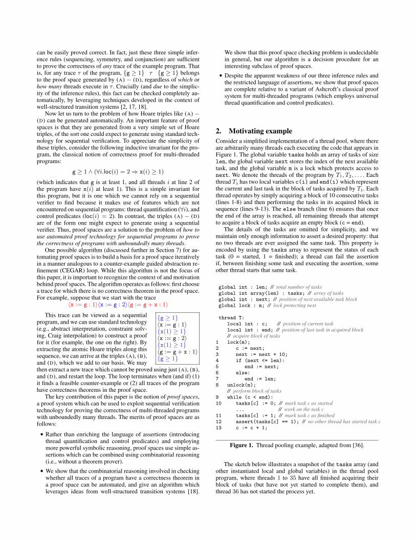
2. Motivating exampleConsider a simplified implementation of a thread pool, where thereare arbitrarily many threads each executing the code that appears inFigure 1. The global variable tasks holds an array of tasks of sizelen, the global variable next stores the index of the next availabletask, and the global variable m is a lock which protects access tonext. We denote the threads of the program by T1, T2, . . . . Eachthread Ti has two local variables c(i) and end(i) which representthe current and last task in the block of tasks acquired by Ti. Eachthread operates by simply acquiring a block of 10 consecutive tasks(lines 1-8) and then performing the tasks in its acquired block insequence (lines 9-13). The else branch (line 6) ensures that oncethe end of the array is reached, all remaining threads that attemptto acquire a block of tasks acquire an empty block (c = end).

The details of the tasks are omitted for simplicity, and wemaintain only enough information to assert a desired property: thatno two threads are ever assigned the same task. This property isencoded by using the tasks array to represent the status of eachtask (0 = started, 1 = finished); a thread can fail the assertionif, between finishing some task and executing the assertion, someother thread starts that same task.

global int : len; // total number of tasksglobal int array(len) : tasks; // array of tasksglobal int : next; // position of next available task blockglobal lock : m; // lock protecting next

thread T:local int : c; // position of current tasklocal int : end; // position of last task in acquired block// acquire block of tasks

1 lock(m);2 c := next;3 next := next + 10;4 if (next <= len):5 end := next;6 else:7 end := len;8 unlock(m);

// perform block of tasks9 while (c < end):10 tasks[c] := 0; // mark task c as started

... // work on the task c11 tasks[c] := 1; // mark task c as finished12 assert(tasks[c] == 1); // no other thread has started task c13 c := c + 1;

Figure 1. Thread pooling example, adapted from [36].

The sketch below illustrates a snapshot of the tasks array (andother instantiated local and global variables) in the thread poolprogram, where threads 1 to 35 have all finished acquiring theirblock of tasks (but have not yet started to complete them), andthread 36 has not started the process yet.

Locking

{true}

Initialization

{true} {c(1) ≤ next} {true}〈lock(m) : 1〉 〈c := next : 1〉 〈next := next + 10 : 1〉 〈end := next : 1〉{m = 1} {c(1) ≤ next} {c(1) < next} {end(1) ≤ next}

{m = 1} {end(1) ≤ next} {true} {len ≤ next}〈lock(m) : 1〉 〈c := next : 2〉 〈assume(next > len) : 1〉 〈end := len : 1〉{false} {end(1) ≤ c(2)} {len ≤ next} {end(1) ≤ next}

Loop

{true} {true} {tasks[c(1)] = 1} {end(1) ≤ c(2)}〈assume(c < end) : 1〉 〈tasks[c] := 1 : 1〉 〈assume(tasks[c] != 1) : 1〉 〈c := c + 1 : 2〉{c(1) < end(1)} {tasks[c(1)] = 1} {false} {end(1) ≤ c(2)}

{tasks[c(1)] = 1 ∧ c(1) < end(1) ≤ c(2)} {tasks[c(1)] = 1 ∧ c(2) < end(2) ≤ c(1)}〈tasks[c] := 0 : 2〉 〈tasks[c] := 0 : 2〉{tasks[c(1)] = 1} {tasks[c(1)] = 1}

Figure 2. The basis of a proof space for the thread pooling example. The variable c(1) denotes the copy of the local variable c in Thread 1and the command 〈c := next : 1〉 denotes the instance of the command c := next in Thread 1, etc. Trivial Hoare triples of the type{ϕ} 〈σ : i〉 {ϕ} where the set of variables that 〈σ : i〉 modifies is disjoint from the set of variables in ϕ, have been omitted for brevity.

c(1)

end(1)

c(2)

end(2)

c(35)

end(35) len

next

. . . . . .

c(3)

end(34)

In order to show that two threads, say Threads 1 and 2, cannot beassigned the same task, we may argue that the intervals assignedto them [c(1), end(1)) and [c(2), end(2)) are disjoint byproving that end(1) is less than or equal to c(2).

Proof space for thread pooling Figure 2 illustrates a finite setof Hoare triples (a basis) that generates a proof space for thethread pooling program. In the figure, the Hoare triples are cate-gorized into three groups (Locking, Initialization, and Loop). Weomit Hoare triples that represent trivial invariance axioms of theform {ϕ} 〈σ : i〉 {ϕ} where the command 〈σ : i〉 does not writeto a variable that appears in ϕ; for example,

{c(2) ≤ next} 〈c := next : 1〉 {c(2) ≤ next} .Note that the set of triples in Figure 2 use mixed assertions (in

the terminology in [12]), which relate the values of local variablesto global variables (e.g., c(1) ≤ next), as well as inter-threadassertions, which relate the local variables of different threads (e.g.,end(1) ≤ c(2)). As discussed in [25], both mixed assertions andinter-thread assertions raise an issue when one attempts to usepredicate abstraction techniques. Inter-thread assertions cannot beused in classical compositional proof systems (e.g. thread-modularproofs). In these proof systems, inter-thread relationships can onlybe accommodated through auxiliary variables [29, 35].

To represent the program in a simple formal model, we en-code each conditional branch as a nondeterministic branch betweenassume commands (one for the condition and one for its negation),and we encode assert(e) through a command assume(!e) (forthe negation of the expression e) which leads to a new error loca-tion. We thus encode the correctness of the program (the validityof the assert statement) through the non-reachability of the errorlocation by any thread. An error trace is an interleaved sequence

of commands of any number of threads which leads some thread tothe error location (e.g., in Figure 3, the sequence in (a) followed bythe sequence in (b)). Thus, we can express the correctness of theprogram by the validity of the Hoare triple {true} τ {false} forevery error trace τ . Given this Hoare triple as the specification ofcorrectness of a trace, we have that a trace is correct if and only ifit is infeasible.

Let us now demonstrate how the proof space is used to arguefor the correctness of the program. We must show that for everyerror trace τ there exists a derivation of {true} τ {false}which can be constructed from the triples in Figure 2 using onlythe combinatorial inference rules of symmetry, conjunction, andsequencing.

Let us first consider the pair of Hoare triples in the Lockinggroup. We treat the lock(m) command as the atomic sequence{assume(m = 0); m := 1}, and unlock(m) command as theassignment m := 0. Intuitively, the locking Hoare triples encap-sulate the reasoning required to prove that the lock m provides mu-tually exclusive access to the variable next. Any trace that violatesthe locking semantics can be proved infeasible using the Hoaretriples in the Locking group along with the sequencing and sym-metry rules. To see why, consider that any such trace can be de-composed as

τ1 · 〈lock(m) : i〉 · τ2 · 〈lock(m) : j〉 · τ3

such that the following Hoare triples are valid:

{true} τ1 {true}{true} 〈lock(m) : i〉 {m = 1}{m = 1} τ2 {m = 1}{m = 1} 〈lock(m) : j〉 {false}{false} τ3 {false}

This decomposition exploits the fact that any trace which violatesthe semantics of locking has a shortest prefix which contains aviolation: that is, we may assume that τ2 contains no unlock(m)commands because, if it did, there would be a shorter prefix in

which two threads simultaneously hold the lock m. Having justifiedtheir semantic validity, we may now consider how to derive thesetriples using symmetry and sequencing from the Locking axioms inFigure 2. The two triples above concerning the lock(m) commandare inferred from the triples in the Locking group by renamingthread 1 (i.e. using the symmetry rule) to i and j, respectively.The rest of the triples come from the simple invariance Hoaretriples (not depicted in Figure 2, but mentioned in the caption),that allow us to infer {m = 1} 〈σ : i〉 {m = 1} for anycommand σ except unlock(m), and {true} 〈σ : i〉 {true} and{false} 〈σ : i〉 {false} for every command σ.

We now turn our attention to the error traces which do respectlocking semantics, and show that they are infeasible. The six Hoaretriples in the Initialization section of Figure 2 are sufficient to provethat after two threads (say 2 and 9) acquire their block of tasks,those blocks do not overlap (i.e., we have either end(9) ≤ c(2)or end(2) ≤ c(9), depending on the order in which the threadsacquire their tasks). An example of such a trace (which can beproved using just sequencing and symmetry operations) appears inFigure 3(a). We encourage the reader to show (using conjunction)that if we extend the trace in Figure 3(a) by the initializationsequence of a third thread (say, Thread 5) to obtain a trace τ , then

{true} τ {end(2) ≤ c(9) ∧ end(2) ≤ c(5) ∧ end(9) ≤ c(5)}belongs to the proof space as well. Following similar proof combi-nation steps, one can see that the argument can be adapted to traceswith any number of threads.

Finally, the triples in the Loop section can be used to showtwo things. First, the “non-overlapping” property established inthe initialization section is preserved by the loop: for example, ifend(2) ≤ c(9) holds at the beginning of the loop, then if thread 2or thread 9 (or any other thread) executes the loop, end(2) ≤ c(9)continues to hold. Second, (assuming the non-overlapping condi-tion holds), if some task has been completed then it remains com-pleted: for example, if tasks[c(2)] = 1, then when thread 9starts task c(9) (i.e. assigns 0 to tasks[c(9)]), it cannot over-write the value of the array cell tasks[c(2)] (this is ensured bythe precondition c(2) < end(2) ≤ c(9), which implies c(2) 6=c(9)). Figure 3(b) gives an example proof which can be derived us-ing the Loop section. The sequential composition of traces in Fig-ure 3(a) and Figure 3(b) forms an error trace (i.e. one that leads tothe error location), and sequencing their proofs yields a proof thatthe error trace is infeasible.

We hope that it is now intuitively clear (or at least plausible)that, given any particular error trace τ , it is possible to derive{true} τ {false} using the symmetry, sequencing, and conjunc-tion rules starting from the axioms given in Figure 2. The questionis: how can one be assured that all (infinitely many) error traces canbe proved infeasible in this way? In Section 6 we will show how toformalize such an argument, and moreover, give a procedure forchecking that it holds.

3. PreliminariesIn this section, we will define our program model and introducesome technical definitions.

We fix a set of global variables GV and a set of local variablesLV. Intuitively, these are the variables that can appear in the pro-gram text. We will often make use of the set LV × N of indexedlocal variables, and denote a pair 〈x, i〉 ∈ LV × N by x(i). Intu-itively, such an indexed local variable x(i) refers to thread i’s copyof the local variable x.

For simplicity, we will assume that program variables take in-teger values, and the program is expressible in the theory of linearinteger arithmetic. This assumption is made only to simplify thepresentation by making it more concrete; our approach and results

{true}lock(m) :2

{true}c := next :2

{true}next := next + 10 :2

{true}assume(next <= len) :2

{true}end := next :2

{end(2) � next}unlock(m) :2

{end(2) � next}lock(m) :9

{end(2) � next}c := next :9

{end(2) � c(9)}next := next + 10 :9

{end(2) � c(9)}assume(next <= len) :9

{end(2) � next}end := next :9

{end(2) � c(9)}unlock(m) :9

{end(2) � c(9)}

{end(2) � c(9)}assume(c < end) :2

{c(2) < end(2) � end(2) � c(9)}tasks[c] := 0 :2

{c(2) < end(2) � end(2) � c(9)}tasks[c] := 1 :2

{tasks[c(2)] = 1 � c(2) < end(2)� end(2) � c(9)}assume(c < end) :9

{tasks[c(2)] = 1 � c(2) < end(2)� end(2) � c(9)}tasks[c] := 0 :9

{tasks[c(2)] = 1}assume(tasks[c] != 1) :2

{false}

(a) Initialization example (b) Loop example

Figure 3. Example traces

do not depend on linear arithmetic in any essential way.Given a set of variable symbols V , we use Term(V ) to denote

the set of linear terms with variables drawn from V . Similarly,Formula(V ) denotes the set of linear arithmetic formulas withvariables drawn from V . We here use V as a parameter which wewill instantiate according to the context. For example, Term(GV ∪LV) denotes the set of terms which may appear in the text of aprogram (which refers to the thread template), and Formula(GV ∪(LV × N)) denotes the set of formulas which may appear in a pre-or postcondition (which refers to concrete threads).

We use the notation [x 7→ t] to denote a substitution whichreplaces the variable x with the term t and generalize the notationto parallel substitutions in the standard way. The application of asubstitution ρ to a formula ϕ (or a term t) is denoted ϕ[ρ] (or t[ρ]).Two classes of substitutions of particular interest for our technicaldevelopment are instantiations and permutations.

• Given an index i ∈ N, we use ιi to denote the instantiationsubstitution which replaces each local variable x ∈ LV with anindexed local variable x(i). For example, if we take i to be 3and c is a local variable and next is a global, we have

(c ≤ next)[ι3] = c(3) ≤ next

• Each permutation π : N → N defines a substitution which re-places each indexed local variable x(i) with x(π(i)). We abusenotation by identifying each permutation with the substitution itdefines. For example if π is a permutation which maps 3 ↔ 1,then

(c(3) ≤ next)[π] = c(1) ≤ next

We identify a program P with a control flow graph for a sin-gle thread template which is executed by an unbounded numberof threads. (The extension to more than one thread template isstraightforward.) A control flow graph is a directed, labeled graphP = 〈Loc,Σ, `init, `err, src, tgt〉, where Loc is a set of program lo-cations, Σ is a set of program commands, `init is a designated initiallocation, `err is a designated error location, and src, tgt : Σ→ Locare functions mapping each program command to its source and tar-get location. Note that our definition of a control flow graph (using

src and tgt) implies that we distinguish between different occur-rences of a program instruction.

A program command σ ∈ Σ is of one of two forms:

• an assignment of the form x := twhere x ∈ GV ∪ LV and t ∈ Term(GV ∪ LV), or• an assumption of the form assume(ϕ)

where ϕ ∈ Formula(GV ∪ LV).

We will denote a pair consisting of a program command σ ∈ Σand an index i ∈ N as the indexed command 〈σ : i〉. Intuitively,such an indexed command 〈σ : i〉 refers to thread i’s instance ofthe program command σ, or: the index i indicates the identifier ofthe thread which executes σ.

A trace

τ = 〈σ1 : i1〉〈σ2 : i2〉· · · 〈σn : in〉is a sequence of indexed commands.

A Hoare triple is a triple

{ϕ} τ {ψ}where τ is a trace and ϕ and ψ are formulas with global variablesand indexed local variables, i.e., ϕ,ψ ∈ Formula(GV∪ (LV×N)).

The validity of Hoare triples for traces is defined as one wouldexpect. Intuitively, if the command reads or writes the local vari-able x, then the indexed command 〈σ : i〉 (i.e., the command σexecuted by thread i) reads or writes thread i’s copy of the localvariable x. To express this formally, we use the instantiation sub-stitution ιi introduced above. In particular, if x is a local variable,x[ιi] is the indexed local variable x(i) (and if x is a global variable,x[ιi] is simply x).

For a trace of length 1 (i.e., for an indexed command), we have:

• {ϕ} 〈(x := t) : i〉 {ψ} is valid if

ϕ |= ψ[x[ιi] 7→ t[ιi]]

• {ϕ} 〈(assume(θ)) : i〉 {ψ} is valid if

ϕ ∧ θ[ιi] |= ψ

where |= denotes entailment modulo the theory of integer lin-ear arithmetic. For a trace of the form τ.〈σ : i〉, the triple{ϕ} τ.〈σ : i〉 {ψ} is valid if there exists some formula ψ′

such that {ϕ} τ {ψ′} and {ψ′} 〈σ : i〉 {ψ} are valid.We call a trace τ infeasible if the Hoare triple {true} τ {false}

is valid. Intuitively, τ is infeasible if it does not correspond to anyexecution.

Given a programP (identified by the control flow graph of a sin-gle thread template, i.e., a graph with edges labeled by commandsσ ∈ Σ and with the initial location `init and the error location `err),a trace τ is an error trace of P if

• for each index i ∈ N, the projection of τ onto the commandsof thread i corresponds to a path through P starting at `init (i.e.,each thread i starts at the initial location), and• there is (at least) one index j ∈ N such that the projection of τ

onto the commands of thread j corresponds to a path throughP ending at `err (i.e., some thread j ends at the error location).

We say that a program P is correct if every error trace of P isinfeasible (i.e., there is no execution of P wherein some threadreaches the error location `err).

The notion of correctness be used to encode many correctnessproperties including thread-state reachability (and thus the safetyof assert commands) and mutual exclusion. The encoding ispossibly done by introducing monitors (ghost instructions on ghostvariables), much in the same way that safety properties can bereduced to non-reachability in sequential programs.

4. Proof spacesWe will now introduce proof spaces, the central technical idea ofthis paper. We begin by formalizing the inference rules of SE-QUENCING, SYMMETRY, and CONJUNCTION.

The sequencing rule is a modification of the familiar one fromHoare logic. We omit the rule of consequence from Hoare logic,and instead incorporate consequence in our sequencing rule: thatis, we allow triples {ϕ0} τ0 {ϕ1} and {ϕ′1} τ1 {ϕ2} to becomposed when ϕ1 and ϕ′1 do not exactly match, but ϕ1 entails ϕ′1.However, a design goal of proof spaces is that the inference rulesshould be purely combinatorial (and thus, should not require accessto a theorem prover to discharge the entailment). Towards thisend, we define a combinatorial entailment relation on formulas:identifying a conjunction with the set of its conjuncts, we haveϕ ψ if ϕ is a superset of ψ. Formally,

ϕ1 ∧ ... ∧ ϕn ψ1 ∧ ... ∧ ψm if {ϕ1, ..., ϕn} ⊇ {ψ1, ..., ψm}The sequencing rule is formalized as follows:

SEQUENCING

{ϕ0} τ0 {ϕ1} ϕ1 ϕ′1 {ϕ′1} τ1 {ϕ2}{ϕ0} τ0 ; τ1 {ϕ2}

The symmetry rule exploits the fact that thread identifiers areinterchangeable in our program model, and therefore uniformlypermuting thread identifiers in a valid Hoare triple yields anothervalid Hoare triple:

SYMMETRY{ϕ} 〈σ1 : i1〉· · · 〈σn : in〉 {ψ}

{ϕ[π]} 〈σ1 : π(i1)〉· · · 〈σn : π(in)〉 {ψ[π]}π : N→ Nis a permutation

Lastly, the rule of conjunction allows one to combine two the-orems about the same trace by conjoining preconditions and post-conditions:

CONJUNCTION{ϕ1} τ {ψ1} {ϕ2} τ {ψ2}{ϕ1 ∧ ϕ2} τ {ψ1 ∧ ψ2}

Next, we formalize our notion of a proof space:

Definition 4.1 (Proof space) A proof space H is a set of validHoare triples which is closed under SEQUENCING, SYMMETRY,and CONJUNCTION. ⌟

Our definition restricts proof spaces to contain only valid Hoaretriples for the sake of convenience. Clearly, the SEQUENCING,SYMMETRY, and CONJUNCTION rules preserve validity.

The strategy behind using proof spaces as correctness proofscan be summarized in the following proof rule: If we can find aproof space H such that for every error trace τ of the program P ,we have that the Hoare triple {true} τ {false} belongs to H ,then P is correct.

Our main interest in proof spaces is using the above proof ruleas a foundation for algorithmic verification of concurrent programs.Towards this end, we augment the definition of proof spaces withadditional conditions that make them easier to manipulate algorith-mically. We call the proof spaces satisfying these conditions finitelygenerated proof spaces. First, we define basic Hoare triples, whichare the “generators” of such proof spaces.

Definition 4.2 (Basic Hoare triple) A basic Hoare triple is a validHoare triple of the form

{ϕ} 〈σ : i〉 {ψ}where

1. the postcondition ψ cannot be constructed by conjoining twoother formulas, and

2. for each j ∈ N, if an indexed local variable of the form x(j)appears in the precondition ϕ, then either j is equal to the indexi of the command, or x(j) or some other indexed local variabley(j) with the same index j must appear in the postcondition ψ(“the precondition mentions only relevant threads”). ⌟

The asymmetry between the precondition and the postconditionin Condition 1 is justified by the rule of consequence. Given a (non-basic) Hoare triple

{ϕ0 ∧ ϕ1} 〈σ : i〉 {ψ1 ∧ ψ2} ,we may “split the postcondition” to arrive at two valid triples

{ϕ0 ∧ ϕ1} 〈σ : i〉 {ψ1}{ϕ0 ∧ ϕ1} 〈σ : i〉 {ψ2}

from which the original triple may be derived via CONJUNCTION.As a result, the postcondition restriction on basic Hoare triples doesnot lose significant generality. Since preconditions cannot be splitin this way, Definition 4.2 is asymmetric.

Definition 4.3 (Finitely generated) We say that a proof space His finitely generated if there exists a finite set of basic Hoare triplesH such that H is the smallest proof space which contains H . Inthis situation, we call H a basis for H . ⌟

Proof spaces give a new proof system for verifying safety prop-erties for multi-threaded programs. The remainder of this paperstudies some of the questions which arise from introducing sucha proof system. In the next section, we consider the question of theexpressive power of proof spaces (that is, what can be proved usingproof spaces). In Sections 6 and 7, we discuss how proof spacesmay be used in the context of algorithmic verification.

5. CompletenessThe method of using global inductive invariants to prove correct-ness of concurrent programs dates back to the seminal work ofAshcroft [4]. Ashcroft’s method originally applied to programswith finitely many threads, but can be adapted to the infinite caseby admitting into the language of assertions universal quantifiersover threads. In this section, we prove the completeness of proofspaces relative to Ashcroft’s method. This establishes that the com-binatorial operations of proof spaces are adequate for represent-ing Ashcroft proofs, even though Ashcroft assertions make use offeatures not available to proof space assertions (namely, universalquantifiers over threads and control assertions).

We start by formalizing Ashcroft proofs. We can treat each localvariable as an uninterpreted function symbol of type N → Z (i.e,the interpretation of x ∈ LV is a function which maps each threadidentifier i ∈ N to the value of thread i’s copy of x).

We let TV be a set of thread variables which are variableswhose values range over the set of thread identifiers N. We typi-cally use i, j, i1, . . . to refer to thread variables (note that we usei, j, i1, . . . to refer to thread identifiers, i.e., elements of N). Weuse LV[TV] to denote the set of terms x(i) where x ∈ LV andi ∈ TV. A data assertion is a linear arithmetic formula ψ built upfrom global variables and terms of the form x(i) where x ∈ LV andi ∈ TV, i.e., ψ ∈ Formula(GV ∪ LV[TV]).

A global assertion is defined to be a sentence of the form

Φinv = ∀i1, ..., in.ϕinv(i1, ..., in)

where ϕinv is a formula built up from Boolean combinations of

• data assertions,• control assertions loc(i) = ` (with i ∈ TV and ` ∈ Loc), and• thread equalities i = j and disequalities i 6= j (with i, j ∈ TV).

For any program command σ ∈ Σ, we use JσK to denote thetransition formula which represents some thread executing σ. Thisis a formula over an extended vocabulary which includes a primedcopy of each of the global and local variable symbols (interpretedas the post-state values of those variables). This formula is of theform

∃i.ψ1(i) ∧ (∀j.ψ2(i, j))

where (intuitively) ψ1 describes the state change for the threadwhich executes σ (thread i), and ψ2 describes the state changefor all other threads (thread j). For example, if σ is an assignmentx := x + g where x is local, g is global, and ` = src(σ) and`′ = tgt(σ), then:JσK ≡ ∃i.

(loc(i) = ` ∧ loc′(i) = `′ ∧ x′(i) = x(i) + g ∧ g′ = g

∧∀j 6= i.(loc(j) = loc′(j) ∧ x(j) = x′(j)

)).

We may now formally define Ashcroft invariants:

Definition 5.1 (Ashcroft invariant) Given a program P , anAshcroft invariant is a global assertion Φinv such that

1. ∀i.loc(i) = `init entails Φinv.2. For any command σ ∈ Σ, we have that Φinv ∧ JσK entails

Φ′inv (where Φ′inv denotes the formula obtained by replacing thesymbols in Φinv with their primed copies)

3. Φinv entails ∀i.loc(i) 6= `err. ⌟

Clearly, the existence of an Ashcroft invariant for a programimplies its correctness (that is, that the error location of the programis unreachable). The following theorem is the main result of thissection, which establishes the completeness of proof spaces relativeto Ashcroft invariants.

Theorem 5.2 (Relative completeness) Let P be a program. Ifthere is an Ashcroft invariant which proves the correctness of P ,then there is a finitely generated proof space which proves thecorrectness of P . ⌟

Proof. To simplify notation, we will prove the result only for thecase that the Ashcroft proof has two quantified thread variables.The generalization to an arbitrary number of quantified threadvariables is straightforward.

Let P be a program, and let Φinv be an Ashcroft proof. Withoutloss of generality, we may assume that Φinv is written as

Φinv ≡(∀i∨`∈Loc

loc(i) = ` ∧ ϕ`(i))

∧(∀i 6= j.

∨`,`′∈Loc×Loc

loc(i) = ` ∧ loc(j) = `′ ∧ ϕ`,`′(i, j)))

where each ϕ`(i) and ϕ`,`′(i, j) is a integer arithmetic formula(i.e., does not contain loc). Furthermore, we can assume that Φinv

is symmetric in the sense that ϕ`,`′(i, j) is syntactically equal toϕ`′,`(j, i) and that ϕ`,`′(i, j) entails ϕ`(i) (for any i, j, `, `′). Wecan prove that any Φinv can be written in this form by inductionon Φinv We also assume that ϕ`err(i) = false and ϕ`init(i) =ϕ`init,`init(i, j) = true; the fact that this loses no generality is aconsequence of conditions 1 and 3 of Definition 5.1. Finally, weassume that each formula ϕ`(i) and ϕ`,`′(i, j) is not (syntactically)a conjunction (cf. Condition 1 of Definition 4.2): this assumptionis validated by observing any formula ϕ is equivalent to ϕ ∨ false,which is not a (syntactic) conjunction.

We construct a set of basic Hoare triples H by collecting the setof all Hoare triples of the following four types:

{ϕ`1(1)} 〈σ : 1〉 {ϕ`′1(1)}

{ϕ`1,`2(1, 2)} 〈σ : 1〉 {ϕ`2(2)}

{ϕ`1,`2(1, 2)} 〈σ : 1〉 {ϕ`′1,`2(1, 2)}

{ϕ`1,`2(1, 2) ∧ ϕ`1,`3(1, 3) ∧ ϕ`2,`3(2, 3)} 〈σ : 1〉 {ϕ`2,`3(2, 3)}where src(σ) = `1 and tgt(σ) = `′1.

We now must show that (1) each Hoare triple in H is ba-sic (i.e., satisfies Definition 4.2) and (2) for every trace τ of P ,{true} τ {false} belongs to the proof space generated by H .Condition (2) is delayed to Section 6, where we prove a strongerresult (Proposition 6.14). Here, we will just prove condition (1).

One can easily observe that conditions 1 and 2 of Definition 4.2hold. It remains to show that each Hoare triple in H is valid. Wewill prove only the validity of the Hoare triple

{ϕ`1,`2(1, 2)} 〈σ : 1〉 {ϕ`′1,`2(1, 2)}

where src(σ) = `1 and tgt(σ) = `′1. The other cases are similar.Let us write JσK as ∃i.ψ1(i) ∧ (∀k.ψ2(i, k)). For a proof by

contradiction, let us suppose that the above Hoare triple is invalid.This means:

ϕ`1,`2(1, 2) ∧ ψ1(1) ∧ (∀k.ψ2(1, k)) 6|= ϕ`′1,`2(1, 2)′

It follows that there exists a structure A such that

A |= ϕ`1,`2(1, 2) ∧ ψ1(1) ∧ (∀k.ψ2(1, k))

and A 6|= ϕ`′1,`2(1, 2)′. Without loss of generality, we may assumethat loc(2)A = loc′(2)A = `2. Our strategy will be to constructfrom A a structure B such that

B |= Φinv ∧ ψ1(1) ∧ (∀k.ψ2(1, k))

but B 6|= Φ′inv, which contradicts condition 2 of Definition 5.1.We obtain B simply by restricting the interpretation of the

Thread sort to the set {1, 2} (intuitively: we consider a configu-ration of the program in which 1 and 2 are the only threads). Thenwe have

B |= ϕ`1,`2(1, 2) ∧ ψ1(1) ∧ (∀k.ψ2(1, k))

by downward absoluteness of universal sentences and B 6|=ϕ`′1,`2(1, 2)′ by upward absoluteness of quantifier-free sentences.

From B |= ψ1(1), we have B |= loc(1) = `1. By assumption,we have B |= loc(2) = `2. It follows that

B |= ϕ`1,`2(1, 2) ∧ loc(1) = `1 ∧ loc(2) = `2

and thus, from the symmetry condition imposed on Φinv, that B |=Φinv. It is then easy to see that

B |= Φinv ∧ ψ1(1) ∧ (∀k.ψ2(1, k))

holds. Finally, we note that since B |= loc′(1) = `′1∧ loc′(2) = `2and B 6|= ϕ`′1,`2(1, 2), B is incompatible with every disjunct of∨

`,`′∈Loc×Loc

loc′(1) = ` ∧ loc′(2) = `′ ∧ ϕ′`,`′(1, 2)

and thus B 6|= Φ′inv.

As we mentioned previously, Ashcroft invariants are able tomake use of features which are not available to proof spaces,namely control assertions (i.e., assertions of the form loc(i) = `)and universal quantification over thread variables. These “exotic”features are typical for program logics for concurrent programswith unbounded parallelism. As a general rule, classical verifica-tion techniques for sequential programs do not synthesize asser-tions which make use of these features. The price we pay for therelative ease of generating proof spaces is the relative difficulty ofchecking them. We address this topic in the next section.

6. Proof checkingWe now turn to the main algorithmic problem suggested by theproof rule for proof spaces presented in Section 4: given a programP and a finite basis H of a proof space H , how do we checkwhether for every error trace τ we have that {true} τ {false}belongs to H ? Our solution to this problem begins by intro-ducing a new class of automata, predicate automata, which canbe used to represent both the set of error traces of a programand the set of traces τ which have the infeasibility theorem{true} τ {false} in a finitely generated proof space. We showthat the problem of checking whether for every error trace τ wehave that {true} τ {false} belongs to H can be reduced tothe emptiness problem for predicate automata. We show that thegeneral emptiness checking problem is undecidable, and we givea semi-algorithm and show that it is a decision procedure for aninteresting sub-class of predicate automata which correspond tothread-modular proofs.

6.1 Predicate automataPredicate automata are a class of infinite-state automata whichrecognize languages over an infinite alphabet of the form Σ × N.1

For readers familiar with alternating finite automata (AFA) [8, 9], ahelpful analogy might be that predicate automata are to first-orderlogic what AFA are to propositional logic. A predicate automaton(PA) is equipped with a relational vocabulary 〈Q, ar〉 (in the usualsense of first-order logic) consisting of a finite set of predicatesymbols Q and a function ar : Q→ N which maps each predicatesymbol to its arity. A state of a PA is a proposition q(i1, ..., iar(q)),where q ∈ Q and i1, ..., iar(q) ∈ N. The transition functionmaps such states to formulas in the vocabulary of the PA (wheredisjunction corresponds to nondeterministic (existential) choice,and conjunction corresponds to universal choice). It is importantto note that the symbols q ∈ Q are “uninterpreted”: they have nospecial semantics, and any subset of Nar(q) is a valid interpretationof q.

Given a vocabulary 〈Q, ar〉 (and given the set TV of threadvariables, i.e., variables whose values range over the set of threadidentifiers N), we define the set of positive formulas F(Q, ar)over 〈Q, ar〉 to be the set of negation-free formulas where eachatom is either (1) a proposition of the form q(i1, ..., in) (wherei1, ..., in ∈ TV), or (2) an equation i = j (where i, j ∈ TV), or(3) a disequation i 6= j (where i, j ∈ TV). Predicate automata aredefined as follows:

Definition 6.1 (Predicate automata) A predicate automaton (PA)is a 6-tuple A = 〈Q, ar,Σ, δ, ϕstart, F 〉 where

• 〈Q, ar〉 is a relational vocabulary• Σ is a finite alphabet• ϕstart ∈ F(Q, ar) is an initial formula with no free variables.• F ⊆ Q is a set of accepting predicate symbols• δ : Q × Σ → F(Q, ar) is a transition function which satisfies

the property that for any q ∈ Q and σ ∈ Σ, the free variablesof δ(q, σ) are members of the set {i0, ..., iar(q)}. ⌟

To understand the restriction on the variables in the formulaδ(q, σ), it may be intuitively helpful to think of q as q(i1, ..., iar(q))and of σ as 〈σ : i0〉.

We will elucidate this definition by first describing the dynamicsof a PA. PA dynamics will be defined by a nondeterministic2 tran-sition system where edges are labeled by elements of the indexed

1 Such languages are commonly called data languages [32].2 Readers familiar with AFA should note that we are effectively describingthe “nondeterminization” of PA.

alphabet Σ × N, and where the nodes of the transition system areconfigurations which we will introduce next:

Definition 6.2 (Configuration) LetA = 〈Q, ar,Σ, δ, ϕstart, F 〉 bea PA. A configuration C of A is finite set of ground propositions ofthe form q(i1, ..., iar(q)), where q ∈ Q and i1, ..., iar(q) ∈ N. ⌟

It is convenient to identify a configuration C with the formula∧q(i1,...,iar(q))∈C

q(i1, ..., iar(q)). We define the initial configura-tions of A to be the cubes of the disjunctive normal form (DNF) ofϕstart (for example, if ϕstart is p ∧ (q ∨ r), then the initial configu-rations are p ∧ q and p ∧ r). A configuration is accepting if for allq(i1, ..., iar(q)) ∈ C, we have q ∈ F ; otherwise, it is rejecting.

A PA A = 〈Q, ar,Σ, δ, ϕstart, F 〉 induces a transition relationon configurations as follows:

C σ:k−−→ C′

if C′ is a cube in the DNF of the formula∧q(i1,...,iar(q))∈C

δ(q, σ)[i0 7→ k, i1 7→ i1, ..., iar(q) 7→ iar(q)]

The fact that the free variables of δ(q, σ) must belong to the set{i0, ..., iar(q)} guarantees that the formula above has no free vari-ables, and therefore its DNF corresponds to a set of configurations.Note also that the formula above may contain equalities and dise-qualities, but since they are ground (have no free variables), theyare equivalent to either true or false, and thus can be eliminated.

We can think of δ(q, σ) as a rewrite rule whose applicationinstantiates the (implicit) formal parameters i1, ..., iar(q) of q to theactual parameters i1, ..., in and instantiates i0 to k (the index of theletter being read). In light of this interpretation, we will often writeδ in a form that makes the (implicit) formal parameters explicit: forexample, instead of

δ(q, σ) =(i0 6= i1 ∧ (q(i0, i1) ∨ q(i1, i2)))

∨ (i0 = i1 ∧ q(i1, i2) ∧ q(i2, i1))

we will typically write

δ(q(i, j), 〈σ : k〉) =(k 6= i ∧ (q(k, i) ∨ q(i, j)))∨ (k = i ∧ q(i, j) ∧ q(j, i)) .

A trace τ = 〈σ1 : i1〉· · · 〈σn : in〉 is accepted by A if there isa sequence of configurations Cn, ..., C0 such that:

1. Cn is initial

2. for each r ∈ {1, ..., n}, Crσr :ir−−−→ Cr−1

3. C0 is accepting

It is important to note that the definition of acceptance implies that aPA reads its input from right to left rather than left to right. We willdiscuss the reason behind this when we explain the correspondencebetween proof spaces and predicate automata (Proposition 6.4).

Our first example of a predicate automaton will be the oneconstructed to accept the language of error traces of a program:

Proposition 6.3 Given a program P , there is a predicate automa-ton AP such that L(AP ) is the set of error traces of P . ⌟

Proof. Let P be a program given by the thread template

P = 〈Loc,Σ, `init, `err, src, tgt〉 .We define a PA AP = 〈Q, ar,Σ, δ, ϕstart, F 〉, which closely mir-rors the (reversed) control structure of P .

• Q = {loc, err} ∪ Loc, where err and loc are distinguishedpredicate symbols, to be explained in the following.• ar(loc) = ar(err) = 0 and for all ` ∈ Loc, ar(`) = 1

• Let σ ∈ Σ with, say, `1 = src(σ) and `2 = tgt(σ).

The transition rule for a location ` ∈ Loc is given by

δ(`(i), 〈σ : j〉) ={(i = j ∧ `1(i)) ∨ (i 6= j ∧ `(i)) if ` = `2i 6= j ∧ `(i) if ` 6= `2

The transition rule for loc is given by

δ(loc, 〈σ : i〉) = loc ∧ `1(i)

The transition rule for err is given by

δ(err, 〈σ : i〉) =

{`1(i) if `2 = `errerr if `2 6= `err

• ϕstart = loc ∧ err• F = {`init, loc}

Intuitively, the distinguished predicate symbol err represents “somethread is at the error location.” The loc predicate is responsiblefor “initializing” the program counter of threads (in the backwardsdirection). That is, loc ensures that in every reachable configurationC of AP , every σ ∈ Σ and every i ∈ N, we have that if C σ:i−−→ C′,then `1(i) ∈ C′, where `1 = src(σ). For example, let σ ∈ Σwith `1 = src(σ) and `2 = tgt(σ). By reading 〈σ : 3〉, the initialconfiguration loc ∧ err may transition to `1(3) ∧ loc ∧ err if `2 isnot `err or to `1(3) ∧ loc if `2 is `err.

We omit a formal proof that L(AP ) is indeed the set of errortraces of P .

As the following proposition states, predicate automata are alsosufficiently powerful to represent the set of traces which are provedcorrect by a given finitely-generated proof space.

Proposition 6.4 Let H be a proof space which is generated bya finite set of basic Hoare triples H . There exists a PA AH (whichcan be computed effectively from H) such that L(AH) is exactlythe set of traces τ such that {true} τ {false} ∈H . ⌟

Proof. LetH be a set of basic Hoare triples. The predicate automa-ton AH = 〈Q, ar,Σ, δ, ϕstart, F 〉 closely mirrors the structure ofH: intuitively, the predicates of AH correspond to the assertionsused in H , and each Hoare triple corresponds to a transition in δ.

The key step in defining AH is to show how each Hoare tripleinH corresponds to a transition rule (noting that if there are severalHoare triples with the same postcondition, we may combine theirtransition rules disjunctively). For a concrete example, consider theHoare triple:

{t(3) ≥ 0 ∧ t(9) > t(3)} 〈t := 2*t : 9〉 {t(9) > t(3)}This triple corresponds to the transition

δ([t(1) > t(2)](i, j), σ : k) = i 6= j ∧ i = k ∧ j 6= k

∧[t(1) ≥ 0](j) ∧ [t(1) > t(2)](k, j)

The predicates which appear in this formula are canonical namesfor the formulas in the Hoare triples (e.g., [t(1) ≥ 0] is thecanonical name for t(3) ≥ 0).

After constructing the transition relation as in the example, weconstruct AH by taking the set of predicates to be the canonicalnames for formulas which appear in H , [false] to be the initialformula, and {[true]} to be the set of final formulas.

The construction of a PA from a set of basic Hoare triplesfor Proposition 6.4 reveals that the reason we defined predicateautomata to read a trace backwards (i.e., the sequence of indexed

commands from right to left) is the asymmetry between pre- andpostconditions in basic Hoare triples. Definition 4.2 requires thatthe postcondition of a basic Hoare triple cannot be constructed byconjoining two other formulas, while the precondition is arbitrary(i.e., we may think of the postcondition as a single proposition,while the precondition is a set of propositions). Since the transitionfunction of a PA is defined on single propositions, the action of atransition must transform a postcondition to its precondition, whichnecessitates reading the traces backwards.

Propositions 6.3 and 6.4 together imply that the problem ofchecking whether a proof space proves the correctness of everytrace of a program can be reduced to the language inclusion prob-lem for predicate automata. The following proposition reduces theproblem further to the emptiness problem for predicate automata(noting that L(AP ) ⊆ L(AH) is equivalent to L(AP )∩L(AH) =∅):

Proposition 6.5 Predicate automata languages are closed underintersection and complement. ⌟

Proof. The constructions for intersection and complementation ofpredicate automata follow the classical ones for alternating finiteautomata.

Let A and A′ be PAs. We form their intersection A ∩ A′ bytaking the vocabulary to be the disjoint union of the vocabulariesof A and A′, and define the transition relation and accepting predi-cates accordingly. The initial formula is obtained by conjoining theinitial formulas of A and A′.

Given a PA A = 〈Q, ar,Σ, δ, ϕstart, F 〉, we form its comple-ment A = 〈Q, ar,Σ, δ, ϕstart, F 〉 as follows.

We define the vocabulary (Q, ar) to be a “negated copy” of(Q, ar): Q = {q : q ∈ Q} and ar(q) = ar(q). The set of ac-cepting predicate symbols is the (negated) set of rejecting predicatesymbols from A: F = {q ∈ Q : q ∈ Q \ F}. For any formulaϕ in F(Q, ar), we use ϕ to denote the “De Morganization” of ϕ,defined recursively by:

– q(~i) = q(~i)– i = j = i 6= j and i 6= j = i = j– ϕ ∧ ψ = ϕ ∨ ψ and ϕ ∨ ψ = ϕ ∧ ψ

We define the transition function and initial formula of A byDe Morganization: δ(q, σ) = δ(q, σ) and the initial formula isϕstart.

6.2 Checking emptiness for predicate automataIn this section, we give a semi-algorithm for checking PA emptinesswhich is sound (when the procedure terminates, it gives the correctanswer) and complete for counter-examples (if the PA accepts aword, the procedure terminates). Our procedure for checking PAlanguage emptiness is a variant of the tree-saturation algorithm forwell-structured transition systems (cf. [18]). The algorithm is es-sentially a state-space exploration of a predicate automaton (start-ing from an initial configuration, searching for a reachable accept-ing configuration), but with one crucial improvement: we equip thestate space with a covering pre-order, and prune the search space byremoving all of those configurations which are not minimal with re-spect to this order. The key insight behind the development of well-structured transition systems is that, if the order satisfies certainconditions (namely, it is a well-quasi order3) this pruning strategyis sufficient to ensure termination of the search (i.e., although thesearch space may be infinite, the pruned search space is finite).

3 A well-quasi order (wqo) is a preorder � such that for any infinite se-quence {xi}i∈N there exists i < j such that xi � xj .

We begin by defining the covering relation on PA configura-tions:

Definition 6.6 (Covering) Given a PAA = 〈Q, ar,Σ, δ, ϕstart, F 〉,we define the covering pre-order � on the configurations of A asfollows: if C and C′ are configurations ofA, then C � C′ (“C coversC′”) if there is a permutation π : N→ N such that for all q ∈ Q andall q(i1, .., iar(q)) ∈ C, we have q(π(i1), ..., π(iar(q))) ∈ C′. ⌟

The idea behind the pruning strategy is that if two configura-tions C and C′ are both in the search space and C � C′, then wemay remove C′. The correctness of this strategy relies on the factthat if C � C′ and an accepting configuration is reachable from C′,then an accepting configuration is reachable from C (and thus, if anaccepting configuration is reachable, then an accepting configura-tion is reachable without going through C′). This fact follows froma downwards compatibility lemma:

Lemma 6.7 (Downwards compatibility) Let A be a PA and let Cand C′ be configurations of A such that C � C′. Then we have thefollowing:

1. If C′ is accepting, then C is accepting.2. For any 〈σ : j〉 ∈ Σ× N, if we have

C′ σ:j−−→ C′

then there exists a configuration C and an index k ∈ N such that

C σ:k−−→ Cand C � C′. ⌟

We now develop our algorithm in more detail. In the re-mainder of this section, let us fix a predicate automaton A =〈Q, ar,Σ, δ, ϕstart, F 〉.

State-space exploration of PA is complicated by the fact that thealphabet Σ×N is infinite and therefore PAs are infinitely branching(although for a fixed letter, each configuration has only finitelymany successors). The key to solving this problem is that all butfinitely many i ∈ N are indistinguishable from the perspectiveof a given configuration C. With this in mind, let us define thesupport supp(C) of a configuration C to be the set of all indiceswhich appear in C; formally,

supp(C) = {ir : q(i1, ..., iar(q)) ∈ C, 1 ≤ r ≤ ar(q)}Intuitively, if i, j /∈ supp(C), then i and j are effectively indis-tinguishable starting from C. This intuition is formalized in the fol-lowing lemma:

Lemma 6.8 Let C be a configuration, k1, k2 ∈ N \ supp(C),and σ ∈ Σ. For all configurations C1 such that C σ:k1−−−→ C1, thereexists a configuration C2 such that C σ:k2−−−→ C2 and C1 � C2 andC2 � C1. ⌟

As a result of this lemma, from a given configuration C, it issufficient to explore 〈σ : i〉 such that i ∈ supp(C), plus oneadditional j /∈ supp(C). In our algorithm we simply choose theadditional j to be 1 more than the maximum index in supp(C).

Finally, we state our procedure for PA emptiness in Algorithm 1.This algorithm operates by expanding a reachability forest (N,E)where the nodes (N ) are configurations and the edges (E) are la-beled by indexed letters. The frontier of the reachability tree is keptin a worklist worklist, and the set of closed nodes (configurationswhich have already been expanded) is kept in Closed.

Theorem 6.9 Algorithm 1 is sound and is complete for non-emptiness: given a predicate automaton A, if Algorithm 1 returnsEmpty, then L(A) is ∅, and if L(A) is nonempty, then Algorithm 1returns a word in L(A). ⌟

Input: predicate automaton A = 〈Q,Σ, δ, ϕstart, F 〉Output: Empty, if L(A) is empty; a word w ∈ L(A), if notClosed← ∅;N ← ∅;E ← ∅;worklist← dnf(ϕstart) ;while worklist 6= [] doC ← head(worklist);worklist← tail(worklist);if ¬∃C′ ∈ Closed s.t. C′ � C then

/* Expand C */

foreach i ∈ supp(C) ∪ {1 + max supp(C)} doforeach σ ∈ Σ do

foreach C′ s.t. C σ:i−−→ C′ and C′ /∈ N doN ← N ∪ {C′};E ← E ∪ {C σ:i−−→ C′};if C′ is accepting then

return word w labeling the path inthe graph (N,E) from C′ to a root;

elseworklist← worklist ++[C′];

endend

endend

endClosed← Closed ∪ {C};

endreturn Empty

Algorithm 1: Emptiness check for predicate automata

6.3 Decidability resultsAlthough Algorithm 1 is sound and complete for non-emptiness, itis not complete for emptiness: Algorithm 1 may fail to terminate inthe case that the language of the input PA is empty. In fact, this mustbe the case for any algorithm, because PA emptiness is undecidablein the general case:

Proposition 6.10 General PA emptiness is undecidable. ⌟

Proof. The idea behind the proof is to reduce the halting prob-lem for two-counter Minsky machines to the problem of decidingemptiness of a predicate automaton. The reduction uses two binarypredicates, ln1 and ln2 to encode the value of the two counters: forexample, a configuration

ln1(4, 3) ∧ ln1(3, 5) ∧ ln1(5, 1) ∧ ln2(2, 8)

encodes that the value of counter 1 is 3, while the value of counter2 is 1 (i.e., the value of counter i corresponds to the length of thechain lni). The challenging part of this construction is to encodezero-tests, but we omit this technical discussion from the paper.

Monadic predicate automata. Since PA emptiness is undecidablein general, it is interesting to consider subclasses where it is decid-able. We say that a predicate automatonA = 〈Q, ar,Σ, δ, ϕstart, F 〉is monadic if for all q ∈ Q, ar(q) ≤ 1. We have the following:

Proposition 6.11 Algorithm 1 terminates for monadic predicateautomata (i.e., emptiness is decidable for the class of monadicpredicate automata, and Algorithm 1 is a decision procedure). ⌟

Proof. A sufficient (but not necessary) condition for Algorithm 1to terminate is if � is a well-quasi order (wqo) - this is a standard

result from well-structured transition systems. The fact that � is awell-quasi order on configurations of monadic predicate automatafollows easily from Dickson’s lemma.

The fact that Algorithm 1 is a decision procedure for the empti-ness problem for monadic predicate automata follows from Theo-rem 6.9 and the fact that it terminates.

The PA for a program (Proposition 6.3) always correspondsto a monadic PA; a finitely generated proof space H fails to bemonadic (i.e., correspond to a monadic PA) exactly when one ofthe basic Hoare triples which generates it {ϕ} 〈σ : i〉 {ψ} hasa postcondition which relates the local variables of two or morethreads together (for example, an assertion of the form x(1) ≤y(2)).

Monadic PA have a conceptual correspondence to thread-modular proofs [19], which also disallow assertions which relatethe local variables of different threads. Indeed, if there exists athread-modular proof for a program, then there exists a monadicproof space (i.e., a proof space which corresponds to a monadicPA). This correspondence is not exact, however: monadic proofspaces are strictly more powerful than thread-modular proofs. Inparticular, one can show that any correct Boolean (or finite-domain)program has a proof space which corresponds to a monadic proofspace. To see why, consider that the transition function of a Booleanprogram corresponds to a finite set of Hoare triples.4

Discussion: decidability beyond monadic predicate automata.Note that the converse of Proposition 6.11 is not true, i.e., non-monadic proofs do not necessarily cause Algorithm 1 to diverge.For example, the proof of the thread pooling program from Sec-tion 2 is not monadic (for example, the assertion end(1) ≤ c(2)is dyadic). And yet, Algorithm 1 terminates for this example. Wewill informally discuss some other classes for which Algorithm 1terminates.

We can generalize the monadic condition in a number of differ-ent ways while maintaining termination. One such generalization iseffectively monadic PA, where there is a finite set of indicesD ⊆ Nsuch that in any reachable minimal (with respect to �) configura-tion C, for all q(i1, ..., in) we have at most one of i1, ..., in not inD. Intuitively, effectively monadic PAs can be used to reason aboutprograms where one or more processes play a distinguished role(e.g., a client/server program, where there is a single distinguishedserver but arbitrarily many clients). Another alternative is bound-edly non-monadic PA, where there exists some bound K such thatin any reachable minimal (with respect to �) configuration C, thecardinality of the set {q(i1, ..., in) ∈ C : ar(q) > 1} is less thanK. The thread pooling example from Section 2 is boundedly non-monadic with a bound of 3. Intuitively, boundedly non-monadicPAs can be used to reason about programs which do not require“unbounded chains” of inter-thread relationships.

There is a great deal of research on proving that classes of sys-tems are well-quasi ordered which can be adapted to the settingof predicate automata. For example, we may admit a single bi-nary predicate which forms a total order relation (by Higman’slemma), or a tree (by Kruskal’s tree theorem). Meyer showed in[30] that depth-bounded processes are well-quasi ordered, whichimplies that for depth-bounded processes of known depth, the cov-ering problem can be decided using a standard backward algorithmfor WSTSs. Intuitively, the covering problem asks whether a sys-tem can reach a configuration that contains some process that is

4 This assumes that every command of the program is deterministic, butthis is without loss of generality because for Boolean programs, it is alwayspossible to replace nondeterministic commands (e.g., b := *) with a non-deterministic branch between deterministic commands (e.g., b := 0 andb := 1).

in a local error state. The question whether the covering problemis decidable for the entire class of depth-bounded processes waslater addressed in [39], where an adequate domain of limits wasdeveloped for well-structured transition systems that are inducedby depth-bounded processes, and consequently the existence of aforward algorithm for deciding the covering problem was demon-strated.

6.4 Completeness of PAIn this section, we strengthen the relative completeness result fromSection 5. Theorem 5.2 establishes that any Ashcroft proof for aprogram P corresponds to a finitely generate proof space H whichcovers the traces of P . But given our earlier undecidability result(Proposition 6.10), there is cause for concern that, although wecan construct a basis H for H , there may be no way to validatethat it covers the traces of a program. In this section, we introduceemptiness certificates for PA, and complete the picture by showingthat we can construct an emptiness certificate for AP ∩AH .

Definition 6.12 Let A = 〈Q, ar,Σ, δ, ϕstart, F 〉 be a PA. Anemptiness certificate for A is a formula ϕ ∈ F(Q, ar) (which mayadditionally have arbitrary quantification of thread variables) suchthat:

• ϕstart |= ϕ

• for all C, C′, σ, i such that C |= ϕ and C σ:i−−→ C′, we haveC′ |= ϕ.• Every model of ϕ is rejecting. ⌟

An emptiness certificate can be seen as a kind of inductive in-variant which shows that the language of a given predicate automa-ton is empty.

The following proposition establishes that emptiness certificatescan be viewed as proofs that the language of a given predicateautomaton is empty.

Proposition 6.13 LetA be a PA such that there exists an emptinesscertificate for A. Then L(A) = ∅. ⌟

Finally, we can state a strengthening of the completeness resultfrom Section 5: not only do Ashcroft proofs correspond to finitelygenerated proof spaces, but they correspond to checkable proofspaces:

Proposition 6.14 (PA Completeness) Let P be a program. If thereis an Ashcroft proof of correctness for P , then there is a proofspace H which covers the traces of P , and there is an emptinesscertificate for the predicate automaton AP ∩AH . ⌟

Proof. We continue from the point started in the proof of Theo-rem 5.2: we let P be a program, Φinv be an Ashcroft invariant ofthe form

Φinv ≡(∀i.

∨`∈Loc

loc(i) = ` ∧ ϕ`(i))

∧(∀i 6= j.

∨`,`′∈Loc×Loc

loc(i) = ` ∧ loc(j) = `′ ∧ ϕ`,`′(i, j)))

and let H be as in Theorem 5.2.We must construct an emptiness certificate for the automaton

AP ∩ AH . Recall that the vocabulary of AP ∩ AH consists of thevocabulary ofAP along with the “negated” vocabulary ofAH . Thatis, the set of predicate symbols is

Loc∪{loc, err}∪{ϕ` : ` ∈ Loc}∪{ϕ`,`′ : `, `′ ∈ Loc}∪{[false]}

For any ` ∈ Loc we use `(i) as shorthand for∨{`′(i) : `′ ∈ Loc ∧ ` 6= `′} .

The following formula, which we call Φinv, is such an emptinesscertificate:

loc ∧((∃i.

∧`∈Loc

`(i) ∨ ϕ`(i))

∨(∃i, j.i 6= j ∧

∧`,`′∈Loc×Loc

`(i) ∨ `′(j) ∨ ϕ`,`′(i, j)))

∨ (err ∧ [false]))

The conditions of Definition 6.12 can easily be checked. The in-tuition behind this emptiness certificate comes from the observationthat the negation of a forwards inductive invariant is a backwardsinductive invariant.

7. Verification algorithmIn this section, we outline a verification algorithm based on theautomatic construction of proof spaces, and then discuss how thealgorithm can be customized using various heuristics known andsome perhaps yet to be discovered. Keep in mind that our aim in thissection is not the presentation and/or evaluation of such heuristics,but rather to place proof spaces in their algorithmic context and todiscuss some of the interesting research problems which are posedby this specific algorithmic context.

The high-level verification procedure based on proof spaces isgiven in Algorithm 2. It is essentially a variation of a standardcounter-example guided abstraction refinement (CEGAR) loop.proof-space(τ) is a procedure that computes a finite set of basicHoare triples such that {true} τ {false} belongs to the proofspace generated by proof-space(τ).

One straightforward implementation of proof-space is to usesequence interpolation [22]. Given a trace τ = 〈σ1 : i1〉· · · 〈σn :in〉, we may use sequence interpolation to compute a sequenceof intermediate assertions ϕ1, ..., ϕn+1 such that ϕ1 = true,ϕn+1 = false, and for every j ≤ n, the Hoare triple {ϕj} 〈σj :ij〉 {ϕj+1} is valid. We may then take the proof-space(τ) to bethe set of all such Hoare triple {ϕj} 〈σj : ij〉 {ϕj+1}.5

Algorithm 2 takes as input a program P and, if it terminates,returns either a counter-example τ showing that the error locationof P is reachable or a basis H of a proof space which proves thecorrectness of P . The algorithm operates by repeatedly samplingerror traces τ of P for which {true} τ {false} is not in theproof space generated by H . If τ is feasible then the program isincorrect and the counter-example τ is returned. Otherwise, weadd the Hoare triples from proof-space(τ) to H . If we are unableto sample a trace τ for which {true} τ {false} is not in theproof space generated by H , then H is a basis for a proof spacewhich proves the correctness of P , and we return H . The high-level properties of this algorithm are summarized in the followingtheorem.

Theorem 7.1 Algorithm 2 is sound and is complete for counter-examples: given a program P , if Algorithm 2 returns Safe, then`err is unreachable; if `err is reachable, then Algorithm 2 returns afeasible trace which reaches `err. ⌟

Discussion There is a great deal of flexibility in the designchoices of the proof-space procedure. Let us discuss some of thedesign considerations and directions for future research concerningthe construction of a proof space from a trace. An abstract proof-space procedure can be viewed to include these two steps:

5 Technically speaking, these triples may not satisfy condition 1 of Def-inition 4.2, so we must define proof-space(τ) to be the set of all{ϕj ∨ false} 〈σj : ij〉 {ϕj+1 ∨ false}.

Construct program automaton AP ;H ← ∅; /* Basis for a proof space */

while (AP ∩AH) 6= ∅ do /* Algorithm 1 */

Select τ from AP ∩AH ; /* Algorithm 1 */

if τ is feasible thenreturn Counter-example τ

elseH ← H ∪ proof-space(τ)

endendreturn Proof H

Algorithm 2: Verify(P )

1. Construct a program P ′ such that P ′ over-approximates theinput trace τ (in the sense that τ is an error trace of P ′ and{true} P ′ {false}), and construct a proof of correctness forP ′.

2. Decompose the proof from step 1 to get a finite set of basicHoare triples.

Step 1 can be replaced by a variety of different algorithms. Thestraightforward algorithm we suggested above (i.e. sequence inter-polants) is one option. One can also view Step 1 to be implementedas a refinement loop, in the sense that an approximation is con-structed and if a proof of correctness cannot be constructed for it, itis refined until a proof can be found. There are an array of knowntechniques that lie in the middle of the spectrum from the sequenceinterpolants for the trace (where we take P ′ = τ ), to a fully gen-eralized refinement construction of the generalization of the trace(where P ′ is the most general provably correct program containingτ ). For example, path programs [6] can be used to restore some ofthe looping structure from P in order to take advantage of (sequen-tial) loop invariant generation techniques. Bounded programs [38]are another category of suitable candidates for P ′, where a loop-free concurrent underapproximation of P is constructed through“de-interleaving” τ ; a correctness proof for the bounded programcan then be constructed using techniques for fixed-thread concur-rent program verification.

Step 2, decomposition of the proof, is more subtle than it mightseem. In particular, the requirement that preconditions of basicHoare triples may contain only relevant threads (condition 2 ofDefinition 4.2) may be difficult to enforce. An interesting featureof the sequence interpolation procedure outlined above is that therelevance requirement follows immediately from the properties ofinterpolants. But in general, it may be necessary to develop non-trivial algorithms for decomposing a proof into basic Hoare triples.

An interesting alternative to step 2 is to consider the problem ofconstructing basic Hoare triples directly rather than to extract themfrom an existing proof. For example, one possibility is to designan interpolation procedure which yields monadic proof spaces,perhaps borrowing techniques from tree interpolation [10].

8. Related workThere is a huge body of work on analysis and verification of concur-rent programs. In this section, we limit ourselves to the substantialbody of work on verification of programs with unbounded paral-lelism. Below, we provide some context for our work in this paper,and compare with the most related work.

Unbounded parallelism and unbounded memory The proofchecking procedure presented in Section 6 can be viewed as a kindof pre∗ analysis using the proof space, which may be reminiscentof predicate abstraction. There are two particular approaches topredicate abstraction for programs with unbounded parallelism andunbounded memory which are related to ours: indexed predicate

abstraction [28] and dual reference programs [25]. Indexed pred-icate abstraction allow predicates to have free (thread) variables(e.g., x(i) ≥ 0), with the ultimate goal of computing an Ashcroftinvariant (i.e., a universally quantified invariant) of a fixed quan-tifier depth. Admitting free thread variables allows indexed pred-icates to be combined “under the quantifier” and thus computecomplex quantified invariants from simple components. In viewof the symmetry closure condition of proof spaces, indexed pred-icates serve a similar function to our ground Hoare triples, andour use of combinatorial generalization shares the goal of [28] tocompute complex invariants from simple components. [28] uses atheorem prover to reason about universal quantifiers and programdata simultaneously, and determines an Ashcroft invariant for aprogram by computing the least fixpoint in a finite abstract domaindetermined by a set of indexed predicates. Our technique does notrequire a theorem prover which supports universal quantifiers (orheuristics for quantifier instantiation), and the predicate automatainclusion check algorithm (based on the tree-saturation algorithmfor well-structured transition systems) replaces the abstract fix-point computation. The separation between reasoning about dataand thread quantification provides a fresh perspective on what ex-actly makes reasoning about unbounded parallelism difficult, andenables us to state and prove results such as the decidability ofthe monadic case (i.e. Proposition 6.11), which has no obviousanalogue in the setting of [28].

Dual reference programs allow two types of predicates: single-thread predicates (mixed assertions in the terminology in [12]),which refer to globals and the locals of one thread, and inter-thread predicates, which refer to globals and the locals of twothreads, where one thread is universally quantified (e.g., ∀j.x(i) <x(j)). Although dual reference programs are not necessarily well-structured transition systems, [25] shows that it is always possibleto convert a dual reference program obtained from an asynchronousprogram via predicate abstraction to a WSTS. In contrast with [25],our technique is complete relative to Ashcroft invariants. Moreover,we are able to use standard techniques from sequential verificationto compute refinement predicates, whereas it is less clear how toautomatically generate their inter-thread predicates that are of theform ϕ(l, lP ), where l is the local variable of a distinct activethread, and lp stand for a local variable of all passive threads (andtherefore the predicates are universally quantified).

Model checking modulo theories (MCMT) is a general methodfor proving safety of array-based systems [20], which generalizefinite-state parameterized systems. The MCMT algorithm is es-sentially a pre∗ computation which utilizes techniques from well-structured transition systems to guarantee termination for a sub-class of array-based systems (which can be expressed in well-quasiordered theories); this is similar in spirit to the proof checking al-gorithm presented in Section 6 and the covering relation defined in[20] is strikingly similar to Definition 6.6. In [3], MCMT is com-bined with interpolation-based abstraction, which in some practicalcases terminates when the MCMT algorithm does not. Perhaps themost notable difference between our approach and MCMT is thatwe separate the verification problem into two sub-problems: con-structing a proof space, and checking the adequacy of the proofspace.

There is some work on automated invariant generation for pro-grams where the number of threads and memory are unbounded[13, 23, 36]. These methods generally differ from ours in that theycompute inductive invariants and are not property driven. In [36],starting with a set of candidate invariants (assertions), the approachbuilds a reflective abstraction, from which invariants of the concretesystem are obtained in a fixpoint process. The number of quanti-fiers used in the invariants is a parameter of the abstract domainthat needs to be fixed a priori. In [13], data flow graphs are used

to compute invariants of concurrent programs with unboundedlymany threads. Their abstraction is not expressive enough to capturerelations between local variables and global variables, or local vari-ables of other threads. In [23], a language of recursively defined for-mulas about arrays of variables, suitable for specifying safety prop-erties of parameterized systems, is used. Their main contribution isa proof method for implications between such formulas, which ac-commodates the implementation of an abstract interpreter. Theireffort was in the direction of proving entailment between complexformulas; our effort is to avoid them altogether.

The problem of proving data structure invariants for programswith unboundedly many threads is attacked in [5] and [37]. [5]aims to exploit thread-modularity in their proofs, which restrictsthe ways in which thread-local variables may be correlated (for thepractical gain of a faster analysis). Additional correlations can becaptured using the technique of [37], in which a universally quan-tified environment assertion is used to keep track of relationshipsbetween a distinguished thread and all other threads.

Unbounded Parallelism and Bounded Memory In [1], a bordercase between unbounded and bounded data is investigated whereshared variables range over unbounded domain of naturals but thelocal states of processes are finite (i.e. local variables of threadsrange over finite domains). There has been a great deal of workin the area of automated verification and analysis of concurrentprograms where the number of threads is unbounded but the threadsare finite-state [7, 24, 27, 31, 33]. We skip a detailed discussionof the wealth of techniques in this area, as they are not as closelyrelated to our technique in the sense that they are limited to finite-state threads.

Automata on infinite alphabets One of the main contributionsof this paper is a method for determining whether the language oferror traces of some program P are included inside the set lan-guage of correct traces proved by some proof space H . Classicalautomata-theoretic techniques cannot directly be applied becausethe alphabet of program commands is infinite. However, the au-tomata community has developed generalizations of automata toinfinite alphabets; the most relevant to our work is (alternating)register automata (ARA), which are closely related to predicate au-tomata.

Register automata were first introduced in [26]. Universality forregister automata was shown to be undecidable in [32], which im-plies ARA emptiness is undecidable in the general case. However,the emptiness problem for ARA with 1 register (cf. monadic pred-icate automata) was proved to be decidable in [11] by reduction toreachability for lossy counter machines; and a direct proof basedon well-structured transition systems was later presented in [16].

Language-theoretic program verification The method presentedin this paper is inspired by the language-theoretic approach to pro-gram correctness proposed in [21]. Notably, this approach has alsobeen used in the context of concurrent programs with a fixed num-ber of threads [14] and concurrent programs with unboundedlymany threads [15]. One fundamental difference between our ap-proach and previous language-theoretic techniques is that in [14,15, 21], a finite set of program statements and therefore a finitealphabet was used. In [15], counting proofs were presented as amethod for automatically synthesizing auxiliary variables in com-plex counting arguments for parameterized protocols. Countingproofs, i.e. proofs that use auxiliary counters are not expressibleas proof spaces without the use of these auxiliary variables. On theother hand, proof spaces are capable of proving properties of pro-grams which involve reasoning about infinite-domain local vari-ables which is beyond the counting proofs framework. It will be in-teresting to investigate whether the strengths of the counting proofsand proof spaces can be combined into a single framework.

9. ConclusionWe conclude with a discussion of our work in a wider context andwith an outlook to future work.

Abstract interpretation From the perspective of abstract interpre-tation, proof spaces introduce a new class of abstract transform-ers for multi-threaded programs. We will here only sketch the de-tails of a formalization of proof spaces in the abstract interpretationframework. The main part of the PA emptiness algorithm (Algo-rithm 1) applied to the predicate automaton AP ∩AH (for the pro-gram P and the basis H of a proof space) iterates an abstractionof the pre-image of the transition function. The corresponding ab-stract domain is the free lattice generated by the set consisting ofthe negations of the assertions that are used in the basis H andthe set of control assertions. The fact that the lattice is free (i.e.,ignores the logical meaning of assertions) justifies our calling theabstract fixpoint computation combinatorial. The definition of theabstract transformer can be inferred from the definition of the tran-sition function of the predicate automaton.

In contrast to work on software model checking for unboundedparallelism, we have not phrased abstraction as a source-to-sourcetransformation, i.e., a mapping of a program into another one. In-stead, we have taken the more general approach of abstract inter-pretation, which is to define an abstraction through a mapping ofa semantics-defining function over a partially-ordered domain intoanother one.

Symbolic vs. combinatorial reasoning In program verification,there is a tradition of dividing the problem of proving that a pro-gram satisfies a property of interest into two sub-tasks: (1) find-ing a simplified model of the program which simulates it, and (2)verifying that the property holds in the model. The first is a sym-bolic problem which requires reasoning about the program’s (ofteninfinite-domain) data theory (e.g., integers), and the second is com-binatorial problem over a (possibly very large) finite state space.A classical example of this is the SLAM tool, which computes arecursive Boolean program which abstracts a given program usinga finite set of predicates (generated via symbolic reasoning) andthen verifies the Boolean program using CFL reachability [34] (acombinatorial algorithm).

Proof spaces achieve a similar separation between symbolic andcombinatorial reasoning: symbolic reasoning is required to con-struct the basis of a proof space, and then checking whether everyerror trace can be proved infeasible using the sequencing, symme-try, and conjunction rules is a combinatorial problem. From thispoint of view, our algorithm for predicate automaton emptinessserves a role which is analogous to CFL reachability in SLAM.It is interesting to note that (unlike CFL reachability), the empti-ness problem for general predicate automata is undecidable. Thereis a body of work on other combinatorial verification problems toserve as targets for multi-threaded programs [1, 25], but none arecomplete (in the sense of Section 5). Thus, our work reflects a fun-damental tension between completeness and decidability in the set-ting of unbounded parallelism which does not exist for sequentialprograms or even multi-threaded programs with a fixed number ofthreads.

Unbounded vs. Infinite The number of threads which participatein an error trace of a multi-threaded program is unbounded ratherthan infinite. This enables proof spaces to use conjunction and sym-metry in place of universal thread quantification, and thus avoid theproblem of directly synthesizing quantifiers. One may view usinguniversal quantification to reason about unbounded threads (as inAshcroft’s proof system) as a deficiency, because an entailment isonly provable in first order logic if it holds for all models, includingmodels which have an infinite universe of threads.

For termination and liveness properties, one needs to reasonabout infinite traces. This creates the need to distinguish betweenprograms with unboundedly many threads (e.g., computationswhich are parallelized over a number of processes which is de-termined at run time) and programs with infinitely many threads(e.g., programs with dynamic thread creation which spawn in-finitely many threads over an infinite execution). In the setting ofunbounded parallelism, then even if a trace is infinite, it can involveonly finitely many threads. Thus, it may in principle be possible toextend proof spaces to termination and liveness properties. This isa topic of future work.

References[1] Parosh A. Abdulla, Yu-Feng Chen, Giorgio Delzanno, Frederic Haz-

iza, Chih-Duo Hong, and Ahmed Rezine. Constrained monotonicabstraction: a CEGAR for parameterized verification. In CONCUR,pages 86–101, 2010.

[2] Parosh A. Abdulla, Karlis Cerans, Bengt Jonsson, and Yih-Kuen Tsay.General decidability theorems for infinite-state systems. In LICS,pages 313–321, 1996.

[3] Francesco Alberti, Roberto Bruttomesso, Silvio Ghilardi, SilvioRanise, and Natasha Sharygina. Lazy abstraction with interpolantsfor arrays. In LPAR, pages 46–61, 2012.

[4] Edward A. Ashcroft. Proving assertions about parallel programs. J.Comput. Syst. Sci., 10(1):110–135, February 1975.

[5] Josh Berdine, Tal Lev-Ami, Roman Manevich, G. Ramalingam, andShmuel Sagiv. Thread quantification for concurrent shape analysis. InCAV, pages 399–413, 2008.

[6] Dirk Beyer, Thomas A. Henzinger, Rupak Majumdar, and AndreyRybalchenko. Path invariants. In PLDI, pages 300–309, 2007.

[7] Ahmed Bouajjani, Bengt Jonsson, Marcus Nilsson, and Tayssir Touili.Regular model checking. In CAV, pages 403–418, 2000.

[8] Janusz A. Brzozowski and Ernst L. Leiss. On equations for regu-lar languages, finite automata, and sequential networks. TheoreticalComputer Science, 10(1):19–35, 1980.

[9] Ashok K. Chandra, Dexter C. Kozen, and Larry J. Stockmeyer. Alter-nation. J. ACM, 28(1):114–133, January 1981.

[10] Jurgen Christ and Jochen Hoenicke. Extending proof tree preservinginterpolation to sequences and trees. In Workshop on SMT Solving,2013.

[11] Stephane Demri and Ranko Lazic. LTL with the freeze quantifierand register automata. ACM Trans. Comput. Logic, 10(3):16:1–16:30,April 2009.

[12] Alastair F. Donaldson, Alexander Kaiser, Daniel Kroening, MichaelTautschnig, and Thomas Wahl. Counterexample-guided abstractionrefinement for symmetric concurrent programs. Formal Methods inSystem Design, 41(1):25–44, 2012.

[13] Azadeh Farzan and Zachary Kincaid. Verification of parameterizedconcurrent programs by modular reasoning about data and control. InPOPL, pages 297–308, 2012.

[14] Azadeh Farzan, Zachary Kincaid, and Andreas Podelski. Inductivedata flow graphs. In POPL, pages 129–142, 2013.

[15] Azadeh Farzan, Zachary Kincaid, and Andreas Podelski. Proofs thatcount. In POPL, pages 151–164, 2014.

[16] Diego Figueira. Alternating register automata on finite words andtrees. Logical Methods in Computer Science, 8(1), 2012.

[17] Alain Finkel. A generalization of the procedure of Karp and Miller towell structured transition systems. In ICALP, pages 499–508, 1987.

[18] Alain Finkel and Philippe Schnoebelen. Well-structured transitionsystems everywhere! Theoretical Computer Science, 256(1):63–92,2001.

[19] Cormac Flanagan, Stephen N. Freund, and Shaz Qadeer. Thread-modular verification for shared-memory programs. In ESOP, pages262–277, 2002.

[20] Silvio. Ghilardi, Enrica Nicolini, Silvio Ranise, and Daniele Zucchelli.Towards SMT model checking of array-based systems. In IJCAR,pages 67–82, 2008.

[21] Matthias Heizmann, Jochen Hoenicke, and Andreas Podelski. Refine-ment of trace abstraction. In SAS, pages 69–85, 2009.

[22] Thomas A. Henzinger, Ranjit Jhala, Rupak Majumdar, and Kenneth L.McMillan. Abstractions from proofs. In POPL, pages 232–244, 2004.

[23] Joxan Jaffar and Andrew E. Santosa. Recursive abstractions for pa-rameterized systems. In FM, pages 72–88, 2009.

[24] Alexander Kaiser, Daniel Kroening, and Thomas Wahl. Dynamiccutoff detection in parameterized concurrent programs. In CAV, pages645–659, 2010.

[25] Alexander Kaiser, Daniel Kroening, and Thomas Wahl. Lost in ab-straction: Monotonicity in multi-threaded programs. In CONCUR,pages 141–155, 2014.

[26] Michael Kaminski and Nissim Francez. Finite-memory automata.Theor. Comput. Sci., 134(2):329–363, November 1994.

[27] Salvatore La Torre, Parthasarathy Madhusudan, and Gennaro Parlato.Model-checking parameterized concurrent programs using linear in-terfaces. In CAV, pages 629–644, 2010.

[28] Shuvendu K. Lahiri and Randal E. Bryant. Predicate abstraction withindexed predicates. ACM Trans. Comput. Logic, 9(1), December 2007.

[29] Alexander Malkis. Cartesian abstraction and verification of multi-threaded programs. PhD thesis, University of Freiburg, 2010.

[30] Roland Meyer. On boundedness in depth in the pi-calculus. In IFIPTCS, pages 477–489, 2008.

[31] Kedar S. Namjoshi. Symmetry and completeness in the analysis ofparameterized systems. In VMCAI, pages 299–313, 2007.

[32] Frank Neven, Thomas Schwentick, and Victor Vianu. Finite statemachines for strings over infinite alphabets. ACM Trans. Comput.Logic, 5(3):403–435, July 2004.

[33] Amir Pnueli, Sitvanit Ruah, and Lenore D. Zuck. Automatic deductiveverification with invisible invariants. In TACAS, pages 82–97, 2001.

[34] Thomas W. Reps, Susan Horwitz, and Shmuel Sagiv. Precise inter-procedural dataflow analysis via graph reachability. In POPL, pages49–61, 1995.

[35] Willem-Paul de Roever. Concurrency verification: introduction tocompositional and noncompositional methods. Cambridge Universitypress, Cambridge, 2001.

[36] Alejandro Sanchez, Sriram Sankaranarayanan, Cesar Sanchez, andBor-Yuh Evan Chang. Invariant generation for parametrized systemsusing self-reflection. In SAS, pages 146–163. Springer, 2012.

[37] Michal Segalov, Tal Lev-Ami, Roman Manevich, Ramalingam Gane-san, and Mooly Sagiv. Abstract transformers for thread correlationanalysis. In APLAS, pages 30–46, 2009.

[38] Nishant Sinha and Chao Wang. On interference abstractions. InPOPL, pages 423–434, 2011.

[39] Thomas Wies, Damien Zufferey, and Thomas A. Henzinger. Forwardanalysis of depth-bounded processes. In FOSSACS, pages 94–108,2010.