research papers

1090 http://dx.doi.org/10.1107/S2059798316012833 Acta Cryst. (2016). D72, 1090–1099

Received 20 November 2015

Accepted 9 August 2016

Edited by S. Wakatsuki, Stanford

University, USA

‡ These authors contributed equally to this

work.

§ Current address: Single Particles, Clusters and

Biomolecules and Serial Femtosecond

Crystallography (SPB/SFX), European XFEL,

Schenefeld, Germany.

Keywords: BioSAXS; ion-exchange

chromatography; online purification.

Supporting information: this article has

supporting information at journals.iucr.org/d

Online ion-exchange chromatography forsmall-angle X-ray scattering

Stephanie Hutin,a‡ Martha Brennich,b*‡ Benoit Maillotb,c and Adam Roundd,e§

aInstitut de Biologie Structurale, 71 Avenue des Martyrs, 38042 Grenoble, France, bEuropean Synchrotron Radiation

Facilty, 71 Avenue des Martyrs, 38042 Grenoble, France, cIntegrated Structural Biology Department, Institut de Genetique

et de Biologie Moleculaire et Cellulaire, BP 10142, 67404 Illkirch, France, dEMBL Grenoble Outstation, 71 Avenue des

Martyrs, 38042 Grenoble, France, and eEPSAM, Keele University, Keele, England. *Correspondence e-mail:

brennich@esrf.fr

Biological small-angle X-ray scattering (BioSAXS) is a powerful technique to

determine the solution structure, particle size, shape and surface-to-volume ratio

of macromolecules. However, a drawback is that the sample needs to be

monodisperse. To ensure this, size-exclusion chromatography (SEC) has been

implemented on many BioSAXS beamlines. Here, the integration of ion-

exchange chromatography (IEC) using both continuous linear and step

gradients on a beamline is described. Background subtraction for continuous

gradients by shifting a reference measurement and two different approaches for

step gradients, which are based on interpolating between two background

measurements, are discussed. The results presented here serve as a proof of

principle for online IEC and subsequent data treatment.

1. Introduction

Biological small-angle X-ray scattering (BioSAXS) can reveal

solution structures in terms of the average particle size and

shape of biological macromolecules, as well as information on

the surface-to-volume ratio (Graewert & Svergun, 2013;

Kikhney & Svergun, 2015; Putnam et al., 2007; Jacques &

Trewhella, 2010). This method is an accurate, mostly non-

destructive approach, which requires little sample preparation

compared with that required for other structural biology

techniques, such as crystallography. However, for accurate

interpretation the sample is required to be monodisperse; this

requirement is often a problem as biological macromolecules

can be susceptible to aggregation. Recently, the combination

of online size-exclusion chromatography (SEC) and SAXS has

been implemented directly on beamlines in order to overcome

this obstacle, to ensure data quality and to make this tech-

nique more accessible for increasingly difficult samples

(Lambright et al., 2013; Round et al., 2013; David & Perez,

2009; Graewert et al., 2015; Mathew et al., 2004; Watanabe &

Inoko, 2009; Acerbo et al., 2015; Grant et al., 2011). Additional

techniques, such as time-resolved (TR) SAXS experiments

using desalting columns for quick buffer exchanges (Jensen

et al., 2010) and differential ultracentrifugation, have been

successfully coupled with SAXS (Hynson et al., 2015).

However, even when using SEC–SAXS, samples can still be

difficult to measure, for example when different species do not

separate. This can be owing to their size (the difference in

molecular mass should be at least 10%), owing to the limited

resolution range of the SEC column or owing to the physical

properties of the sample such as hydrophobic surfaces, flex-

ibility or lack of stability, e.g. separation of complexes into

ISSN 2059-7983

individual protomers. In these cases, data collection, analysis

and interpretation can be difficult.

Another common problem is the quantity of sample

needed. Many proteins are difficult to express or purify and

the required quantity (about 100 ml at 3 mg ml�1) of mono-

disperse sample cannot be obtained. For SEC–SAXS

measurements, the high degree of dilution on the column [up

to a factor of ten depending on the column type and sample

(Watanabe & Inoko, 2009; Kirby et al., 2013)] requires even

more concentrated samples (5 mg ml�1 or above), although

depending on the column less volume (down to 10 ml) might

be sufficient. Even if the samples are soluble at these

concentrations, they are not always stable and can often

aggregate.

An alternative purification method is ion-exchange chro-

matography (IEC). IEC separates ionized molecules based on

their total net surface charge, which changes gradually with

the pH and/or the salt concentration of the buffer (Karlsson &

Hirsh, 2011). This technique enables the separation of mole-

cules of similar size, which can be difficult to separate by other

techniques. In general, if the net surface charge of a protein is

higher (positive or negative) than that of the IEC resin (anion

or cation exchange, respectively), the protein will bind to it.

When using a linear salt gradient to increase the charge in the

mobile phase, a specific protein will be eluted at a specific salt

concentration. Given that different oligomeric states and

aggregates differ in their surface area, and hence their surface-

charge distribution, it is also possible to separate oligomeric

species (Kluters et al., 2015).

IEC has the advantage of providing moderate resolution

and, when working with large volumes of dilute samples,

concentrating the sample, since the eluate concentration is

determined by the capacity of the column and the binding

affinity of protein to the column, and not by the initial

concentration. Therefore, it is possible to store and transport

samples at low concentrations prior to the IEC experiment.

Additionally, many IEC columns perform well at flow rates

in the millilitre per minute range, which limits the risk of

collecting data from radiation-damaged material. However,

IEC does require some optimization regarding the pH and the

salt gradient (Yigzaw et al., 2009), which can and should be

performed prior to any SAXS-coupled data collection.

Here, we present a proof of principle for an alternative to

SEC–SAXS measurements using ion-exchange chromato-

graphy (Selkirk, 2004) online with the SAXS experiment. This

has been implemented and tested on the BioSAXS beamline

BM29 at the European Synchrotron Radiation Facility

(ESRF) in Grenoble, France (Pernot et al., 2013).

2. Materials and methods

2.1. Purification of BSA on an ion-exchange column

For the preparative offline IEC experiment, 100 ml of a

77 mg ml�1 BSA (lyophilized powder, essentially globulin-

free; Sigma) solution in buffer A [20 mM Tris pH 7, 25 mM

NaCl, 5% glycerol, 1 mM dithiothreitol (DTT)] was prepared

and injected onto a Uno Q-1R (Bio-Rad) column on a

Biologic system (Bio-Rad) equilibrated with buffer A. The

protein concentration was determined by measuring the

absorption at 280 nm with a NanoDrop (NanoDrop 1000,

Thermo Fisher) using a mass extinction coefficient of 6.7 for

a 1% (10 mg ml�1) BSA solution. The high concentration

enables easy injection onto the column using injection loops.

A salt gradient was made by mixing buffer A with buffer B

(20 mM Tris–HCl pH 7, 1 M NaCl, 5% glycerol, 1 mM DTT).

The flow rate for the offline experiment was 2 ml min�1.

For IEC–SAXS experiments, only 50 ml was injected using

the autosampler of the HPLC system (SIL-20ACXR) and the

flow rate was 1 ml min�1.

Peak fractions from the preparative run (20 ml per 1500 ml

fraction size) were analysed on a 12% SDS–PAGE stained

with InstantBlue (Expedeon). PageRuler Plus Prestained

Protein Ladder (Thermo Fisher) was used as a molecular-

weight marker.

2.2. D5323–785 cloning, expression and purification

A fragment of the helicase–primase D5R representing the

D5N and helicase domains, D5323–785, was cloned, expressed

and purified as described in Hutin et al. (2016). The construct

was cloned into the pProEx HTb vector (Life Technologies)

using the primers 50-GCGCCATGGGTAATAAACTGTTT-

AATATTGCAC-30 and 50-ATGCAAGCTTTTACGGAGA

TGAAATATCCTCTATGA-30 and expressed in Escherichia

coli BL21 (DE3) Star cells (Novagen). The bacterial pellet was

resuspended in lysis buffer (50 mM Tris–HCl pH 7, 150 mM

NaCl, 5 mM MgCl2, 10 mM �-mercaptoethanol, 10% glycerol)

with cOmplete protease-inhibitor cocktail (Roche) and 1 ml

benzonase per 10 ml and lysed by sonication. The supernatant

was loaded onto a nickel-affinity column (HIS-Select; Sigma),

which was washed with 10 column volumes (CV) of lysis

buffer, 10 CV washing buffer (50 mM Tris–HCl pH 7, 1 M

NaCl, 10 mM �-mercaptoethanol, 10% glycerol) and 10 CV

imidazole wash (50 mM Tris–HCl pH 7, 150 mM NaCl, 10 mM

�-mercaptoethanol, 10% glycerol, 30 mM imidazole).

D5323–785 was eluted in 20 mM Tris–HCl pH 7, 150 mM NaCl,

10 mM �-mercaptoethanol, 10% glycerol, 200 mM imidazole

and the buffer was exchanged back to the lysis buffer on an

Econo-Pac 10DG Desalting column. His-TEV cleavage was

performed at room temperature overnight and the cleaved

protein was passed over a second nickel column before

injection onto a Superose 6 column (GE Healthcare) equili-

brated with gel-filtration buffer (20 mM Tris–HCl pH 7,

150 mM NaCl, 10% glycerol, 1 mM DTT). The eluted peak

fractions of D5323–785 were then combined and diluted to

25 mM NaCl and 5% glycerol by keeping the buffer concen-

tration equal. 30 ml of the sample, containing about 5 mg of

protein, were then loaded onto a Uno Q-1R column (Bio-Rad;

buffer A, 20 mM Tris pH 7, 25 mM NaCl, 5% glycerol, 1 mM

DTT; buffer B, 20 mM Tris pH 7, 1 M NaCl, 5% glycerol,

1 mM DTT). The protein concentration was estimated by

measuring the absorption at 280 nm with a NanoDrop

(NanoDrop 1000, Thermo Fisher) using a mass extinction

research papers

Acta Cryst. (2016). D72, 1090–1099 Hutin et al. � Online ion-exchange chromatography for small-angle X-ray scattering 1091

coefficient of 8.38 for a 1% (10 mg ml�1) D5323–785 solution.

For offline IEC the flow rate used was 2 ml min�1, which was

reduced to 1 ml min�1 in the online experiments. Glycerol was

added to all buffers as a co-solvent to enhance the stability of

D5323–785 in aqueous solution in order to prevent protein

aggregation.

As for BSA, fractions from the preparative run were

analysed by SDS–PAGE.

2.3. IEC–SAXS data collection

SAXS data were collected on BM29 at ESRF (Pernot et al.,

2013) using a PILATUS 1M detector (Dectris) at a distance of

2.864 m from the 1.8 mm diameter flowthrough capillary. The

scattering of pure water was used to calibrate the intensity to

absolute units (Orthaber et al., 2000). The intensities were

scaled such that the forward scattering corresponds directly to

the concentration (in mg ml�1) times the molar mass (in kDa)

of idealized proteins, i.e. 1 a.u. = 8.03 � 10�4 cm�1, unless

explicitly stated otherwise. Data collection was performed

continuously throughout the chromatography run at a frame

rate of 1 Hz. The X-ray energy was 12.5 keVand the accessible

q-range was 0.032–4.9 nm�1. The incoming flux at the sample

position was of the order of 5 � 1011 photons s�1 in 700 �

700 mm. A summary of the acquisition parameters is given in

Table 1. All images were automatically azimuthally averaged

with pyFAI (Ashiotis et al., 2015; Kieffer & Wright, 2013;

Kieffer & Karkoulis, 2013).

Online purification was performed with a high-pressure

liquid-chromatography (HPLC) system (Shimadzu, France)

consisting of an inline degasser (DGU-20A5R), a binary pump

(LC-20ADXR), a valve for buffer selection and gradients,

an auto-sampler (SIL-20ACXR), a UV–Vis array spectro-

photometer (SPD-M20A) and a conductimeter (CDD-

10AVP). The HPLC system was directly coupled to the flow-

through capillary of the SAXS exposure unit (Round et al.,

2015). The flow rate for all online experiments was 1 ml min�1,

resulting in a mean passage time of material through the X-ray

beam of 0.1 s.

Initial evaluation of the data quality was performed using

the automatic SEC–SAXS processing pipeline available at the

BM29 beamline (Brennich et al., 2016; De Maria Antolinos et

al., 2015).

2.4. Background subtraction for BSA on a linear gradient

In order to subtract an appropriate background, the method

developed by Hynson and coworkers for differential ultra-

centrifugation (Hynson et al., 2015) was applied. Similarly to

the salt gradient in IEC–SAXS used here, the background

signal in differential ultracentrifugation-coupled SAXS

changes owing to a sucrose gradient. The background-

correction method of Hynson and coworkers identifies the

appropriate background subtraction as that which provides a

stable SAXS signal throughout the peak. The stability of the

signal can be assessed by comparing the ratio of scattering in a

low-q region to that in a mid-q region: for a stable signal this

ratio is constant, whereas for an unstable signal it changes

throughout the peak. Incorrect background correction results

in a systematic change in the scattering signal depending on

the protein concentration. The choice of the regions depends

to some extent on the protein of interest and in particular on

its size. However, we found that the regions used by Hynson

and coworkers (0.11–0.5 and 1.5–2.5 nm�1 for low-q and mid-q

regions, respectively) suited well: the low-q region reflects the

correct overall size of the protein, whereas most of the char-

acteristic features of BSA are present in the mid-q region (see,

for example, Fig. 5d).

In Hynson et al. (2015) the offset between the individual

sample and buffer runs is first determined by matching the

high-q region of the scattering profile. This shift is then fine

tuned by assessing the variability of the low-q to mid-q ratio

for a fine grid of interpolated buffers.

In IEC–SAXS experiments, the overall change as well as

the difference between individual frames in the background

signal throughout the gradient and the offset between the

buffer and sample measurements are much smaller than in the

sucrose gradient used in the ultracentrifugation experiment

[compare the bottom part of Fig. 1(b) in this paper with

Fig. 2(a) in Hynson et al. (2015)]. As a consequence, the

approach can be slightly simplified: the optimal shift between

the recorded frames can be determined directly without the

research papers

1092 Hutin et al. � Online ion-exchange chromatography for small-angle X-ray scattering Acta Cryst. (2016). D72, 1090–1099

Table 1Parameters of SAXS data acquisition and analysis.

Data-collection parametersInstrument BM29, ESRFWavelength (A) 0.99q-range (A�1) 0.0032–0.49Sample-to-detector distance (m) 2.864Exposure time per frame (s) 1Concentration range n.a.Temperature (K) 293Detector PILATUS 1M (Dectris)Flux (photons s�1) 5 � 1011

Beam size (mm) 700 � 700Structural parameters for BSA, linear gradient

I0 (from Guinier) (arbitrary units) 0.0778Rg (from Guinier) (A) 27.4 � 0.1qminRg � qmaxRg used for Guinier 0.31–1.28Theoretical Rg (from CRYSOL) (A) 27.15Porod volume Vp (from SCATTER) (A3) (116 � 5) � 103

Molecular mass Mr (from Vp) (kDa) 68.2Calculated monomeric Mr from sequence (kDa) 66.5

Structural parameters for BSA, step gradientI0 (from Guinier) (arbitrary units) 0.0183Rg (from Guinier) (A) 27.1 � 0.1qminRg � qmaxRg used for Guinier 0.27–1.29Theoretical Rg (from CRYSOL) (A) 27.15Porod volume Vp (from SCATTER) (A3) (116 � 5) � 103

Molecular mass Mr (from Vp) (kDa) 68.2Calculated monomeric Mr from sequence (kDa) 66.5

Structural parameters for D5323–785, step gradientI0 (from Guinier) (arbitrary units) 0.386Rg (from Guinier) (A) 46.5 � 0.1qminRg � qmaxRg used for Guinier 0.44–1.29I0 [from P(r)] 0.378Rg [from P(r)] (A) 44.7 � 0.1Dmax [from P(r)] (A) 120q-range used for P(r) (A�1) 0.03–0.18Porod volume Vp (from SCATTER) (A3) (577 � 5) � 103

Molecular mass Mr (from Vp) (kDa) 338Calculated monomeric Mr from sequence (kDa) 321

need for interpolation. To achieve this, we shift the buffer run

with respect to the sample run in steps of five frames and

subtract frame-wise. The low-q to mid-q ratio is then calcu-

lated for each frame and the variability in the region of

interest is assessed. The perfect shift would result in a parallel

line in the ratio versus frame-number plot throughout the

region, whereas systematic under-subtraction results in a

concave shape and over-subtraction in a convex shape.

Using this approach, we can determine the best shift with

an error of ten frames. This might seem less accurate in

comparison with the subframe precision of Hynson and

coworkers, but the difference between individual buffer

frames in an IEC gradient is much lower than in differential

ultracentrifugation [a CORMAP test (Franke et al., 2015) on

20 frames in the region of interest showed no significant

deviation]. This implies that the effect of these ten frames on

the subtraction is small.

2.5. SAXS data analysis

To compare the scattering from different frames, the ratio of

scattering in the low-q region (0.11–0.5 nm�1) to the high-q

region (1.5–2.5 nm�1) was calculated in the same manner as in

Hynson et al. (2015). For easier comparison between different

buffer subtractions, the result was normalized to give the same

mean over the region of interest. Radii of gyration were

calculated using AUTORG from the ATSAS package

(Petoukhov et al., 2007), P(r) functions were calculated using

GNOM (Svergun, 1992) and Porod volumes were estimated

using the Volume interface of SCATTER (available at http://

www.bioisis.net/tutorial/9). The estimation of molecular mass

based on the Porod analysis was performed by dividing the

Porod volume by 1.7 nm3 kDa�1 (Petoukhov et al., 2007). All

other manipulations were performed in the Spyder interface

for Python 3.4 using the NumPy and SciPy packages (Jones et

al., 2001). The scripts used are available at https://github.com/

maaeli/IEC. As the background scattering is dependent on the

buffer composition, the gradient or stepwise buffer changes

during elution must be accounted for in the subtraction

process. We present three methods to find the optimal back-

ground subtractions, which are explained for the individual

cases in x3.

Known BSA crystal structures were compared with the

experimental data using CRYSOL (Svergun et al., 1995).

Default fitting parameters were used, which allow the hydra-

tion shell to be adjusted to optimize the fit.

3. Results and discussion

3.1. IEC–SAXS of bovine serum albumin using a linear saltgradient

The first test case was bovine serum albumin (BSA), using a

standard linear salt gradient for elution and a blank run of the

same gradient for buffer subtraction. We chose BSA as it is

known to form higher oligomers and aggregates in solution

(Folta-Stogniew & Williams, 1999), allowing us to assess the

ability of the method to reduce sample polydispersity.

We performed a standard BSA run on the ion-exchange

column using an offline FLPC system, evaluated the chro-

matogram and observed several peaks in the first third of the

chromatogram (Fig. 1a). Their approximate buffer B percen-

tages were determined to be 10, 12 and 16%, corresponding to

NaCl concentrations of 122.5, 142 and 181 mM, respectively.

SDS–PAGE of different fractions throughout the peak

confirmed that the first two peaks correspond to BSA, while

the third peak is a higher molecular-mass contaminant

(Fig. 2a).

research papers

Acta Cryst. (2016). D72, 1090–1099 Hutin et al. � Online ion-exchange chromatography for small-angle X-ray scattering 1093

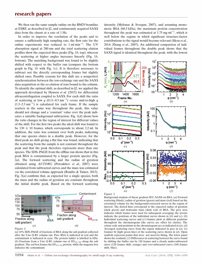
Figure 1Linear gradient IEC–SAXS performed on BSA. (a) Standard ion-exchange chromatogram of BSA on the Uno Q-1R column, highlightingthe locations of the three peaks. Orange line, percentage of buffer B; redline, resulting conductivity; violet line, absorbance at 280 nm. (b) IEC–SAXS chromatograms of BSA using a linear salt gradient. Top panel, UVabsorbance (violet) and total scattering intensity (green). Middle andbottom panels, chromatograms of sample (red) and buffer (black) runs atq = 1 nm�1 (middle) and 4 nm�1 (bottom). (c) Difference between thescattering intensities measured at q = 4 nm�1 in the sample and bufferruns (blue symbols). The dotted orange line illustrates the salt gradient.(d) Comparison of the scattering ratio (0.11–0.5 nm�1 versus 1.5–2.5 nm�1) for background correction using a shift of 100 frames (cyan),130 frames (blue) and 160 frames (green) between the sample and bufferruns. The dotted black line serves as a visual aid for a constant line.

We then ran the same sample online on the BM29 beamline

at ESRF, as described in x2, and continuously acquired SAXS

data from the eluent at a rate of 1 Hz.

In order to improve the resolution of the peaks and to

ensure a sufficiently high sampling rate, the flow rate for the

online experiments was reduced to 1 ml min�1. The UV

absorption signal at 280 nm and the total scattering elution

profiles show the expected three peaks (Fig. 1b, top), whereas

the scattering at higher angles increases linearly (Fig. 1b,

bottom). The matching background was found to be slightly

shifted with respect to the buffer run (compare the bottom

graph in Fig. 1b with Fig. 1c). It is therefore necessary to

subtract not the directly corresponding frames but slightly

shifted ones. Possible reasons for this shift are a nonperfect

synchronization between the ion-exchange run and the SAXS

data acquisition or the co-elution of ions bound to the column.

To identify the optimal shift, as described in x2, we applied the

approach developed by Hynson et al. (2015) for differential

ultracentrifugation coupled to SAXS. For each shift the ratio

of scattering at low q (0.11–0.5 nm�1) versus mid-to-high q

(1.5–2.5 nm�1) is calculated for each frame. If the sample

scatters in the same way throughout the peak, this value

should not change and a ‘constant’ value over the peak indi-

cates a suitable background subtraction. Fig. 1(d) shows how

the ratio changes in the region of interest for different values

of the shift. For the first two peaks the ideal shift was found to

be 130 � 10 frames, which corresponds to about 2.2 ml. In

addition, the ratio was constant over both peaks, indicating

that one species elutes in a double peak. However, for the

third peak no shift giving a flat line was found, indicating that

the scattering from the sample is not constant throughout the

peak and that the peak therefore represents more than one

species. The SDS–PAGE from the offline run shows that in this

peak BSA is contaminated by a larger protein species (Fig.

2a). The forward scattering and the radius of gyration

obtained using AUTORG (Petoukhov et al., 2007) were

calculated from subtracted curves and the mass was estimated

via the correlated volume approach (Rambo & Tainer, 2013).

Fig. 3(a) confirms that, as expected for a single species, both

the mass and the radius of gyration are constant throughout

the initial double peak. Based on the forward scattering

intensity (Mylonas & Svergun, 2007), and assuming mono-

meric BSA (66.5 kDa), the maximum protein concentration

throughout the peak was estimated at 1.75 mg ml�1, which is

well below the regime in which significant structure-factor

contributions to the signal would become relevant (Skou et al.,

2014; Zhang et al., 2007). An additional comparison of indi-

vidual frames throughout the double peak shows that the

SAXS signal is identical throughout the peak, with the lowest

research papers

1094 Hutin et al. � Online ion-exchange chromatography for small-angle X-ray scattering Acta Cryst. (2016). D72, 1090–1099

Figure 2(a) 10% SDS–PAGE of fractions of BSA along the salt gradient collectedafter the Uno Q-R1 column run. Pure BSA is indicated in teal and thecontaminant is indicated in cyan. The protein ladder is labelled in kDa.(b) Fractions from a Uno Q-R1 column run of D5323–785 along the saltgradient. The red box frames the D5323–785 protein, while the magenta boxindicates the contaminant.

Figure 3Background analysis of linear gradient IEC–SAXS on BSA. (a) Forwardscattering (black), radius of gyration (green) and mass (red) based on thecorrelated volume for the background-corrected curves in the region ofinterest. The dotted lines correspond to the expected radius of gyration(dark green) and molecular mass (dark red) of BSA. The grey areaindicates which frames were used for subsequent averaging; the arrowsindicate the positions of the individual curves shown in (b) and (c). (b)Individual scattering curves and (c) Guinier plots at different positionsthroughout the chromatogram (the curves are offset for clarity). Thecolour code and positions in the chromatogram are as indicated in (a). (d)Averaged scattering curve from the region indicated in grey in (a). (e)Guinier fit (light green line) of the scattering curve shown in (d). Opensymbols represent points that were not used for fitting. The lower panelshows the residuals. ( f ) Differences in scattering between the curve foundby shifting the buffer run by 130 frames and a clearly under-subtractedcurve (120 frames shift, orange) and over-subtracted curve (160 framesshift, blue).

adjusted p-value in a CORMAP test (Franke et al., 2015) being

0.16 (Figs. 3b and 3c). This suggests that the two subpeaks do

not represent different conformations of BSA. 169 frames

were averaged in the region of interest shown (grey) in Fig.

3(a). The resulting curve (Fig. 3d) gives a radius of gyration of

2.7 � 0.1 nm (Fig. 3e) and a Porod volume of 116 � 5 nm3,

corresponding to a molecular weight of about 68 kDa

(Petoukhov et al., 2007; see Table 1 for further details). Both of

these values correspond well to the expected size (2.77 nm;

PDB entry 3v03; Majorek et al., 2012) and molecular weight

(66.5 kDa) of monomeric BSA. Additional comparison to the

monomeric crystal structure (PDB entry 3v03; Majorek et al.,

2012) shows a similarly good match as the SEC–SAXS data for

BSA (�2 = 1.82; Fig. 5d and Supplementary Fig. S1b). To

estimate to what extent an incorrect shift affects these results,

the corresponding averages for shifts of 120 and 140 frames,

respectively, were calculated. The absolute differences from

the 130-frame shift are shown in Fig. 3( f). In both cases, above

1 nm�1 the curve is shifted by a small constant, which many

modelling algorithms take into account (Knight & Hub, 2015;

Petoukhov et al., 2007; Svergun et al., 1995). Below 1 nm�1

differences in the relative contribution of capillary scattering

result in a q-dependent difference, which could in principle

affect modelling. However, these differences contribute less

than 0.2% to the scattering signal and thus their influence is

negligible.

3.2. IEC–SAXS of bovine serum albumin using a stepwise saltgradient

The linear gradient IEC works well for many proteins, but

for samples where the elution peak is broad or is not well

separated from other peaks, manual selection of appropriate

steps in the gradient can ensure a purer and higher peak on

faster timescales. For these cases, we describe an elution

system in which the salt concentration is increased in prede-

fined steps. The advantage of this approach is that by choosing

a sufficiently long step length, it is possible to use buffer

measurements from the same chromatography run for back-

ground correction, reducing the risk of nonmatching buffers

owing to slow drifts. On the downside, even if the change in

the buffer mixing ratio at the pumps is instantaneous, various

effects, such as Taylor dispersion of flow in the capillary (see,

for example, Wunderlich et al., 2014), co-elution of small

molecules from the columns and the creation of new inter-

action sites for salt on the column and the eluted protein,

result in non-instantaneous gradients at the measurement

position. To show the validity of this approach, we again used

BSA with the salt concentrations determined above from the

offline IEC run.

The elution steps were chosen in such a way that the first

two subpeaks of the BSA elute in the same step. In this case,

BSA elutes as a single peak (Fig. 4a). As expected, the

background scattering at high angles does not increase

instantaneously, but saturates slowly after a steep initial

increase. In order to subtract an appropriate background from

each measured frame, it is necessary to interpolate between

the two buffers recorded before and after the peak. As the

scattering of BSA at high angles is rather low and the increase

in signal above q = 4.5 nm�1 does not follow the protein

concentration (Fig. 4a), one can assume that the changes in

signal in this region are only owing to the difference in

background. In order to limit the effect of the rather high

noise level in this region, the increase is modelled with a

research papers

Acta Cryst. (2016). D72, 1090–1099 Hutin et al. � Online ion-exchange chromatography for small-angle X-ray scattering 1095

Figure 4Stepwise-gradient IEC–SAXS performed on BSA. (a) IEC–SAXSchromatograms of BSA using a stepwise salt gradient. Top panel, UVabsorbance (violet) and total scattering intensity (green). Middle andbottom panels, chromatograms at 1 and 4 nm�1, respectively. (b) Thebuffer signal (mean scattering above 4.5 nm�1, blue) increases slowlyduring the elution of the peak (total scattering intensity, green) and canbe modelled by an exponential decay (red) between the buffer before thepeak (I) and after the peak (II). (c) Comparison of the scattering ratio(0.11–0.5 nm�1 versus 1.5–2.5 nm�1) for background correction using thebuffer before the peak (I, cyan), after the peak (II, green) and themodelled buffer (blue). (d) Forward scattering (black), radius of gyration(green) and mass (red) based on the correlated volume for thebackground-corrected curves in the peak region. The grey area indicatesthe frames that were used for subsequent averaging; the arrows indicatethe positions of the individual curves presented in (e) and ( f ). (e)Individual scattering curves and ( f ) Guinier plots at different positionsthroughout the chromatogram (curves are offset for clarity). The colourcode and the positions in the chromatogram are as indicated in (d).

continuous function instead of using the high-q region of each

frame to interpolate the buffer individually. A least-parameter

model for an asymmetric, saturating increase as observed here

is a single exponential decay from the buffer before (region I)

to the buffer after (region II) the peak, i.e. a fit to II � (II �

I)exp[�(N � N0)/N0], where N is the frame number, N0 is a

constant offset and 1/N0 is the rate of increase. To obtain the

correct values for N0 and N0, the mean of the data was fitted

above 4.5 nm�1 (Fig. 4b). The best fit is obtained with N0 =

1289 � 2 and N0 = 17 � 3, giving an �2 of 0.86. These para-

meters match the starting point of the increase (frame 1290)

and the estimated half-life of 12 � 2 frames well and allow us

to model the entire q-range.

This procedure allows the background to be subtracted

individually for each frame and a constant scattering from the

sample throughout the peak to be confirmed by assessing the

stability of the ratio of scattering at low q versus mid/high q, as

discussed above (Figs. 4c and 4d). Individual comparison of

frames confirmed this constant signal (Figs. 4e and 4f). Based

on the forward scattering, the maximum concentration in this

case was only 0.35 mg ml�1. After averaging (Fig. 5a), a scat-

tering curve which corresponds to monomeric BSA (�2 = 3.63;

Fig. 5d) was found. The radius of gyration is 2.7 � 0.1 nm

(Fig. 5b) and the Porod volume is 116 � 5 nm3, matching

previous results (also see Table 1). This shows that important

structural parameters can be determined using either linear or

stepwise gradients.

In order to estimate the mis-subtraction of the buffer and its

effect on the conclusions that can be drawn from the data, one

needs to determine corresponding over-subtracted and under-

subtracted curves. We decided to over-subtract by directly

subtracting buffer II and to under-subtract by subtracting the

mean of buffer I and buffer II. This choice might be more

extreme than strictly necessary, but provides an upper limit of

the effect of the mis-subtraction. The differences in this case

(Fig. 5c) are much more pronounced than for a linear gradient

case (Fig. 3f). This means that the background subtraction for

the linear case is more accurate.

Above 1 nm�1, buffer mismatch causes a constant shift in

the signal. Below 1 nm�1, the differences are larger but do not

impact the structural parameters determined from this region,

with the radius of gyration remaining at 2.7 � 0.1 nm and the

Porod volume increasing within its error to 120 � 5 nm3 only

for the subtraction of buffer II and remaining unchanged for

the other case.

This implies that while interpretations of domain arrange-

ments might be affected by buffer mismatches, the observed

overall shape (size, anisotropy, . . . ) of the protein can still be

determined despite the larger inaccuracy in the background

subtraction.

Direct comparison of the two scattering curves of BSA

obtained using the two different IEC–SAXS approaches

(Fig. 5d) shows two very similar curves. Owing to the lower

protein concentration at the peak, the curve resulting from the

step-gradient method is noisier. However, from about

2.5 nm�1 onwards the signal determined using the linear

gradient method decreases more steeply. In particular, above

3.5 nm�1 the signal determined using the step gradient turns

upward. This increase also results in a clear deviation from the

predicted signal and is responsible for the higher �2.

3.3. IEC–SAXS of the helicase–primase protein D5323–785using a stepwise salt gradient

To demonstrate the applicability of this approach to a novel

sample, we selected D5323–785, the D5N and helicase domains

of the Vaccinia virus helicase–primase D5. The protein frag-

ment forms a hexamer (320.88 kDa) that is required for its

activity (Hutin et al., 2016). After two nickel columns and

a size-exclusion chromatography step, a contaminant still

persisted and required an additional purification step via ion-

exchange chromatography (Fig. 2b), followed by an additional

size-exclusion chromatography step. Each step takes time and

about 30–50% of the material is lost in total. To optimize the

data-collection strategy it would be advantageous to measure

the hexamer directly from the Uno Q-1R column.

In the standard offline IEC experiment using a linear

gradient, three not completely separated peaks at 11, 14 and

16% high-salt buffer were observed (Fig. 6a).

When using a stepwise gradient a sharp peak is obtained

(Fig. 6b) at 12% salt buffer (142 mM NaCl) and small addi-

research papers

1096 Hutin et al. � Online ion-exchange chromatography for small-angle X-ray scattering Acta Cryst. (2016). D72, 1090–1099

Figure 5Stepwise-gradient IEC–SAXS analysis of averaged BSA data. (a)Scattering curve based on averaging of the region indicated in grey inFig. 4(d). (b) Guinier fit (light blue line) of the scattering curve shown in(a). Open symbols represent points that were not used for fitting. Thelower panel shows the residuals. (c) Differences in scattering between thecurve found by interpolating the buffer and a clearly under-subtractedcurve (average of buffers from regions I and II, orange) and over-subtracted curve (buffer from region II, blue). (d) Fits to the monomericcrystal structure of BSA (PDB entry 3v03; Majorek et al., 2012) elutedwith a linear gradient (green) and a stepwise gradient (blue).

tional peaks in the subsequent steps. This indicates that

D5323–785 elutes completely at 142 mM NaCl and the peaks are

better separated than in the linear-gradient elution procedure

(Fig. 2a). The scattering at high q (4 nm�1) slightly overshoots

the scattering level expected from the buffer run (Fig. 6c),

probably owing to the co-elution of small ions. To check that

the sample composition does not change throughout the peak,

the low-salt buffer from each frame was subtracted and their

radii of gyration were compared. This operation is not affected

by the small change of background throughout the peak (data

not shown). Based on the forward scattering from this preli-

minary processing, the maximum protein concentration is

estimated to be 3.4 mg ml�1, corresponding to a 20-fold

increase from the injected concentration of 0.17 mg ml�1.

Owing to the irregular changes in the background signal

that were observed in these data, the approaches to modelling

the change in background signal on a frame-by-frame basis

that were applied to the previous examples are not applicable.

To overcome this issue, first the frames in the peak were

averaged in order to improve the signal-to-noise ratio in the

high-q region, and a matching buffer from a salt-concentration

series measured directly before the ion-exchange run was then

chosen by comparing the average scattering in the q-range

between 4.25 and 4.75 nm�1.

The resulting curve (Fig. 7a) has a radius of gyration of

4.7 nm (Fig. 7b) and a Porod volume of 577 � 5 nm3, corre-

sponding to a mass of 338 kDa (Petoukhov et al., 2007),

matching the hexamer mass of 320 kDa well (see also Table 1).

The P(r) function (Fig. 7c) shows one peak that is slightly

shifted to larger distances. This shape, in addition to the clear

minima, hints at a mostly spherical shape with a cavity and

matches the expected molecular shape well (Hutin et al.,

2016).

As the steps were chosen more finely than in the previous

experiment with BSA, it is easier to estimate the degree of

buffer mismatch in the D5323–785 experiment. The extent to

which it influences the interpretation of the results can be

estimated by selecting buffers from a higher and a lower salt

step of the buffer run (Fig. 7d). In both cases the resulting

curve is distinguished from the reported curve by a small

constant above q = 0.8 nm�1. Below q = 0.8 nm�1 the devia-

tions are no longer constant but are below 0.1% of the signal,

and therefore do not influence the interpretation.

3.4. Additional considerations

One of the major difficulties in online SEC–SAXS is the

effect of radiation damage on the observed signal. The

continuously changing signal makes assessment of radiation-

research papers

Acta Cryst. (2016). D72, 1090–1099 Hutin et al. � Online ion-exchange chromatography for small-angle X-ray scattering 1097

Figure 6IEC–SAXS of D5323–785. (a) Ion-exchange chromatogram of D5323–785 onthe Uno Q-1R column with the three peaks indicated. Orange line,percentage of buffer B; red line, the resulting conductivity; violet line,absorbance at 280 nm. (b) IEC–SAXS chromatograms of D5323–785 usinga stepwise salt gradient. Top panel, UV absorbance (violet) and totalscattering intensity (green). Middle and bottom panels, chromatograms ofsample (red) and buffer (black) runs at q = 1 nm�1 (middle) and 4 nm�1

(bottom). (c) Enlargement of the lower panel in (b): in the protein run(red) the signal at high q overshoots in comparison to the buffer run.

Figure 7(a) Average sample (violet) and buffer (black) curves for the D5323–785

protein, the resulting subtraction (red) and the fit for calculating the P(r)function (blue). (b) Guinier fit (black line) of the scattering curve shownin (a). Open symbols represent points that were not used for fitting. Thelower panel shows the residuals. (c) Pair distance distribution function ofthe average curve, showing a single peak. (d) Differences in scatteringbetween the curve based on the best-matching buffer and a clearly under-subtracted curve (preceding buffer step, orange) and over-subtractedcurve (subsequent buffer step, blue).

induced changes to the SAXS signal difficult. In addition,

radiation-damaged material often displays a tendency to

adhere to the surfaces of the sample environment (Brookes et

al., 2013; Jeffries et al., 2015). IEC–SAXS can be performed at

relatively high flow rates (1 ml min�1 for the studies in this

publication); consequently, the average dwelling time of

material in the X-ray beam is shorter than for standard SEC–

SAXS experiments and the contribution of damaged material

to the signal is reduced. Furthermore, the higher flow rate

reduces the risk of damaged material spoiling the sample

environment by adhering to the surface (Epstein, 1997).

4. Conclusions

For many macromolecules in solution, ion-exchange chroma-

tography is a required step and is the best-suited purification

method, as it can often separate similarly sized proteins.

However, the IEC step is usually followed by another purifi-

cation step, or dialysis, to ensure optimal buffer subtraction.

Here, we demonstrate for the first time the application of ion-

exchange chromatography directly prior to SAXS measure-

ments.

The linear gradient method presented here is analogous to

a standard ion-exchange protocol and does not inherently

require additional offline tests. In addition, background

correction can be achieved by correct alignment of a buffer

run without any need for interpolation. As each frame can be

corrected individually, it is possible to confirm a stable signal

throughout the peak. However, owing to the continuity of the

gradient, sharp and well separated peaks are beneficial.

By carefully selecting the salt concentration of the steps in

the step-elution method, this method allows the separation of

the peaks to be improved, as no limit exists on the number of

substeps. However, background subtraction requires more

caution, as the discontinuity of the elution gradient results in

the discontinuous co-elution of small ions. In our first example

(BSA), it was still possible to correct the background indivi-

dually for each frame by interpolating the buffer signal. In our

second example (D5323–785) it was not possible to interpolate

the background throughout the peak, and the correction by

framewise comparisons was not applicable. Nevertheless, the

correct background for the average signal can be found by

measuring a variety of mixing ratios prior to the experiment

and carefully choosing the matching one. Despite this diffi-

culty, we are confident that it can be applied to a wide variety

of biological macromolecules.

Online ion-exchange chromatography adds another

important biochemical purification method to the repertoire

of purification methods which can be coupled with SAXS

(Round et al., 2013; David & Perez, 2009; Graewert et al., 2015;

Jensen et al., 2010; Hynson et al., 2015; Mathew et al., 2004;

Watanabe & Inoko, 2009). Proteins of similar apparent

molecular weight, but different net surface charges, can now

be separated online using the IEC–SAXS method. While

background subtraction is slightly less straightforward than for

SEC–SAXS, the variation in the background is smaller than

for differential ultracentrifugation coupled with SAXS owing

to the high sugar content of the latter (from 15 to 35% sucrose;

Hynson et al., 2015). The background-correction method here

for D5323–785, based on averages, can be performed using any

software package for SAXS data analysis, such as PRIMUS

(Konarev et al., 2003) or SCATTER, assuming that the

possible buffer range has been well determined experimen-

tally.

For IEC, buffer conditions, such as salt concentrations or

pH, are primarily determined by the biochemical character-

istics of the protein of interest, such as its isoelectric point and

solubility (Yigzaw et al., 2009). However, one should aim to

minimize the amounts of all additives in order to maximize the

X-ray contrast between the protein and the buffer in a SAXS

experiment.

As with any SAS data, IEC–SAXS results need to be

carefully validated. Special care should be paid to sample

monodispersity, which cannot be directly assessed by IEC–

SAXS, and correct background subtraction, especially in the

case of flexible proteins (Jacques et al., 2012; Jacques &

Trewhella, 2010). It is important to estimate how mis-

subtraction would affect the conclusions drawn from the data.

For the results shown in this paper, we have shown that

deviations from the ideal background subtraction are small

enough to allow reliable conclusions.

In conclusion, IEC–SAXS is a useful technique that allows

accurate data collection with fewer preparation steps and

minimizing the loss of time and sample. Proof of principle of a

simple elution method is demonstrated in this paper with the

option to optimize species separation by using steps in the salt

gradient. Validation of three different approaches to achieve

optimal background subtractions is also given. A suitable

combination of elution method and background subtraction

can be chosen to suit the sample of interest best and to provide

necessary information for data validation (as demonstrated),

so that the resulting data can be used with confidence for

subsequent analysis and modelling using the standard tools

available within the scientific community.

The online SEC system installed at BM29 can routinely

perform these experiments and is available for user access on

request.

Acknowledgements

We thank the ESRF for SAXS beam time and support. We

further wish to acknowledge Wim Burmeister from Universite

Grenoble Alpes for fruitful discussions and financial support.

This work was supported by an ANR grant (REPLIPOX,

ANR-13-BSV8-0014). We would like to thank Petra Pernot

and Matthew Bowler for proofreading the manuscript.

References

Acerbo, A. S., Cook, M. J. & Gillilan, R. E. (2015). J. SynchrotronRad. 22, 180–186.

Ashiotis, G., Deschildre, A., Nawaz, Z., Wright, J. P., Karkoulis, D.,Picca, F. E. & Kieffer, J. (2015). J. Appl. Cryst. 48, 510–519.

Brennich, M. E., Kieffer, J., Bonamis, G., De Maria Antolinos, A.,Hutin, S., Pernot, P. & Round, A. (2016). J. Appl. Cryst. 49,203–212.

research papers

1098 Hutin et al. � Online ion-exchange chromatography for small-angle X-ray scattering Acta Cryst. (2016). D72, 1090–1099

Brookes, E., Perez, J., Cardinali, B., Profumo, A., Vachette, P. &Rocco, M. (2013). J. Appl. Cryst. 46, 1823–1833.

David, G. & Perez, J. (2009). J. Appl. Cryst. 42, 892–900.De Maria Antolinos, A., Pernot, P., Brennich, M. E., Kieffer, J.,

Bowler, M. W., Delageniere, S., Ohlsson, S., Malbet Monaco, S.,Ashton, A., Franke, D., Svergun, D., McSweeney, S., Gordon, E. &Round, A. (2015). Acta Cryst. D71, 76–85.

Epstein, N. (1997). Exp. Therm. Fluid Sci. 14, 323–334.Folta-Stogniew, E. & Williams, K. (1999). J. Biomol. Tech. 10, 51–63.Franke, D., Jeffries, C. M. & Svergun, D. I. (2015). Nature Methods,

12, 419–422.Graewert, M. A., Franke, D., Jeffries, C. M., Blanchet, C. E., Ruskule,

D., Kuhle, K., Flieger, A., Schafer, B., Tartsch, B., Meijers, R. &Svergun, D. I. (2015). Sci. Rep. 5, 10734.

Graewert, M. A. & Svergun, D. I. (2013). Curr. Opin. Struct. Biol. 23,748–754.

Grant, T. D., Luft, J. R., Wolfley, J. R., Tsuruta, H., Martel, A.,Montelione, G. T. & Snell, E. H. (2011). Biopolymers, 95, 517–530.

Hutin, S., Ling, W. L., Round, A., Effantin, G., Reich, S., Iseni, F.,Tarbouriech, N., Schoehn, G. & Burmeister, W. P. (2016). J. Virol.90, 4604–4613.

Hynson, R. M. G., Duff, A. P., Kirby, N., Mudie, S. & Lee, L. K. (2015).J. Appl. Cryst. 48, 769–775.

Jacques, D. A., Guss, J. M., Svergun, D. I. & Trewhella, J. (2012). ActaCryst. D68, 620–626.

Jacques, D. A. & Trewhella, J. (2010). Protein Sci. 19, 642–657.Jeffries, C. M., Graewert, M. A., Svergun, D. I. & Blanchet, C. E.

(2015). J. Synchrotron Rad. 22, 273–279.Jensen, M. H., Toft, K. N., David, G., Havelund, S., Perez, J. &

Vestergaard, B. (2010). J. Synchrotron Rad. 17, 769–773.Jones, E., Oliphant, T. E. & Peterson, P. (2001). SciPy: Open Source

Scientific Tools for Python. http://www.scipy.org/.Karlsson, E. & Hirsh, I. (2011). Methods Biochem. Anal. 54, 93–133.Kieffer, J. & Karkoulis, D. (2013). J. Phys. Conf. Ser. 425, 202012.Kieffer, J. & Wright, J. (2013). Powder Diffr. 28, S339–S350.Kikhney, A. G. & Svergun, D. I. (2015). FEBS Lett. 589, 2570–

2577.Kirby, N., Mudie, S., Hawley, A., Mertens, H. D. T., Cowieson, N.,

Samardzic Boban, V., Felzmann, U., Mudie, N., Dwyer, J., Beckham,S., Wilce, M., Huang, J., Sinclair, J. & Moll, A. (2013). Trans. Am.Crystallogr. Assoc. 44, 3. http://www.amercrystalassn.org/documents/2013 Transactions/3-Kirby.pdf.

Kluters, S., Wittkopp, F., Johnck, M. & Frech, C. (2015). J. Sep. Sci. 39,663–675.

Knight, C. J. & Hub, J. S. (2015). Nucleic Acids Res. 43, W225–W230.Konarev, P. V., Volkov, V. V., Sokolova, A. V., Koch, M. H. J. &

Svergun, D. I. (2003). J. Appl. Cryst. 36, 1277–1282.Lambright, D., Malaby, A. W., Kathuria, S. V., Nobrega, R. P., Bilsel,

O., Matthews, C. R., Muthurajan, U., Luger, K., Chopra, R. &Irving, T. C. (2013). Trans. Am. Crystallogr. Assoc. 44, 1.http://www.amercrystalassn.org/documents/2013 Transactions/1-Chakravarthy.pdf.

Majorek, K. A., Porebski, P. J., Dayal, A., Zimmerman, M. D.,Jablonska, K., Stewart, A. J., Chruszcz, M. & Minor, W. (2012). Mol.Immunol. 52, 174–182.

Mathew, E., Mirza, A. & Menhart, N. (2004). J. Synchrotron Rad. 11,314–318.

Mylonas, E. & Svergun, D. I. (2007). J. Appl. Cryst. 40, s245–s249.Orthaber, D., Bergmann, A. & Glatter, O. (2000). J. Appl. Cryst. 33,

218–225.Pernot, P. et al. (2013). J. Synchrotron Rad. 20, 660–664.Petoukhov, M. V., Konarev, P. V., Kikhney, A. G. & Svergun, D. I.

(2007). J. Appl. Cryst. 40, s223–s228.Putnam, C. D., Hammel, M., Hura, G. L. & Tainer, J. A. (2007). Q.

Rev. Biophys. 40, 191–285.Rambo, R. P. & Tainer, J. A. (2013). Nature (London), 496, 477–481.Round, A., Brown, E., Marcellin, R., Kapp, U., Westfall, C. S., Jez,

J. M. & Zubieta, C. (2013). Acta Cryst. D69, 2072–2080.Round, A., Felisaz, F., Fodinger, L., Gobbo, A., Huet, J., Villard, C.,

Blanchet, C. E., Pernot, P., McSweeney, S., Roessle, M., Svergun,D. I. & Cipriani, F. (2015). Acta Cryst. D71, 67–75.

Selkirk, C. (2004). Methods Mol. Biol. 244, 125–131.Skou, S., Gillilan, R. E. & Ando, N. (2014). Nature Protoc. 9, 1727–

1739.Svergun, D. I. (1992). J. Appl. Cryst. 25, 495–503.Svergun, D., Barberato, C. & Koch, M. H. J. (1995). J. Appl. Cryst. 28,

768–773.Watanabe, Y. & Inoko, Y. (2009). J. Chromatogr. A, 1216, 7461–7465.Wunderlich, B., Nettels, D. & Schuler, B. (2014). Lab Chip, 14,

219–228.Yigzaw, Y., Hinckley, P., Hewig, A. & Vedantham, G. (2009). Curr.

Pharm. Biotechnol. 10, 421–426.Zhang, F., Skoda, M. W., Jacobs, R. M., Martin, R. A., Martin, C. M. &

Schreiber, F. (2007). J. Phys. Chem. B, 111, 251–259.

research papers

Acta Cryst. (2016). D72, 1090–1099 Hutin et al. � Online ion-exchange chromatography for small-angle X-ray scattering 1099