Online Appendix toProductivity and Misallocation in General

Equilibrium

David Rezza Baqaee Emmanuel Farhi

March 10, 2020

∗Emails: baqaee@econ.ucla.edu, efarhi@harvard.edu. We thank Philippe Aghion, Pol Antras, AndrewAtkeson, Susanto Basu, John Geanakoplos, Ben Golub, Gita Gopinath, Dale Jorgenson, Marc Melitz, BenMoll, Matthew Shapiro, Dan Trefler, Venky Venkateswaran and Jaume Ventura for their valuable comments.We are especially grateful to Natalie Bau for detailed conversations. We thank German Gutierrez, ThomasPhilippon, Jan De Loecker, and Jan Eeckhout for sharing their data. We thank Thomas Brzustowski andMaria Voronina for excellent research assistance.

55

B Empirical Comparison with Petrin-Levinsohn 57

C Data 58C.1 Input-Output and Aggregate Data . . . . . . . . . . . . . . . . . . . . . . . . 58C.2 Estimates of Markups . . . . . . . . . . . . . . . . . . . . . . . . . . . . . . . . 59

D Proofs 62

E Basu-Fernald and Petrin-Levinsohn in a Simple Example 69

F Applying our Results with Endogenous Markups in a Simple Example 70

G Standard-Form for Nested CES Economies 72

H Robustness and Extensions 73H.1 Beyond CES . . . . . . . . . . . . . . . . . . . . . . . . . . . . . . . . . . . . . 73H.2 Elastic Factor Supplies . . . . . . . . . . . . . . . . . . . . . . . . . . . . . . . 74H.3 Capital Accumulation, Adjustment Costs, and Capacity Utilization . . . . . 76H.4 Nonlinear Impact of Shocks and Duality with Industry Structure . . . . . . 76

I Aggregation of Cost-Based Domar Weights 80

J Extra Examples 81

K Volatility of Aggregate TFP 84

56

Appendix B Empirical Comparison with Petrin-Levinsohn

Figure 8 constructs the Petrin-Levinsohn decomposition with markups obtained from theproduction-function approach, at the firm level. The factor-growth-miscounting term isintroduced to correct for the fact that the Petrin-Levinsohn decomposition applies to theSolow residual, whereas ours applies to the distortion-adjusted Solow residual, whereboth residuals weigh the growth of each factor differently. It does not affect the puretechnology and changes in allocative efficiency effects constructed using their procedure.

Figures 6a and 8 allow us to compare the different results that are obtained using ourdecomposition and the Petrin-Levinsohn decomposition. Compared to ours, the Petrin-Levinsohn decomposition finds lower contributions both for pure technology and forallocative efficiency. The different weights used to weigh labor and capital growth in theSolow residual vs. the distortion-adjusted Solow also lead to a sizable difference betweenthe Solow residual and the distortion-adjusted Solow residual. The cumulated Solowresidual is significantly lower than the cumulated distortion-adjusted Solow residual, andthis is reflected in a sizable positive contribution of factor-growth miscounting.

1996 1998 2000 2002 2004 2006 2008 2010 2012 2014

−0.10

0.00

0.10

0.20

Distorted Solow ResidualAllocative Efficiency a la PLTechnology a la PLReweighting of Factor Growth

Figure 8: Petrin-Levinsohn decomposition of changes in aggregate TFP into pure changesin technology, changes in allocative efficiency, and factor under-counting, with markupsobtained from the production-function approach, at the firm level.

57

Appendix C Data

We have two principal datasources: (i) aggregate data from the BEA, including the input-output tables and the national income and product accounts; (ii) firm-level data fromCompustat. Below we describe how we treat the input-output data, merge it with firm-level estimates of markups, and how we estimate markups at the firm-level.

C.1 Input-Output and Aggregate Data

Our measure of real GDP growth, and growth in real factor quantities (labor and capi-tal) come from the San Francisco Federal Reserve’s dataset on total factor productivity.1

Specifically, we use the variable “dY” for real GDP growth, “dK” for real capital growth,and “dLQ+dhours” for labor input growth.

Our input-output data comes from the BEA’s annual input-output tables. We calibratethe data to the use tables from 1997-2015 before redefinitions. We also ignore the dis-tinction between commodities and industries, assuming that each industry produces onecommodity. For each year, this gives us the revenue-based expenditure share matrix Ω aswell as the final demand budget shares b. We drop the government, scrap, and noncom-parable imports sectors from our dataset, leaving us with 66 industries. We define thegross-operating surplus of each industry to be the residual from sales minus intermediateinput costs and compensation of employees. The expenditures on capital, at the industrylevel, are equal to the gross operating surplus minus the share of profits (how we calculatethe profit share is described shortly). If this number is negative, we set it equal to zero. Ifany value in Ω is negative, we set it to zero.

We have three sources of markup data. For each markup series, we compute the profitshare (amongst Compustat firms) for each industry and year, and then we use that profitshare to separate payments to capital from gross operating surplus in the BEA data for thatindustry and year. Conditional on the harmonic average of markups in each industry-year, we can recover the cost-based Ω = µΩ. If for an industry and year we do not observeany Compustat firms, then we assume that the profit share (and the average markup) ofthat industry is equal to the aggregate profit share (and the industry-level markup is thesame as the aggregate markup).

We assume that the economy has an industry structure along the lines of AppendixH.4, so that all producers in each industry have the same production function up to aHicks-neutral productivity shifter. This means that for each producer i and j in the same

1Available at https://www.frbsf.org/economic-research/indicators-data/total-factor-productivity-tfp/

58

industry Ωik = Ω jk. To populate each industry with individual firms, we divide the salesof each industry across the firms in Compustat according to the sales share of these firmsin Compustat. In other words, if some firm i’s markup is µi and share of industry sales inCompustat is x, then we assume that the mass of firms in that industry whose markupsare equal to µi is also equal to x. These assumptions allow us to use the markup dataand market share information from Compustat, and the industry-level IO matrix from theBEA, to construct the firm-level cost-based IO matrix.

C.2 Estimates of Markups

Now, we briefly describe how our firm-level markup data is constructed. Firm-leveldata is from Compustat, which includes all public firms in the U.S. The database covers1950 to 2016, but we restrict ourselves to post-1997 data since that is the start of theannual BEA data. We exclude firm-year observations with assets less than 10 million,with negative book or market value, or with missing year, assets, or book liabilities. Weexclude firms with BEA code 999 because there is no BEA depreciation available for them;and Financials (SIC codes 6000-6999 or NAICS3 codes 520-525). Firms are mapped toBEA industry segments using ‘Level 3’ NAICS codes, according to the correspondencetables provided by the BEA. When NAICS codes are not available, firms are mapped tothe most common NAICS category among those firms that share the same SIC code andhave NAICS codes available.

C.2.1 Accounting Profits Approach

For the accounting-profit approach markups, we use operating income before deprecia-tion, minus depreciation to arrive at accounting profits. Our measure of depreciation is theindustry-level depreciation rate from the BEA’s investment series. The BEA depreciationrates are better than the Compustat depreciation measures since accounting rules and taxincentives incentivize firms to depreciate assets too quickly. We use the expression

pro f itsi =

(1 −

1µi

)salesi,

to back out the markups for each firm in each year. We winsorize markups and changesin markups at the 5-95th percentile by year. Intuitively, this is equivalent to assuming thatthe cost of capital is simply the depreciation rate (equivalently, the risk-adjusted rate ofreturn on capital is zero).

59

C.2.2 User Cost Approach

The user-cost approach markups are similar to the accounting profits but require a morecareful accounting for the user cost of capital. For this measure, we rely on the replicationfiles from Gutierrez and Philippon (2016) provided German Gutierrez. For more informa-tion see Gutierrez and Philippon (2016). To recover markups, we assume that operatingsurplus of each firm is equal to payments to both capital as well as economic rents due tomarkups. We write

OSi,t = rki,tKi,t +

(1 −

1µi

)salesi,t,

where OSi,t is the operating income of the firm after depreciation and minus income taxes,rki,t is the user-cost of capital and Ki,t is the quantity of capital used by firm i in industryj in period t. This equation uses the fact that each firm has constant-returns to scale. Inother words,

OSi,t

Ki,t= rki,t +

(1 −

1µi

)salesi,t

Ki,t, (21)

To solve for the markup, we need to account for both the user cost (rental rate) of capitalas well as the quantity of capital. The user-cost of capital is given by

rki,t = rst + KRP j − (1 − δki,t)E(Πk

t+1),

where rst is the risk-free real rate, KPR j is the industry-level capital risk premium, δ j is the

industry-level BEA depreciation rate, and E(Πkt+1) is the expected growth in the relative

price of capital. We assume that expected quantities are equal to the realized ones. Tocalculate the user-cost, the risk-free real rate is the yield on 10-year TIPS starting in 2003.Prior to 2003, we use the average spread between nominal and TIPS bonds to deduce thereal rate from nominal bonds prior to 2003. KRP is computed using industry-level equityrisk premia following Claus and Thomas (2001) using analyst forecasts of earnings fromIBES and using current book value and the average industry payout ratio to forecast futurebook value. The depreciation rate is taken from BEA’s industry-level depreciation rates.The capital gains E(Πk

t+1) is equal to the growth in the relative price of capital computedfrom the industry-specific investment price index relative to the PCE deflator. Finally, weuse net property, plant, and equipment as the measure of the capital stock. This allows usto solve equation (21) for a time-varying firm-level measure of the markup. We winsorizemarkups and changes in markups at the 5-95th percentile by year.

60

C.2.3 Production Function Estimation Approach

For the production function estimation approach markups, we follow the procedure PF1described by De Loecker et al. (2019) with some minor differences. We estimate theproduction function using Olley and Pakes (1996) rather than Levinsohn and Petrin (2003).We use CAPX as the instrument and COGS as a variable input. We use the classificationbased on SIC numbers instead of NAICS numbers since they are available for a largerfraction of the sample. Finally, we exclude firms with COGS-to-sales and XSGA-to-salesratios in the top and bottom 2.5% of the corresponding year-specific distributions. Aswith the other series, we use Compustat excluding all firms that did not report SIC orNAICS indicators, and all firms with missing sales or COGS. Sales and COGS are deflatedusing the gross output price indices from KLEMS sector-level data. CAPX and PPEGT –using the capital price indices from the same source. Industry classification used in theestimation is based on the 2-digit codes whenever possible, and 1-digit codes if there arefewer than 500 observations for each industry and year.

To compute the PF Markups, we need to estimate elasticity of output with respectto variable inputs. This is because once we know the output-elasticity with respect to avariable input (in this case, the cost of goods sold or COGS), then following Hall (1988),the markup is

µi =∂ log Fi/∂ log COGSi

Ωi,COGS,

where Ωi,COGS is the firm’s expenditures on COGS relative to its turnover.The output-elasticities are estimated using Olley and Pakes (1996) methodology with

the correction advocated by Ackerberg et al. (2015). To implement Olley-Pakes in Stata,we use the prodest Stata package. OP estimation requires:

(i) outcome variable: log sales,

(ii) ”free” variable (variable inputs): log COGS,

(iii) ”state” variable: log capital stock, measured as log PPEGT in the Compustat data,

(iv) ”proxy” variable, used as an instrument for productivity: log investment, measuredas log CAPX in Compustat data.

(v) in addition, SIC 3-digit and SIC 4-digit firm sales shares were used to control formarkups .

Given these data, we run the estimation procedure for every sector and every year.Since panel data are required, we use 3-year rolling windows so that the elasticity estimates

61

based on data in years t − 1, t and t + 1 are assigned to year t. The estimation procedurehas two stages: in the first stage, log sales are regressed on the 3-rd degree polynomialof state, free, proxy and control variables in order to remove the measurement error andunanticipated shocks; in the second stage, we estimate elasticities of output with respectto variable inputs and the state variable by fitting an AR(1) process for productivity tothe data (via GMM). Just like in De Loecker et al. (2019), we control for markups using alinear function of firm sales shares (sales share at the 4-digit industry level).

We use a Cobb-Douglas specification of industry production functions because of itssimplicity and stability. This means that to be entirely internally consistent, in our struc-tural counterfactual exercise regarding the effect of removing markups on aggregate TFP,we should focus on specifications with unitary elasticities across industries and factors.For example, the benchmark should now be the CD+CES specification in the second col-umn of Table 2 instead of that in the first column. Imposing elasticities across industriesand factors would only introduce minor quantitative differences as we navigate throughthe other columns, and would not change the corresponding quantitative conclusionsmuch.

Appendix D Proofs

Throughout this appendix, we let the nominal GDP be the numeraire, so that PY =∑Ni=1 pici = 1 or equivalently d log(

∑Ni=1 pici) = 0. This numeraire is different from the GDP

deflator defined such that the ideal price index of the household is unitary P = 1, orequivalently d log P =

∑Ni=1 bid log pi = 0. A price pi in the nominal GDP numeraire can

easily be converted into a price piY in the GDP deflator numeraire, so that d log(piY) =

d log pi + d log Y.

Proof of Theorem 1. We start by proving some preliminary results. Let Ωp be the N × Nmatrix corresponding to the first N rows and columns (corresponding to goods prices)of Ω, so that Ω

pij = Ω

pij for (i, j) ∈ [1,N]2. Since Ω is block-diagonal over goods prices and

factor prices, we have that for all (i, j) ∈ [1,N]2,

[(I − Ωp)−1]i j = [(I − Ω)−1]i j = Ψi j. (22)

In addition, using

1 =

N∑j=1

Ωi j +

F∑f=1

Ωi f , (23)

62

which we can rewrite as1p = Ωp1p + Ω1 f , (24)

where 1p is a N × 1 vector of ones and 1 f is a F× 1 vector of ones. This in turn implies that

1p = (I − Ωp)−1Ω1 f , (25)

and hence1p = Ψ1 f , (26)

1 = b′Ψ1 f , (27)

and finally, usingb′Ψ = λ′, (28)

we get

1 =

F∑f=1

Λ f . (29)

We now move on to the main proof. By Sheppard’s lemma, we have

d log pi = −d log Ai + d logµi +

N∑j=1

Ωi jd log p j +

F∑f=1

Ωi f d log w f . (30)

In the nominal GDP numeraire where∑

pici = 1, we have w f L f = Λ f . Since we hold factorsupplies fixed, we have

d log w f = d log Λ f . (31)

This implies that

d log pi = −d log Ai + d logµi +

N∑j=1

Ωi jd log p j +

F∑f=1

Ωi f d log Λ f . (32)

We can rewrite this as

d log pi =

N∑k=1

[(I − Ωp)−1]ik(−d log Ak + d logµk) +

F∑f=1

N∑k=1

[(I − Ωp)−1]ikΩk f d log Λ f . (33)

63

This implies that

d log pi =

N∑k=1

Ψik(−d log Ak + d logµk) +

F∑f=1

N∑k=1

ΨikΩk f d log Λ f . (34)

This in turn implies that

d log pi =

N∑k=1

Ψik(−d log Ak + d logµk) +

F∑f=1

Ψi f d log Λ f . (35)

This can be rewritten in vector form as

d log p =

N∑k=1

Ψ(k)(−d log Ak + d logµk) +

F∑f=1

Ψ( f )d log Λ f , (36)

where Ψ(k) and Ψ( f ) are the k-th and f -th columns of Ψ, respectively. Since

d log Y = −b′d log p = −

N∑i=1

bid log pi, (37)

and sinceb′Ψ = λ′, (38)

we get finally get

d log Y =

N∑k=1

λkd log Ak −

N∑k=1

λkd logµk −

F∑f=1

Λ f d log Λ f . (39)

which proves Theorem 1.

Proofs of Propositions 2 and 3. We have

dΩ ji = −Ω jid logµ j +1µ j

(θ j − 1)

d log pi −

∑l

Ω jld log pl

. (40)

or equivalently

dΩ ji = −Ω jid logµ j +1µ j

(θ j − 1)CovΩ( j)(d log p, I(i)), (41)

64

where I(i) is the ith column of the identity matrix I. Using

d log p = −∑

k

Ψ(k)d log Ak +∑

k

Ψ(k)d logµk +∑

f

Ψ( f )d log Λ f , (42)

we can rewrite this as

dΩ ji = −Ω jid logµ j+1µ j

(θ j−1)CovΩ( j)(∑

k

Ψ(k)d log Ak−

∑k

Ψ(k)d logµk−

∑g

Ψ(g)d log Λg, I(i)),

(43)Using Ψ = (I −Ω)−1, we get

dΨ = ΨdΩΨ. (44)

Combining, we get

dΨmn = −∑

j

Ψmjd logµ j

∑i

Ω jiΨin

+∑

j

Ψmj

µ j(θ j − 1)CovΩ( j)(

∑k

Ψ(k)d log Ak −

∑k

Ψ(k)d logµk −

∑g

Ψ(g)d log Λg,∑

i

I(i)Ψin).

(45)

Using ΩΨ = Ψ − I, we can re-express this as

dΨmn = −∑

j

Ψmj(Ψ jn − δ jn)d logµ j

+∑

j

Ψmj

µ j(θ j − 1)CovΩ( j)(

∑k

Ψ(k)d log Ak −

∑k

Ψ(k)d logµk −

∑g

Ψ(g)d log Λg,Ψ(n)). (46)

Using b′Ψ = λ in turn implies that

dλn = −∑

j

λ j(Ψ jn − δ jn)d logµ j

+λ j

µ j(θ j − 1)CovΩ( j)(

∑k

Ψ(k)d log Ak −

∑k

Ψ(k)d logµk −

∑g

Ψ(g)d log Λg,Ψ(n)). (47)

Finally, dividing trough by λn, we get

d logλn = −∑

j

λ jΨ jn − δ jn

λnd logµ j

65

+λ j

µ j(θ j − 1)CovΩ( j)(

∑k

Ψ(k)d log Ak −

∑k

Ψ(k)d logµk −

∑g

Ψ(g)d log Λg,Ψ(n)

λn). (48)

Applying this to a factor share yields

d log Λ f = −∑

j

λ jΨ j f

Λ fd logµ j

+λ j

µ j(θ j − 1)CovΩ( j)(

∑k

Ψ(k)d log Ak −

∑k

Ψ(k)d logµk −

∑g

Ψ(g)d log Λg,Ψ( f )

Λ f). (49)

Re-arranging the indices to make them consistent with the results stated in the maintext, we get

d logλi = −∑

k

λkΨki − δki

λid logµk

+λ j

µ j(θ j − 1)CovΩ( j)(

∑k

Ψ(k)d log Ak −

∑k

Ψ(k)d logµk −

∑g

Ψ(g)d log Λg,Ψ(i)

λi). (50)

Applying this to a factor share yields

d log Λ f = −∑

k

λkΨk f

Λ fd logµk

+λ j

µ j(θ j − 1)CovΩ( j)(

∑k

Ψ(k)d log Ak −

∑k

Ψ(k)d logµk −

∑g

Ψ(g)d log Λg,Ψ( f )

Λ f). (51)

Proof of Proposition 5. From Baqaee and Farhi (2019b), we know that the output losses canbe expressed as

L = −12

∑l

(d logµl)λld log yl. (52)

We haved log yl = d logλl − d log pl, (53)

d log pl =∑

f

Ψl f d log Λ f +∑

k

Ψlkd logµk, (54)

66

where, from Proposition 3

d logλl =∑

k

(δlk−λk

λlΨkl)d logµk−

∑j

λ j

λl(θ j−1)CovΩ( j)(

∑k

Ψ(k)d logµk+∑

g

Ψ(g)d log Λg,Ψ(l)),

(55)

d log Λ f = −∑

k

λkΨk f

Λ fd logµk−

∑j

λ j(θ j−1)CovΩ( j)(∑

k

Ψ(k)d logµk +∑

g

Ψ(g)d log Λg,Ψ( f )

Λ f).

(56)We will now use these expressions to replace in formula for the second-order loss

function. We get

L = −12

∑l

∑k

(δlk

λk−

Ψkl

λl−

Ψlk

λk)λkλld logµkd logµl +

12

∑l

λld logµl

∑f

Ψl f d log Λ f

+12

∑l

∑j

(d logµl)λ j(θ j − 1)CovΩ( j)(∑

k

Ψ(k)d logµk +∑

g

Ψ(g)d log Λg,Ψ(l)).

We can rewrite this expression asL = LI +LX (57)

where

LI =12

∑k

∑l

[Ψkl − δkl

λl+

Ψlk − δlk

λk+δkl

λl− 1]λkλld logµkd logµl

+12

∑k

∑l

∑j

d logµkd logµlλ j(θ j − 1)CovΩ( j)(Ψ(k),Ψ(l)),

LX =12

∑l

∑f

(Ψl f

Λ f− 1)λlΛ f d logµld log Λ f

+12

∑l

∑g

d logµld log Λg

∑j

λ j(θ j − 1)CovΩ( j)(Ψ(g),Ψ(l)),

where d log Λ is given by the usual expression.2 The proof is finished by use of the

2We have used the intermediate step

LX =12

∑l

∑k

λkλld logµkd logµl +12

∑l

∑f

d logµld log Λ fλlΨl f

67

following lemma.

Lemma 2. The following identity holds:

∑j

λ jµ−1j CovΩ( j)(Ψ(k),Ψ(l)) = λlλk[

Ψlk − δlk

λk+

Ψkl − δkl

λl+δlk

λk−λk

λk]. (58)

This holds for inefficient economies with multiple factors and applies when k and l are goods orfactors.

Proof. We have∑j

λ jµ−1j CovΩ( j)(Ψ(k),Ψ(l)) =

∑j

λ jµ−1j

∑m

Ω jmΨmkΨml −

∑m

Ω jmΨmk

∑m

Ω jmΨml

,or∑

j

λ jµ−1j CovΩ( j)(Ψ(k),Ψ(l)) =

∑j

λ j

∑m

Ω jmΨmkΨml −

∑j

λ jµ−1j

∑m

Ω jmΨmk

∑m

Ω jmΨml

,or∑

j

λ jµ−1j CovΩ( j)(Ψ(k),Ψ(l)) =∑

j

λ j

∑m

Ω jmΨmkΨml −

∑j

λ jΨ jkΨ jl

+∑

j

λ jΨ jkΨ jl −

∑j

λ jµ−1j

∑m

Ω jmΨmk

∑m

Ω jmΨml

.From the fact that ∑

j

λ j

Ψ jkΨ jl −

∑m

Ω jmΨmkΨml

= λkλl. (59)

+12

∑l

∑g

d logµld log Λg

∑j

λ j(θ j − 1)CovΩ( j) (Ψ(g),Ψ(l)).

68

the equation above can be simplified to∑j

λ jµ−1j CovΩ( j)(Ψ(k),Ψ(l)) = −λkλl +

∑j

λ jΨ jkΨ jl −

∑j

λ j

(Ψ jk − δ jk

)(Ψ jl − δ jl), (60)

and finally

∑j

λ jµ−1j CovΩ( j)(Ψ(k),Ψ(l)) = λlλk[

Ψlk − δlk

λk+

Ψkl − δkl

λl+δlk

λk−λk

λk]. (61)

Appendix E Basu-Fernald and Petrin-Levinsohn in a Sim-

ple Example

To compare our decomposition with that of Basu-Fernald and Petrin-Levinsohn, we con-sider the simple economy in Figure 9. There are two factors L1 and L2. There are twoproducers 1 and 2. Producer 2 produces linearly from factor L2 with productivity A2. Itdoes not charge any markup µ2 = 1. Producer 1 uses the factor L1 and output of producer2 to produce according to a CES production function with steady-state revenue-basedexpenditure shares ω1L1 and ω12, and with elasticity of substitution θ1 (this elasticity willnot matter in the calculations below). It charges a markup µ1 > 1.

Because this economy is acyclic, there is a unique feasible allocation, and it is efficient.There is no misallocation, and there cannot be any change in allocative efficiency. Ourdecomposition gives

d log Yd log A2

= λ2︸︷︷︸∆Technology

+ 0︸︷︷︸∆Allocative Efficiency

,

and the decompositions of Basu-Fernald and Petrin-Levinsohn both give

d log Yd log A2

= λ2︸︷︷︸∆Technology

+ λ2 − λ2︸ ︷︷ ︸∆Allocative Efficiency

,

where λ2 = ω12, and λ2 = µ1ω12.Since λ2 = µ1λ2 > λ2, this immediately implies thatwhile our decomposition does not detect any change in allocative efficiency, those ofBasu-Fernald, and Petrin-Levinsohn do detect changes in allocative efficiency.

69

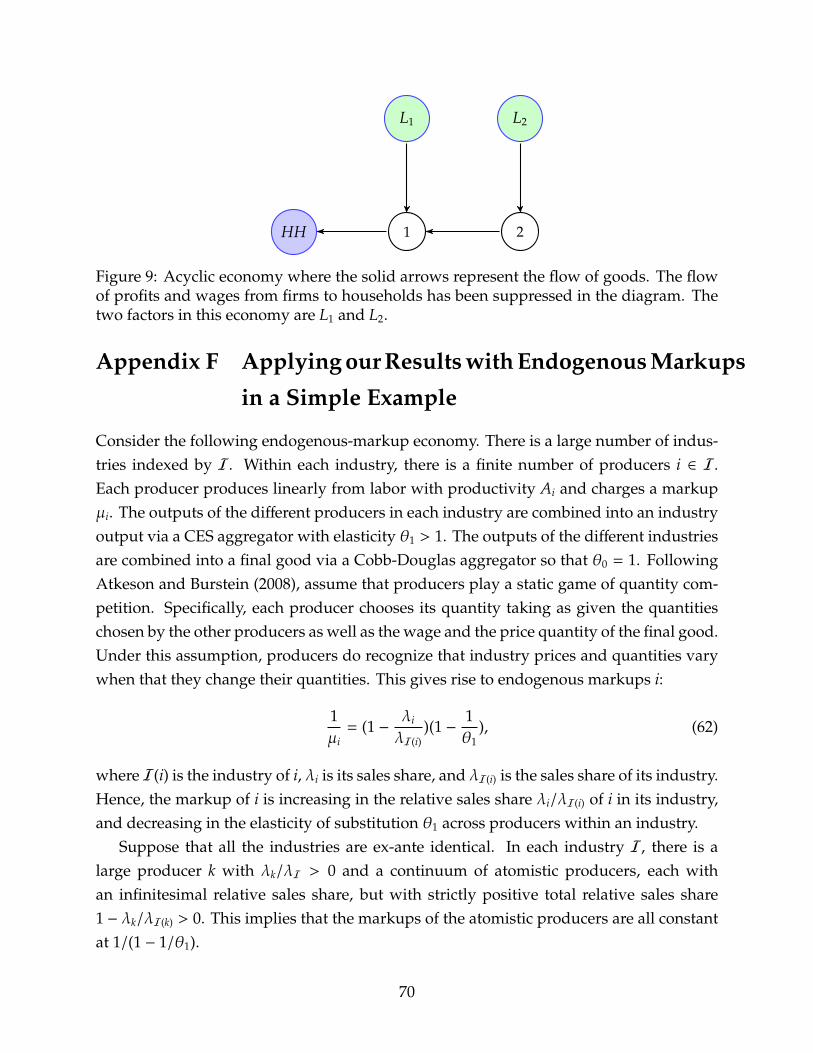
HH 1 2

L2L1

Figure 9: Acyclic economy where the solid arrows represent the flow of goods. The flowof profits and wages from firms to households has been suppressed in the diagram. Thetwo factors in this economy are L1 and L2.

Appendix F Applying our Results with Endogenous Markups

in a Simple Example

Consider the following endogenous-markup economy. There is a large number of indus-tries indexed by I. Within each industry, there is a finite number of producers i ∈ I.Each producer produces linearly from labor with productivity Ai and charges a markupµi. The outputs of the different producers in each industry are combined into an industryoutput via a CES aggregator with elasticity θ1 > 1. The outputs of the different industriesare combined into a final good via a Cobb-Douglas aggregator so that θ0 = 1. FollowingAtkeson and Burstein (2008), assume that producers play a static game of quantity com-petition. Specifically, each producer chooses its quantity taking as given the quantitieschosen by the other producers as well as the wage and the price quantity of the final good.Under this assumption, producers do recognize that industry prices and quantities varywhen that they change their quantities. This gives rise to endogenous markups i:

1µi

= (1 −λi

λI(i))(1 −

1θ1

), (62)

where I(i) is the industry of i, λi is its sales share, and λI(i) is the sales share of its industry.Hence, the markup of i is increasing in the relative sales share λi/λI(i) of i in its industry,and decreasing in the elasticity of substitution θ1 across producers within an industry.

Suppose that all the industries are ex-ante identical. In each industry I, there is alarge producer k with λk/λI > 0 and a continuum of atomistic producers, each withan infinitesimal relative sales share, but with strictly positive total relative sales share1 − λk/λI(k) > 0. This implies that the markups of the atomistic producers are all constantat 1/(1 − 1/θ1).

70

Now consider a shock the productivity Ak of a single large producer k in a singleindustry I(k). The markup of producer i does not change if it is not in the industry of theshocked producer. The markup of an atomistic producer in the industry of the shockedproducer does not change. And we can solve jointly for the change d logµk in the markupof producer k and for the change d logλk in its sales share:

d logµk =λk/λI(k)

1 − λk/λI(k)d logλk, d logλk = (θ1 − 1)(1−λk/λI(k))(d log Ak −d logµk), (63)

where the first equation can be obtained by differentiating the markup equation (62),and where the second equation can be obtained by applying the propagation equationsin Propositions 2 and 3 applied to producer k’s sales share rather than to factor shares.This in turn implies that the markup µk of producer k increases endogenously with itsproductivity Ak according to

d logµk

d log Ak=

λkλI(k)

(θ1 − 1)

1 + λkλI(k)

(θ1 − 1)> 0. (64)

There is therefore imperfect pass-through of productivity shocks to prices. We thenuse the chain rule equation (16) with Z = log Ak, in conjunction with the expressionsfor d log Λ/d log Ak and for d log Λ/d logµk given by Propositions 2 and 3. We find thattaking into account the endogenous change of the markups responsible for imperfect pass-through, the change d log Y resulting from an increase d log Ak > 0 in the productivity ofproducer k is

d log Y =d log Yd log Ak

d log Ak +d log Yd logµk

d logµk

d log Akd log Ak

= λk

1 +1 − λk

λI(k)

1 + λkλI(k)

(θ1 − 1)

λiλI(k)

(θ1 − 1)

1 + λkλI(k)

d log Ak.

If instead markups were exogenously fixed, we would have

d log Y =d log Yd log Ak

d log Ak = λk

1 +

λkλI(k)

(θ1 − 1)

1 + λkλI(k)

d log Ak,

which is strictly higher. We therefore see that imperfect pass-through via endogenousmarkups mitigates the impact of the shock.

71

Appendix G Standard-Form for Nested CES Economies

Throughout this section, variables with over-lines are normalizing constants equal to thevalues in steady-state. Since we are interested in log changes, the normalizing constantsare irrelevant.3

Nested CES Economies in Standard Form

A CES economy in standard form is defined by a tuple (ω, θ, µ, F) and a set of normalizingconstants (y, x). The (N + F + 1) × (N + F + 1) matrix ω is a matrix of input-outputparameters where the first row and column correspond to the reproducible final good,the next N rows and columns correspond to reproducible goods and the last F rows andcolumns correspond to non-reproducible factors. The (N + 1) × 1 vector θ is a vectorof microeconomic elasticities of substitution. Finally, the N × 1 vector µ is a vector ofmarkups/wedges for the N non-final reproducible goods.4

The F factors are modeled as non-reproducible goods and the production function ofthese goods are endowments

y f

y f= 1.

The other N + 1 other goods are reproducible, and the production of a reproducible goodk can be written as

yk

yk= Ak

∑l

ωkl

(xkl

xkl

) θk−1θk

θkθk−1

,

where xlk are intermediate inputs from l used by k. Each producer charges a markup overits marginal cost µk. Producer 0 represents final-demand and its production function thefinal-demand aggregator so that

Y

Y=

y0

y0, (65)

where Y is output and y0 is the final good.Through a relabelling, this structure can represent any CES economy with an arbitrary

pattern of nests, markups/wedges and elasticities. Intuitively, by relabelling each CESaggregator to be a new producer, we can have as many nests as desired.

3We use normalized quantities since it simplifies calibration, and clarifies the fact that CES aggregatorsare not unit-less.

4For convenience we use number indices starting at 0 instead of 1 to describe the elements of ω and θ,but number indices starting at 1 to describe the elements of µ. We impose the restriction that ωi j ∈ [0, 1],∑

j ωi j = 1 for all 0 ≤ i ≤ N, ω f j = 0 for all N < f ≤ N + F, ω0 f = 0 for all N < f ≤ N + F, and ωi0 = 0 for all0 ≤ i ≤ N.

72

Consider some initial allocation with markups/wedges µ and productivity shiftersnormalized, without loss of generality, at A = 1. The normalizing constants (y, x) arechosen to correspond to this initial allocation. Let b and Ω be the corresponding vectorof consumption shares and cost-based input-output matrix. Then we must have ω0i = bi

and ω(i+1)( j+1) = Ωi j. From there, all the other cost-based and revenue-based input-outputobjects can be computed exactly as in Section 2.2.

Appendix H Robustness and Extensions

In this section, we discuss some of the extensions mentioned in the body of the paper.Specifically, we address in more detail how are results extend to situations with arbi-trary non-CES production functions, elastic factors, capital accumulation/dynamics, andnonlinearities. Proofs for the results are at the end of this section.

H.1 Beyond CES

The input-output covariance operator defined in Section 4 is a key concept capturing thesubstitution patterns in economies where all production and utility functions are nested-CES functions. In this section, we generalize this input-output covariance operator insuch a way that allows us to work with arbitrary production functions.

For a producer j with cost function C j, we define the Allen-Uzawa elasticity of substi-tution between inputs x and y as

θ j(x, y) =C jd2C j/(dpxdpy)

(dC j/dpx)(dC j/dpy)=ε j(x, y)

Ω jy,

where ε j(x, y) is the elasticity of the demand by producer j for input x with respect to theprice py of input y, and Ω jy is the expenditure share in cost of input y.

Note the following properties. Because of the symmetry of partial derivatives, wehave θ j(x, y) = θ j(y, x). Because of the homogeneity of degree one of the cost function inthe prices of inputs, we have the homogeneity identity

∑1≤y≤N+1+F Ω jyθ j(x, y) = 0.

We define the input-output substitution operator for producer j as

Φ j(Ψ(k),Ψ( f )) = −∑

1≤x,y≤N+1+F

Ω jx[δxy + Ω jy(θ j(x, y) − 1)]ΨxkΨy f , (66)

=12

EΩ( j)

((θ j(x, y) − 1)(Ψk(x) − Ψk(y))(Ψ f (x) −Ψ f (y))

), (67)

73

where δxy is the Kronecker symbol, Ψk(x) = Ψxk and Ψ f (x) = Ψx f , and the expectation onthe second line is over x and y. The second line can be obtained from the first using thesymmetry of Allen-Uzawa elasticities of substitution and the homogeneity identity.

In the CES case with elasticity θ j, all the cross Allen-Uzawa elasticities are identicalwith θ j(x, y) = θ j if x , y, and the own Allen-Uzawa elasticities are given by θ j(x, x) =

−θ j(1 − Ω jx)/Ω jx. It is easy to verify that we then recover the input-output covarianceoperator:

Φ j(Ψ(k),Ψ( f ) = (θk − 1)CovΩ( j)(Ψ(k),Ψ( f )).

Even outside the CES case, the input-output substitution operator shares many prop-erties with the input-output covariance operator. For example, it is immediate to verify,that: Φ j(Ψ(k),Ψ( f )) is bilinear and symmetric in Ψ(k) and Ψ( f ); Φ j(Ψ(k),Ψ( f )) = 0 wheneverΨ(k) or Ψ( f ) is a constant.

Luckily, it turns out that all of the results stated in Sections 4 and 5 can be generalizedto non-CES economies simply by replacing terms of the form (θ j − 1)CovΩ( j)(Ψ(k),Ψ( f )) byΦ j(Ψ(k),Ψ( f )).

Intuitively, Φ j(Ψ(k),Ψ( f )) captures the way in which j redirects demand expendituretowards f in response to proportional unit decline in the price of k. To see this, we make useof the following observation: the elasticity of the expenditure share of producer j on inputx with respect to the price of input y is given by δxy+Ω jy(θ j(x, y)−1). Equation (66) requiresconsidering, for each pair of inputs x and y, how much the proportional reduction Ψyk inthe price of y induced by a unit proportional reduction in the price of k causes producerj to increase its expenditure share on x (as measured by −Ω jx[δxy + Ω jy(θ j(x, y) − 1)]Ψyk)and how much x is exposed to f (as measured by Ψx f ).

Equation (67) says that this amounts to considering, for each pair of inputs x andy, whether or not increased exposure to k as measured by Ψk(x) − Ψk(y), corresponds toincreased exposure to i as measured by Ψi(x)−Ψi(y), and whether x and y are complementsor substitutes as measured by (θ j(x, y) − 1). If x and y are substitutes, and Ψk(x) − Ψk(y)and Ψ f (x) −Ψ f (y) are both positive, then substitution across x and y by k, in response toa shock to a decrease in the price of k, increases demand for f .

H.2 Elastic Factor Supplies

In this section, we fully flesh out one such extension by showing to generalize our analysisto allow for endogenous factor supplies.

To model elastic factor supplies, let G f (w f Y,Y) be the aggregate supply of factor f ,where w f Y is the price of the factor in the GDP deflator numeraire (w f is the price of

74

the factor in the nominal GDP numeraire) and Y is real aggregate income. Let ζ f =

∂ log G f/∂ log(w f Y) be the elasticity of the supply of factor f to its real wage, and γ f =

−∂ log G f/∂ log Y be its income elasticity. We then have the following characterization:

d log Yd log Ak

= %

λk −

∑f

11 + ζ f

Λ fd log Λ f

d log Ak

, (68)

andd log Yd logµk

= %

−λk −

∑f

11 + ζ f

Λ fd log Λ f

d logµk

, (69)

where % = 1/(∑

f Λ f1+γ f

1+ζ f).

With inelastic factors, a decline in factor income shares, ceteris paribus, increases outputsince it represents a reduction in the misallocation of resources and an increase in aggregateTFP. With elastic factor supply, the output effect is dampened by the presence of 1/(1+ζ f ) <1. This is due to the fact that a reduction in factor income shares, while increasing aggregateTFP, reduces factor payments and factor supplies, which in turn reduces output. Hence,when factors are elastic, increases in allocative efficiency from assigning more resourcesto more monopolistic producers are counteracted by reductions in factor supplies due tothe associated suppression of factor demand.5

We can provide an explicit characterization of d log Λ f and d log Y in terms of microe-conomic elasticities of substitution in a nested-CES structure similar to the one in Section4. Changes in factor shares and output solve the following system of equations:

d log Λ f = −∑

k

λkΨk f

Λ fd logµk+

∑j

(θ j−1)λ j

µ jCovΩ( j)(

∑k

Ψ(k)d log Ak−

∑k

Ψ(k)d logµk,Ψ( f )

Λ f)

−

∑j

(θ j − 1)λ j

µ jCovΩ( j)(

∑g

Ψ(g)1

1 + ζgd log Λg +

∑g

Ψ(g)γg − ζg

1 + ζgd log Y,

Ψ( f )

Λ f),

d log Y = ρ

∑k

λkd log Ak −

∑k

λkd logµk −

∑f

Λ f1

1 + ζ fd log Λ f

.5In the limit where factor supplies become infinitely elastic, the influence of the allocative efficiency

effects disappear from output, since more factors can always be marshaled on the margin at the samereal price. To see this, consider the case with a single factor called labor, and factor supply functionGL(wY,Y) = Y−ν(wY)ν, which can be derived from a standard labor-leisure choice model. In this case,ζL = γL = ν, and so equation (68) implies that d log Y/d log Ak = λk − 1/(1 + ν) d log ΛL/d log Ak. Whenlabor supply becomes infinitely elastic ν → ∞, this simplifies to d log Y/d log Ak = λk, so that changes inallocative efficiency have no effect on output, even though they affect TFP.

75

Equations (68) and (69) can also be applied to frictionless economies with endogenousfactor supplies. They show that even without any frictions, Hulten’s theorem cannot beused to predict how output will respond to microeconomic TFP shocks, due to endogenousresponses of factors. These results therefore also extend Hulten’s theorem to efficienteconomies with endogenous factor supplies.

H.3 Capital Accumulation, Adjustment Costs, and Capacity Utilization

In mapping this set-up to the data, there are two ways to interpret this model: either wecould interpret final demand as a per-period part of a larger dynamic problem, or wecould interpret final demand as an intertemporal consumption function where goods arealso indexed by time a la Arrow-Debreu. When we interpret the model intratemporally,the output function encompasses demand for consumption goods and for investmentgoods. When we interpret the model intertemporally, the process of capital accumulationis captured via intertemporal production functions that transform goods in one periodinto goods in other periods. This modeling choice would also be well-suited to handletechnological frictions to the reallocation of factors such as adjustment costs and variablecapacity utilization. Our formulas would apply to these economies without change, but ofcourse, in such a world, input-output definitions would now be expressed in net-presentvalue terms.

H.4 Nonlinear Impact of Shocks and Duality with Industry Structure

Another limitation of our results is that we neglect nonlinearities. As discussed by Baqaeeand Farhi (2017a), models with production networks can respond very nonlinearly to pro-ductivity shocks. We plan to extend these results to inefficient economies in full generality,but as a first step, we stipulate some conditions under which we can directly leveragethese results to inefficient economies. In particular, we show that the amplification ofnegative shocks due to complementarities emphasized in Baqaee and Farhi (2017a) canalso work to amplify the negative effects of misallocation.

Consider the quantitative parametric model in Section 7. Let δk(i), µk(i), and Ak(i)denote firm i in industry k’s share of industry sales, markup, and productivity. Defineindustry k’s average markup and productivity to be

µk =

∑i

δk(i)µk(i)

−1

76

and

Ak/Ak =µk/µk(∑

i δk(i)(µk(i)/µk(i)

Ak(i)/Ak(i)

)1−ξk) 1

1−ξk

,

where overline variables denote steady-state values.To the original firm-level economy, we associate a dual industry-level economy, for

which the input output-matrix is aggregated at the industry level. Define the output levelof the dual economy by Y and the revenue-based Domar weight of industry k by λk. Thedual industry-level economy has initial industry-level markups equal to

µk =

∑i

δk(i)µk(i)

−1

.

The next proposition shows that productivity and markup shocks in the original firm-leveleconomy can be translated into productivity and markup shocks in the dual industry-leveleconomy.

Proposition 6 (Exact Duality). The discrete (nonlinear) output response ∆ log Y to shocks toproductivities and markups of the original economy is equal to the output response ∆ log Y to thedual shocks to productivity and markups of the dual economy.

Corollary 3 (Efficient Duality). Consider an economy where µk = 1 for every k, and consider atransformation µk(i)(tk) which changes markups but maintains µk = 1. Then

d log Yd log tk

=d log Yd log tk

= λkd log Ak

d log tk(70)

andd2 log Yd log t2

k

=d2 log Yd log t2

k

= λkd log λk

d log Ak

(d log Ak

d log tk

)2

+ λkd2 log Ak

d log t2k

, (71)

where d log λk/d log Ak is given by the formulas in Baqaee and Farhi (2017a).

If firms within an industry are substitutes, then increases in the dispersion of markups,which keep the harmonic average of markups equal to one, are isomorphic to negativeproductivity shocks in a model which is efficient at the industry level. Hence, shockswhich increase markup dispersion in an industry can have outsized nonlinear effects onoutput, if those industries are macro-complementary with other industries in the sensedefined by Baqaee and Farhi (2017a) so that d log λk/d log Ak < 0.

77

This helps flesh out the insight in Jones (2011) that complementarities can interact withdistortions to generate large reductions in output, and that these can be quantitativelyimportant enough to explain the large differences in cross-country incomes. Given the ex-amples in Baqaee and Farhi (2017a), it should be clear how misallocation in a key industrylike energy production can significantly reduce output through macro-complementarities.Investigating these nonlinear forces more systematically is an interesting exercise that weleave for future work.

Proof of Proposition 6. To streamline the exposition, we focus on a single industry, and weuse different but more straightforward notation. Consider an industry where: all firms iuse the same upstream input bundle with cost C; firms transform this input into a firm-specific variety of output using constant return to returns to scale technology; each firm ihas productivity ai and charges a markup µi; the varieties are combined into a compositegood by a competitive downstream industry according to a CES production function withelasticity σ on firm i. Without loss of generality, and only for convenience, we normalizeall prices in steady-state to be equal to C, which means that we normalize the levels ofproductivities in steady state (and only in steady state) to be equal to the markups.

We denote the quantity of composite good produced as

Q =[∑

b1σ

i qσ−1σ

i

] σσ−1

. (72)

Firm i charges a price

pi =µi

aiC. (73)

The resulting demand for firm i’s variety is

qi = (pi

P)−σbiQ, (74)

where the price index is given by

P =[∑

bip1−σi

] 11−σ. (75)

Total profits are given by

Π =∑

i

(pi − C)(pi

P)−σbiQ. (76)

78

We solve out the price index and profits explicitly and get

P =

∑i

bi

(µi

ai

)1−σ

11−σ

C, (77)

Π =∑

i

(µi

ai−

1ai

)

µiai[∑

j b j

(µ j

a j

)1−σ] 11−σ

−σ

biCQ. (78)

For completeness we can also solve for the sales of each firm as a fraction of the sales ofthe industry

λi =piqi

PQ=

bi

(µiai

)1−σ

∑j b j

(µ j

a j

)1−σ . (79)

We want to understand how to aggregate this industry into homogenous industrywith productivity A and markup µ. These variables must satisfy

P =µ

AC, (80)

Π =(µA−

1A

)CQ. (81)

This implies that A and µ are the solutions of the following system of equations

µ

A=

∑i

bi

(µi

ai

)1−σ

11−σ

, (82)

(µA−

1A

)=

∑i

(µi

ai−

1ai

)

µiai[∑

j b j

(µ j

a j

)1−σ] 11−σ

−σ

bi. (83)

The solution is

A =1

[∑i bi

(µiai

)1−σ] 11−σ

−∑

i

(1 − 1

µi

) µiai∑ j b j

( µ ja j

)1−σ 1

1−σ

−σ

µiai

bi

, (84)

79

µ =

[∑i bi

(µiai

)1−σ] 11−σ

[∑i bi

(µiai

)1−σ] 11−σ

−∑

i

(1 − 1

µi

) µiai∑ j b j

( µ ja j

)1−σ 1

1−σ

−σ

µiai

bi

. (85)

We can also rewrite this in a useful way as

A =1[∑

i bi

(µiai

)1−σ] 11−σ

1∑i

1µi

(µiai

)1−σbi∑

j b j

( µ ja j

)1−σ

=1[∑

i bi

(µiai

)1−σ] 11−σ

1∑i

1µiλi, (86)

µ =1∑

i1µi

(µiai

)1−σbi∑

j b j

( µ ja j

)1−σ

=1∑

i1µiλi. (87)

The theorem follows by applying this analysis to an industry k, with δk(i) = λi andbi = δk(i).

Appendix I Aggregation of Cost-Based Domar Weights

In this Appendix we show that recovering cost-based Domar weights from aggregateddata is, in principle, not possible. The vertical economy in Figure 1a also shows the failureof the aggregation property implied by Hulten’s theorem. The easiest way to see this is toconsider aggregating the input-output table for the economy in Figure 1a. For simplicity,suppose that markups are the same everywhere so that µi = µ for all i. Since there is nopossibility of reallocation in this economy, and since markups are uniform, this is our bestchance of deriving an aggregation result, but even in this simplest example, such a resultdoes not exist. Suppose that we aggregate the whole economy S = 1, . . . ,N. Then, inaggregate, the economy consists of a single industry that uses labor and inputs from itselfto produce. In this case, the input-output matrix is a scalar, and equal to the intermediateinput share of the economy

ΩSS =1 − 1

µN−1

1 − 1µN

, (88)

80

and the aggregate markup for the economy is given by µ. Therefore, λS constructed usingaggregate data is

λS = 1′(I − µΩ)−1 =µN−1

−1µ

1 − 1µ

. (89)

However, we know from the example that

d log Yd log A

=∑i∈S

λi = N , λS =µN−1

−1µ

1 − 1µ

, (90)

except in the limiting case without distortions µ→ 1. Therefore, even in this simplest case,with homogenous markups and no reallocation, aggregated input-output data cannot beused to compute the impact of an aggregated shock.

Appendix J Extra Examples

Example J.1. We build a simple example to underscore the importance of properly ac-counting for the multiplicity of factors to assess the macroeconomic impact of microeco-nomic shocks in inefficient economies. The example is depicted in Figure 10.

HH

1

23

L

K

Figure 10: An economy with two factors of production L and K. The subgraph fromL to the household contains a cycle, and hence can be subject to misallocation. On theother hand, there is only a unique path connecting K to the household, so there is nomisallocation.

We have

Γ = −(θ0 − 1)

Covb(Ψ(L),Ψ(L)) Covb(Ψ(K),Ψ(L))Covb(Ψ(L),Ψ(K)) Covb(Ψ(K),Ψ(K))

, (91)

and

δ(i) = (θ0 − 1)

Covb(Ψ(i),Ψ(L))Covb(Ψ(i),Ψ(K))

.Substituting in the values and solving the system of equations (11), using Proposition 2,

81

and noting that λi = λi for all i, we find that

d log Yd log Ai

= λi + λi(θ0 − 1)

1 −µ−1

iλ1

λ1+λ2µ−1

1 + λ2λ1+λ2

µ−12

, (i = 1, 2)

butd log Yd log Ai

= λi, (i = 3).

A lesson is that changes in allocative efficiency are only present for shocks to producers 1and 2 which share a factor of production, but not for producer 3 which has its own factorof production. Moreover, the changes in allocative efficiency for shocks to producers 1and 2 only depends on the markups of these two producers and not on the markup ofproducer 3.

Example J.2. We consider a simple example with two elasticities of substitution, whichdemonstrates the principle that changes in misallocation are driven by how each nodeswitches its demand across its supply chain in response to a shock. To this end, we applyProposition 2 to the economy depicted in Figure 11.

HH

1

3 4

L

2

Figure 11: An economy with two elasticities of substitution.

d log Yd log A3

=λ3 −1

ΛL

((θ0 − 1)

[b1(ω13µ

−11 (ω13µ

−13 + ω14µ

−14 )) − ω13b1ΛL

]+(θ1 − 1)µ−1

1 λ1

[ω13µ

−13 − ω13

(ω13µ

−13 + ω14µ

−14

)]).

82

The term multiplying (θ0 − 1) captures how the household will shift their demand across1 and 2 in response to the productivity shock, and the relative degrees of misallocation in1 and 2’s supply chains. The term multiplying (θ1 − 1) takes into account how 1 will shiftits demand across 3 and 4 and the relative amount of misallocation of labor between 3 and4. Not surprisingly, if instead we shock industry 1, then only the household’s elasticity ofsubstitution matters, since industry 1 will not shift its demand across its inputs in responseto the shock to industry 2:

d log Yd log A1

=b1 −1

ΛL(θ0 − 1)

[b1µ

−11 (ω13µ

−13 + ω14µ

−14 ) − b1ΛL

].

This illustrates the general principle in Proposition 2 that an elasticity of substitution θ j

matters only if j is somewhere downstream from k.

Example J.3. We build a simple example to illustrate the macroeconomic impact of mi-croeconomic markup/wedge shocks and their difference with microeconomic productivityshocks.

We consider a Cobb-Douglas economy, which helps to isolate the importance of the newterm in Proposition 3. For a Cobb-Douglas economy, the only source factor reallocationcomes from the fact that the producer which increases its markup/wedge releases somelabor. Let θ j = 1 for every j, which is the Cobb-Douglas special case. Now, applyingProposition 3, we get

d log Yd logµk

= −λk + λkΨkL

ΛL= −λk

(1 −

λk

λk

ΨkL

ΛL

).

As before, ΨkL/ΛL is a measure of how distorted the supply chain of k is relative to theeconomy as a whole. If ΨkL/ΛL < 1, then this means that for each dollar k earns, asmaller share reaches workers than it would if that dollar was spent by the household. Inother words, producer k’s supply chain has inefficiently too few workers. On the otherhand, λk/λk is a measure of how distorted the demand of chain of k is. If λk/λk < 1, thisimplies that k is facing double-marginalization. When the product of the downstreamand upstream terms is less than one, this means that producer k is inefficiently starved ofdemand and workers. Hence, an increase in the markup/wedge of k reduces the allocativeefficiency of the economy. On the other hand, when the product of these two terms isgreater than one, the path connecting the household to labor via producer k is too large.Therefore, an increase in the markup/wedge of k reallocates resources to the rest of theeconomy where they are more needed and increases allocative efficiency.

83

With multiple factors, we get

d log Yd logµk

= −λk + λk

∑f

Λ fΨk f

Λ f= −λk

1 −λk

λk

∑f

Λ fΨk f

Λ f

.This generalizes the intuitions discussed earlier for markup/wedge shocks in the Cobb-Douglas economy with a single factor to the case of multiple factors. In particular, theamount of factor f released by sector k as a fraction of total factor f per unit of shock isλkΨk f/Λ f and the impact of that release on output per unit of shock is Λ f . We also seeagain the roles of the index of downstream distortions λk/λk and of the generalized indexof upstream distortions

∑f Λ f Ψk f/Λ f .

Example J.4. We consider an example showing how, in general, the correlation betweenproductivity and wedges matters. Consider the horizontal economy example discussed inSection 5.1, but instead of assuming log-normality, consider the binomial case where Ai ∈

0,A with probability 1/2 and ∆ logµi ∈ 0,∆ logµ with probability 1/2. An immediateapplication of formula (19) shows that L ≈ (1/8)θ0(∆ logµ)2 if Ai and µi are independent,but that L ≈ 0 if Ai and µi are perfectly correlated.

Appendix K Volatility of Aggregate TFP

In this section, we use the quantitative structural model of Section 7.3 to assess thevolatility of aggregate output arising from firm-level and industry-level productivity andmarkup shocks.6 For this section, we do not assume that each Compustat firms’ share ofindustry sales in Compustat is the same as its share of total industry sales in the BEA data.Instead, we assign to each firm its actual sales, and assume that any leftover sales aresold by a residual producer whose markup is equal to the average industry-level markupand who experiences no shocks (this effectively means we assume that the residual (non-Compustat) producer in each industry is really a representative of a mass of infinitesimalfirms and experiences no shocks due to the law of large numbers).

We use our ex-post structural results on the elasticities of aggregate output to theseshocks

log Y ≈ log Y +∑

i

d log Yd log Ai

d log Ai +∑

i

d log Yd logµi

d logµi,

6When we consider firm-level shocks, we assess only the contribution of shocks to Compustat firms, i.e.we account for the macro-volatility arising from firm-level shocks when only Compustat firms are beingshocked, and not non-Compustat firms. We focus on this exercise because we do not have the data requiredto compute the contribution of shocks to all firms.

84

to approximate the implied volatility of output in response to microeconomic shocks.Assuming productivity shocks and markup shocks are independent and identically dis-tributed, get

Var(log Y) ≈∑

i

(d log Yd log Ai

)2

Var(d log Ai) +∑

i

(d log Yd logµi

)2

Var(d logµi),

= ‖Dlog A log Y‖2Var(d log A) + ‖Dlogµ log Y‖2Var(d logµ).

Hence, the Euclidean norm ‖Dlog A log Y‖ of the Jacobian of log Y with respect to log Agives the degree to which microeconomic productivity shocks are not “diversified” awayin the aggregate. Similarly, ‖Dlogµ log Y‖ measures the diversification factor relative tomarkup shocks.7

Table 3 displays the diversification factor, for both markup shocks and productivityshocks at the firm level and at the industry level, for our benchmark model. We also com-pute the results for a Cobb-Douglas distorted economy where all elasticities are unitary, aswell as for a perfectly competitive model without wedges. Across the board, the distortedmodel is more volatile than the competitive model, however the extent of this dependsgreatly on the type of shock and the level of aggregation. We discuss these different casesin turn.

First, consider the case of productivity shocks: as mentioned previously, the benchmarkmodel is more volatile than the perfectly competitive model for both sets of shocks.However, the more interesting comparison is with respect to the distorted Cobb-Douglaseconomy. As explained in Section 4, the allocation of factors is invariant to productivityshocks in the Cobb-Douglas model. Hence, the Cobb-Douglas model lacks the reallocationchannel, and hence can tell us in which direction the reallocation force is pushing. Inthe case of industry-level shocks, the benchmark model is slightly less volatile than theCobb-Douglas model, whereas in the case of firm-level shocks, the benchmark model issignificantly more volatile.

A partial intuition here relates to the elasticities of substitution: whereas industriesare complements, firms within an industry are strong substitutes. Recall that looselyspeaking, changes in allocative efficiency scale with the elasticity of substitution minusone. Firm-level shocks cause a considerable amount of changes in allocative efficiencywhereas industry-level shocks cause much milder changes. At both levels of aggregation,

7Although Baqaee and Farhi (2017a) suggest that log-linear approximations can be unreliable for model-ing the mean, skewness, or kurtosis of output in the presence of microeconomic shocks, their results indicatethe log-linear approximations of variance are less fragile (although still imperfect). In the final section ofthis paper, we discuss how our results can be extended to understanding the nonlinear impact of shocks.

85

Benchmark Competitive Cobb-Douglas Constant X

Firm Productivity Shocks (UC) 0.0491 0.0376 0.0396 0.0396Firm Markup Shocks (UC) 0.0296 0.0000 0.0077 0.0000Industry Productivity Shocks (UC) 0.3162 0.3118 0.3259 0.3259Industry Markup Shocks (UC) 0.0084 0.0000 0.0391 0.0000

Firm Productivity Shocks (AP) 0.0524 0.0376 0.0415 0.0415Firm Markup Shocks (AP) 0.0368 0.0000 0.0085 0.0000Industry Productivity Shocks (AP) 0.3188 0.3118 0.3375 0.3375Industry Markup Shocks (AP) 0.0127 0.0000 0.0500 0.0000

Firm Productivity Shocks (PF) 0.0598 0.0376 0.0398 0.0398Firm Markup Shocks (PF) 0.0321 0.0000 0.0112 0.0000Industry Productivity Shocks (PF) 0.3299 0.3418 0.3618 0.3618Industry Markup Shocks (PF) 0.0216 0.0000 0.0760 0.0000

Table 3: Diversification factor for different productivity and markup shocks at firm andindustry level for different specifications of the model. A diversification factor of 1 meansthat the variance of microeconomic shocks moves aggregate variance one-for-one. Adiversification factor of 0 means that microeconomic shocks are completely diversifiedaway at the aggregate level. The final column is the allocation that holds the allocationmatrix X constant in response to shocks.

86

these changes in allocative efficiency amplify some shocks and mitigate some otherscompared to the Cobb-Douglas model with no change in allocative efficiency.8 On thewhole, at the firm level, the changes in allocative efficiency are so large that they dwarf thepure technology effects picked up by the Cobb-Douglas model and amplify the volatilityof these shocks. By contrast, at the industry level, changes in allocative efficiency are moremoderate and turn out to slightly mitigate the volatility of these shocks.

These intuitions are confirmed in the first two columns of Figure 12, where we plot theoutput elasticity with respect to productivity shocks to specific firms or industries relativeto their revenue-based Domar weight. This represents a comparison of our benchmarkmodel to a competitive model where Hulten’s theorem holds. We find considerabledispersion in the response of the model relative to both, but much more so at the firmlevel than at the industry level. We could plot the same graph but with the cost-basedDomar weight as a reference point in order to represent the comparison of our benchmarkmodel to the Cobb-Douglas model, and the results would be visually similar.

Next, consider the effects of markup shocks. In this case, the distorted Cobb-Douglaseconomy is not necessarily a very natural benchmark since even with Cobb-Douglas,shocks to markups will reallocate factors across producers. Nonetheless, it is still instruc-tive to compare the benchmark model to the Cobb-Douglas one to find that a similarlesson applies as with productivity shocks. The volatility of firm-level shocks is amplifiedrelative to Cobb-Douglas while the volatility of industry-level shocks is attenuated rela-tive to Cobb-Douglas. This follows from the fact that industries are more complementarythan firms, and hence, in line with the intuition from the horizontal economy, the effectof the shock are monotonically increasing in the degree of substitutability. The last twocolumns of Figure 12 plot the output elasticity with respect to markup shocks to specificfirms or industries relative to their revenue-based Domar weight.

Online References

Ackerberg, D. A., K. Caves, and G. Frazer (2015). Identification properties of recentproduction function estimators. Econometrica 83(6), 2411–2451.

Atkeson, A. and A. Burstein (2008). Pricing-to-market, trade costs, and internationalrelative prices. American Economic Review 98(5), 1998–2031.

8There is another difference: reallocation occurs towards the firm receiving a positive shock; but reallo-cation occurs away from the industry receiving a positive shock.

87

−5.00 0.00 5.000

100

num

ber

(a)

−5.00 0.00 5.000

100

200

num

ber

(b)

0.80 1.00 1.200

20

*

num

ber

(c)

−0.10 −0.05 0.00 0.050

10

*

num

ber

(d)

Figure 12: The left column contains histograms of d log Y/d log A and the rightd log Y/d logµ relative to λ for firm-level and industry-level shocks respectively. Thetop row are shocks to firms and the bottom row are shocks to industries. The bunchingat the extremes, winsorizing at 4 standard deviations, marked with a star arise solely fordisplaying purposes. In all cases, the degree of dispersion around the response impliedby the competitive model (the size of the producer) is substantial.

88

Baqaee, D. R. and E. Farhi (2017). The macroeconomic impact of microeconomic shocks:Beyond Hulten’s Theorem.

Claus, J. and J. Thomas (2001). Equity premia as low as three percent? evidence fromanalysts’ earnings forecasts for domestic and international stock markets. The Journal ofFinance 56(5), 1629–1666.

De Loecker, J., J. Eeckhout, and G. Unger (2019). The rise of market power and themacroeconomic implications. Technical report, National Bureau of Economic Research.

Gutierrez, G. and T. Philippon (2016). Investment-less growth: An empirical investigation.Technical report, National Bureau of Economic Research.

Hall, R. E. (1988). The relation between price and marginal cost in us industry. Journal ofpolitical Economy 96(5), 921–947.

Jones, C. I. (2011). Intermediate goods and weak links in the theory of economic develop-ment. American Economic Journal: Macroeconomics, 1–28.

Levinsohn, J. and A. Petrin (2003). Estimating production functions using inputs to controlfor unobservables. The review of economic studies 70(2), 317–341.

Olley, G. S. and A. Pakes (1996). The dynamics of productivity in the telecommunicationsequipment industry. Econometrica: Journal of the Econometric Society, 1263–1297.

89