Misallocation, Selection and Productivity: A QuantitativeAnalysis with Panel Data from China†

Tasso AdamopoulosYork University

Loren BrandtUniversity of Toronto

Jessica LeightWilliams College

Diego RestucciaUniversity of Toronto and NBER

January 2017

Abstract

We use household-level panel data from China and a quantitative framework to document the ex-tent and consequences of factor misallocation in agriculture. We find that there are substantialfrictions in both the land and capital markets linked to land institutions in rural China that dispro-portionately constrain the more productive farmers. These frictions reduce aggregate agriculturalproductivity in China by affecting two key margins: (1) the allocation of resources across farmers(misallocation) and (2) the allocation of workers across sectors, in particular the type of farm-ers who operate in agriculture (selection). We show that selection can substantially amplify thestatic misallocation effect of distortionary policies by affecting occupational choices that worsen thedistribution of productive units in agriculture.

JEL classification: O11, O14, O4.Keywords: agriculture, misallocation, selection, productivity, China.

†We are grateful to Chaoran Chen for providing excellent research assistance. We also thank for useful commentsCarlos Urrutia, Daniel Xu, and seminar participants at Toronto, McGill, Ottawa, REDg Barcelona, NBER Chinaworkshop, IMF conference on inequality, Cornell, Michigan, UBC, Xiamen U., ASU, Tsinghua-USCD China confer-ence, HKUST macroeconomics conference, Western conference on misallocation, Tsinghua workshop on macroeco-nomics, EEA Geneva, Banco de Mexico, Montreal, Ohio State, and Universitat de Barcelona. Restuccia gratefullyacknowledges the support from the Canada Research Chairs program. Brandt thanks the support from the No-randa Chair for International Trade and Economics. Adamopoulos, Brandt, and Restuccia gratefully acknowledgethe support from the Social Sciences and Humanities Research Council of Canada. Contact: Tasso Adamopou-los, aadamo@yorku.ca; Loren Brandt, brandt@chass.utoronto.ca; Jessica Leight, jessica.leight@williams.edu; DiegoRestuccia, diego.restuccia@utoronto.ca

1

1 Introduction

A central theme in the study of economic growth and development is the large productivity differ-

ences in the agricultural sector across countries. Since labor in poor countries is primarily allocated

to agriculture, understanding these differences is essential in accounting for aggregate income dif-

ferences between rich and poor countries.1 Productivity gaps in agriculture between developing and

developed countries are also consistent with increasing evidence that resource misallocation across

households that are heterogeneous in skill is more prevalent in developing countries.2 Institutions

and policies giving rise to misallocation are highly pervasive in agriculture in poor countries and

can account for a large portion of the productivity differences across countries.3 These institutions

often diminish the efficiency of land and other complementary markets in directing resources to

their most productive uses.

We use micro farm-level panel data from China and a quantitative framework to document the

extent and consequences of factor misallocation in agriculture. We find that there are substantial

frictions in both the land and capital markets in rural China that disproportionately affect the more

productive farmers. We argue that these distortions reduce aggregate agricultural productivity

by affecting two key margins: (1) the allocation of resources across farmers (misallocation); and

(2) the allocation of workers across sectors, in particular, the type of farmers who operate in

agriculture (selection). The key insight of our paper is that selection can substantially amplify

the misallocation effect of distortionary policies by affecting occupational choices that worsen the

distribution of productive units in agriculture. Intuitively, institutions generating misallocation have

1See, for instance, Gollin et al. (2002), Restuccia et al. (2008).2See Restuccia and Rogerson (2008) and Hsieh and Klenow (2009). Restuccia and Rogerson (2013) review the

expanding literature on misallocation and productivity.3See, for instance, recent studies linking resource misallocation to land market institutions, such as land re-

forms in Adamopoulos and Restuccia (2015); the extent of marketed land across farm households in Restuccia andSantaeulalia-Llopis (2015); and the role of land titling in Chen (2016) and Gottlieb and Grobovsek (2015). de Janvryet al. (2014) study a land certification reform in Mexico delinking land rights from land use which allowed for a moreefficient allocation of individuals across space.

2

a particularly negative effect on more highly skilled farmers, who are then less likely to operate a

farm in agriculture, thereby reducing average agricultural productivity and widening even further

the productivity gap between the agricultural and non-agricultural sectors.

We focus on China for several reasons. First, China is a rapidly growing economy experiencing

substantial reallocation within and across sectors. Yet, productivity growth in agriculture has been

lackluster, especially in the cropping sector, the focus of this paper. Second, the operational size of

farm units in China is extremely small, only about 0.7 hectares on average, and has not increased

over time. This average size compares with 16 and 17 hectares in Belgium and the Netherlands,

countries with similar amounts of arable land per capita as China, and to 178 hectares in the United

States. Third, institutionally, there is a lack of well-defined property rights over land, which can lead

to both factor misallocation within agriculture and distortions of sectoral-occupational choices. And

fourth, we have a unique panel dataset of households with detailed input and output information

on all farm and non-farm activities over 1993-2002.4 The data allow us to construct precise real

measures of value added and productivity at the farm-level, and to observe the incomes of the same

households across sectors. In the context of a widespread shift into non-agricultural activity these

data offer a unique opportunity to examine the selection effect of distortionary policies.

Our goal is to measure the extent of misallocation across farmers implied by the land market institu-

tions in China, and to quantify its consequences for occupational choices, agricultural productivity,

and real GDP per capita, by combining our detailed panel-level data from China and a two-sector

model with selection and idiosyncratic distortions in agriculture.5

Our empirical approach combines micro-level data with economic theory. Basic producer theory

4The data are collected by the Research Center for the Rural Economy under the Ministry of Agriculture as partof a nation-wide survey.

5We do not study the effect of land market institutions on farm-level productivity. While insecurity over propertyrights may also affect the type of investments that households may make on their land (investments in irrigation anddrainage, long-term soil fertility, etc.) and other related investments, we focus on the role that insecure land rightsplay for the operation of land markets.

3

implies that in the absence of market frictions, marginal products of factors should be equalized

across farms, with more productive farmers operating larger farms and hiring more capital. However,

given land market institutions in China, we expect this basic principle to be violated, as more

productive farmers are unable to accumulate additional land. This will show up as a gap in marginal

products of land, with more productive farmers having a higher marginal product. Even if there

is no other friction in capital markets, the friction in the land market will induce a gap between

marginal products of capital as well since the more productive farmers will now utilize less capital.

To measure the deviations between marginal products and the overall extent of static inefficiency,

we use a diagnostic tool from modern macroeconomics, a heterogeneous firm-industry framework

with minimal structure. In this set-up, the land market institutions in China manifest themselves

as “wedges” in marginal products, with the property that these wedges are larger for farmers with

higher productivity. We find that the output (productivity) gains from reallocation are sizable.

Nationally, reallocating capital and land across existing farmers to their efficient use would in-

crease aggregate agricultural output and TFP by 84 percent. Reallocation within villages—a much

narrower geographical definition of reallocation—is a substantial contributor to these gains, rep-

resenting 60 percent of the overall gains. Distortions across farms with different productivity and

distortions among farms with the same productivity contribute equally to the overall reallocation

gains. Moreover, we do not find substantial changes in the extent of misallocation over time, con-

sistent with an absence of substantial changes in China’s land market institutions over this period.

We then embed the agricultural framework into a two-sector model of agricultural and nonagricul-

tural production in order to study the impact of misallocation in agriculture on the selection of

individuals across sectors. We use the equilibrium properties of the model to calibrate the parame-

ters to observed moments and targets from the micro data for China. In particular, the substantial

reallocation of households from agriculture to non-agriculture, and their cross-sector income corre-

lation, allow us in our framework to pin down the population correlation of abilities across sectors.

4

We then conduct a series of counterfactual experiments to assess the quantitative importance of mis-

allocation and its overall impact on aggregate agricultural productivity, accounting for distortions

in sectoral occupational choices. We emphasize three sets of counterfactuals.

First, we assess the effect of misallocation on aggregate productivity by eliminating all distortions.

This counterfactual generates a large 13.8-fold increase in agricultural labor productivity; a signifi-

cant increase in agricultural TFP of 4.3-fold; and a substantial reallocation of labor across sectors,

with the share of employment in agriculture falling from 46 percent to 5 percent. The total effect

on agricultural productivity is substantially larger than the static effect of eliminating misallocation

across existing farmers. The difference is due to the substantial amplification effect that distortions

have on the selection of farmers in the model, which produces an additional increase in agricul-

tural TFP of 2.6-fold. That is, selection more than doubles the impact of reduced misallocation on

agricultural productivity.

Second, to isolate the contribution of correlated distortions (i.e., the property of distortions that they

increase with farm productivity), we eliminate only these distortions by setting their correlation with

agricultural ability to zero. This results in an increase of agricultural productivity of more than 11-

fold, which is about 92 percent of the increase in productivity from eliminating all distortions. This

implies that although correlated and uncorrelated distortions to agricultural activity contribute

equally to misallocation in China, it is the systematic component of distortions affecting more

heavily the more productive farmers, which is responsible for most of the amplification effect on

productivity through distorted occupational choices and selection.

And third, we compare the productivity gains from eliminating “static” misallocation in the previous

counterfactual with an equivalent increase in economy-wide productivity. We find that there is

no additional increase in agricultural productivity in this case and the share of employment in

agriculture falls to only 29 percent compared to 5 percent when eliminating distortions. Distortions

in the agricultural sector generate much larger selection effects than comparable changes in economy-

5

wide TFP because distortions have a direct impact on occupational choices instead of just the general

equilibrium effects generated via common shifts in production parameters.

Our paper contributes to the broad literature on misallocation and productivity by addressing two

essential issues emphasized recently in Restuccia and Rogerson (2016). First, we link misallocation

to specific policies/institutions, in our context, land market institutions in China.6 Second, we

study the broader impact of misallocation, in particular, the effect of distortionary policies on

misallocation and the selection of skills across sectors, which substantially amplifies the productivity

losses from factor misallocation. In this context, our paper relates to the role of selection highlighted

in Lagakos and Waugh (2013). A key difference in our work is that we empirically document the role

of distortions in the agricultural sector as the key driver of low agricultural productivity and show

that these distortions generate much larger effects on selection than equivalent changes in economy-

wide TFP. Moreover, the panel dimension of the data allows us to identify a key parameter in these

selection models that captures the correlation of abilities across sectors with important implications

for aggregate outcomes. We underline that in our calibration economy-wide changes in TFP have

no amplification effects on agricultural productivity; hence, our selection results are distinct from

Lagakos and Waugh (2013) in that they are solely driven by the impact of idiosyncratic distortions

on occupational choices.

The paper proceeds as follows. In the next section, we describe the specifics of the land market in-

stitutions in China which are intertwined with additional mobility restrictions across space through

the “hukou” registration system. Section 3 presents the basic framework for identifying distortions

and measuring the gains from reallocation. In Section 4, we describe the panel data from China and

the variables we use in our analysis. We construct in Section 5 measures of household-farm produc-

tivity and present the main results on misallocation in agriculture in China. Section 6 embeds the

6Our paper also relates to earlier studies of the Chinese economy emphasizing the role of agriculture (Lin, 1992;Zhu, 2012); the importance of misallocation across provinces and between the state and non-state sectors (Brandtet al., 2013); and growth in economic transition in Song et al. (2011). Tombe and Zhu (2015) and Ngai et al. (2016)analyze the important impact of migration restrictions in the “hukou” system for reallocation and welfare in China.

6

framework of agriculture into a heterogeneous-ability two-sector model with non-agriculture. We

calibrate the model to aggregate, sectoral, and micro moments from the Chinese data in Section 7.

Section 8 reports the main results from our quantitative experiments. We conclude in Section 9.

2 Land Market Institutions in China

The Household Responsibility System (HRS), established in rural China in the early 1980s, disman-

tled the system of collective management set up under Mao and extended use rights over farmland

to rural households. These reforms triggered a spurt in productivity growth in agriculture in the

early 1980s that subsequently dissipated. This level effect is often attributed to the improved effort

incentives for households as they became residual claimants in farming (McMillan et al., 1989; Lin,

1992). Ownership of agricultural land however remained vested with the collective, and in partic-

ular the village or small group, a unit below the village. Use rights to land were administratively

allocated among rural households by village officials on a highly egalitarian basis that reflected

household size. In principle, all individuals with “registration” (hukou), in the village were entitled

to land.

The law governing the HRS provided secure use rights over cultivated land for 15 years (in the late

1990s use rights were extended to 30 years), however village officials often reallocated land among

households before the 15-year period expired. Benjamin and Brandt (2002) document that in over

two-thirds of all villages reallocations occurred at least once, and on average more than twice. Their

survey data show that reallocations undertaken between 1983-1995 typically involved three-quarters

of all households in the village, and most of village land. A primary motivation of the reallocations

was to accommodate demographic changes within a village. In addition, village officials reallocated

land from households with family members working off the farm to households solely engaged in

agriculture (Brandt et al., 2002; Kung and Liu, 1997).

7

In principle, households had the right to rent or transfer their use rights to other households

(zhuanbao), however in practice these rights were abridged in a variety of ways, resulting in thin

land rental markets. Brandt et al. (2002) document that in 1995, while 71.6 percent of villages

reported no restrictions on land rental activity, households rented out less than 3 percent of their

land, with most rentals occurring among family members or close relatives, hence not necessarily

directing the land to the best uses. The limited scope for farm rental activity is frequently associated

with perceived “use it or lose it” rules: Households that did not use their land and either rented

it to others or let it lie fallow risked losing the land during the next reallocation. As a result,

households may have been deterred from renting out land because of fear that it may be viewed by

village officials as a signal that the household did not need the land (see, for example, Yang, 1997).

Finally, we note that lack of ownership of the land also meant that households could not use it as

collateral for purposes of borrowing.

The difficulty in consolidating land either through land purchases or land rentals is one of the reasons

that operational sizes of farms have been typically very low in China and have not changed much

over time. According to the World Census of Agriculture of the Food and Agricultural Organization

in 1997 average farm size in China was 0.7 hectares. Contrast this to the United States where in the

same year average farm size was 187 hectares or to Belgium and the Netherlands—two developed

countries with similar arable land per person as China—where average farm size is around 16-17

hectares. Moreover, in developed countries, farm size is growing over time.7

The administrative egalitarian allocation of land combined with the limited scope for land rentals

implied that more able farmers or those that valued land more highly were not able to increase

operational farm size. To the extent that village officials either do not observe farmer ability

(unobserved heterogeneity) or do not make land allocation decisions based on ability (egalitarian

7Small operational farm scales are not unique to China, as average farm sizes among the poorest countries inthe world are below 1 hectare and also reflect low productivity in agriculture, see for instance Adamopoulos andRestuccia (2014).

8

concerns), reallocations were unhelpful in improving operational scale and productivity (Benjamin

and Brandt, 2002). These frictions in the land market could generate allocative inefficiency or

misallocation by distorting the allocation of land across farmers. Also, the inability to use land as

collateral for borrowing purposes could result in the misallocation of other inputs such as capital.

Further, the distortions faced in agriculture may affect the occupational choices of individuals

between working in agriculture or other sectors of the economy, thus affecting the type of farmer

that remains in agriculture. The interaction of allocative inefficiency with distortions in occupational

choices can affect agricultural productivity and overall development.

In the next sections we describe our basic framework, the panel data we use for China, and the two-

sector model with selection, which allows us to quantify the broader consequences of misallocation

for occupational choices, aggregate agricultural productivity, and real GDP per capita.

3 Basic Framework for Measuring Misallocation

We describe the industry framework we use to assess the extent of misallocation in agriculture

in China. We derive the efficient allocations that maximize agricultural output given a set of

inputs, and then contrast these to the actual allocations. The ratio of efficient to actual output

characterizes the potential gains from an efficient reallocation. We rationalize the actual allocations

as an equilibrium of this framework with input and output wedges, which enables us to use the

equilibrium equations to identify farmer-specific input and output distortions from the data. We

then use these wedges to construct a summary measure of distortions faced by each farmer in China.

9

3.1 Description

We consider a rural economy that produces a single good and is endowed with amounts of farm land

L and capital K, and a finite number M of farm operators indexed by i. Following Adamopoulos

and Restuccia (2014), the production unit in the rural economy is a family farm. A farm is a

technology that requires the inputs of a farm operator (household), as well as the land and capital

under the farmer’s control. Farm operators are heterogeneous in their farming ability si.8

As in Lucas Jr (1978), the production technology available to farmer i with productivity si exhibits

decreasing returns to scale in variable inputs and is given by the Cobb-Douglas function,

yi = (Aasi)1−γ [`αi k1−αi

]γ, (1)

where y, `, and k denote real farm output, land, and capital. The parameter Aa is a common

productivity term, γ < 1 is the span-of-control parameter which governs the extent of returns to

scale at the farm-level, and α captures the relative importance of land in production.

3.2 Efficient Allocation

Our starting point is the static efficient allocation of factors of production obtained from the solution

to a simple planner’s problem that takes the distribution of productivities as given. We use this

efficient allocation and the associated maximum aggregate agricultural output as a benchmark to

contrast with the actual (distorted) allocations and the agricultural output in the Chinese economy.

The planner chooses how to allocate land and capital across farmers in the rural economy to

8For ease of exposition and tractability our framework abstracts from differences across farmers in the intensivemargin of labor input. We deal with this by adjusting outputs and inputs in the data, generating a residual measureof farm TFP that is unaffected by this abstraction. We note however that since labor days may also be misallocated,our estimates of misallocation from this framework may be conservative.

10

maximize aggregate agricultural output subject to aggregate resource constraints. Specifically, the

problem of the planner is:

max{ki,`i}Mi=1

M∑i=1

yi,

subject to

yi = (Aasi)1−γ (`αi k1−αi

)γ, i = 1, 2, ...M ;

and the resource constraints,M∑i=1

`i = L;M∑i=1

ki = K. (2)

Using the first-order conditions to this problem along with the rural economy-wide resource con-

straints in equation (2), the efficient allocation involves allocating total land and capital across

farmers according to relative productivity,

`ei =si∑Mj=1 sj

L, (3)

kei =si∑Mj=1 sj

K, (4)

where the superscript e denotes the efficient allocation. Equations (3) and (4) indicate that in the

efficient allocation, more productive farmers are allocated more land ` and capital k.

Using the definition of aggregate agricultural output Y =∑M

i=1 yi along with individual technologies

and input allocations as derived above, we obtain a rural economy-wide production function,

Y e = AeM1−γ [LαK1−α]γ ,where Y e is aggregate agricultural output under the efficient allocation, Ae is agricultural TFP

Ae =(AaS

)1−γ, where S =

(∑Mi=1 si

)/M is average farm productivity.

11

3.3 Equilibrium and Identification of Distortions

We estimate farm-specific distortions as implicit input and output wedges or taxes. These taxes

are abstract representations that serve to rationalize as an equilibrium outcome the actual observed

allocations in the Chinese economy. While this representation is not required for assessing the

aggregate consequences of misallocation—since we can directly compare efficient allocations and

output with the actual data—it will be useful in the estimation of the two-sector economy in

Section 6 and the subsequent counterfactual exercises. Denote by τ `i and τ ki the land and capital

input taxes, and by τ yi the output tax faced by farm i. Tax revenues are equally distributed lump-

sum across all households. With two factors of production we can separately identify farm-specific

distortions to either land and capital or output and one of the two inputs. We solve the farmer

problem subject to all the farm-specific taxes and then show the identification issue that arises.

Given distortions, the profit maximization problem facing farm i is,

max`i,ki

{πi = (1− τ yi ) yi −

(1 + τ ki

)rki −

(1 + τ `i

)q`i},

where q and r are the rental prices of land and capital. In equilibrium, the land and capital markets

for the rural economy must clear as in equation (2).

We use this framework to identify the farm-specific distortions from the observed land and capital

allocations across farmers. In our abstraction these distortions are induced by “taxes” but in

practice they arise from China’s land market institutions. In particular, the first-order conditions

with respect to land and capital for farm i imply:

MRPLiαγ

=yi`i

=q(1 + τ `i

)αγ (1− τ yi )

∝(1 + τ `i

)(1− τ yi )

, (5)

12

MRPKi

(1− α)γ=yiki

=r(1 + τ ki

)(1− α)γ (1− τ yi )

∝(1 + τ ki

)(1− τ yi )

, (6)

where MRPL and MRPK are the marginal revenue products of land and capital, respectively.

Given that we normalize the price of agricultural goods to one, MRPL and MRPK are also

the marginal products of the respective factors. Equations (5) and (6) show that in the presence

of farm-specific distortions, average products and marginal products of land and capital are not

equalized across farms, but rather vary in proportion to the idiosyncratic distortion faced by each

factor relative to the output distortion.

Equations (5)-(6) imply two things. First, only two of the three taxes can be separately identified.

Either taxes on the two inputs{τ ki , τ

`i

}Mi=1

or the output tax and one of the two input taxes, i.e.,{τ `i , τ

yi

}Mi=1

or{τ ki , τ

yi

}Mi=1

. Second, farm-specific distortions can be identified up to a scalar from

the average product of each factor.9

We construct the following summary measure of distortions faced by farm i,

TFPRi =yi

`αi k1−αi

= TFPR

(1 + τ `i

)α (1 + τ ki

)1−α(1− τ yi )

, (7)

where TFPR ≡(

qαγ

)α (r

(1−α)γ

)1−αis the common component across all farms. We note that

TFPR corresponds to the concept of “revenue productivity” in Hsieh and Klenow (2009), and use

this notation to make the analogy clear. Equation (7) indicates that TFPRi is proportional to a

geometric average of the farm-specific land and capital distortions relative to the output distortion.

We emphasize that TFPR is different from “physical productivity” or TFP, which in our model is,

TFPi ≡ (Aasi)1−γ =

yi[`αi k

1−αi

]γ , (8)

9The scalar for the land input common to all farms is qαγ , while the scalar for the capital input is r

(1−α)γ .

13

for farm i.10 In a world without distortions farms with higher physical productivity TFPi command

more land `i, and capital ki, and marginal products of each factor equalize across farms. However,

with idiosyncratic distortions this need not be the case as indicated by equations (5) and (6).

Using the fact that total output is Y =∑M

i=1 yi, we can derive the rural economy-wide production

function,

Y = TFP ·M1−γ [LαK1−α]γ , (9)

where (L,K) are total land and capital, and TFP is rural economy-wide TFP,

TFP =

Aa∑M

i=1 si

(TFPRTFPRi

) γ1−γ

M

1−γ

, (10)

with average revenue productivity TFPR given by

TFPR =TFPR[∑M

i=1yiY

(1−τyi )(1+τ`i )

]α [∑Mi=1

yiY

(1−τyi )(1+τki )

]1−α . (11)

Equation (10) makes clear that with no dispersion in TFPRi across farm households, the equilib-

rium allocations and aggregate output and TFP coincide with the corresponding efficient statistics.

Farm-level behavior in the presence of distortions aggregates up to a rural economy-wide produc-

tion function with aggregate land L, capital K, number of farmers M , and aggregate (distorted)

productivity TFP . Under the described identification of distortions from the data, allocations and

aggregate distorted output Y in the model coincide with actual observations in the data for China.

We measure aggregate agricultural output reallocation gains by comparing efficient output to ac-

tual output in the Chinese economy. Since aggregate factors K, L, and M are held fixed in this

comparison, the output gains represent TFP gains, i.e., Y e/Y = Ae/TFP .

10In Hsieh and Klenow (2009)’s terminology farm TFP is TFPQ.

14

4 Data

We use household survey data collected by the Research Center for the Rural Economy under

the Ministry of Agriculture of China.11 This is a nationally representative survey that covers all

provinces. The survey has been carried out annually since 1986 with the exception of 1992 and 1994

when funding was an issue. An equal number of rich, medium and poor counties were selected in

each province, and within each county a similar rule was applied in the selection of villages. Within

villages, households were drawn in order to be representative. Important changes in survey design

in 1993 expanded the information collected on agriculture, and enabled more accurate estimates of

farm revenues and expenditures.

We have data for ten provinces that span all the major regions of China, and use the data for

the period between 1993 and 2002. The data are in the form of an unbalanced panel. In each

year, we have information on approximately 8000 households drawn from 110 villages. For 104

villages, we have information for all 9 years. The average number of household observations per

village-year is 80, or a quarter to a third of all households in a village. We have data for all 9 years

for approximately 6000 households. Attrition from the sample is not a concern and is examined in

detail in Benjamin et al. (2005). Much of the attrition is related to exit of entire villages from the

survey. Household exit and entry into the sample is not systematically correlated with key variables

of interest. During the period of our study, migration of entire households was severely restricted.

The survey provides disaggregated information on household income and labor supply by activity.

For agriculture, we have data on total household land holdings, sown area and output by crop,

and major farm inputs including labor, fertilizer, and farm machinery. Regarding non-agricultural

activities, for family businesses we have information on revenues, expenditures, and net incomes

from each type of household non-family business. We also know household wage earnings.

11For a detailed description and analysis of the data see Benjamin et al. (2005).

15

The richness of the data on crops, inputs and prices, allows us to construct precise real measures

of output and productivity at the farm-level.

Value added agricultural output We utilize the detailed information on farm output by crop

in physical terms to construct estimates of “real” gross farm output. Output of each crop is valued

at a common set of prices, which are constructed as sample-wide averages (unit values) over 1993-

2002 for each crop. Unit values are computed using information on market sales, and are exclusive

of any “quota” sales at planned (below market) prices. In these calculations, a household’s own

consumption is implicitly valued at market prices. Intermediate inputs such as fertilizers and

pesticides are treated in an analogous way. We subtract expenditures on intermediate inputs from

gross output to obtain our estimate of net income or value added for the cropping sector. In what

follows, we use this measure of real value added at the farm-level when we refer to farm output.

Land, capital, and labor The measure of land that we use in our analysis is cultivated land by

the household, which corresponds to the concept of operated rather than “owned” farm size. The

survey provides household-level information beginning in 1986 on the value at original purchase

prices of farm machinery and equipment, larger hand tools, and draft animals used in agriculture.

Assuming that accumulation began in 1978, the year the reforms of the agricultural system began,

we utilize the perpetual inventory method to calculate the value of farm machinery in constant

Renminbi (RMB). The survey does not capture household ownership of smaller farm tools and

implements, and so for just over a third of household-years, the estimated value of their capital

stock is zero. To deal with these cases, we impute for all farm households a value equal to the

amount of land operated by the household multiplied by ten percent of the median capital to land

ratio by village-year. Robustness tests show that our results are not crucially sensitive to the

adjustment factor we use. For the labor input, we have the total labor days supplied on agricultural

activities by all members of the household and by hired labor.

16

5 Measuring TFP and Misallocation in Agriculture

We use the micro data from China to measure farm-level TFP and document the input allocations

in relation to farm TFP and the hypothetical efficient allocations. We next estimate the implicit

farm-specific distortions implied by our simple framework of Section 3. This provides an important

input for our two-sector analysis with selection in Section 6. We then report the static efficiency

gains for the agricultural sector in China from eliminating farm-specific distortions, providing a

benchmark number relative to which we can compare the efficiency gains that would result from

eliminating distortions in our two-sector model with selection.

5.1 Measuring Farm Productivity

Our measure of productivity at the farm-level is “physical productivity” or TFP, which we construct

residually from the farm-level production function in Section 3 using equation (8) and data on

operated land, capital, labor, and value added as described in Section 4. In our framework household

labor supply to agriculture is assumed to be the same across all households, however in the data

households differ in the number of days worked on the farm. To make a consistent mapping of the

data to model variables, we remove the variation in labor input by normalizing output, land, and

capital by total labor days. To see that this normalization results in a residual measure of farm

TFP that is not affected by labor supply differences, consider the extended production function in

equation (1) that includes labor supply, ni, by the household:

yi = (Aasini)1−γ[ˆαi k

1−αi

]γ,

where the hat variables distinguish these from the per labor days variables in our baseline framework.

Dividing both sides of this equation by ni, and defining variables in per labor days (i.e., yi = yi/ni)

17

yields the production function in equation (1). Our residual measure of idiosyncratic farm TFP

computed from equation (8) is also unaffected by differences in labor supply when y, k, and ` are

measured in per labor days.

Computing farm TFP from equation (8) requires values for the parameters γ and α. The values we

use are γ = 0.54, reflecting an income share of labor of 0.46, and α = 2/3, implying a land income

share of 0.36 and hence a capital income share of 0.18. These values represent the best estimates of

these shares we know for China. Some discussion of these is in order. Data on income shares for the

U.S. would attribute a similar income share of labor (same γ) but a larger income share for capital,

roughly reversing the shares of capital and land. If the capital-to-land ratios across farmers were

constant in the data, this alternative calibration using U.S. shares would imply the same overall

reallocation gains, and only change the relative contribution of capital and land to these gains.

Because capital-to-land ratios are not constant across farmers in our data (the capital to land ratio

is larger in less productive farms), the reallocation gain results would be larger using a larger capital

share as implied by a calibration to US data. In this context, our choices of production elasticities

are conservative with respect to the reallocation gains we highlight below.

We find that the dispersion in farm TFP in our data is substantial, with the standard deviation

of log–farm TFP equal to 0.72. The 90/10 percentile ratio in farm TFP is 6-fold whereas the

75/25 percentile ratio is 2.4-fold. While this dispersion in farm-level TFP is substantial, it is lower

than the dispersion of farm TFP in Malawi reported in Restuccia and Santaeulalia-Llopis (2015)

and in plant-level TFP documented in Hsieh and Klenow (2009) for Indian, Chinese and U.S.

manufacturing. For instance, in China the 90/10 ratio of plant-level TFP is 12.7-fold whereas the

75/25 ratio is 3.8-fold.

18

5.2 Factor Allocations and Productivity

If land and capital were allocated across farms in a decentralized fashion through unhindered factor

markets, the resulting allocations would resemble the efficient allocations in Section 3.2, with rela-

tively more productive farmers employing more land and capital. In other words, the relationship

between input use and TFP would be strongly positive. In addition, we would expect marginal

(and average) products of factors to be unrelated with farm TFP since in an efficient world these

marginal products are equalized.

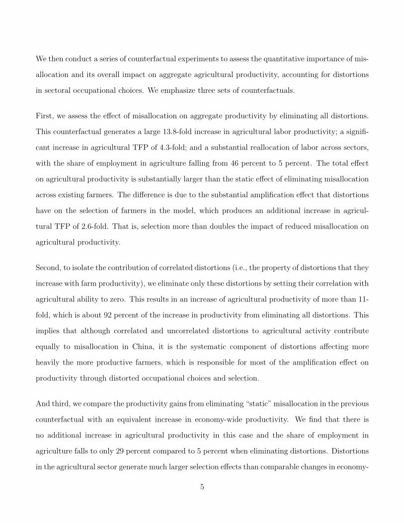
In fact, in the case of China we observe the exact opposite patterns. Figure 1 documents the

patterns of farm allocations in land and capital by farm-level TFP (in logs) for the year 2000. Land

use and capital use are not systematically positively correlated with farm productivity in China.12

In addition, the average productivity (output per unit of input) of land and capital inputs are

systematically positively correlated with farm TFP across farms in China. These patterns are not

consistent with an efficient allocation of resources across farmers in China (red dotted lines). They

are however consistent with the institutional setting in China we described in Section 2 including

the fairly uniform administrative allocation of land among members of the village. The lack of

ownership over the allocated plots (and hence inability to use land as collateral) can also partly

rationalize the misallocation of capital. Overall, the land market institutions in China prevent the

flow of resources to the most productive farmers.

5.3 Distortions and Productivity

The input allocations across farmers in China indicate that there is substantial misallocation. In the

context of the decentralized framework we presented in Section 3, this misallocation is manifested

12If anything capital use appears to be slightly negatively correlated with farm TFP. This slight negative correlationmay be due to other frictions in the capital market, some of which are discussed in Brandt et al. (2013).

19

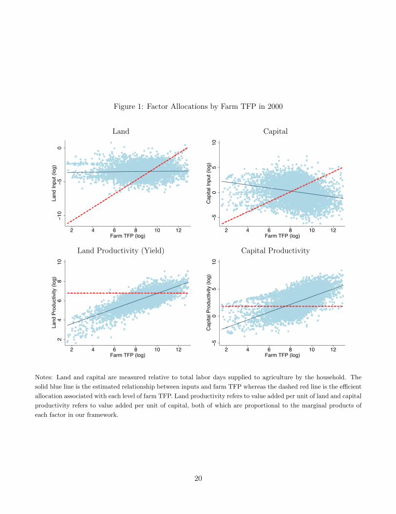
Figure 1: Factor Allocations by Farm TFP in 2000

Land Capital

−10

−50

Land

Inpu

t (lo

g)

2 4 6 8 10 12Farm TFP (log)

−50

510

Cap

ital I

nput

(log

)

2 4 6 8 10 12Farm TFP (log)

Land Productivity (Yield) Capital Productivity

24

68

10La

nd P

rodu

ctiv

ity (l

og)

2 4 6 8 10 12Farm TFP (log)

−50

510

Cap

ital P

rodu

ctiv

ity (l

og)

2 4 6 8 10 12Farm TFP (log)

Notes: Land and capital are measured relative to total labor days supplied to agriculture by the household. The

solid blue line is the estimated relationship between inputs and farm TFP whereas the dashed red line is the efficient

allocation associated with each level of farm TFP. Land productivity refers to value added per unit of land and capital

productivity refers to value added per unit of capital, both of which are proportional to the marginal products of

each factor in our framework.

20

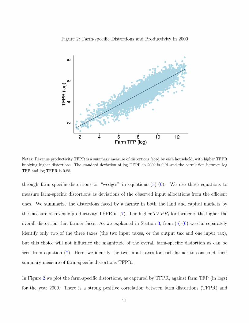
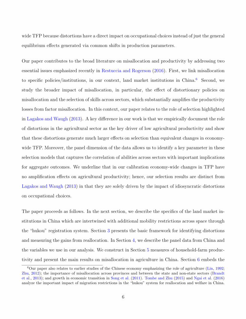
Figure 2: Farm-specific Distortions and Productivity in 2000

24

68

TFPR

(log

)

2 4 6 8 10 12Farm TFP (log)

Notes: Revenue productivity TFPR is a summary measure of distortions faced by each household, with higher TFPR

implying higher distortions. The standard deviation of log TFPR in 2000 is 0.91 and the correlation between log

TFP and log TFPR is 0.88.

through farm-specific distortions or “wedges” in equations (5)-(6). We use these equations to

measure farm-specific distortions as deviations of the observed input allocations from the efficient

ones. We summarize the distortions faced by a farmer in both the land and capital markets by

the measure of revenue productivity TFPR in (7). The higher TFPRi for farmer i, the higher the

overall distortion that farmer faces. As we explained in Section 3, from (5)-(6) we can separately

identify only two of the three taxes (the two input taxes, or the output tax and one input tax),

but this choice will not influence the magnitude of the overall farm-specific distortion as can be

seen from equation (7). Here, we identify the two input taxes for each farmer to construct their

summary measure of farm-specific distortions TFPR.

In Figure 2 we plot the farm-specific distortions, as captured by TFPR, against farm TFP (in logs)

for the year 2000. There is a strong positive correlation between farm distortions (TFPR) and

21

productivity (TFP), with the correlation equal to 0.88.13 The more productive farmers face higher

farm-specific distortions. This relationship reflects the nature of the land market institutions in

China. The administrative egalitarian allocation of land, along with the thin rental land markets,

provide little scope for farmers to adjust the operational size of the farm they are “endowed” with.

The farmers hurt the most from such an institutional setting are the more productive ones who

would have wanted to expand the most in unfettered markets, acquiring more land and capital. In

the context of our decentralized framework, this is reflected in higher farm-specific distortions on

the more productive farmers.

5.4 Static Efficiency Gains

In order to measure the efficiency gains associated with the misallocation of resources in agriculture

we conduct a counterfactual exercise. We ask how much larger would aggregate output (and as

a result TFP) be in agriculture if all farm-specific distortions were eliminated holding constant

aggregate resources? The efficiency gains from eliminating misallocation are given by the ratio of

the efficient to the (distorted) observed total output, Y e/Y .

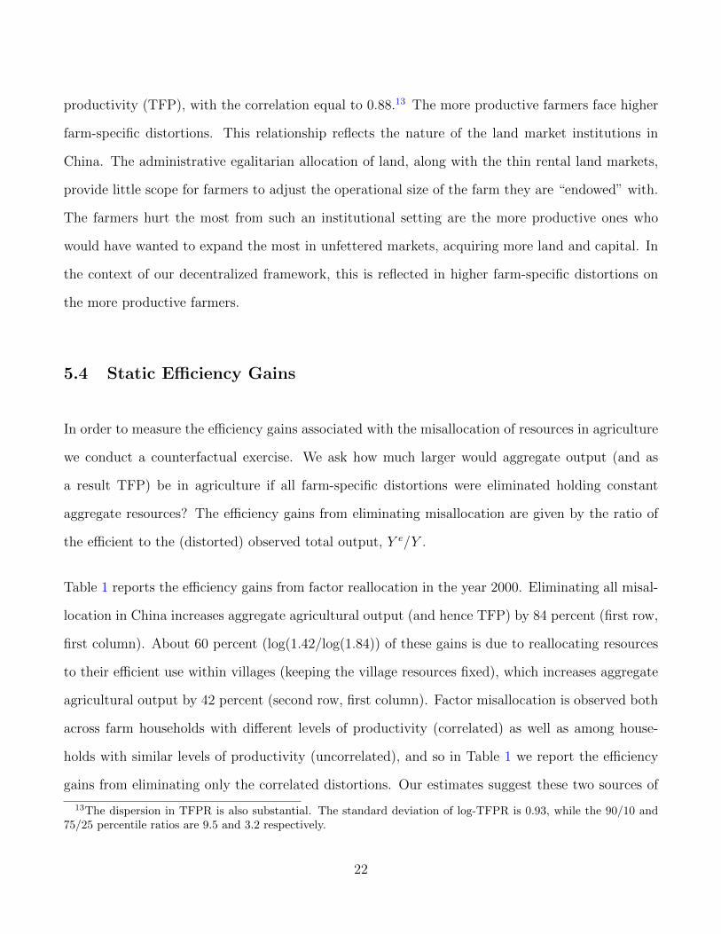
Table 1 reports the efficiency gains from factor reallocation in the year 2000. Eliminating all misal-

location in China increases aggregate agricultural output (and hence TFP) by 84 percent (first row,

first column). About 60 percent (log(1.42/log(1.84)) of these gains is due to reallocating resources

to their efficient use within villages (keeping the village resources fixed), which increases aggregate

agricultural output by 42 percent (second row, first column). Factor misallocation is observed both

across farm households with different levels of productivity (correlated) as well as among house-

holds with similar levels of productivity (uncorrelated), and so in Table 1 we report the efficiency

gains from eliminating only the correlated distortions. Our estimates suggest these two sources of

13The dispersion in TFPR is also substantial. The standard deviation of log-TFPR is 0.93, while the 90/10 and75/25 percentile ratios are 9.5 and 3.2 respectively.

22

misallocation contribute equally to the efficiency gains from reallocation (log(1.37)/log(1.84)=0.52).

Table 1: Efficiency Gains from Reallocation (year 2000)

Output (TFP) GainBaseline Across s Average

Misallocation Productivity

Eliminating misallocation:nationwide 1.84 1.37 1.67within village 1.42 1.16 1.33

Notes: The table reports the output gain from efficient reallocation as the ratio of efficient to actual aggregate agri-

cultural output. The column “Across s Misallocation” refers to the reallocation gains only eliminating misallocation

across farm households with different productivity and the column “Average Productivity” refers to the realloca-

tion gains when farm TFP is given by the fixed effect of farm TFP in the panel data to isolate the non-transitory

component of productivity.

Table 1 also reports the gains from efficient reallocation in 2000 using an average measure of farm

TFP rather than actual TFP in 2000. That is, we estimate the farm household fixed effect in

the panel data to isolate non-transitory components of productivity. Because TFP growth in the

cropping sector for the period we study in our data is zero, the fixed effect of productivity equals

average productivity for each household. The reallocation gain is 67 percent rather than the 84

percent in our baseline, implying that 84 percent of the reallocation gains are due to misallocation

of inputs across the non-transitory component of productivity.

While there are not explicit prohibitions of rentals in China, we noted in the description of the insti-

tutional setting in Section 2 that frequent reallocations of land within villages likely lead households

to fear loss of their use rights if they do not farm their land themselves. Indeed, rental markets are

very thin in China during our sample period, constituting less than 5 percent of cultivated land.

Moreover, there is no significant change in the amount of rented land over time. In addition, rentals

of land typically involve family members or close relatives and hence do not necessarily direct the

land to best uses. Nevertheless, we can assess the extent to which rented land alleviates misallo-

23

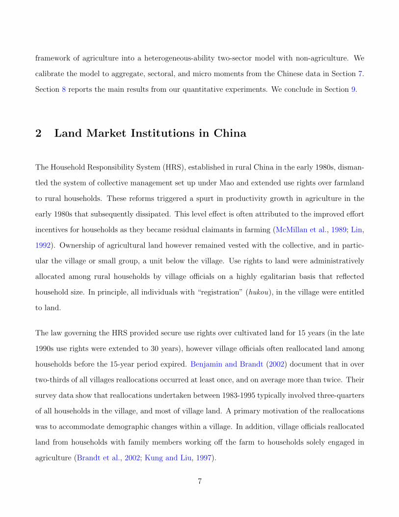
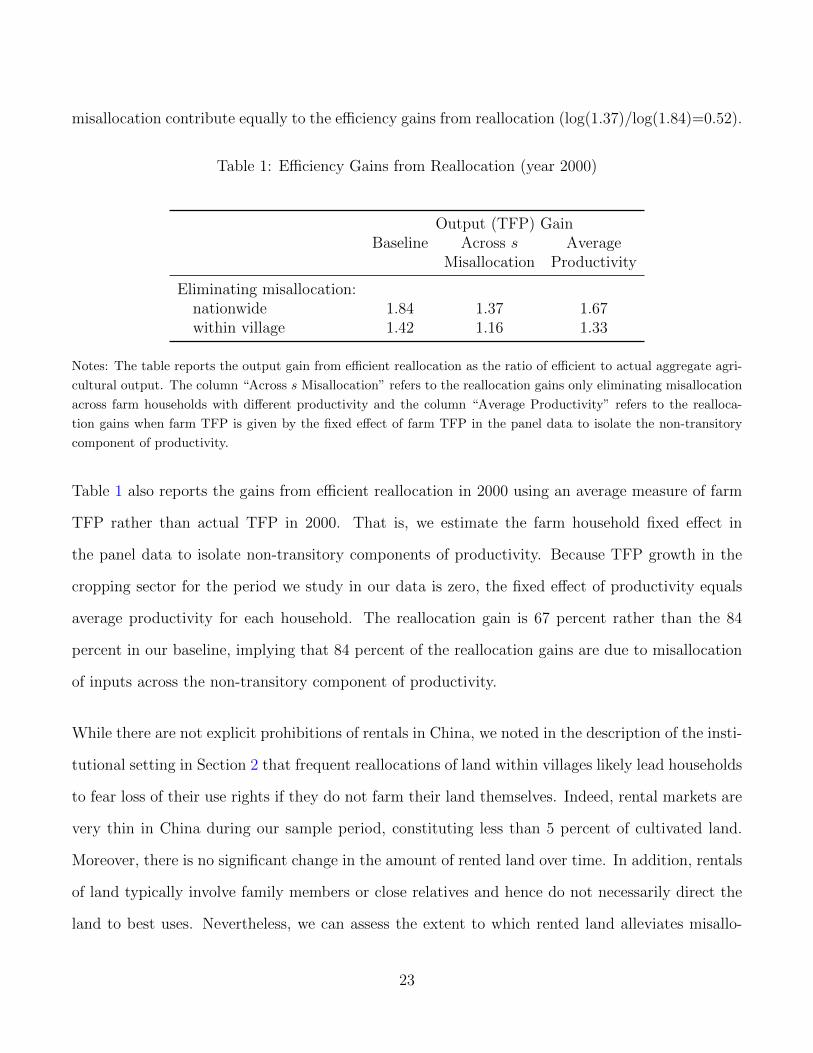
Figure 3: Evolution of Efficiency Gains of Reallocation over Time

1992 1993 1994 1995 1996 1997 1998 1999 2000 2001 2002 2003Year

1

1.2

1.4

1.6

1.8

2

2.2

2.4

2.6Ef

ficie

ncy

Gai

ns

NationwideWithin Village

Notes: Efficiency gains are reported as the ratio of efficient output to actual output (i.e., Y e/Y ) nationwide or as

the average across villages.

cation. Controlling for farm TFP, we find that the reallocation gains among farms with no rented

land are 20 percent larger than among farms with some rented land. This suggests that rentals

help reduce misallocation but their scale is too limited to prevent large productivity losses due to

misallocation.

Figure 3 reports the annual output gains of efficient reallocation, that is, the ratio of efficient to

actual output, for each year from 1993 to 2002. Importantly, there is no substantial change in the

magnitude of the misallocation in the rural sector, and thus the gains from reallocation over time

in China. If anything, misallocation seems to be slightly increasing. This finding contrasts with the

reduction in misallocation found for the manufacturing sector in China in Hsieh and Klenow (2009)

24

over a similar period. Within-village misallocation of capital and land across farmers is a substantial

source of reallocation gains, an increase in output (and hence TFP) of around 40 percent. When

capital and land are efficiently allocated across all farmers in China, the increase in output is nearly

80 percent in the 1990’s and almost 90 percent in 2002. These findings are consistent with the view

of costly farm-specific distortions that are tied to land market institutions in China that have not

changed much over the period we study.

6 Misallocation and Selection across Sectors

We now integrate our framework of agriculture into a standard two-sector general-equilibrium Roy

(1951) model of selection across sectors to assess: (1) how farm-specific distortions in agriculture

alter the occupational choice of individuals between agriculture and non-agriculture; and (2) how

selection affects measured misallocation in the agricultural sector and the productivity gains from

factor reallocation.

We augment our model of agriculture along the following dimensions. First, we extend the model

to a two-sector model by introducing a non-agricultural sector. Second, we consider preferences

for individuals over consumption goods for agriculture and non-agriculture, with a subsistence

constraint for the agricultural good. Third, individuals are endowed with a pair of productivities,

one for each of the two sectors. Fourth, individuals make an occupational choice of whether to

become farm operators in agriculture or workers in the non-agricultural sector. We show that a

key determinant of the occupational choice is the farm-specific distortion individuals face if they

become farm operators. For analytical tractability, we consider a continuum of individuals. The

fraction of individuals that choose agriculture, and thus the number and productivity distribution

of farms are endogenous. In what follows, we describe the economic environment in detail, defining

the equilibrium and describing some key properties of the model.

25

6.1 Environment

At each date there are two goods produced, agricultural (a) and non-agricultural (n). The non-

agricultural good is the numeraire and we denote the relative price of the agricultural good by pa.

The economy is populated by a measure 1 of individuals indexed by i.

Preferences Each individual i has preferences over the consumption of the two goods given by,

Ui = ω log (cai − a) + (1− ω) log(cni),

where ca and cn denote the consumption of the agricultural and non-agricultural good, a is a

minimum subsistence requirement for the agricultural good, and ω is the preference weight on

agricultural goods. The subsistence constraint implies that when income is low a disproportionate

amount will be allocated to the agricultural good. Individual i faces the following budget constraint,

pacai + cni = Ii + T,

where Ii is the individual’s income, and T the transfer to be specified below.

Working in the agricultural sector involves operating a farm and is subject to idiosyncratic dis-

tortions, captured by ϕi < 1, in order to fit the Chinese factor allocations by productivity in

agriculture as we specify below. Income from working in the non-agricultural sector is subject to a

tax η < 1, common to all individuals. η operates as a barrier to labor mobility from agriculture to

non-agriculture and is meant to capture the factors that restrict access to off-farm opportunities for

farmers. Quantitatively, this parameter allows us to fit the ratio of agricultural to non-agricultural

labor productivity.

26

Individual abilities and distortions Individuals are heterogeneous with respect to their abil-

ities in agriculture and non-agriculture, and the farm-specific distortions they face in agriculture.

In particular, each individual i is endowed with a pair of sector-specific abilities (sai, sni) and an

idiosyncratic farm distortion ϕi. The triplet (sai, ϕi, sni) is drawn from a known population joint

trivariate distribution of skills and distortions with density f (sai, ϕi, sni) and cdf F (sai, ϕi, sni). We

allow for the possibility that skills are correlated across sectors, and that agricultural skills (but

not non-agricultural skills) are correlated with farm-specific distortions. In particular, we assume a

trivariate log-normal distribution for (sai, ϕi, sni) with mean (µa, µϕ, µn) and variance,

Σ =

σ2a σaϕ σan

σaϕ σ2ϕ 0

σan 0 σ2n

.

We denote the correlation coefficient for abilities across sectors by ρan = σan/(σnσa), and the

correlation coefficient between agricultural ability and farm-specific distortions by ρϕa = σϕa/(σϕσa).

Individuals face two choices: (a) a consumption choice, the allocation of total income (including

transfers) between consumption of agricultural and non-agricultural goods; and (b) an occupational

choice, whether to work in the non-agricultural sector or the agricultural sector. We denote the

income an individual i would earn in agriculture as Iai and that in non-agriculture as Ini, and

the individual chooses the sector with the highest income. We denote by Hn and Ha, the sets of

(sai, ϕi, sni) values for which agents choose each sector Hn = {(sai, ϕi, sni) : Iai < Ini}, and Ha =

{(sai, ϕi, sni) : Iai ≥ Ini}.

Consumption allocation To determine the allocation of income between agricultural and non-

agricultural goods individuals maximize utility subject to their budget constraint, given their income

Ii + T , and the relative price of the agricultural good pa.The first order conditions to individual i’s

27

utility maximization problem imply the following consumption choices,

cai = a+ω

pa(Ii + T − paa) , cni = (1− ω) (Ii + T − paa) .

Production in non-agriculture The non-agricultural good is produced by a stand-in firm with

access to a constant returns to scale technology that requires only effective labor as an input,

Yn = AnZn,

where Yn is the total amount of non-agricultural output produced, An is non-agricultural produc-

tivity (TFP), and Zn is the total amount of labor input measured in efficiency units, i.e., accounting

for the ability of workers Zn =∫i∈Hn snidi. The total number of workers employed in non-agriculture

is,

Nn =

∫i∈Hn

di.

The representative firm in the non-agricultural sector chooses how many efficiency units of labor to

hire in order to maximize profits. The first order condition from the representative firm’s problem

in non-agriculture implies wn = An.

Production in agriculture As described previously, the production unit in the agricultural

sector is a farm. A farm is a technology that requires the inputs of a farm operator with ability sai

as well as land (which also defines the size of the farm) and capital under the farmer’s control. The

farm technology exhibits decreasing returns to scale and takes the form used previously,

yai = (Aasai)1−γ (`αi k1−αi

)γ, (12)

28

where ya is real farm output, ` is the land input, and k is the capital input. Aa is an agriculture-

specific TFP parameter, common across all farms.

An individual that chooses to operate a farm faces an overall farm-specific tax on output τi, which

summarizes the farm-specific taxes on output τ yi , and inputs(τ `i , τ

ki

)from Section 3,

(1− τi) ≡(1− τ yi )(

1 + τ `i)α (

1 + τ ki)1−α .

Note that in the data (1− τi) is constructed as a summary of the distortions faced by each farm,

as identified in Section 5. Tax revenues are redistributed equally to the N workers independently

of occupation, and equal to T per individual.

The profit maximization problem for farm i is given by,

max`i,ki{πi = pa (1− τi) yai − rki − q`i} , (13)

where (q, r) are the rental prices of land and capital. The first-order conditions to farm operator

i’s problem imply that farm size, demand for capital input, output supply, and profits depend not

only on productivity but also on the farm-specific distortions,

`i = Aa (γpa)1

1−γ

(1− αr

) γ(1−α)1−γ

(α

q

) 1−γ(1−α)1−γ

(1− τi)1

1−γ sai, (14)

ki = Aa (γpa)1

1−γ

(1− αr

) 1−αγ1−γ

(α

q

) αγ1−γ

(1− τi)1

1−γ sai, (15)

yai = Aa (γpa)γ

1−γ

(1− αr

) γ(1−α)1−γ

(α

q

) αγ1−γ

(1− τi)γ

1−γ sai, (16)

πi = Aa (1− γ) p1

1−γa γ

γ1−γ

(1− αr

) γ(1−α)1−γ

(α

q

) αγ1−γ

(1− τi)1

1−γ sai. (17)

29

The income of a farmer is the (after-tax) value of their output Iai = pa (1− τi) yai. As a result

farmer income includes not only the return to the farmer’s labor input π but also the land and

capital incomes. We can re-write an individual’s income from agriculture as,

Iai = waϕisai, (18)

where ϕi ≡ (1− τi)1

1−γ captures the overall farm-specific distortion faced by farmer i, and wa is the

component of the farmer’s income that is common to all farmers,

wa ≡ p1

1−γa Aaγ

γ1−γ

(1− αr

) γ(1−α)1−γ

(α

q

) αγ1−γ

. (19)

Note that wa summarizes the effects of relative prices as it is a function of the endogenous relative

price of agriculture pa, the rental price of land q, and the rental price of capital r.

Similarly, we can re-write land input demand, capital input demand, output supply and profits for

farmer i in terms of their agricultural ability and farm-specific distortions,

`i = ¯ϕisai; ki = kϕisai; yai = yaϕγi sai; πi = πϕisai,

where the terms in bars denote the components that are common across all farmers: ¯ = waαγ/q;

k = (1− α) γwa/r; ya = wa/pa; π = (1− γ)wa.

Occupational choice Individuals can become farm operators in the agricultural sector or workers

in the non agricultural sector. If individual i chooses to become a farm operator in agriculture their

income is given by (18), while if they become a non-agricultural worker their income is,

Ini = (1− η)wnsni.

30

We note that these incomes are net of the transfer T , which is common to all individuals and hence

does not affect occupational choices. Individual i will choose the sector that provides the highest

possible income, given the individual’s triplet (sai, ϕi, sni). Individual i will choose agriculture, i.e.

i ∈ Ha, if Iai ≥ Ini and non-agriculture otherwise. As a result individual i’s income is given by,

Ii = max {Iai, Ini} .

Note that income in agriculture depends not only on the individual’s agricultural ability sai but

also on the individual’s farm distortion ϕi. We can define an individual’s effective ability as the

product of the two, sai ≡ saiϕi. An individual will then choose to operate a farm if wasai ≥

(1− η)wnsni. We note that, holding relative prices constant, farm-specific taxes directly distort

the occupational choices of individuals. For given common sectoral returns (wa, wn), barrier η, and

individual abilities (sai, sni), a lower ϕ (higher tax) reduces the effective return in agriculture. We

denote the occupational choice of an individual i facing triplet (sai, ϕi, sni) by an indicator function

o (sai, ϕi, sni) that takes the value of 1 if Iai ≥ Ini and 0 otherwise.

Definition of equilibrium A competitive equilibrium is a set of prices {pa, r, q}, an allocation

for each farm operator {`i, ki, yai}, and allocation for the non-agricultural firm {Yn, Nn}, an occupa-

tional choice {o (sai, ϕi, sni)} for each individual i faced with triplet (sai, ϕi, sni), a per capita transfer

T , a consumption allocation {cai, cni} for each individual i, such that: (a) the consumption allocation

for each individual {cai, cni} maximizes their utility subject to their budget constraint, given prices,

abilities, distortions, and transfers; (b) the production allocation for each farm operator {`i, ki, yai}

maximizes profits given prices, agricultural ability, and distortions; (c) the non-agricultural pro-

duction allocation {Yn, Nn} maximizes the profits of the non-agricultural representative firm, given

prices; (d) occupational choices {o (sai, ϕi, sni)} maximize income for each individual given rela-

tive prices, abilities, distortions, transfers, and barrier to labor mobility; (e) the markets for labor,

31

capital, land, agricultural goods, and non-agricultural goods clear; and (f) the government budget

constraint from the tax-transfer scheme is satisfied.

6.2 Analysis

The model laid out above has implications for the share of employment in agriculture, the occupa-

tional choices of individuals, the pattern of selection, and sectoral and aggregate productivity. In

addition to aggregate implications, the model has micro-level implications summarized by moments

of sectoral incomes conditional on sectoral choices, as well as by moments of farm-level productiv-

ity and farm-level distortions for those operating in agriculture. We exploit the properties of the

multivariate log-normal distribution over (sai, ϕi, sni) in order to provide analytical results.

In Appendix A we show that when (sai, ϕi, sni) are drawn from a multi-variate log-normal distribu-

tion the share of employment in agriculture is given by,

Na = Φ (b) , (20)

where Φ(.) is the standard normal cdf and,

b ≡ ba − bnσ

, ba ≡ log (wa) + µϕ + µa, bn ≡ log (wn) + log (1− η) + µn, (21)

where σ is the variance of relative effective abilities between non-agriculture and agriculture.

We use the conditional averages of log-effective sectoral abilities to illustrate the possible patterns

of sorting of individuals across sectors and the average quality of those that choose to work in each

sector relative to the population. The average log-effective ability in agriculture among those that

32

choose to work in agriculture is,

E {log (sai) |i ∈ Ha} = µa +σan − σ2

a

σλl (b) , (22)

while the average log-ability in non-agriculture among those choosing non-agriculture is,

E {log (sni) |i ∈ Hn} = µn +σ2n − σanσ

λu (b) , (23)

where µa = µa + µϕ. λl (b) ≡ E [ξ|ξ ≤ b] < 0 and λu (b) ≡ E [ξ|ξ > b] > 0 represent lower tail

truncation and upper tail truncation of a standard normal random variable ξ. The coefficients in

(22) and (23) can be re-written as σaσnσ

[ρan − σa

σn

]and σaσn

σ

[σnσa− ρan

]. As a result, the average

quality of those that choose to go to a given sector relative to the average quality in the population

depends on the dispersions of effective abilities in agriculture σa and non-agriculture σn, and their

correlation ρan. For example, if effective abilities are sufficiently positively correlated across sectors

and the dispersion of non-agricultural ability is larger in relative terms (σ2a < σan and σ2

n > σan),

then the average effective ability of those in agriculture (non-agriculture) is lower (higher) than the

population average.

7 Calibration

Our strategy is to calibrate distortions, abilities, and sectoral selection in a Benchmark Economy

(BE) to the panel household-level data from China. We proceed in two steps. First, we infer

population parameters on abilities and distortions from observed moments on sectoral incomes,

TFP, and estimated wedges. Second, given the calibrated population moments in the first step, we

calibrate the remaining parameters from the general equilibrium equations of the sectoral model to

match relevant data targets. We now describe these steps in detail.

33

7.1 Inferring Population Moments from Observed Moments

Assuming a multivariate log-normal distribution for the joint population distribution of abilities and

distortions, we first back out the moments of that distribution (means, variances, and covariances)

so that we match observed moments on incomes across sectors, as well as agricultural TFP and

farm-specific distortions. There are eight population moments that need to be calibrated: three

means, µa, µn, µϕ; three variances, σ2a, σ

2n, σ2

ϕ; and two covariances, σaϕ, σan. These moments govern

the occupational choices of individuals in the economy. To back out the population moments we: (i)

construct in the model moments on sectoral incomes, farm TFP, and farm distortions, conditional

on sectoral choices, as functions of the population moments; (ii) compute the counterparts to the

conditional moments in our panel-data from China; and (iii) solve a system of equations for the

population moments.

Exploiting log-normality, our system of equations on conditional moments consists of:

1. Variance of log income in agriculture conditional on choosing agriculture,

V AR {log (Iai) |i ∈ Ha} ≡ va = σ2a

{1−

(σan − σ2

a

σσa

)2

λl (b)[λl (b)− b

]}. (24)

2. Variance of log income in non-agriculture conditional on choosing non-agriculture,

V AR {log (Ini) |i ∈ Hn} ≡ vn = σ2n

{1−

(σ2n − σanσσn

)2

λu (b) [λu (b)− b]

}. (25)

3. Covariance of log incomes in agriculture, non-agriculture conditional on choosing agriculture,

COV {log (Iai) , log (Ini) |i ∈ Ha} ≡ can = σan −(σ2n − σanσ

)(σan − σ2

a

σ

)λl (b)

[λl (b)− b

].

(26)

34

4. Variance of log TFPR in agriculture conditional on choosing agriculture,

V AR {log (TFPRi) |i ∈ Ha} ≡ vTFPR = (1− γ)2 σ2ϕ

{1−

(σ2ϕ + σaϕ

σσϕ

)2

λl (b)[λl (b)− b

]}.

(27)

5. Covariance of log TFP and log TFPR in agriculture conditional on choosing agriculture,

COV {log (TFPi) , log (TFPRi) |i ∈ Ha} ≡ cTFP,TFPR =

− (1− γ)2{σaϕ +

(σ2ϕ + σaϕ

σ

)(σan − σ2

a − σaϕσ

)λl (b)

[λl (b)− b

]}. (28)

6. Average log income in agriculture conditional on choosing agriculture,

E {log (Iai) |i ∈ Ha} ≡ ma = ba +σan − σ2

a

σλl(b). (29)

7. Average log distortions in agriculture conditional on choosing agriculture,

E {log (ϕi) |i ∈ Ha} ≡ mϕ = µϕ −(σ2ϕ + σaϕ

σ

)λl (b) . (30)

8. Average log income in non-agriculture conditional on choosing non-agriculture,

E [log (Ini) |i ∈ Hn] ≡ mn = bn +σ2n − σanσ

λu (b) . (31)

In these expressions, the relationship between the variance of ability and the variance of effective

ability in agriculture is given by,

σ2a = σ2

a + σ2ϕ + 2σaϕ, (32)

and farm TFPR, as a summary measure of distortions, and farm TFP in the model are given by

equations (7) and (8).

35

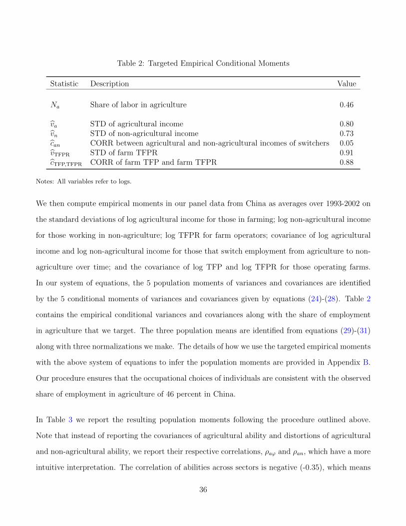
Table 2: Targeted Empirical Conditional Moments

Statistic Description Value

Na Share of labor in agriculture 0.46

va STD of agricultural income 0.80vn STD of non-agricultural income 0.73can CORR between agricultural and non-agricultural incomes of switchers 0.05vTFPR STD of farm TFPR 0.91cTFP,TFPR CORR of farm TFP and farm TFPR 0.88

Notes: All variables refer to logs.

We then compute empirical moments in our panel data from China as averages over 1993-2002 on

the standard deviations of log agricultural income for those in farming; log non-agricultural income

for those working in non-agriculture; log TFPR for farm operators; covariance of log agricultural

income and log non-agricultural income for those that switch employment from agriculture to non-

agriculture over time; and the covariance of log TFP and log TFPR for those operating farms.

In our system of equations, the 5 population moments of variances and covariances are identified

by the 5 conditional moments of variances and covariances given by equations (24)-(28). Table 2

contains the empirical conditional variances and covariances along with the share of employment

in agriculture that we target. The three population means are identified from equations (29)-(31)

along with three normalizations we make. The details of how we use the targeted empirical moments

with the above system of equations to infer the population moments are provided in Appendix B.

Our procedure ensures that the occupational choices of individuals are consistent with the observed

share of employment in agriculture of 46 percent in China.

In Table 3 we report the resulting population moments following the procedure outlined above.

Note that instead of reporting the covariances of agricultural ability and distortions of agricultural

and non-agricultural ability, we report their respective correlations, ρaϕ and ρan, which have a more

intuitive interpretation. The correlation of abilities across sectors is negative (-0.35), which means

36

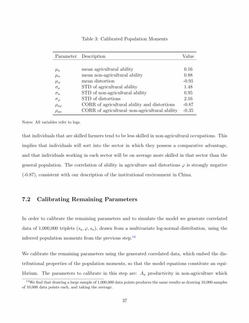
Table 3: Calibrated Population Moments

Parameter Description Value

µa mean agricultural ability 0.16µn mean non-agricultural ability 0.88µϕ mean distortion -0.91σa STD of agricultural ability 1.48σn STD of non-agricultural ability 0.95σϕ STD of distortions 2.16ρaϕ CORR of agricultural ability and distortions -0.87ρan CORR of agricultural–non-agricultural ability -0.35

Notes: All variables refer to logs.

that individuals that are skilled farmers tend to be less skilled in non-agricultural occupations. This

implies that individuals will sort into the sector in which they possess a comparative advantage,

and that individuals working in each sector will be on average more skilled in that sector than the

general population. The correlation of ability in agriculture and distortions ϕ is strongly negative

(-0.87), consistent with our description of the institutional environment in China.

7.2 Calibrating Remaining Parameters

In order to calibrate the remaining parameters and to simulate the model we generate correlated

data of 1,000,000 triplets (sa, ϕ, sn), drawn from a multivariate log-normal distribution, using the

inferred population moments from the previous step.14

We calibrate the remaining parameters using the generated correlated data, which embed the dis-

tributional properties of the population moments, so that the model equations constitute an equi-

librium. The parameters to calibrate in this step are: An productivity in non-agriculture which

14We find that drawing a large sample of 1,000,000 data points produces the same results as drawing 10,000 samplesof 10,000 data points each, and taking the average.

37

is normalized to 1; (α,γ) the elasticity parameters in the technology to produce the agricultural

good, which are set to α = 0.66 and γ = 0.54, following our analysis of measuring farm TFP and

misallocation in agriculture in Section 5; ω, the weight of the agricultural good in preferences, is set

to 0.01 to match a long run share of employment in agriculture of 1 percent; and the endowments

in agriculture of capital Ka and land L, are set to match a capital-output ratio in agriculture of 0.3

and an average farm size of 0.45 hectares, both as observed in our micro data. We normalize the

relative price of agriculture to 1 and solve the equilibrium of the model to obtain the subsistence

consumption of agricultural goods in preferences a to reproduce a share of employment in agricul-

ture of 46 percent and the productivity in agriculture Aa to match our definition of the common

term in agricultural income wa = 1 in equation (19). Table 4 displays the aggregate and micro-level

statistics for the benchmark economy, as well as the values for the calibrated parameters. The

model reproduces well the macro and micro statistics for China. Note for example that whereas

the static gain from efficient reallocation in the data is 84 percent, it is 66 percent in the model.

The difference arises mainly because the actual distributions of TFP and distortions in the data are

approximated in the model by a log-normal distribution.

8 Quantitative Experiments

We conduct a set of counterfactual experiments in order to assess the quantitative importance of

farm-specific distortions for the allocation of resources within agriculture, the sector-occupation

choices of individuals, as well as the amplification effect that selection imparts on sectoral produc-

tivity and real GDP per worker. We consider in turn: (a) the effects of eliminating farm-specific

distortions; (b) these effects compared to those from an exogenous increase in TFP; and (c) the

pattern of selection with sectoral reallocation.

38

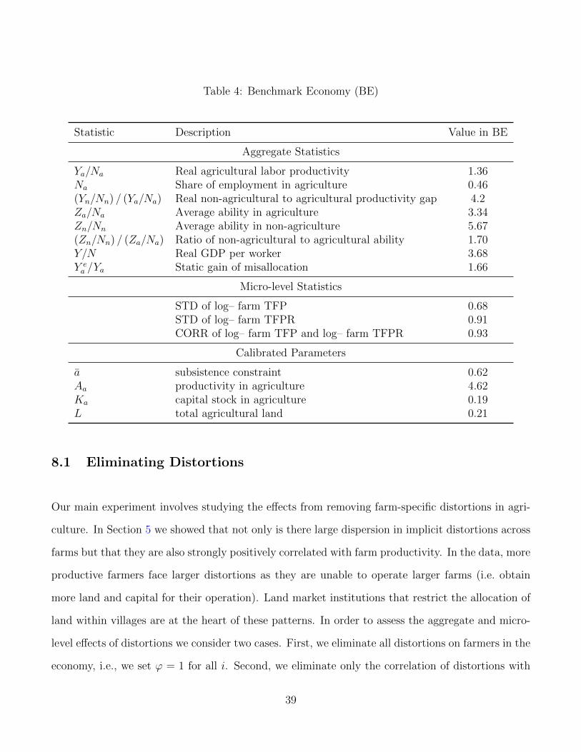
Table 4: Benchmark Economy (BE)

Statistic Description Value in BE

Aggregate Statistics

Ya/Na Real agricultural labor productivity 1.36Na Share of employment in agriculture 0.46(Yn/Nn) / (Ya/Na) Real non-agricultural to agricultural productivity gap 4.2Za/Na Average ability in agriculture 3.34Zn/Nn Average ability in non-agriculture 5.67(Zn/Nn) / (Za/Na) Ratio of non-agricultural to agricultural ability 1.70Y/N Real GDP per worker 3.68Y ea /Ya Static gain of misallocation 1.66

Micro-level Statistics

STD of log– farm TFP 0.68STD of log– farm TFPR 0.91CORR of log– farm TFP and log– farm TFPR 0.93

Calibrated Parameters

a subsistence constraint 0.62Aa productivity in agriculture 4.62Ka capital stock in agriculture 0.19L total agricultural land 0.21

8.1 Eliminating Distortions

Our main experiment involves studying the effects from removing farm-specific distortions in agri-

culture. In Section 5 we showed that not only is there large dispersion in implicit distortions across

farms but that they are also strongly positively correlated with farm productivity. In the data, more

productive farmers face larger distortions as they are unable to operate larger farms (i.e. obtain

more land and capital for their operation). Land market institutions that restrict the allocation of

land within villages are at the heart of these patterns. In order to assess the aggregate and micro-

level effects of distortions we consider two cases. First, we eliminate all distortions on farmers in the

economy, i.e., we set ϕ = 1 for all i. Second, we eliminate only the correlation of distortions with

39

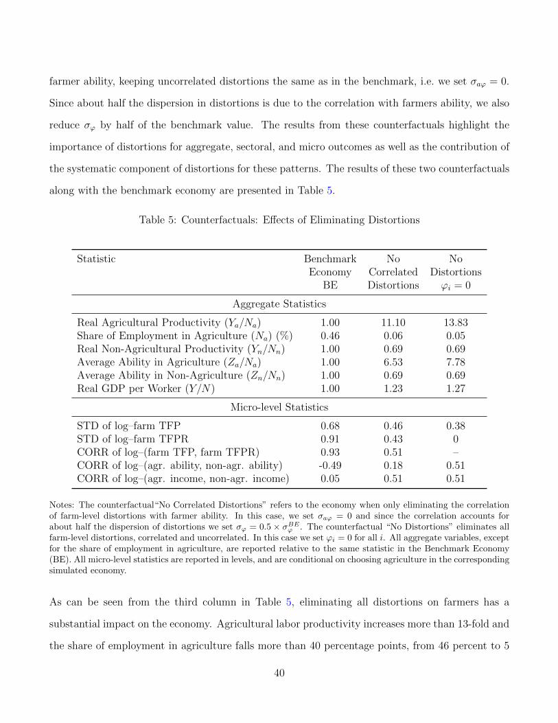
farmer ability, keeping uncorrelated distortions the same as in the benchmark, i.e. we set σaϕ = 0.

Since about half the dispersion in distortions is due to the correlation with farmers ability, we also

reduce σϕ by half of the benchmark value. The results from these counterfactuals highlight the

importance of distortions for aggregate, sectoral, and micro outcomes as well as the contribution of

the systematic component of distortions for these patterns. The results of these two counterfactuals

along with the benchmark economy are presented in Table 5.

Table 5: Counterfactuals: Effects of Eliminating Distortions

Statistic Benchmark No NoEconomy Correlated Distortions

BE Distortions ϕi = 0

Aggregate Statistics

Real Agricultural Productivity (Ya/Na) 1.00 11.10 13.83Share of Employment in Agriculture (Na) (%) 0.46 0.06 0.05Real Non-Agricultural Productivity (Yn/Nn) 1.00 0.69 0.69Average Ability in Agriculture (Za/Na) 1.00 6.53 7.78Average Ability in Non-Agriculture (Zn/Nn) 1.00 0.69 0.69Real GDP per Worker (Y/N) 1.00 1.23 1.27

Micro-level Statistics

STD of log–farm TFP 0.68 0.46 0.38STD of log–farm TFPR 0.91 0.43 0CORR of log–(farm TFP, farm TFPR) 0.93 0.51 –CORR of log–(agr. ability, non-agr. ability) -0.49 0.18 0.51CORR of log–(agr. income, non-agr. income) 0.05 0.51 0.51

Notes: The counterfactual“No Correlated Distortions” refers to the economy when only eliminating the correlationof farm-level distortions with farmer ability. In this case, we set σaϕ = 0 and since the correlation accounts forabout half the dispersion of distortions we set σϕ = 0.5 × σBEϕ . The counterfactual “No Distortions” eliminates allfarm-level distortions, correlated and uncorrelated. In this case we set ϕi = 0 for all i. All aggregate variables, exceptfor the share of employment in agriculture, are reported relative to the same statistic in the Benchmark Economy(BE). All micro-level statistics are reported in levels, and are conditional on choosing agriculture in the correspondingsimulated economy.

As can be seen from the third column in Table 5, eliminating all distortions on farmers has a

substantial impact on the economy. Agricultural labor productivity increases more than 13-fold and

the share of employment in agriculture falls more than 40 percentage points, from 46 percent to 5

40

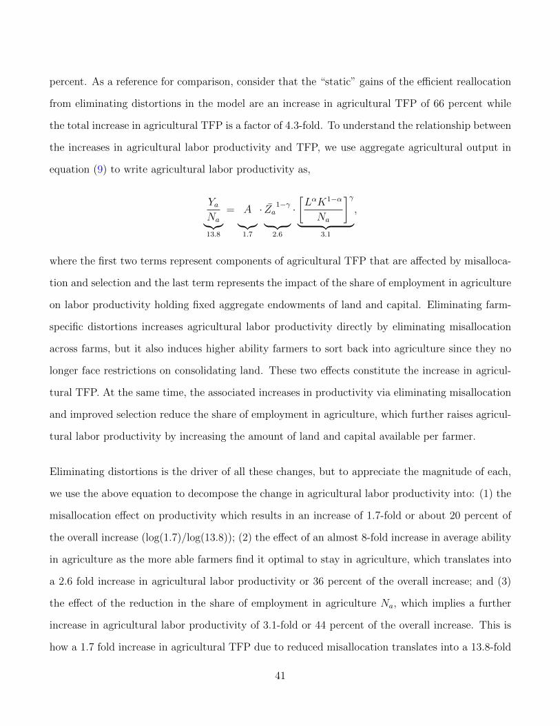
percent. As a reference for comparison, consider that the “static” gains of the efficient reallocation

from eliminating distortions in the model are an increase in agricultural TFP of 66 percent while

the total increase in agricultural TFP is a factor of 4.3-fold. To understand the relationship between

the increases in agricultural labor productivity and TFP, we use aggregate agricultural output in

equation (9) to write agricultural labor productivity as,

YaNa︸︷︷︸13.8

= A︸︷︷︸1.7

· Za1−γ

︸ ︷︷ ︸2.6

·[LαK1−α

Na

]γ︸ ︷︷ ︸

3.1

,

where the first two terms represent components of agricultural TFP that are affected by misalloca-

tion and selection and the last term represents the impact of the share of employment in agriculture

on labor productivity holding fixed aggregate endowments of land and capital. Eliminating farm-

specific distortions increases agricultural labor productivity directly by eliminating misallocation

across farms, but it also induces higher ability farmers to sort back into agriculture since they no

longer face restrictions on consolidating land. These two effects constitute the increase in agricul-

tural TFP. At the same time, the associated increases in productivity via eliminating misallocation

and improved selection reduce the share of employment in agriculture, which further raises agricul-

tural labor productivity by increasing the amount of land and capital available per farmer.

Eliminating distortions is the driver of all these changes, but to appreciate the magnitude of each,

we use the above equation to decompose the change in agricultural labor productivity into: (1) the

misallocation effect on productivity which results in an increase of 1.7-fold or about 20 percent of

the overall increase (log(1.7)/log(13.8)); (2) the effect of an almost 8-fold increase in average ability

in agriculture as the more able farmers find it optimal to stay in agriculture, which translates into

a 2.6 fold increase in agricultural labor productivity or 36 percent of the overall increase; and (3)

the effect of the reduction in the share of employment in agriculture Na, which implies a further

increase in agricultural labor productivity of 3.1-fold or 44 percent of the overall increase. This is

how a 1.7 fold increase in agricultural TFP due to reduced misallocation translates into a 13.8-fold

41

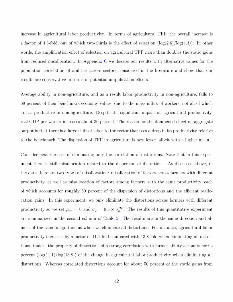
increase in agricultural labor productivity. In terms of agricultural TFP, the overall increase is

a factor of 4.3-fold, out of which two-thirds is the effect of selection (log(2.6)/log(4.3)). In other

words, the amplification effect of selection on agricultural TFP more than doubles the static gains

from reduced misallocation. In Appendix C we discuss our results with alternative values for the

population correlation of abilities across sectors considered in the literature and show that our

results are conservative in terms of potential amplification effects.

Average ability in non-agriculture, and as a result labor productivity in non-agriculture, falls to

69 percent of their benchmark economy values, due to the mass influx of workers, not all of which

are as productive in non-agriculture. Despite the significant impact on agricultural productivity,

real GDP per worker increases about 30 percent. The reason for the dampened effect on aggregate

output is that there is a large shift of labor to the sector that sees a drop in its productivity relative

to the benchmark. The dispersion of TFP in agriculture is now lower, albeit with a higher mean.

Consider next the case of eliminating only the correlation of distortions. Note that in this exper-

iment there is still misallocation related to the dispersion of distortions. As discussed above, in

the data there are two types of misallocation: misallocation of factors across farmers with different

productivity, as well as misallocation of factors among farmers with the same productivity, each

of which accounts for roughly 50 percent of the dispersion of distortions and the efficient reallo-

cation gains. In this experiment, we only eliminate the distortions across farmers with different

productivity so we set ρaϕ = 0 and σϕ = 0.5 × σBEϕ . The results of this quantitative experiment

are summarized in the second column of Table 5. The results are in the same direction and al-

most of the same magnitude as when we eliminate all distortions. For instance, agricultural labor

productivity increases by a factor of 11.1-fold compared with 13.8-fold when eliminating all distor-

tions, that is, the property of distortions of a strong correlation with farmer ability accounts for 92

percent (log(11.1)/log(13.8)) of the change in agricultural labor productivity when eliminating all

distortions. Whereas correlated distortions account for about 50 percent of the static gains from

42

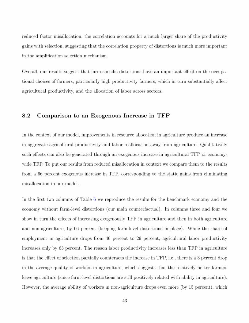
reduced factor misallocation, the correlation accounts for a much larger share of the productivity

gains with selection, suggesting that the correlation property of distortions is much more important

in the amplification selection mechanism.

Overall, our results suggest that farm-specific distortions have an important effect on the occupa-

tional choices of farmers, particularly high productivity farmers, which in turn substantially affect

agricultural productivity, and the allocation of labor across sectors.

8.2 Comparison to an Exogenous Increase in TFP

In the context of our model, improvements in resource allocation in agriculture produce an increase

in aggregate agricultural productivity and labor reallocation away from agriculture. Qualitatively

such effects can also be generated through an exogenous increase in agricultural TFP or economy-

wide TFP. To put our results from reduced misallocation in context we compare them to the results

from a 66 percent exogenous increase in TFP, corresponding to the static gains from eliminating

misallocation in our model.

In the first two columns of Table 6 we reproduce the results for the benchmark economy and the

economy without farm-level distortions (our main counterfactual). In columns three and four we

show in turn the effects of increasing exogenously TFP in agriculture and then in both agriculture

and non-agriculture, by 66 percent (keeping farm-level distortions in place). While the share of

employment in agriculture drops from 46 percent to 29 percent, agricultural labor productivity

increases only by 63 percent. The reason labor productivity increases less than TFP in agriculture

is that the effect of selection partially counteracts the increase in TFP, i.e., there is a 3 percent drop

in the average quality of workers in agriculture, which suggests that the relatively better farmers

leave agriculture (since farm-level distortions are still positively related with ability in agriculture).

However, the average ability of workers in non-agriculture drops even more (by 15 percent), which

43

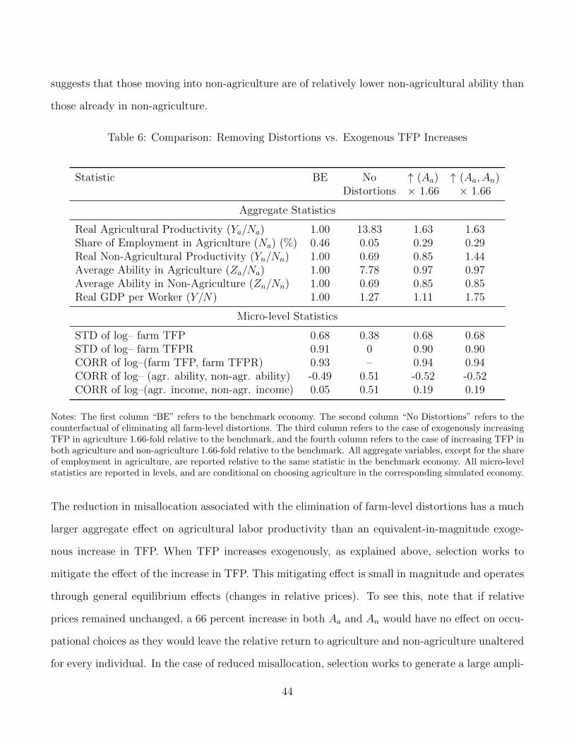
suggests that those moving into non-agriculture are of relatively lower non-agricultural ability than

those already in non-agriculture.

Table 6: Comparison: Removing Distortions vs. Exogenous TFP Increases

Statistic BE No ↑ (Aa) ↑ (Aa, An)Distortions × 1.66 × 1.66

Aggregate Statistics

Real Agricultural Productivity (Ya/Na) 1.00 13.83 1.63 1.63Share of Employment in Agriculture (Na) (%) 0.46 0.05 0.29 0.29Real Non-Agricultural Productivity (Yn/Nn) 1.00 0.69 0.85 1.44Average Ability in Agriculture (Za/Na) 1.00 7.78 0.97 0.97Average Ability in Non-Agriculture (Zn/Nn) 1.00 0.69 0.85 0.85Real GDP per Worker (Y/N) 1.00 1.27 1.11 1.75

Micro-level Statistics

STD of log– farm TFP 0.68 0.38 0.68 0.68STD of log– farm TFPR 0.91 0 0.90 0.90CORR of log–(farm TFP, farm TFPR) 0.93 – 0.94 0.94CORR of log– (agr. ability, non-agr. ability) -0.49 0.51 -0.52 -0.52CORR of log–(agr. income, non-agr. income) 0.05 0.51 0.19 0.19

Notes: The first column “BE” refers to the benchmark economy. The second column “No Distortions” refers to thecounterfactual of eliminating all farm-level distortions. The third column refers to the case of exogenously increasingTFP in agriculture 1.66-fold relative to the benchmark, and the fourth column refers to the case of increasing TFP inboth agriculture and non-agriculture 1.66-fold relative to the benchmark. All aggregate variables, except for the shareof employment in agriculture, are reported relative to the same statistic in the benchmark economy. All micro-levelstatistics are reported in levels, and are conditional on choosing agriculture in the corresponding simulated economy.

The reduction in misallocation associated with the elimination of farm-level distortions has a much

larger aggregate effect on agricultural labor productivity than an equivalent-in-magnitude exoge-

nous increase in TFP. When TFP increases exogenously, as explained above, selection works to

mitigate the effect of the increase in TFP. This mitigating effect is small in magnitude and operates

through general equilibrium effects (changes in relative prices). To see this, note that if relative

prices remained unchanged, a 66 percent increase in both Aa and An would have no effect on occu-

pational choices as they would leave the relative return to agriculture and non-agriculture unaltered

for every individual. In the case of reduced misallocation, selection works to generate a large ampli-

44

fication effect on agricultural labor productivity, over and above the static misallocation gains of 66

percent. The reason for this is that farm-level distortions directly impact the occupational choices

of individuals, particularly the high agricultural ability ones. Removing farm-level distortions alters

the pattern of occupational choices of individuals even holding constant aggregate prices.

This result is important as a challenge in the literature is to find measurable drivers of sectoral

reallocation and increased productivity in agriculture relative to non-agriculture. In an important

contribution, Lagakos and Waugh (2013) highlighted selection as a substantial amplification mech-

anism of productivity differences, an insight we build on in our paper. But as emphasized in our

results, reasonable economy-wide productivity differences are unlikely to generate differences in

sectoral reallocation and selection large enough to explain the large real sectoral productivity gaps

across rich and poor countries. We provide a measure of idiosyncratic distortions in agriculture as

a specific and distinct driver of sectoral reallocation that has a strong effect on occupational choices

and selection, generating both a direct effect on agricultural productivity and an amplification ef-

fect that is orders of magnitude larger than the effect from aggregate distortions or economy-wide

productivity differences.

8.3 Sectoral Reallocation and Selection Patterns

Our empirical findings indicate that farm-level distortions have not changed much over the period

we examine, consistent with the unchanged land-market institutions in China. Yet in the data

we observe that households are moving out of agriculture and into non-agriculture at a rate of

about 1 percent per year. This occurs because the economy grows even with farm-level distortions.

Non-agricultural labor productivity increases 7 percent per year over the period we examine, with

an overall increase of 97 percent over 1993-2002. In Table 7 we show what happens in the bench-

mark economy in the presence of the observed farm-level distortions when TFP increases in both

45

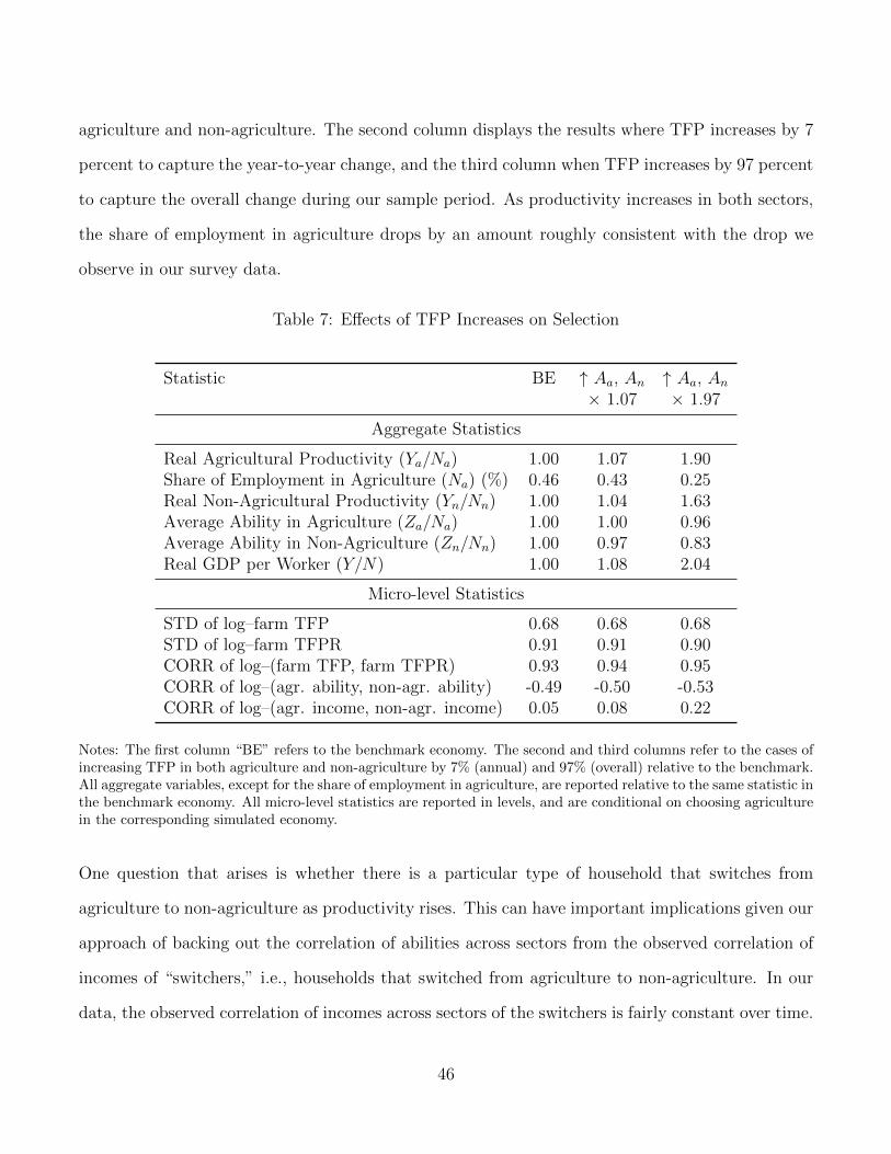
agriculture and non-agriculture. The second column displays the results where TFP increases by 7

percent to capture the year-to-year change, and the third column when TFP increases by 97 percent

to capture the overall change during our sample period. As productivity increases in both sectors,

the share of employment in agriculture drops by an amount roughly consistent with the drop we

observe in our survey data.

Table 7: Effects of TFP Increases on Selection

Statistic BE ↑ Aa, An ↑ Aa, An× 1.07 × 1.97

Aggregate Statistics

Real Agricultural Productivity (Ya/Na) 1.00 1.07 1.90Share of Employment in Agriculture (Na) (%) 0.46 0.43 0.25Real Non-Agricultural Productivity (Yn/Nn) 1.00 1.04 1.63Average Ability in Agriculture (Za/Na) 1.00 1.00 0.96Average Ability in Non-Agriculture (Zn/Nn) 1.00 0.97 0.83Real GDP per Worker (Y/N) 1.00 1.08 2.04

Micro-level Statistics

STD of log–farm TFP 0.68 0.68 0.68STD of log–farm TFPR 0.91 0.91 0.90CORR of log–(farm TFP, farm TFPR) 0.93 0.94 0.95CORR of log–(agr. ability, non-agr. ability) -0.49 -0.50 -0.53CORR of log–(agr. income, non-agr. income) 0.05 0.08 0.22

Notes: The first column “BE” refers to the benchmark economy. The second and third columns refer to the cases ofincreasing TFP in both agriculture and non-agriculture by 7% (annual) and 97% (overall) relative to the benchmark.All aggregate variables, except for the share of employment in agriculture, are reported relative to the same statistic inthe benchmark economy. All micro-level statistics are reported in levels, and are conditional on choosing agriculturein the corresponding simulated economy.

One question that arises is whether there is a particular type of household that switches from

agriculture to non-agriculture as productivity rises. This can have important implications given our

approach of backing out the correlation of abilities across sectors from the observed correlation of

incomes of “switchers,” i.e., households that switched from agriculture to non-agriculture. In our

data, the observed correlation of incomes across sectors of the switchers is fairly constant over time.

46

The question though is whether this correlation is biased because of the type of households that in

fact switch. We examine this question in the context of our model by considering the micro-level

implications of exogenous increases in TFP, and in particular the implications for the correlation

of abilities and the correlation of incomes across sectors, in turn, as the share of individuals in

agriculture drops. The results of Table 7 indicate that for year-to-year changes (second column)

the correlation of agricultural and non-agricultural abilities across sectors and the corresponding

correlation of incomes are largely unchanged. Over the entire period (third column), the correlation

of abilities again exhibits little change, while the correlation of incomes increases more. These

changes however are roughly consistent with the range of changes observed in the data. These

results suggest that the bulk of changes in sectoral reallocation in China during the sample period

are driven by changes in non-agricultural labor productivity and not so much by changes in the

agricultural distortions associated with the land market institutions and the “hukou” system.

While eliminating distortions leads to a substantial increase in agricultural labor productivity (13.8-

fold), aggregate GDP per worker increases by only 27 percent. The reason is that there is a massive

shift of labor from agriculture to non-agriculture, a sector that sees a drop in its productivity (by

about 30 percent). In reality however non-agricultural labor productivity increases by 97 percent

over the period we examine. Taking this into account, the effect on real GDP per worker from

eliminating distortions is more pronounced, with aggregate real GDP per worker increasing 2.3-fold

(vs. 1.3-fold with just reduced misallocation). The reason is that with an increase in non-agricultural

TFP, non-agricultural labor productivity rises overall (from 0.69 when only eliminating distortions

to 1.37 when also increasing non-agricultural productivity), despite the negative selection effect

operating on it. The micro-level implications of the economy without distortions and the economy

without distortions and an exogenous rise in TFP are identical. In a growing economy, eliminating

farm-level distortions can translate into significant aggregate productivity growth.

47

9 Conclusions

Using a simple quantitative framework and micro panel data, we presented evidence that capital

and land are severely misallocated across farmers in China. Given the institutional framework,

we argued that this factor misallocation reflects primarily restrictions in the land market, which

also dampen access to credit for farmers. The administrative allocation of land-use rights on an

egalitarian basis manifests itself as a larger idiosyncratic distortion on the more productive farmers.

In addition, the resulting pattern of misallocation shows no systematic tendency to improve over

time, consistent with the persistent nature of the institutional restrictions in the Chinese economy.

Using the idiosyncratic distortions we measure across farmers in China, we develop and estimate

a two-sector general-equilibrium model of occupational selection. The panel data provide us with

information on income in agriculture and wages in non-agriculture for individuals that switch occu-

pations, which we use to restrict the correlation of abilities across sectors in the population. We find

that measured distortions substantially affect the observed distribution of farm TFP in the Chi-

nese data, and that eliminating the correlation of these distortions with farmer’s ability improves

aggregate agricultural productivity via reduced misallocation and improved selection of more able

farmers into agriculture. This effect substantially contributes to structural change and growth.

Our analysis implies that implementing a system of secure property rights to facilitate a decen-

tralized allocation of land would generate large aggregate productivity gains. To the extent that

village officials do not observe farmer ability or do not make land allocation decisions based on

ability, any administrative (re)allocation of land would be unable to channel land to farmers that

value it the most or can make the most out of it. Developing a market allocation mechanism by

extending fully transferable use rights over land to farmers will not only allow farmers to increase

their operational scales through land consolidations, but would also induce the best farmers to stay

in agriculture, while releasing labor to non-agriculture. The productivity and farm size increases

48

due to a better allocation of factors of production among farmers and an improved selection of

farmers in agriculture can arguably also induce changes in farm operations by incentivizing farmers

to use modern inputs and better technologies. We leave this important extension of our framework

for future research.

References

Adamopoulos, T. and Restuccia, D. (2014). The Size Distribution of Farms and InternationalProductivity Differences. American Economic Review, 104(6):1667–97.

Adamopoulos, T. and Restuccia, D. (2015). Land Reform and Productivity: A Quantitative Anal-ysis with Micro Data.

Benjamin, D. and Brandt, L. (2002). Property rights, labour markets, and efficiency in a transitioneconomy: the case of rural china. Canadian Journal of Economics, pages 689–716.

Benjamin, D., Brandt, L., and Giles, J. (2005). The evolution of income inequality in rural china.Economic Development and Cultural Change, 53(4):769–824.

Brandt, L., Huang, J., Li, G., and Rozelle, S. (2002). Land rights in rural china: Facts, fictions andissues. The China Journal, (47):67–97.

Brandt, L., Tombe, T., and Zhu, X. (2013). Factor market distortions across time, space and sectorsin china. Review of Economic Dynamics, 16(1):39–58.

Chen, C. (2016). Untitled Land, Occupational Choice and Agricultural Productivity. AmericanEconomic Journal: Macroeconomics, forthcoming.

de Janvry, A., Emerick, K., Gonzalez-Navarro, M., and Sadoulet, E. (2014). Delinking land rightsfrom land use: Certification and migration in mexico.

Gollin, D., Parente, S., and Rogerson, R. (2002). The Role of Agriculture in Development. AmericanEconomic Review, 92(2):160–164.

Gottlieb, C. and Grobovsek, J. (2015). Communal Land and Agricultural Productivity,. Unpub-lished manuscript, University of Edinburgh.

Hsieh, C.-T. and Klenow, P. J. (2009). Misallocation and Manufacturing TFP in China and India.The Quarterly Journal of Economics, 124(4):1403–1448.

Kung, J. K.-s. and Liu, S. (1997). Farmers’ preferences regarding ownership and land tenure inpost-mao china: unexpected evidence from eight counties. The China Journal, (38):33–63.

49

Lagakos, D. and Waugh, M. E. (2013). Selection, agriculture, and cross-country productivitydifferences. The American Economic Review, 103(2):948–980.

Lin, J. Y. (1992). Rural reforms and agricultural growth in china. The American Economic Review,pages 34–51.

Lucas Jr, R. E. (1978). On the size distribution of business firms. The Bell Journal of Economics,pages 508–523.

McMillan, J., Whalley, J., and Zhu, L. (1989). The impact of china’s economic reforms on agricul-tural productivity growth. The Journal of Political Economy, pages 781–807.

Ngai, R., Pissarides, C., and Wang, J. (2016). Chinas mobility barriers and employment allocations.Technical report.

Restuccia, D. and Rogerson, R. (2008). Policy Distortions and Aggregate Productivity with Het-erogeneous Plants. Review of Economic Dynamics, 11(4):707–720.

Restuccia, D. and Rogerson, R. (2013). Misallocation and Productivity. Review of EconomicDynamics, 16(1):1–10.

Restuccia, D. and Rogerson, R. (2016). The causes and costs of misallocation. Unpublishedmanuscript, University of Toronto.

Restuccia, D. and Santaeulalia-Llopis, R. (2015). Land misallocation and productivity. Unpublishedmanuscript, University of Toronto.

Restuccia, D., Yang, D. T., and Zhu, X. (2008). Agriculture and aggregate productivity: A quan-titative cross-country analysis. Journal of Monetary Economics, 55(2):234–250.

Roy, A. D. (1951). Some thoughts on the distribution of earnings. Oxford economic papers, 3(2):135–146.

Song, Z., Storesletten, K., and Zilibotti, F. (2011). Growing like china. The American EconomicReview, 101(1):196–233.

Tombe, T. and Zhu, X. (2015). Trade, migration and productivity: A quantitative analysis of china.Technical report.

Yang, D. T. (1997). China’s land arrangements and rural labor mobility. China Economic Review,8(2):101–115.

Zhu, X. (2012). Understanding chinas growth: Past, present, and future (digest summary). Journalof Economic Perspectives, 26(4):103–124.

50

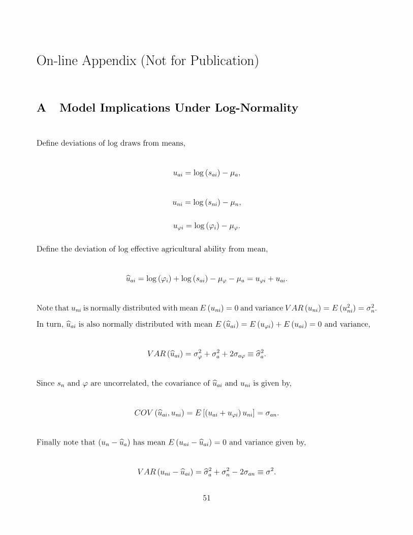
On-line Appendix (Not for Publication)

A Model Implications Under Log-Normality

Define deviations of log draws from means,

uai = log (sai)− µa,

uni = log (sni)− µn,

uϕi = log (ϕi)− µϕ.

Define the deviation of log effective agricultural ability from mean,

uai = log (ϕi) + log (sai)− µϕ − µa = uϕi + uai.

Note that uni is normally distributed with mean E (uni) = 0 and variance V AR (uni) = E (u2ni) = σ2n.

In turn, uai is also normally distributed with mean E (uai) = E (uϕi) + E (uai) = 0 and variance,

V AR (uai) = σ2ϕ + σ2

a + 2σaϕ ≡ σ2a.

Since sn and ϕ are uncorrelated, the covariance of uai and uni is given by,

COV (uai, uni) = E [(uai + uϕi)uni] = σan.

Finally note that (un − ua) has mean E (uni − uai) = 0 and variance given by,

V AR (uni − uai) = σ2a + σ2

n − 2σan ≡ σ2.

51

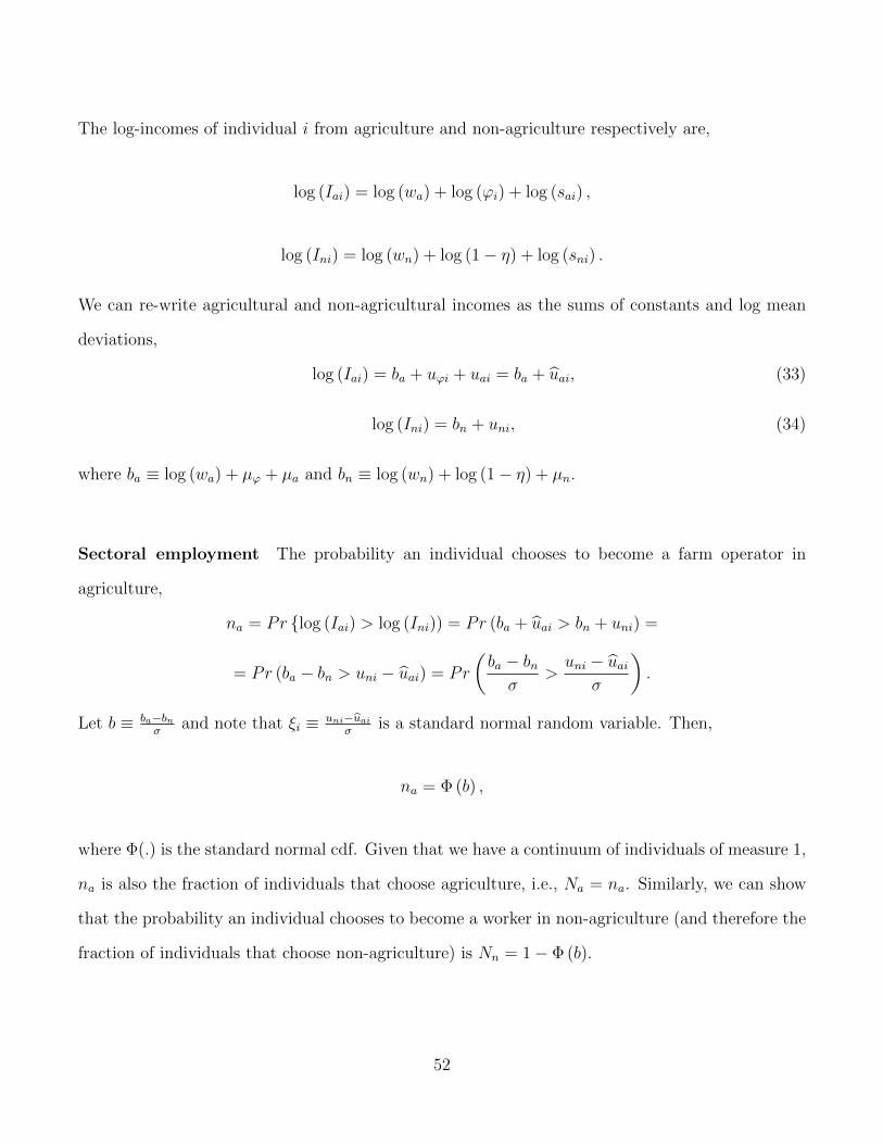
The log-incomes of individual i from agriculture and non-agriculture respectively are,

log (Iai) = log (wa) + log (ϕi) + log (sai) ,

log (Ini) = log (wn) + log (1− η) + log (sni) .

We can re-write agricultural and non-agricultural incomes as the sums of constants and log mean

deviations,

log (Iai) = ba + uϕi + uai = ba + uai, (33)

log (Ini) = bn + uni, (34)

where ba ≡ log (wa) + µϕ + µa and bn ≡ log (wn) + log (1− η) + µn.

Sectoral employment The probability an individual chooses to become a farm operator in

agriculture,

na = Pr {log (Iai) > log (Ini)) = Pr (ba + uai > bn + uni) =

= Pr (ba − bn > uni − uai) = Pr

(ba − bnσ

>uni − uai

σ

).

Let b ≡ ba−bnσ

and note that ξi ≡ uni−uaiσ

is a standard normal random variable. Then,

na = Φ (b) ,

where Φ(.) is the standard normal cdf. Given that we have a continuum of individuals of measure 1,

na is also the fraction of individuals that choose agriculture, i.e., Na = na. Similarly, we can show

that the probability an individual chooses to become a worker in non-agriculture (and therefore the

fraction of individuals that choose non-agriculture) is Nn = 1− Φ (b).

52

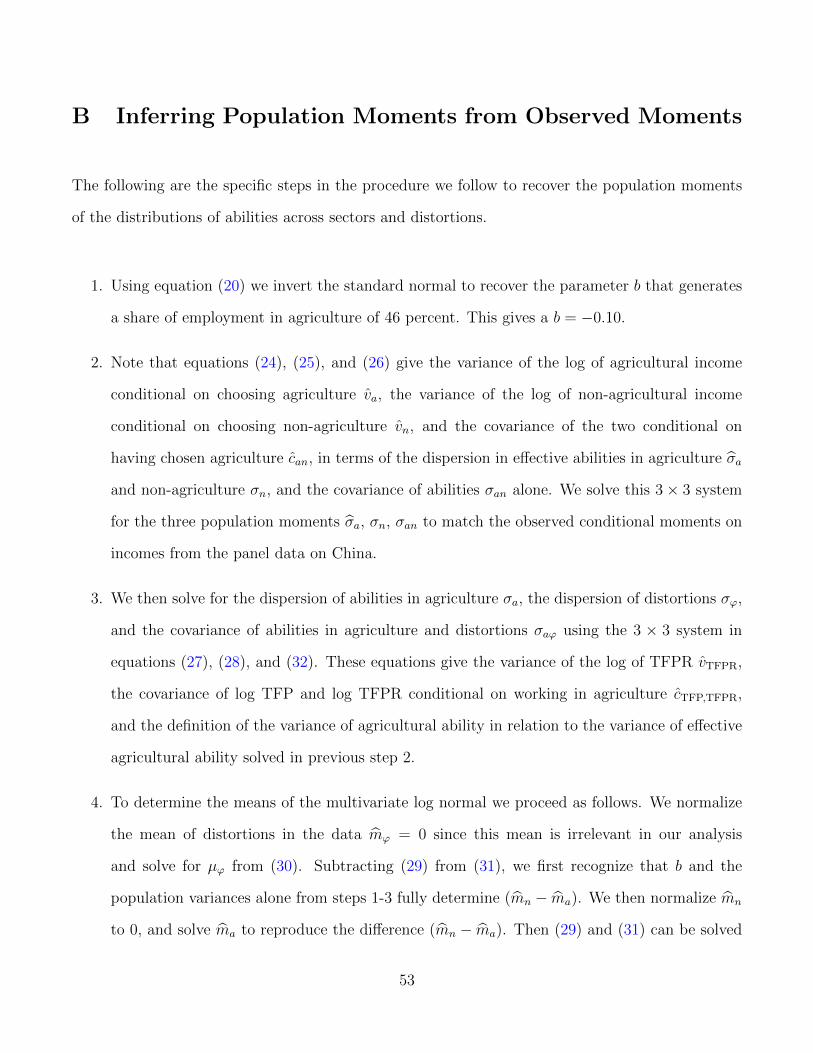
B Inferring Population Moments from Observed Moments

The following are the specific steps in the procedure we follow to recover the population moments

of the distributions of abilities across sectors and distortions.

1. Using equation (20) we invert the standard normal to recover the parameter b that generates

a share of employment in agriculture of 46 percent. This gives a b = −0.10.

2. Note that equations (24), (25), and (26) give the variance of the log of agricultural income

conditional on choosing agriculture va, the variance of the log of non-agricultural income

conditional on choosing non-agriculture vn, and the covariance of the two conditional on

having chosen agriculture can, in terms of the dispersion in effective abilities in agriculture σa

and non-agriculture σn, and the covariance of abilities σan alone. We solve this 3× 3 system

for the three population moments σa, σn, σan to match the observed conditional moments on

incomes from the panel data on China.

3. We then solve for the dispersion of abilities in agriculture σa, the dispersion of distortions σϕ,

and the covariance of abilities in agriculture and distortions σaϕ using the 3 × 3 system in

equations (27), (28), and (32). These equations give the variance of the log of TFPR vTFPR,

the covariance of log TFP and log TFPR conditional on working in agriculture cTFP,TFPR,

and the definition of the variance of agricultural ability in relation to the variance of effective

agricultural ability solved in previous step 2.

4. To determine the means of the multivariate log normal we proceed as follows. We normalize

the mean of distortions in the data mϕ = 0 since this mean is irrelevant in our analysis

and solve for µϕ from (30). Subtracting (29) from (31), we first recognize that b and the

population variances alone from steps 1-3 fully determine (mn − ma). We then normalize mn

to 0, and solve ma to reproduce the difference (mn − ma). Then (29) and (31) can be solved

53

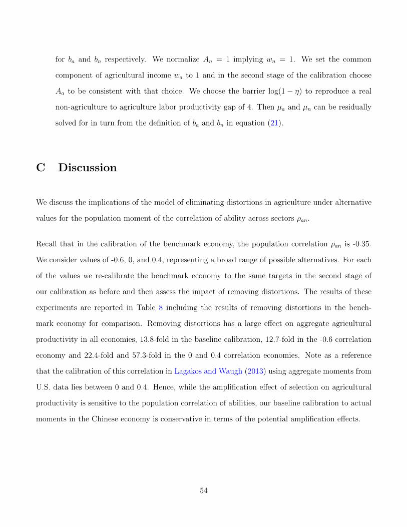
for ba and bn respectively. We normalize An = 1 implying wn = 1. We set the common

component of agricultural income wa to 1 and in the second stage of the calibration choose

Aa to be consistent with that choice. We choose the barrier log(1− η) to reproduce a real

non-agriculture to agriculture labor productivity gap of 4. Then µa and µn can be residually

solved for in turn from the definition of ba and bn in equation (21).

C Discussion

We discuss the implications of the model of eliminating distortions in agriculture under alternative

values for the population moment of the correlation of ability across sectors ρan.

Recall that in the calibration of the benchmark economy, the population correlation ρan is -0.35.

We consider values of -0.6, 0, and 0.4, representing a broad range of possible alternatives. For each

of the values we re-calibrate the benchmark economy to the same targets in the second stage of

our calibration as before and then assess the impact of removing distortions. The results of these

experiments are reported in Table 8 including the results of removing distortions in the bench-

mark economy for comparison. Removing distortions has a large effect on aggregate agricultural

productivity in all economies, 13.8-fold in the baseline calibration, 12.7-fold in the -0.6 correlation

economy and 22.4-fold and 57.3-fold in the 0 and 0.4 correlation economies. Note as a reference

that the calibration of this correlation in Lagakos and Waugh (2013) using aggregate moments from

U.S. data lies between 0 and 0.4. Hence, while the amplification effect of selection on agricultural

productivity is sensitive to the population correlation of abilities, our baseline calibration to actual

moments in the Chinese economy is conservative in terms of the potential amplification effects.

54

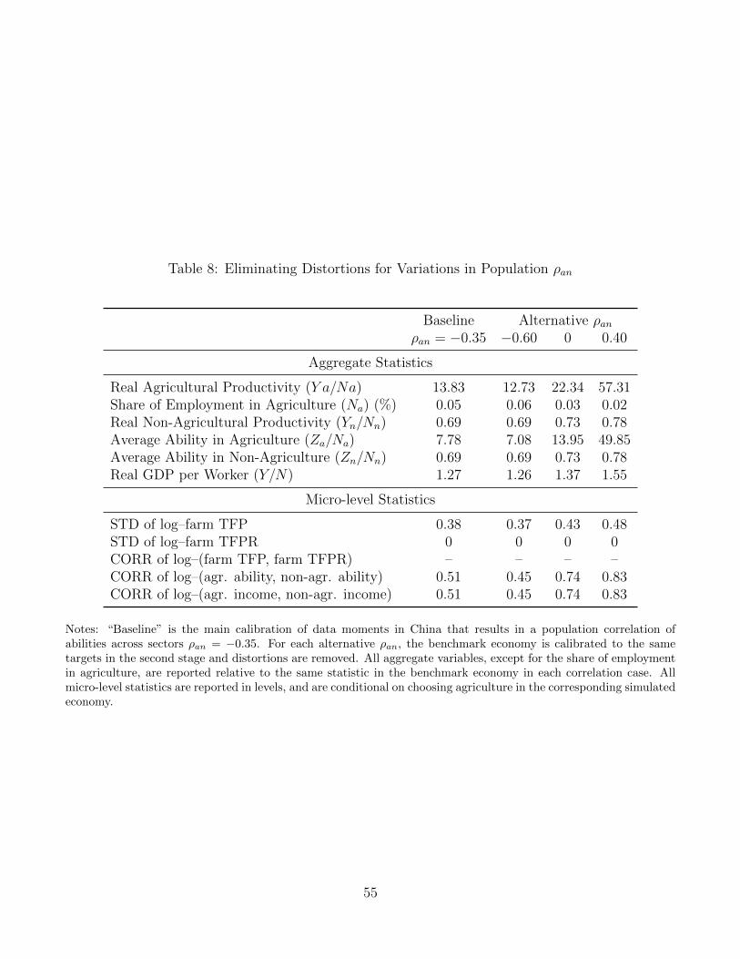
Table 8: Eliminating Distortions for Variations in Population ρan

Baseline Alternative ρanρan = −0.35 −0.60 0 0.40

Aggregate Statistics

Real Agricultural Productivity (Y a/Na) 13.83 12.73 22.34 57.31Share of Employment in Agriculture (Na) (%) 0.05 0.06 0.03 0.02Real Non-Agricultural Productivity (Yn/Nn) 0.69 0.69 0.73 0.78Average Ability in Agriculture (Za/Na) 7.78 7.08 13.95 49.85Average Ability in Non-Agriculture (Zn/Nn) 0.69 0.69 0.73 0.78Real GDP per Worker (Y/N) 1.27 1.26 1.37 1.55

Micro-level Statistics

STD of log–farm TFP 0.38 0.37 0.43 0.48STD of log–farm TFPR 0 0 0 0CORR of log–(farm TFP, farm TFPR) – – – –CORR of log–(agr. ability, non-agr. ability) 0.51 0.45 0.74 0.83CORR of log–(agr. income, non-agr. income) 0.51 0.45 0.74 0.83

Notes: “Baseline” is the main calibration of data moments in China that results in a population correlation ofabilities across sectors ρan = −0.35. For each alternative ρan, the benchmark economy is calibrated to the sametargets in the second stage and distortions are removed. All aggregate variables, except for the share of employmentin agriculture, are reported relative to the same statistic in the benchmark economy in each correlation case. Allmicro-level statistics are reported in levels, and are conditional on choosing agriculture in the corresponding simulatedeconomy.

55