One-Shot Hyperspectral Imaging Using Faced...
9
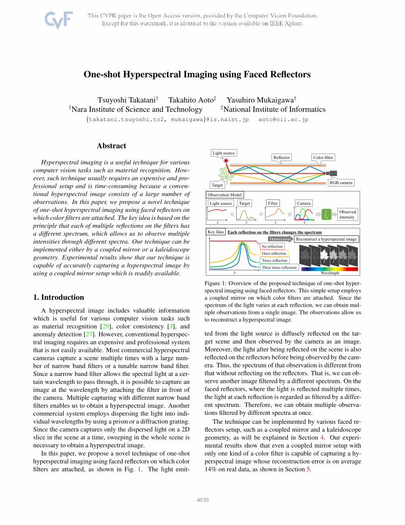
One-shot Hyperspectral Imaging using Faced Reflectors Tsuyoshi Takatani † Takahito Aoto ‡ Yasuhiro Mukaigawa † † Nara Institute of Science and Technology ‡ National Institute of Informatics {takatani.tsuyoshi.to2, mukaigawa}@is.naist.jp [email protected] Abstract Hyperspectral imaging is a useful technique for various computer vision tasks such as material recognition. How- ever, such technique usually requires an expensive and pro- fessional setup and is time-consuming because a conven- tional hyperspectral image consists of a large number of observations. In this paper, we propose a novel technique of one-shot hyperspectral imaging using faced reflectors on which color filters are attached. The key idea is based on the principle that each of multiple reflections on the filters has a different spectrum, which allows us to observe multiple intensities through different spectra. Our technique can be implemented either by a coupled mirror or a kaleidoscope geometry. Experimental results show that our technique is capable of accurately capturing a hyperspectral image by using a coupled mirror setup which is readily available. 1. Introduction A hyperspectral image includes valuable information which is useful for various computer vision tasks such as material recognition [29], color consistency [3], and anomaly detection [27]. However, conventional hyperspec- tral imaging requires an expensive and professional system that is not easily available. Most commercial hyperspectral cameras capture a scene multiple times with a large num- ber of narrow band filters or a tunable narrow band filter. Since a narrow band filter allows the spectral light at a cer- tain wavelength to pass through, it is possible to capture an image at the wavelength by attaching the filter in front of the camera. Multiple capturing with different narrow band filters enables us to obtain a hyperspectral image. Another commercial system employs dispersing the light into indi- vidual wavelengths by using a prism or a diffraction grating. Since the camera captures only the dispersed light on a 2D slice in the scene at a time, sweeping in the whole scene is necessary to obtain a hyperspectral image. In this paper, we propose a novel technique of one-shot hyperspectral imaging using faced reflectors on which color filters are attached, as shown in Fig. 1. The light emit- Light source RGB camera Target Reflector Color filter Observed intensity න Λ . Observation Model Light source Target Filter Camera Key Idea Each reflection on the filters changes the spectrum No reflection Once reflection Twice reflection Three times reflection Optimization Reconstruct a hyperspectral image Wavelength Figure 1: Overview of the proposed technique of one-shot hyper- spectral imaging using faced reflectors. This simple setup employs a coupled mirror on which color filters are attached. Since the spectrum of the light varies at each reflection, we can obtain mul- tiple observations from a single image. The observations allow us to reconstruct a hyperspectral image. ted from the light source is diffusely reflected on the tar- get scene and then observed by the camera as an image. Moreover, the light after being reflected on the scene is also reflected on the reflectors before being observed by the cam- era. Thus, the spectrum of that observation is different from that without reflecting on the reflectors. That is, we can ob- serve another image filtered by a different spectrum. On the faced reflectors, where the light is reflected multiple times, the light at each reflection is regarded as filtered by a differ- ent spectrum. Therefore, we can obtain multiple observa- tions filtered by different spectra at once. The technique can be implemented by various faced re- flectors setup, such as a coupled mirror and a kaleidoscope geometry, as will be explained in Section 4. Our experi- mental results show that even a coupled mirror setup with only one kind of a color filter is capable of capturing a hy- perspectral image whose reconstruction error is on average 14% on real data, as shown in Section 5. 4039
Transcript of One-Shot Hyperspectral Imaging Using Faced...
One-shot Hyperspectral Imaging using Faced Reflectors
Tsuyoshi Takatani† Takahito Aoto‡ Yasuhiro Mukaigawa††Nara Institute of Science and Technology ‡National Institute of Informatics
{takatani.tsuyoshi.to2, mukaigawa}@is.naist.jp [email protected]
Abstract
Hyperspectral imaging is a useful technique for various
computer vision tasks such as material recognition. How-
ever, such technique usually requires an expensive and pro-
fessional setup and is time-consuming because a conven-
tional hyperspectral image consists of a large number of
observations. In this paper, we propose a novel technique
of one-shot hyperspectral imaging using faced reflectors on
which color filters are attached. The key idea is based on the
principle that each of multiple reflections on the filters has
a different spectrum, which allows us to observe multiple
intensities through different spectra. Our technique can be
implemented either by a coupled mirror or a kaleidoscope
geometry. Experimental results show that our technique is
capable of accurately capturing a hyperspectral image by
using a coupled mirror setup which is readily available.
1. Introduction
A hyperspectral image includes valuable information
which is useful for various computer vision tasks such
as material recognition [29], color consistency [3], and
anomaly detection [27]. However, conventional hyperspec-
tral imaging requires an expensive and professional system
that is not easily available. Most commercial hyperspectral
cameras capture a scene multiple times with a large num-
ber of narrow band filters or a tunable narrow band filter.
Since a narrow band filter allows the spectral light at a cer-
tain wavelength to pass through, it is possible to capture an
image at the wavelength by attaching the filter in front of
the camera. Multiple capturing with different narrow band
filters enables us to obtain a hyperspectral image. Another
commercial system employs dispersing the light into indi-
vidual wavelengths by using a prism or a diffraction grating.
Since the camera captures only the dispersed light on a 2D
slice in the scene at a time, sweeping in the whole scene is
necessary to obtain a hyperspectral image.
In this paper, we propose a novel technique of one-shot
hyperspectral imaging using faced reflectors on which color
filters are attached, as shown in Fig. 1. The light emit-
Light source
RGB cameraTarget
Reflector Color filter
Observed
intensityනΛ.
Observation Model
Light source
�Target
�Filter
�Camera
�Key Idea Each reflection on the filters changes the spectrum
�
No reflection
Once reflection
Twice reflection
Three times reflection
Optimization Reconstruct a hyperspectral image
Wavelength
Figure 1: Overview of the proposed technique of one-shot hyper-
spectral imaging using faced reflectors. This simple setup employs
a coupled mirror on which color filters are attached. Since the
spectrum of the light varies at each reflection, we can obtain mul-
tiple observations from a single image. The observations allow us
to reconstruct a hyperspectral image.
ted from the light source is diffusely reflected on the tar-
get scene and then observed by the camera as an image.
Moreover, the light after being reflected on the scene is also
reflected on the reflectors before being observed by the cam-
era. Thus, the spectrum of that observation is different from
that without reflecting on the reflectors. That is, we can ob-
serve another image filtered by a different spectrum. On the
faced reflectors, where the light is reflected multiple times,
the light at each reflection is regarded as filtered by a differ-
ent spectrum. Therefore, we can obtain multiple observa-
tions filtered by different spectra at once.
The technique can be implemented by various faced re-
flectors setup, such as a coupled mirror and a kaleidoscope
geometry, as will be explained in Section 4. Our experi-
mental results show that even a coupled mirror setup with
only one kind of a color filter is capable of capturing a hy-
perspectral image whose reconstruction error is on average
14% on real data, as shown in Section 5.
4039
1.1. Contributions
Our contributions are summarized as:
• One-shot hyperspectral imaging: Our technique is ca-
pable of capturing a hyperspectral image with one-shot
by using a coupled mirror with only one kind of color
filter, and its quantitative error is on average 14%.
• Extremely low cost measurement system: Implement-
ing our technique only requires a pair of planar mirrors
and a color filter, which are readily available for most
users, and all of them totally cost less than $100.
2. Related work
We start by briefly reviewing the existing work for hy-
perspectral imaging. Traditional hyperspectral imaging em-
ploys a number of narrow band filters [28], a tunable narrow
band filter [11, 21], and diffractive media [15, 8]. In general,
methods based on a narrow band filter are time-consuming
because it is necessary to capture a scene multiple times
with a number of different filters. Methods based on diffrac-
tive media such as a grating and a prism also requires long
time to capture a scene because its hyperspectral image con-
sists of multiple columns obtained by push-broom imaging.
Most commercial hyperspectral cameras are based on those
traditional approaches that are time-consuming and costly.
To deal with those problems, there are many alternative ap-
proaches.
Computational photography There have been a number
of methods for multispectral/hyperspectral imaging in com-
putational photography. Most of the methods rely on active
illumination. D’Zmura [9] recovered spectral reflectance
through estimating coefficients in a linear model using a
set of illumination patterns whose spectra are independent
from each other. Park et al. [25] reconstructed a multispec-
tral video by capturing a scene under multiplexed illumina-
tion which is combinations of different LEDs. Chi et al. [7]
selected an optimized set of wide band filters to estimate
spectral reflectance. They put the set of filters in front of a
light source instead of a camera. Han et al. [14] proposed
a method to fast recover the spectral reflectance by using a
DLP projector and a high-speed camera. Instead of active
illumination, Oh et al. [24] proposed a framework for recon-
structing hyperspectral images by using multiple consumer-
level digital cameras. They employed small differences
of spectral sensitivities along multiple cameras for recon-
structing a hyperspectral image. However multiple cameras
are necessary to implement this method. Although those
methods are very effective to make hyperspectral imaging
more accurate and easier to be used, they still require ex-
pensive and specialized equipments.
One-shot hyperspectral imaging Several methods for
one-shot hyperspectral imaging have been proposed. Mo-
rovic and Finlayson [22] proposed a method to estimate
spectral reflectance from a single RGB image. It is im-
possible to establish a unique correspondence between an
RGB vector and spectral reflectance because the dimension
of reflectance is higher than that of an RGB vector. There-
fore, they made strong assumptions that reflectance follows
a normal probability distribution and is smooth, and then
trained a model under some conditions to which reflectance
must adhere. Abed et al. [2] proposed a linear interpola-
tion method using lookup tables. In a case of a scene under
the same illumination, the reflectance of a polytope that en-
closes an RGB point in the scene is used for interpolation.
And Nguyen et al. [23] introduced a non-linear mapping
strategy for modeling the mapping between an RGB value
and a spectra. Those one-shot hyperspectral imaging tech-
niques are effective to some extent but their accuracy highly
rely on the dataset for training. Others for one-shot hy-
perspectral imaging are computed tomography image spec-
trometers [12], which obtains diffracted signals by slicing
a hyperspectral image as a 3D data through a diffraction
grating, and coded aperture snapshot spectral imagers [4],
which employs compressive sensing by dispersive elements
and a coded aperture. Both of the methods can estimate the
3D data from the diffracted signals but still require expen-
sive and specialized equipments.
Kaleidoscope geometry Kaleidoscope geometry has of-
ten been used in computational photography. Han and Per-
lin [13] measured the bi-directional texture reflectance in
a scene by using a kaleidoscope. Reshetouski et al. [26]
introduced a framework for three-dimensional imaging us-
ing a kaleidoscope, and then implemented to obtain dense
hemispherical multi-view data. Forbes et al. [10] recon-
structed the shape of an object from silhouette by using a
coupled mirror with an uncalibrated camera. Manakov et
al. [20] proposed a camera add-on using a kaleidoscope for
high dynamic range, multispectral, polarization, and light-
field imaging. Their work looks similar to our idea but they
copied the input image onto 3 × 3 images, and then used 9
selected color filters. On the other hand, our basic idea is to
use only a color filter and put the filter on the reflectors, that
is totally different from the work by Manakov et al.
3. One-shot hyperspectral imaging technique
3.1. Appearance model of faced reflectors
We first introduce the model to take an image by an RGB
camera. We assume that isotropic spectral reflectance on the
surface under a uniform illumination for a whole scene. An
observed intensity yk in the k-th channel of an image can
4040
be expressed as
yk =
∫
Λ
l(λ)s(λ)ck(λ)dλ, (1)
where λ is the wavelength, l(λ) is the spectrum of the illu-
mination, s(λ) is the spectral reflectance, ck(λ) is the spec-
tral sensitivity of the k-th channel on the camera, and Λ is
the range of wavelength, for example, from 400 to 700nm
if the visible light is assumed. When a pair of reflectors is
placed between the scene and the camera as shown in Fig. 1,
the light reflected in the scene is specularly reflected on the
reflectors before being observed by the camera. Suppose
that a color filter whose spectrum is f(λ) is attached on
both reflectors and the spectral reflectance of the reflector is
flat, the observed intensity of the light once reflected on the
reflector, see the yellow line in Fig. 1, can be expressed as
yk,1 =
∫
Λ
l(λ)s(λ)f(λ)ck(λ)dλ. (2)
When the light is twice reflected, shown as the green line
in Fig. 1, it is multiplied by one more f(λ). Regarding the
light without reflection on the reflector, the red line in Fig. 1,
as the case of f0(λ), the observed intensity yk,i to the i-
bounce light reflected on the reflectors can be formulated
as
yk,i =
∫
Λ
l(λ)s(λ)f i(λ)ck(λ)dλ, (3)
where 0 ≤ i ≤ N and N is the maximum number of
bounces. N is an important factor to stably reconstruct the
spectral reflectance and so we will discuss it in Section 3.3.
3.2. Problem formulation
The problem is here to estimate the spectral reflectance
s(λ) when all of the spectra of the light source l(λ) and the
color filter f(λ) and the spectral sensitivities of the camera
ck(λ) are known. To solve that, we transform Eq. 3 into a
discrete formulation. The discrete formulation to Eq. 3 is
yk,i =∑
λb≤λ≤λe
lλsλfiλck,λ
=∑
λb≤λ≤λe
ak,i,λsλ, (4)
where ak,i,λ , lλfiλck,λ, λb and λe are the minimum and
maximum wavelengths in the range, respectively. Eq. 4 can
be written in a matrix format as follows:
yk,i = aTk,is, (5)
where ak,i = (ak,i,λb, ak,i,λb+dλ, · · · , ak,i,λe
)T, s =(sλb
, sλb+dλ, · · · , sλe)T, and dλ is the granularity of wave-
length in the discrete formulation. The resolution of wave-
length is defined as Nλ = λe−λb
dλ. When all intensities of
3 channels and N bounces are measured, a simultaneous
equation can be composed as
y = As, (6)
where y = (yr,0, yg,0, yb,0, yr,1, · · · , yb,N )T ∈ R3N and
A = [ar,0,ag,0,ab,0,ar,1, · · · ,ab,N ]T ∈ R3N×Nλ . Here,
when the intensity vector y is observable and the coefficient
matrix A is known, then the spectral reflectance s can be
reconstructed as follows:
s = arg mins
‖As− y‖2. (7)
When the rank of the coefficient matrix is sufficient, Eq. 7
can easily be solved by a conventional least squares tech-
nique.
3.3. The nature of the coefficient matrix A
The reconstruction of the spectral reflectance can be
solved by a conventional least squares technique as men-
tioned in Section 3.2. However, the stability of its com-
putation depends on the coefficient matrix A. To obtain a
stable solution, the rank of the coefficient matrix A has to
be sufficient.
Furthermore, it is well known that the condition number
of a problem is an important factor to stably solve the prob-
lem in the field of numerical analysis. A problem with a
low condition number can stably be solved. In our formula-
tion, the condition number of the problem is decided by the
coefficient matrix as follows:
κ(A) =σmax
σmin, (8)
where σmax, σmin are the maximum and minimum of sin-
gular values of A, respectively. We define σmax , σ1 and
σmin , σrank(A).
Because we have assumed that the spectrum of the il-
lumination lλ, the spectral sensitivities of the camera ck,λ,
and the spectrum fλ are all known, then the coefficient ma-
trix A can be evaluated in advance. Therefore, when we
have multiple color filters, it is possible to select the optimal
color filter which make the rank sufficient and the condition
number the lowest. We verify this nature in Section 5.2 by
an experiment on synthetic data.
3.4. Constrained optimization
Although, as mentioned in Section 3.2, Eq. 7 can be
solved by a least squares method, it often gets unstable be-
cause of the nature of the coefficient matrix A. To deal with
that, we have explained how to construct the optimal setup
by selecting the color filter to be used in Section 3.3. More-
over, we employ a convex optimization technique to make
the computation more stable.
4041
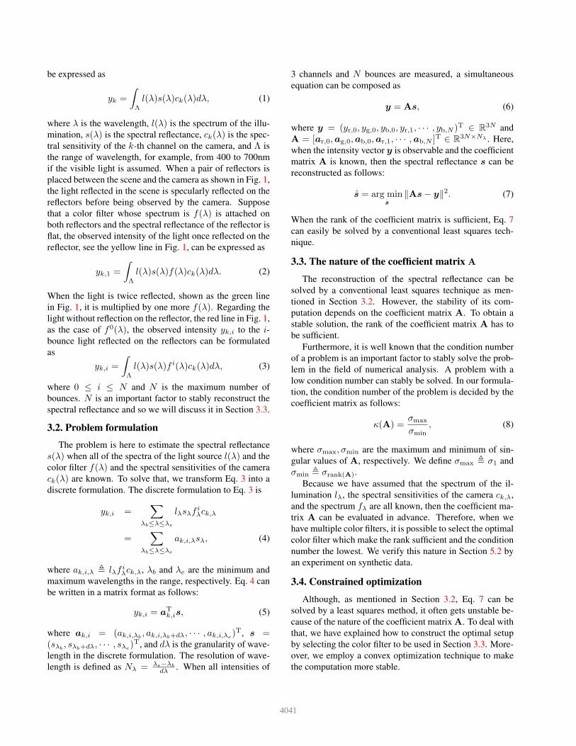
��
�Figure 2: The setup of a coupled mirror.
The spectral reflectance physically can neither be a neg-
ative value nor over 1.0. This fact can be used as a strong
box constraint. We can adopt a smoothness constraint on
the spectral reflectance since it is often measured in the real
world. Thus, we can rewrite Eq. 7 as
s = arg mins
{
‖As− y‖2 + α∫
Λ
(
∂2s(λ)∂λ2
)2
dλ
}
,
s.t. 0 ≤ s(λ) ≤ 1 (λ ∈ Λ), (9)
where α is the coefficient for the smoothness term. Then,
Eq. 9 can be expressed in a matrix format as
s = arg mins
{
‖As− y‖2 + α‖Ds‖2}
,
s.t. 0 ≤ sλ ≤ 1 (λb ≤ λ ≤ λe), (10)
where D is the second-order difference matrix. The ob-
jective function in Eq. 10 can be expressed in a quadratic
program format as
‖As− y‖2 + α‖Ds‖2
= sT(AT
A+ αDTD)s− 2yT
As+ yTy.(11)
Since the third term yTy is constant, then Eq. 10 is equiva-
lent to
s = arg mins
{
sT(AT
A+ αDTD)s− 2yT
As}
,
s.t. 0 ≤ sλ ≤ 1 (λb ≤ λ ≤ λe). (12)
We solve Eq. 12 by using the quadratic cone programming
technique [6]. To implement that optimization program, we
utilize the python optimization library cvxopt [1].
4. Various setups as implementation
In Section 3, we have explained our technique of one-
shot hyperspectral imaging by using faced mirrors. In order
to implement the technique, various setups are available. In
this section, we introduce two types of feasible setups by
using a coupled mirror and a kaleidoscope.
4.1. Coupled mirror geometry
The simplest setup uses a pair of planar reflectors, faced
to each other, on which color filters are attached. This setup
is generally called a coupled mirror. First, we assume that
the same filters are attached on both reflectors. Figure 2 il-
lustrates the setup of a coupled mirror whose length is z and
rrrrrr ����
rrrrrr ���������� ��� ��� ��� ��� ���
������ ��� ��� ��� ��� ���
������ ��� ��� ��� ��� ���
������ ��� ��� ��� ��� ���
������ ��� ��� ��� ��� ���
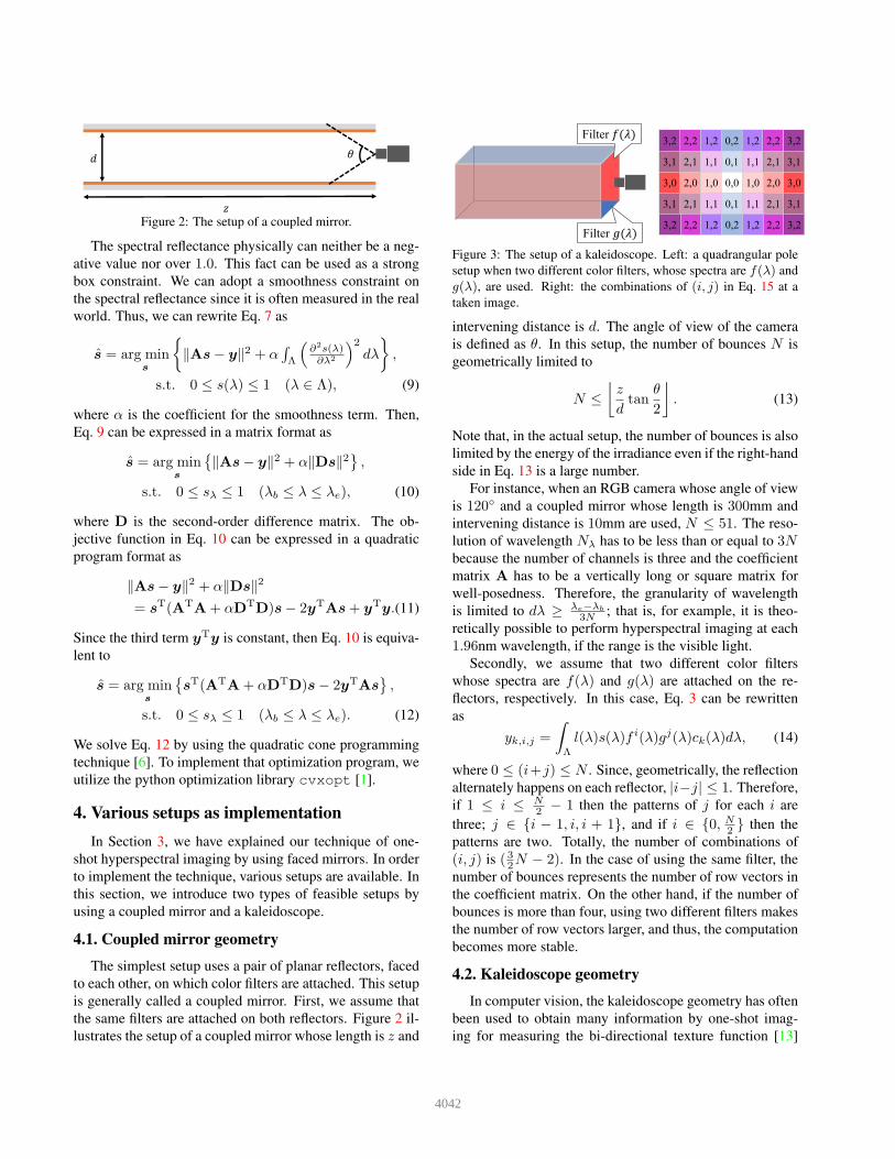
Figure 3: The setup of a kaleidoscope. Left: a quadrangular pole
setup when two different color filters, whose spectra are f(λ) and
g(λ), are used. Right: the combinations of (i, j) in Eq. 15 at a
taken image.
intervening distance is d. The angle of view of the camera
is defined as θ. In this setup, the number of bounces N is
geometrically limited to
N ≤
⌊
z
dtan
θ
2
⌋
. (13)
Note that, in the actual setup, the number of bounces is also
limited by the energy of the irradiance even if the right-hand
side in Eq. 13 is a large number.
For instance, when an RGB camera whose angle of view
is 120◦ and a coupled mirror whose length is 300mm and
intervening distance is 10mm are used, N ≤ 51. The reso-
lution of wavelength Nλ has to be less than or equal to 3Nbecause the number of channels is three and the coefficient
matrix A has to be a vertically long or square matrix for
well-posedness. Therefore, the granularity of wavelength
is limited to dλ ≥ λe−λb
3N ; that is, for example, it is theo-
retically possible to perform hyperspectral imaging at each
1.96nm wavelength, if the range is the visible light.
Secondly, we assume that two different color filters
whose spectra are f(λ) and g(λ) are attached on the re-
flectors, respectively. In this case, Eq. 3 can be rewritten
as
yk,i,j =
∫
Λ
l(λ)s(λ)f i(λ)gj(λ)ck(λ)dλ, (14)
where 0 ≤ (i+j) ≤ N . Since, geometrically, the reflection
alternately happens on each reflector, |i−j| ≤ 1. Therefore,
if 1 ≤ i ≤ N2 − 1 then the patterns of j for each i are
three; j ∈ {i − 1, i, i + 1}, and if i ∈ {0, N2 } then the
patterns are two. Totally, the number of combinations of
(i, j) is ( 32N − 2). In the case of using the same filter, the
number of bounces represents the number of row vectors in
the coefficient matrix. On the other hand, if the number of
bounces is more than four, using two different filters makes
the number of row vectors larger, and thus, the computation
becomes more stable.
4.2. Kaleidoscope geometry
In computer vision, the kaleidoscope geometry has often
been used to obtain many information by one-shot imag-
ing for measuring the bi-directional texture function [13]
4042
400 450 500 550 600 650 700
Wavelength[nm]
0.0
0.2
0.4
0.6
0.8
1.0 R sensitivity
G sensitivity
B sensitivity
#43 Deep Pink
#88 Light Green
#67 Light SkyBlue
Orange filterfor experiment
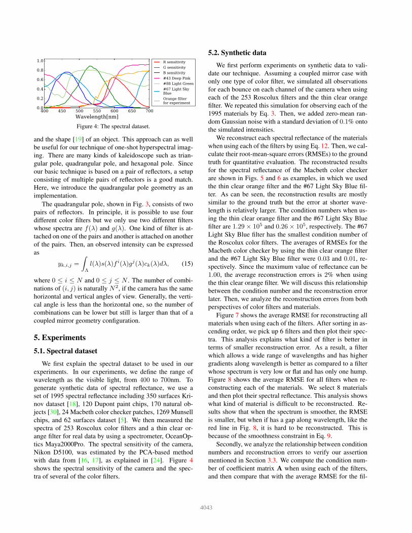
Figure 4: The spectral dataset.
and the shape [19] of an object. This approach can as well
be useful for our technique of one-shot hyperspectral imag-
ing. There are many kinds of kaleidoscope such as trian-
gular pole, quadrangular pole, and hexagonal pole. Since
our basic technique is based on a pair of reflectors, a setup
consisting of multiple pairs of reflectors is a good match.
Here, we introduce the quadrangular pole geometry as an
implementation.
The quadrangular pole, shown in Fig. 3, consists of two
pairs of reflectors. In principle, it is possible to use four
different color filters but we only use two different filters
whose spectra are f(λ) and g(λ). One kind of filter is at-
tached on one of the pairs and another is attached on another
of the pairs. Then, an observed intensity can be expressed
as
yk,i,j =
∫
Λ
l(λ)s(λ)f i(λ)gj(λ)ck(λ)dλ, (15)
where 0 ≤ i ≤ N and 0 ≤ j ≤ N . The number of combi-
nations of (i, j) is naturally N2, if the camera has the same
horizontal and vertical angles of view. Generally, the verti-
cal angle is less than the horizontal one, so the number of
combinations can be lower but still is larger than that of a
coupled mirror geometry configuration.
5. Experiments
5.1. Spectral dataset
We first explain the spectral dataset to be used in our
experiments. In our experiments, we define the range of
wavelength as the visible light, from 400 to 700nm. To
generate synthetic data of spectral reflectance, we use a
set of 1995 spectral reflectance including 350 surfaces Kri-
nov dataset [18], 120 Dupont paint chips, 170 natural ob-
jects [30], 24 Macbeth color checker patches, 1269 Munsell
chips, and 62 surfaces dataset [5]. We then measured the
spectra of 253 Roscolux color filters and a thin clear or-
ange filter for real data by using a spectrometer, OceanOp-
tics Maya2000Pro. The spectral sensitivity of the camera,
Nikon D5100, was estimated by the PCA-based method
with data from [16, 17], as explained in [24]. Figure 4
shows the spectral sensitivity of the camera and the spec-
tra of several of the color filters.
5.2. Synthetic data
We first perform experiments on synthetic data to vali-
date our technique. Assuming a coupled mirror case with
only one type of color filter, we simulated all observations
for each bounce on each channel of the camera when using
each of the 253 Roscolux filters and the thin clear orange
filter. We repeated this simulation for observing each of the
1995 materials by Eq. 3. Then, we added zero-mean ran-
dom Gaussian noise with a standard deviation of 0.1% onto
the simulated intensities.
We reconstruct each spectral reflectance of the materials
when using each of the filters by using Eq. 12. Then, we cal-
culate their root-mean-square errors (RMSEs) to the ground
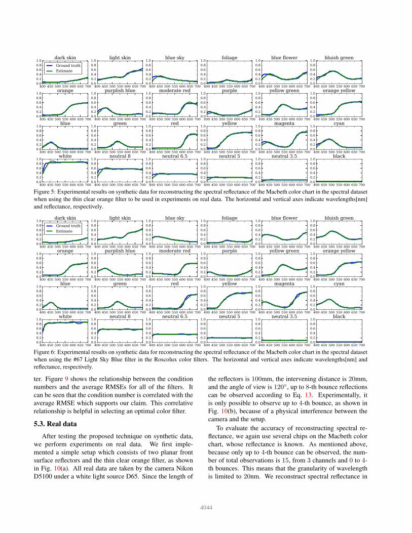
truth for quantitative evaluation. The reconstructed results
for the spectral reflectance of the Macbeth color checker
are shown in Figs. 5 and 6 as examples, in which we used
the thin clear orange filter and the #67 Light Sky Blue fil-
ter. As can be seen, the reconstruction results are mostly
similar to the ground truth but the error at shorter wave-
length is relatively larger. The condition numbers when us-
ing the thin clear orange filter and the #67 Light Sky Blue
filter are 1.29× 10⁵ and 0.26× 10⁵, respectively. The #67
Light Sky Blue filter has the smallest condition number of
the Roscolux color filters. The averages of RMSEs for the
Macbeth color checker by using the thin clear orange filter
and the #67 Light Sky Blue filter were 0.03 and 0.01, re-
spectively. Since the maximum value of reflectance can be
1.00, the average reconstruction errors is 2% when using
the thin clear orange filter. We will discuss this relationship
between the condition number and the reconstruction error
later. Then, we analyze the reconstruction errors from both
perspectives of color filters and materials.
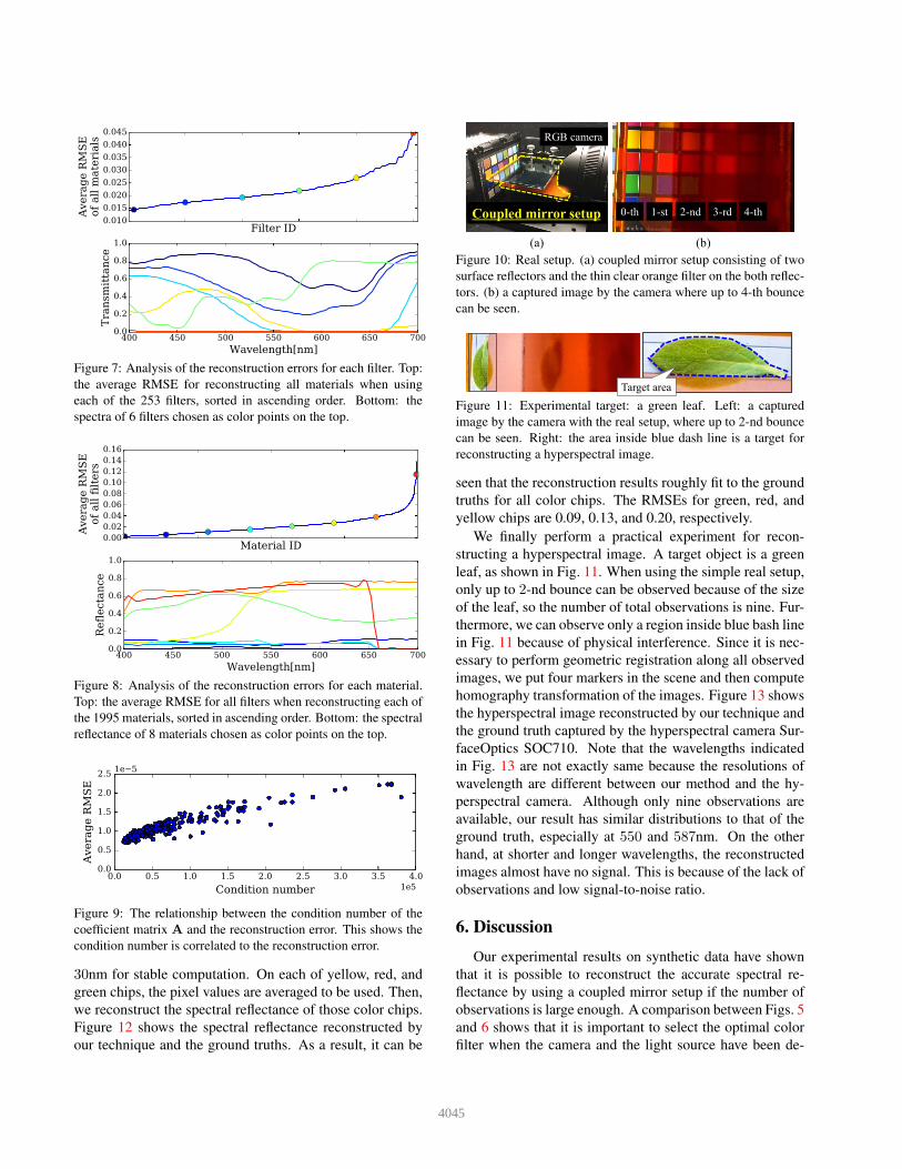
Figure 7 shows the average RMSE for reconstructing all
materials when using each of the filters. After sorting in as-
cending order, we pick up 6 filters and then plot their spec-
tra. This analysis explains what kind of filter is better in
terms of smaller reconstruction error. As a result, a filter
which allows a wide range of wavelengths and has higher
gradients along wavelength is better as compared to a filter
whose spectrum is very low or flat and has only one hump.
Figure 8 shows the average RMSE for all filters when re-
constructing each of the materials. We select 8 materials
and then plot their spectral reflectance. This analysis shows
what kind of material is difficult to be reconstructed. Re-
sults show that when the spectrum is smoother, the RMSE
is smaller, but when if has a gap along wavelength, like the
red line in Fig. 8, it is hard to be reconstructed. This is
because of the smoothness constraint in Eq. 9.
Secondly, we analyze the relationship between condition
numbers and reconstruction errors to verify our assertion
mentioned in Section 3.3. We compute the condition num-
ber of coefficient matrix A when using each of the filters,
and then compare that with the average RMSE for the fil-
4043
400 450 500 550 600 650 7000.00.20.40.60.81.0
dark skin
Ground truth
Estimate
400 450 500 550 600 650 7000.00.20.40.60.81.0
light skin
400 450 500 550 600 650 7000.00.20.40.60.81.0
blue sky
400 450 500 550 600 650 7000.00.20.40.60.81.0
foliage
400 450 500 550 600 650 7000.00.20.40.60.81.0
blue flower
400 450 500 550 600 650 7000.00.20.40.60.81.0
bluish green
400 450 500 550 600 650 7000.00.20.40.60.81.0
orange
400 450 500 550 600 650 7000.00.20.40.60.81.0
purplish blue
400 450 500 550 600 650 7000.00.20.40.60.81.0
moderate red
400 450 500 550 600 650 7000.00.20.40.60.81.0
purple
400 450 500 550 600 650 7000.00.20.40.60.81.0
yellow green
400 450 500 550 600 650 7000.00.20.40.60.81.0
orange yellow
400 450 500 550 600 650 7000.00.20.40.60.81.0
blue
400 450 500 550 600 650 7000.00.20.40.60.81.0
green
400 450 500 550 600 650 7000.00.20.40.60.81.0
red
400 450 500 550 600 650 7000.00.20.40.60.81.0
yellow
400 450 500 550 600 650 7000.00.20.40.60.81.0
magenta
400 450 500 550 600 650 7000.00.20.40.60.81.0
cyan
400 450 500 550 600 650 7000.00.20.40.60.81.0
white
400 450 500 550 600 650 7000.00.20.40.60.81.0
neutral 8
400 450 500 550 600 650 7000.00.20.40.60.81.0
neutral 6.5
400 450 500 550 600 650 7000.00.20.40.60.81.0
neutral 5
400 450 500 550 600 650 7000.00.20.40.60.81.0
neutral 3.5
400 450 500 550 600 650 7000.00.20.40.60.81.0
black
Figure 5: Experimental results on synthetic data for reconstructing the spectral reflectance of the Macbeth color chart in the spectral dataset
when using the thin clear orange filter to be used in experiments on real data. The horizontal and vertical axes indicate wavelengths[nm]
and reflectance, respectively.
400 450 500 550 600 650 7000.00.20.40.60.81.0
dark skin
Ground truth
Estimate
400 450 500 550 600 650 7000.00.20.40.60.81.0
light skin
400 450 500 550 600 650 7000.00.20.40.60.81.0
blue sky
400 450 500 550 600 650 7000.00.20.40.60.81.0
foliage
400 450 500 550 600 650 7000.00.20.40.60.81.0
blue flower
400 450 500 550 600 650 7000.00.20.40.60.81.0
bluish green
400 450 500 550 600 650 7000.00.20.40.60.81.0
orange
400 450 500 550 600 650 7000.00.20.40.60.81.0
purplish blue
400 450 500 550 600 650 7000.00.20.40.60.81.0
moderate red
400 450 500 550 600 650 7000.00.20.40.60.81.0
purple
400 450 500 550 600 650 7000.00.20.40.60.81.0
yellow green
400 450 500 550 600 650 7000.00.20.40.60.81.0
orange yellow
400 450 500 550 600 650 7000.00.20.40.60.81.0
blue
400 450 500 550 600 650 7000.00.20.40.60.81.0
green
400 450 500 550 600 650 7000.00.20.40.60.81.0
red
400 450 500 550 600 650 7000.00.20.40.60.81.0
yellow
400 450 500 550 600 650 7000.00.20.40.60.81.0
magenta
400 450 500 550 600 650 7000.00.20.40.60.81.0
cyan
400 450 500 550 600 650 7000.00.20.40.60.81.0
white
400 450 500 550 600 650 7000.00.20.40.60.81.0
neutral 8
400 450 500 550 600 650 7000.00.20.40.60.81.0
neutral 6.5
400 450 500 550 600 650 7000.00.20.40.60.81.0
neutral 5
400 450 500 550 600 650 7000.00.20.40.60.81.0
neutral 3.5
400 450 500 550 600 650 7000.00.20.40.60.81.0
black
Figure 6: Experimental results on synthetic data for reconstructing the spectral reflectance of the Macbeth color chart in the spectral dataset
when using the #67 Light Sky Blue filter in the Roscolux color filters. The horizontal and vertical axes indicate wavelengths[nm] and
reflectance, respectively.
ter. Figure 9 shows the relationship between the condition
numbers and the average RMSEs for all of the filters. It
can be seen that the condition number is correlated with the
average RMSE which supports our claim. This correlative
relationship is helpful in selecting an optimal color filter.
5.3. Real data
After testing the proposed technique on synthetic data,
we perform experiments on real data. We first imple-
mented a simple setup which consists of two planar front
surface reflectors and the thin clear orange filter, as shown
in Fig. 10(a). All real data are taken by the camera Nikon
D5100 under a white light source D65. Since the length of
the reflectors is 100mm, the intervening distance is 20mm,
and the angle of view is 120◦, up to 8-th bounce reflections
can be observed according to Eq. 13. Experimentally, it
is only possible to observe up to 4-th bounce, as shown in
Fig. 10(b), because of a physical interference between the
camera and the setup.
To evaluate the accuracy of reconstructing spectral re-
flectance, we again use several chips on the Macbeth color
chart, whose reflectance is known. As mentioned above,
because only up to 4-th bounce can be observed, the num-
ber of total observations is 15, from 3 channels and 0 to 4-
th bounces. This means that the granularity of wavelength
is limited to 20nm. We reconstruct spectral reflectance in
4044
Filter ID0.010
0.015
0.020
0.025
0.030
0.035
0.040
0.045
Ave
rag
e R
MS
Eof
all
mate
rials
400 450 500 550 600 650 700
Wavelength[nm]
0.0
0.2
0.4
0.6
0.8
1.0
Tra
nsm
itta
nce
Figure 7: Analysis of the reconstruction errors for each filter. Top:
the average RMSE for reconstructing all materials when using
each of the 253 filters, sorted in ascending order. Bottom: the
spectra of 6 filters chosen as color points on the top.
Material ID0.000.020.040.060.080.100.120.140.16
Ave
rag
e R
MS
Eof
all
fil
ters
400 450 500 550 600 650 700
Wavelength[nm]
0.0
0.2
0.4
0.6
0.8
1.0
Refl
ect
an
ce
Figure 8: Analysis of the reconstruction errors for each material.
Top: the average RMSE for all filters when reconstructing each of
the 1995 materials, sorted in ascending order. Bottom: the spectral
reflectance of 8 materials chosen as color points on the top.
0.0 0.5 1.0 1.5 2.0 2.5 3.0 3.5 4.0
Condition number 1e5
0.0
0.5
1.0
1.5
2.0
2.5
Ave
rag
e R
MS
E
1e 5
Figure 9: The relationship between the condition number of the
coefficient matrix A and the reconstruction error. This shows the
condition number is correlated to the reconstruction error.
30nm for stable computation. On each of yellow, red, and
green chips, the pixel values are averaged to be used. Then,
we reconstruct the spectral reflectance of those color chips.
Figure 12 shows the spectral reflectance reconstructed by
our technique and the ground truths. As a result, it can be
(a) (b)
RGB camera
Coupled mirror setup 1-st 2-nd 3-rd0-th 4-th
Figure 10: Real setup. (a) coupled mirror setup consisting of two
surface reflectors and the thin clear orange filter on the both reflec-
tors. (b) a captured image by the camera where up to 4-th bounce
can be seen.
Target area
Figure 11: Experimental target: a green leaf. Left: a captured
image by the camera with the real setup, where up to 2-nd bounce
can be seen. Right: the area inside blue dash line is a target for
reconstructing a hyperspectral image.
seen that the reconstruction results roughly fit to the ground
truths for all color chips. The RMSEs for green, red, and
yellow chips are 0.09, 0.13, and 0.20, respectively.
We finally perform a practical experiment for recon-
structing a hyperspectral image. A target object is a green
leaf, as shown in Fig. 11. When using the simple real setup,
only up to 2-nd bounce can be observed because of the size
of the leaf, so the number of total observations is nine. Fur-
thermore, we can observe only a region inside blue bash line
in Fig. 11 because of physical interference. Since it is nec-
essary to perform geometric registration along all observed
images, we put four markers in the scene and then compute
homography transformation of the images. Figure 13 shows
the hyperspectral image reconstructed by our technique and
the ground truth captured by the hyperspectral camera Sur-
faceOptics SOC710. Note that the wavelengths indicated
in Fig. 13 are not exactly same because the resolutions of
wavelength are different between our method and the hy-
perspectral camera. Although only nine observations are
available, our result has similar distributions to that of the
ground truth, especially at 550 and 587nm. On the other
hand, at shorter and longer wavelengths, the reconstructed
images almost have no signal. This is because of the lack of
observations and low signal-to-noise ratio.
6. Discussion
Our experimental results on synthetic data have shown
that it is possible to reconstruct the accurate spectral re-
flectance by using a coupled mirror setup if the number of
observations is large enough. A comparison between Figs. 5
and 6 shows that it is important to select the optimal color
filter when the camera and the light source have been de-
4045
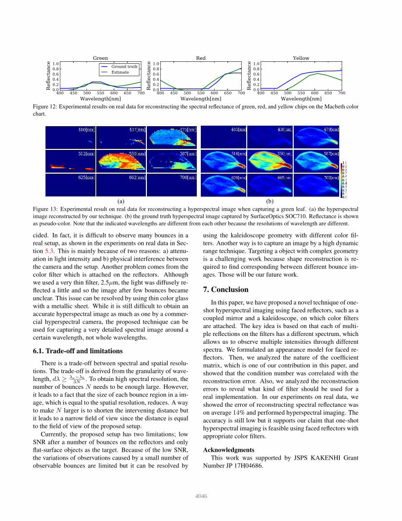
400 450 500 550 600 650 700
Wavelength[nm]
0.00.20.40.60.81.0
Refl
ect
an
ce
Green
Ground truth
Estimate
400 450 500 550 600 650 700
Wavelength[nm]
0.00.20.40.60.81.0
Refl
ect
an
ce
Red
400 450 500 550 600 650 700
Wavelength[nm]
0.00.20.40.60.81.0
Refl
ect
an
ce
Yellow
Figure 12: Experimental results on real data for reconstructing the spectral reflectance of green, red, and yellow chips on the Macbeth color
chart.
(a) (b)
Figure 13: Experimental result on real data for reconstructing a hyperspectral image when capturing a green leaf. (a) the hyperspectral
image reconstructed by our technique. (b) the ground truth hyperspectral image captured by SurfaceOptics SOC710. Reflectance is shown
as pseudo-color. Note that the indicated wavelengths are different from each other because the resolutions of wavelength are different.
cided. In fact, it is difficult to observe many bounces in a
real setup, as shown in the experiments on real data in Sec-
tion 5.3. This is mainly because of two reasons: a) attenu-
ation in light intensity and b) physical interference between
the camera and the setup. Another problem comes from the
color filter which is attached on the reflectors. Although
we used a very thin filter, 2.5µm, the light was diffusely re-
flected a little and so the image after few bounces became
unclear. This issue can be resolved by using thin color glass
with a metallic sheet. While it is still difficult to obtain an
accurate hyperspectral image as much as one by a commer-
cial hyperspectral camera, the proposed technique can be
used for capturing a very detailed spectral image around a
certain wavelength, not whole wavelengths.
6.1. Tradeoff and limitations
There is a trade-off between spectral and spatial resolu-
tions. The trade-off is derived from the granularity of wave-
length, dλ ≥ λe−λb
3N . To obtain high spectral resolution, the
number of bounces N needs to be enough large. However,
it leads to a fact that the size of each bounce region in a im-
age, which is equal to the spatial resolution, reduces. A way
to make N larger is to shorten the intervening distance but
it leads to a narrow field of view since the distance is equal
to the field of view of the proposed setup.
Currently, the proposed setup has two limitations; low
SNR after a number of bounces on the reflectors and only
flat-surface objects as the target. Because of the low SNR,
the variations of observations caused by a small number of
observable bounces are limited but it can be resolved by
using the kaleidoscope geometry with different color fil-
ters. Another way is to capture an image by a high dynamic
range technique. Targeting a object with complex geometry
is a challenging work because shape reconstruction is re-
quired to find corresponding between different bounce im-
ages. Those will be our future work.
7. Conclusion
In this paper, we have proposed a novel technique of one-
shot hyperspectral imaging using faced reflectors, such as a
coupled mirror and a kaleidoscope, on which color filters
are attached. The key idea is based on that each of multi-
ple reflections on the filters has a different spectrum, which
allows us to observe multiple intensities through different
spectra. We formulated an appearance model for faced re-
flectors. Then, we analyzed the nature of the coefficient
matrix, which is one of our contribution in this paper, and
showed that the condition number was correlated with the
reconstruction error. Also, we analyzed the reconstruction
errors to reveal what kind of filter should be used for a
real implementation. In our experiments on real data, we
showed the error of reconstructing spectral reflectance was
on average 14% and performed hyperspectral imaging. The
accuracy is still low but it supports our claim that one-shot
hyperspectral imaging is feasible using faced reflectors with
appropriate color filters.
Acknowledgments
This work was supported by JSPS KAKENHI Grant
Number JP 17H04686.
4046

References
[1] Cvxopt: Python software for convex optimization. http:
//cvxopt.org/. Accessed: 2016-11-12. 4
[2] F. M. Abed, S. H. Amirshahi, and M. R. M. Abed. Recon-
struction of reflectance data using an interpolation technique.
Journal of the Optical Society of America A, 26(3):613–624,
2009. 2
[3] A. Abrardo, L. Alparone, I. Cappellini, and A. Prosperi.
Color constancy from multispectral images. In Proc. of Inter-
national Conference on Image Processing (ICIP), volume 3,
pages 570–574. IEEE, 1999. 1
[4] G. R. Arce, D. J. Brady, L. Carin, H. Arguello, and D. S.
Kittle. Compressive coded aperture spectral imaging: An
introduction. IEEE Signal Processing Magazine, 31(1):105–
115, 2014. 2
[5] K. Barnard, L. Martin, B. Funt, and A. Coath. A data
set for colour research. Color Research and Application,
27(3):147–151, 2002. 5
[6] S. Boyd and L. Vandenberghe, editors. Convex Optimization.
Cambridge University Press, 2004. 4
[7] C. Chi, H. Yoo, and M. Ben-Ezra. Multi-spectral imaging by
optimized wide band illumination. International Journal of
Computer Vision, 86(2-3):140–151, 2010. 2
[8] H. Du, X. Tong, X. Cao, and S. Lin. A prism-based sys-
tem for multispectral video acquisition. In Proc. of Interna-
tional Conference on Computer Vision (ICCV), pages 175–
182. IEEE, 2009. 2
[9] M. D’Zmura. Color constancy: surface color from changing
illumination. Journal of the Optical Society of America A,
9(3):490–493, 1992. 2
[10] K. Forbes, F. Nicolls, G. De Jager, and A. Voigt. Shape-from-
silhouette with two mirrors and an uncalibrated camera. In
Proc. of European Conference on Computer Vision (ECCV),
pages 165–178. Springer, 2006. 2
[11] N. Gat. Imaging spectroscopy using tunable filters: a review.
In Proc. SPIE Wavelet Applications VII, pages 50–64, 2000.
2
[12] R. Habel, M. Kudenov, and M. Wimmer. Practical spectral
photography. In Computer graphics forum, volume 31, pages
449–458. Wiley Online Library, 2012. 2
[13] J. Y. Han and K. Perlin. Measuring bidirectional texture
reflectance with a kaleidoscope. ACM Trans. on Graph.,
22(3):741–748, 2003. 2, 4
[14] S. Han, I. Sato, T. Okabe, and Y. Sato. Fast spectral re-
flectance recovery using dlp projector. International Journal
of Computer Vision, 110(2):172–184, 2014. 2
[15] M. Hinnrichs and M. A. Massie. New approach to imaging
spectroscopy using diffractive optics, 1997. 2
[16] J. Jiang, D. Liu, J. Gu, and S. Susstrunk. What is the
space of spectral sensitivity functions for digital color cam-
eras? In IEEE Workshop on Applications of Computer Vision
(WACV), pages 168–179. IEEE, 2013. 5
[17] R. Kawakami, Y. Matsushita, J. Wright, M. Ben-Ezra, Y.-
W. Tai, and K. Ikeuchi. High-resolution hyperspectral imag-
ing via matrix factorization. In Proc. of IEEE Conference
on Computer Vision and Pattern Recognition (CVPR), pages
2329–2336. IEEE, 2011. 5
[18] E. L. Krinov. Spectral reflectance properties of natural for-
mations. Technical report, National Research Council of
Canada, 1947. 5
[19] D. Lanman, D. Crispell, and G. Taubin. Surround structured
lighting for full object scanning. In Proc. International Con-
ference on 3-D Digital Imaging and Modeling, pages 107–
116. IEEE, 2007. 5
[20] A. Manakov, J. Restrepo, O. Klehm, R. Hegedus, E. Eise-
mann, H.-P. Seidel, and I. Ihrke. A reconfigurable camera
add-on for high dynamic range, multispectral, polarization,
and light-field imaging. ACM Trans. on Graph., 32(4):47–1,
2013. 2
[21] P. J. Miller and C. C. Hoyt. Multispectral imaging with a
liquid crystal tunable filter. In Photonics for Industrial Ap-
plications, pages 354–365. International Society for Optics
and Photonics, 1995. 2
[22] P. Morovic and G. D. Finlayson. Metamer-set-based ap-
proach to estimating surface reflectance from camera rgb.
Journal of the Optical Society of America A, 23(8):1814–
1822, 2006. 2
[23] R. M. Nguyen, D. K. Prasad, and M. S. Brown. Training-
based spectral reconstruction from a single rgb image. In
Proc. of European Conference on Computer Vision (ECCV),
pages 186–201. Springer, 2014. 2
[24] S. W. Oh, M. S. Brown, M. Pollefeys, and S. J. Kim. Do
it yourself hyperspectral imaging with everyday digital cam-
eras. In Proc. of IEEE Conference on Computer Vision and
Pattern Recognition (CVPR), pages 2461–2469, 2016. 2, 5
[25] J.-I. Park, M.-H. Lee, M. D. Grossberg, and S. K. Na-
yar. Multispectral imaging using multiplexed illumination.
In Proc. of International Conference on Computer Vision
(ICCV), pages 1–8. IEEE, 2007. 2
[26] I. Reshetouski, A. Manakov, H.-P. Seidel, and I. Ihrke.
Three-dimensional kaleidoscopic imaging. In Proc. of IEEE
Conference on Computer Vision and Pattern Recognition
(CVPR), pages 353–360. IEEE, 2011. 2
[27] D. W. Stein, S. G. Beaven, L. E. Hoff, E. M. Winter, A. P.
Schaum, and A. D. Stocker. Anomaly detection from hy-
perspectral imagery. IEEE Signal Processing Magazine,
19(1):58–69, 2002. 1
[28] S. Tominaga. Multichannel vision system for estimating sur-
face and illumination functions. Journal of the Optical Soci-
ety of America A, 13(11):2163–2173, 1996. 2
[29] S. Tominaga and R. Okajima. Object recognition by multi-
spectral imaging with a liquid crystal filter. In Proc. of In-
ternational Conference on Pattern Recognition (ICPR), vol-
ume 1, pages 708–711. IEEE, 2000. 1
[30] M. J. Vrhel, R. Gershon, and L. S. Iwan. Measurement and
analysis of object reflectance spectra. Color Research and
Application, 19(1):4–9, 1994. 5
4047