HAL Id: hal-01674562https://hal.archives-ouvertes.fr/hal-01674562

Submitted on 3 Jan 2018

HAL is a multi-disciplinary open accessarchive for the deposit and dissemination of sci-entific research documents, whether they are pub-lished or not. The documents may come fromteaching and research institutions in France orabroad, or from public or private research centers.

L’archive ouverte pluridisciplinaire HAL, estdestinée au dépôt et à la diffusion de documentsscientifiques de niveau recherche, publiés ou non,émanant des établissements d’enseignement et derecherche français ou étrangers, des laboratoirespublics ou privés.

On the validation of integrated DIC with tapered doublecantilever beam tests

Thiago Melo Grabois, Jan Neggers, Laurent Ponson, François Hild, RomildoDias Toledo Filho

To cite this version:Thiago Melo Grabois, Jan Neggers, Laurent Ponson, François Hild, Romildo Dias Toledo Filho. Onthe validation of integrated DIC with tapered double cantilever beam tests. Engineering FractureMechanics, Elsevier, 2018, 191, pp.311-323. �10.1016/j.engfracmech.2017.12.015�. �hal-01674562�

On the validation of integrated DIC with

tapered double cantilever beam tests

Thiago Melo Graboisa,c,∗, Jan Neggersb, Laurent Ponsonc, Francois Hildb,and Romildo Dias Toledo Filhoa

aLaboratory of Structures and Materials Professor Lobo Carneiro (LabEST), COPPE /UFRJ, P.O. Box 68506, Zip code 21941-972, Rio de Janeiro, Brazil

bLaboratoire de Mecanique et Technologie (LMT), ENS Paris-Saclay / CNRS /University Paris-Saclay, 61 Avenue du President Wilson, 94235 Cachan Cedex, France

cInstitut Jean le Rond d’Alembert, UPMC - CNRS, Sorbonne Universites4 Place Jussieu, 75005 Paris, France

Abstract

Full-field measurement methods such as integrated digital image correla-

tion bypass the need for post-processing the displacement data upon mini-

mizing the gap between simulation and experiment. This paper discusses the

validation of this method by comparing its results with an approach based

on compliance values measured from crack mouth opening displacement and

load data to calculate mode I stress intensity factors (SIFs) and crack tip po-

sitions. Tapered double cantilever beams are used as a test case to evaluate

the quasi-brittle fracture response of PMMA. The results demonstrate the

ability of the proposed technique to obtain accurate determinations of SIFs

and crack length using the tapered geometry. Additionally, both methods

yield consistent results, which validates the integrated approach against an

independent method.

∗corresponding authorEmail address: thiagomgrabois@coc.ufrj.br (Thiago Melo Grabois)

Preprint submitted to Engineering Fracture Mechanics December 11, 2017

Keywords: Compliance method, Digital image correlation, Stress intensity

factor measurement, Stable crack propagation

1. Introduction

Accurately measuring the material toughness is a difficult task for sev-

eral reasons. First, the toughness is defined as the critical driving force (or

critical elastic energy release rate) at which a crack propagates. In principle,

this means that both the crack tip position and the total energy released5

during crack advance must be tracked during the test, thereby rendering

the measurement very indirect and prone to multiple causes of experimen-

tal errors. Second, the local toughness value, namely KIc may depend on

the crack growth velocity v. These facts require the development of fracture

tests where the crack propagation speed can be controlled and tuned over10

a broad range. Furthermore, measuring toughness requires stable fracture,

both from the point of view of crack propagation (i.e., the crack must stop

when the external driving force is stopped) and trajectory that must be rather

straight. This can be particularly challenging in brittle solids (e.g., ceramics

and glass). The choice of the geometry of the fracture test that controls the15

crack stability then becomes essential.

Different fracture tests have been proposed to handle these challenges.

Some of them, such as Single Edge Notch Bending (SENB) and Compact

Tension (CT) tests [1], present a short crack propagation length and a rather

poor stability of the fracture process [2]. Alternatively, the Tapered Double20

Cantilever Beam (TDCB) test enables for significant stability of the fracture

process in mode I [3], which is appealing for brittle materials. Further, it

2

allows for the exploration of a large range of crack growth velocities [4, 5].

Different TDCB specimens were used to perform mode I fracture tests of ad-

hesive bond joints [6, 7, 8] and, for instance, to study the R-curve behavior in25

quasi-brittle wood materials [9] taking advantage of the crack growth stabil-

ity provided by the tapered shape. In many displacement-controlled TDCB

experiments, it has been observed that the compliance increases linearly with

the crack length. Moreover, previous studies [8, 10, 11] supported this fact

using beam theory. As the energy release rate [6] depends on the derivative30

of the compliance, its value is then constant when the crack propagates.

Recently, the TDCB geometry was modified by significantly enlarging the

arms from which the displacement is prescribed during the test [4, 5]. This

new design results in an exponential decrease of the elastic energy release rate

with crack length; and thus in an improved stability of the fracture process,35

thereby rendering the TDCB fracture test amenable to the study of brittle

solids.

Standardized test methods for measuring fracture toughness usually con-

sider global measurements provided by load cells and clip gauges (e.g., see

Ref. [1]). An alternative route consists in utilizing full-field measurements.40

Digital Image Correlation (DIC) was successfully used to monitor cracks in

various materials [12, 13, 14, 15, 16]. To determine Stress Intensity Factors

(SIFs) and crack tip positions, the measured displacement fields are sub-

sequently post-processed via projections onto known solutions of fractured

elastic media [12]. In the case of brittle fracture, it is assumed that, apart45

from the immediate vicinity of the crack tip, the material behaves elastically.

In this specific case, Williams’ series [17] describe the stress and displacement

3

fields as functions of mechanical parameters for different fracture modes. A

least-squares fit enables the SIF to be evaluated [12, 13, 14] provided the

crack tip position is known [18]. Dehnavi et al. [19] showed that this method50

may provide more accurate results compared to photoelasticity when evalu-

ating SIFs.

The aim of the present paper is to validate Integrated DIC [18, 20]. In-

stead of first measuring displacement fields and then projecting them onto

Williams’ series, the two steps are integrated into a single analysis where the55

sought amplitudes (e.g., SIFs, crack tip positions) are a direct result of the

registration method. This approach bypasses the need for post-processing the

displacement data, thereby reducing errors in the re-projection process [16].

This is of particular importance in the present case since the displacements

are very small [21]. The crack tip location and SIFs will be compared with60

analyses based upon compliance measurements obtained independently from

crack mouth opening displacement (CMOD) and load data.

The paper is organized as follows. First the experimental configuration

and the studied material are introduced. The procedure employed to measure

the compliance variations during crack growth that will be used herein as a65

validation tool is presented. The integrated DIC framework is then summa-

rized in order to follow crack propagation and estimate SIFs. The procedure

is then applied to the pictures of two TDCB tests and the measurements are

compared with the results of the compliance technique discussed herein.

4

2. TDCB fracture tests70

Experiments on Tapered Double Cantilever Beam (TDCB) specimens

were carried out under uniaxial tension using a Shimadzu (model AG-Xplus)

universal testing machine (with ±10 kN load capacity). In this experimental

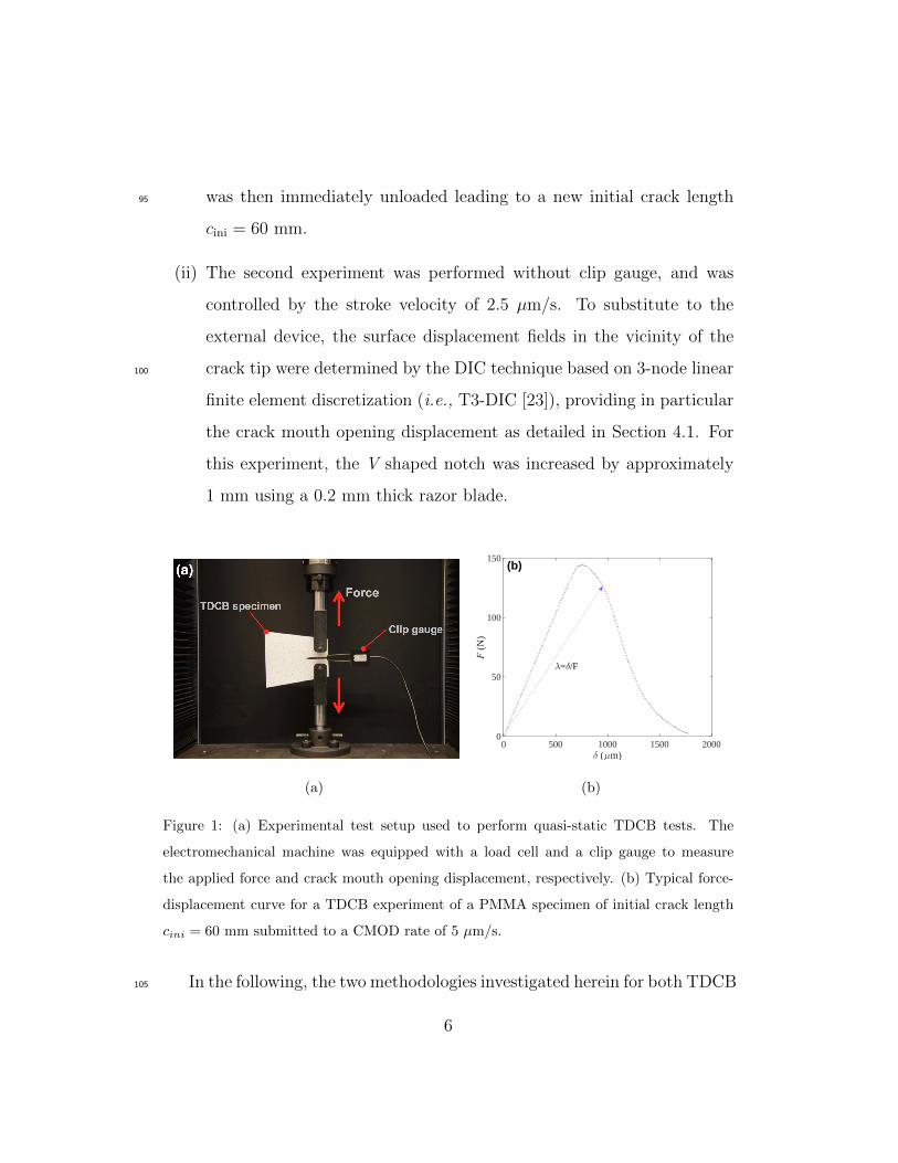
setup (see Figure 1(a)), a 1 kN load cell measured the force applied to the

specimen through the pins located in holes of diameter 2R = 5 mm. For the75

first experiment, a clip gauge was used to measure the crack mouth opening

displacement. Two steel grips were connected to the specimen by the pins

placed on both holes. The bottom one is fixed to the base and the top one,

which connects to the load sensor, is pushed up by the machine cross-head.

TDCB fracture tests were performed on a transparent thermoplastic,80

namely, poly-methyl methacrylate (PMMA), which is an archetype of brit-

tle amorphous material [22]. Two TDCB specimens were cast from a thin

PMMA sheet of 8 mm thickness using a laser cutting machine. The specimen

geometry is an isosceles trapezoid of shorter base h1 = 60 mm, longer base

h2 = 90 mm and height L = 100 mm, where a V shaped notch of 36.5 mm85

in length extends from the midpoint of h1. Although the main TDCB geom-

etry is the same for both experiments reported herein, they were managed

differently. Thus, the following procedures are discussed in this work:

(i) The first experiment was controlled by the crack mouth opening rate at

5 µm/s, i.e., with the clip gauge opening at constant velocity. In this90

case, the specimen V shaped notch experienced a straight elongation of

3.5 mm through laser cutting and an additional 20 mm crack extension

achieved by pre-loading the specimen under constant (i.e., 0.5 µm/s)

crack mouth opening velocity until the crack initiated. The sample

5

was then immediately unloaded leading to a new initial crack length95

cini = 60 mm.

(ii) The second experiment was performed without clip gauge, and was

controlled by the stroke velocity of 2.5 µm/s. To substitute to the

external device, the surface displacement fields in the vicinity of the

crack tip were determined by the DIC technique based on 3-node linear100

finite element discretization (i.e., T3-DIC [23]), providing in particular

the crack mouth opening displacement as detailed in Section 4.1. For

this experiment, the V shaped notch was increased by approximately

1 mm using a 0.2 mm thick razor blade.

(a)

δ (µm)0 500 1000 1500 2000

F (

N)

0

50

100

150(b)

λ=δ/F

(b)

Figure 1: (a) Experimental test setup used to perform quasi-static TDCB tests. The

electromechanical machine was equipped with a load cell and a clip gauge to measure

the applied force and crack mouth opening displacement, respectively. (b) Typical force-

displacement curve for a TDCB experiment of a PMMA specimen of initial crack length

cini = 60 mm submitted to a CMOD rate of 5 µm/s.

In the following, the two methodologies investigated herein for both TDCB105

6

fracture experiments are presented. First, a finite element (FE) based method

is employed to assess the elastic energy release rate and the crack speed from

the macroscopic mechanical behavior of the specimen, namely, the force-

crack opening response, an example of which is presented in Figure 1(b).

Then, it is shown that the TDCB geometry is amenable to a direct determi-110

nation of SIFs through DIC. This is an interesting alternative to the prior

methodology as it allows the fracture properties of the tested material to be

estimated without using load cells and CMOD gauges. In particular, such

alternative may be useful to measure toughnesses of high temperatures or for

high crack speeds for which mechanical gauges may be inefficient. Moreover,115

the DIC method provides the mode II stress intensity factor (in addition to

KI) that is of relevance for anisotropic solids as well as the amplitude of

non-singular terms such as the T-stress not accessible through the analysis

of the force-displacement response of the specimen.

3. Compliance method120

To implement this first method, only the force and crack opening dis-

placement data are considered. The goal is to determine the material frac-

ture toughness KIc and crack velocity v histories during the TDCB test.

The experimentally measured quantities are post-processed to determine the

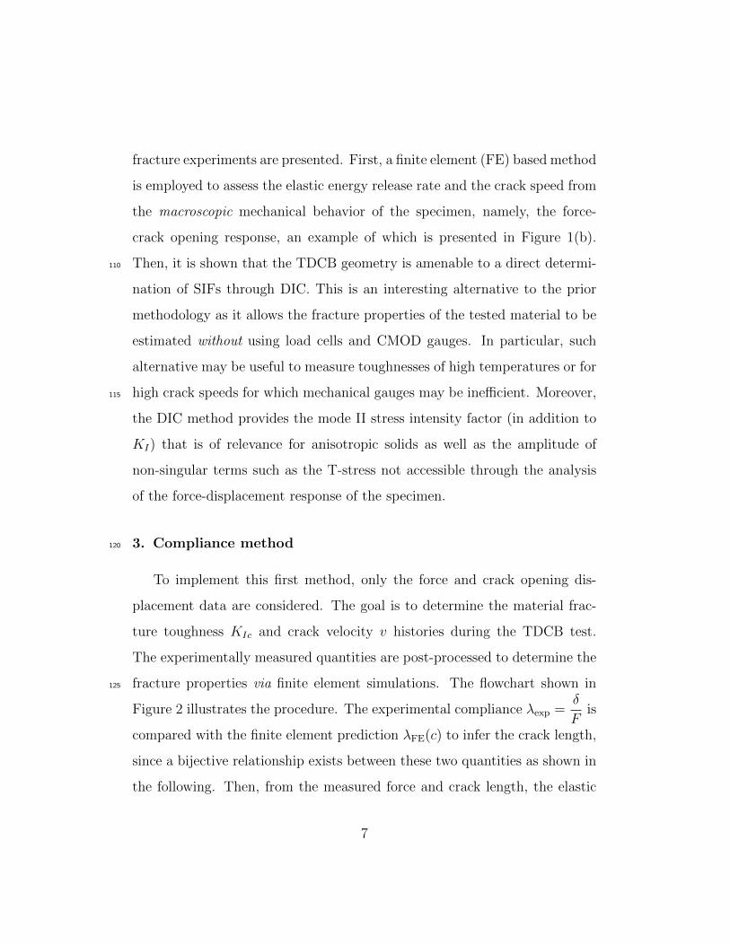
fracture properties via finite element simulations. The flowchart shown in125

Figure 2 illustrates the procedure. The experimental compliance λexp =δ

Fis

compared with the finite element prediction λFE(c) to infer the crack length,

since a bijective relationship exists between these two quantities as shown in

the following. Then, from the measured force and crack length, the elastic

7

energy release rate G = F 2gFE(c) follows. The crack velocity is computed as130

the time derivative of the crack positions. The objective of the finite element

simulations is thus to extract λFE(c) and gFE(c) that are geometry-dependent

functions.

This procedure is inspired from the compliance method used for instance

by Morel et al. [24] and was recently implemented with PMMA for the modi-135

fied TDCB geometry used in this work [4, 5]. The method is briefly described

in the sequel. It is based on the following two assumptions: i) brittle frac-

ture i.e., the material behaves elastically, except in a zone around the crack

tip, which is very small with respect to the sample size; ii) time-independent

behavior (e.g., viscosity is neglected). Numerical investigations of the me-140

chanical response of modified TDCB specimens are detailed in Refs. [4, 5].

8

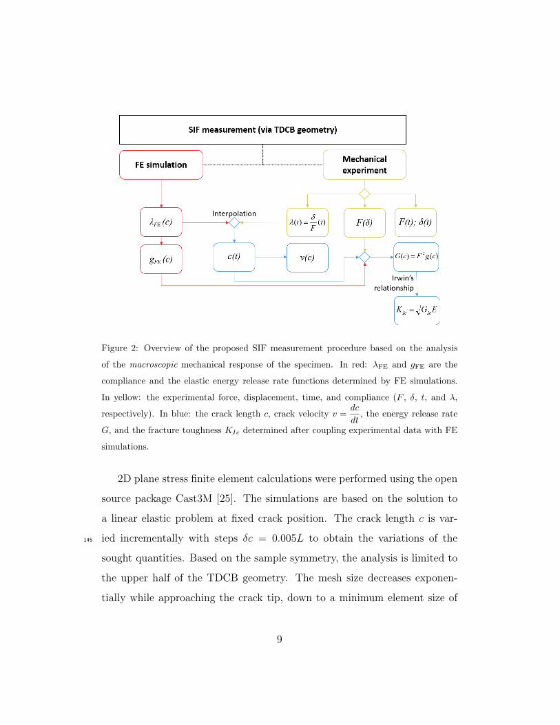
Figure 2: Overview of the proposed SIF measurement procedure based on the analysis

of the macroscopic mechanical response of the specimen. In red: λFE and gFE are the

compliance and the elastic energy release rate functions determined by FE simulations.

In yellow: the experimental force, displacement, time, and compliance (F , δ, t, and λ,

respectively). In blue: the crack length c, crack velocity v =dc

dt, the energy release rate

G, and the fracture toughness KIc determined after coupling experimental data with FE

simulations.

2D plane stress finite element calculations were performed using the open

source package Cast3M [25]. The simulations are based on the solution to

a linear elastic problem at fixed crack position. The crack length c is var-

ied incrementally with steps δc = 0.005L to obtain the variations of the145

sought quantities. Based on the sample symmetry, the analysis is limited to

the upper half of the TDCB geometry. The mesh size decreases exponen-

tially while approaching the crack tip, down to a minimum element size of

9

10−9L. For each crack tip position, the compliance is obtained by prescrib-

ing a unit force F0 and computing the corresponding displacement δ so that150

λFE = δ/F0. The elastic energy release rate is obtained from the variation of

mechanical energy for an incremental advance of the crack. The computed

value was confirmed through an independent method based on the so-called

compliance formula (see Equation (3)). The finite element solution for the

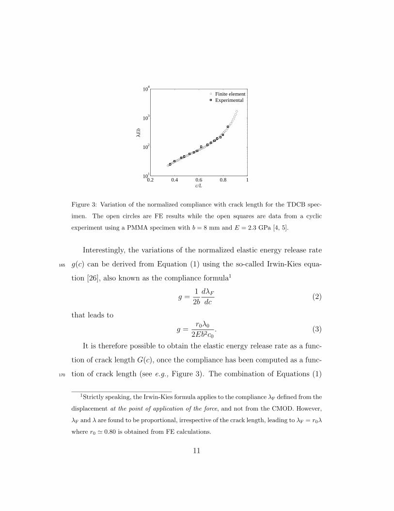
non-dimensional compliance λEb, where E is the material Young’s modu-155

lus and b the specimen thickness, is shown in Figure 3. For the range of

crack lengths L/3 . c . 2L/3, the compliance can be approximated by an

exponential function

λ =λ0Eb

ec/c0 (1)

where λ0 = 6.0 and c0 = 21 mm are fitting parameters. When the crack

is very close to the boundary, the compliance deviates from the exponential160

approximation. As shown in Figure 3, this behavior is confirmed experimen-

tally by measuring the specimen compliance for different crack lengths in a

cyclic TDCB experiment using PMMA [4, 5].

10

0.2 0.4 0.6 0.8 110

1

102

103

104

c/L

λEb

Finite elementExperimental

Figure 3: Variation of the normalized compliance with crack length for the TDCB spec-

imen. The open circles are FE results while the open squares are data from a cyclic

experiment using a PMMA specimen with b = 8 mm and E = 2.3 GPa [4, 5].

Interestingly, the variations of the normalized elastic energy release rate

g(c) can be derived from Equation (1) using the so-called Irwin-Kies equa-165

tion [26], also known as the compliance formula1

g =1

2b

dλFdc

(2)

that leads to

g =r0λ0

2Eb2c0. (3)

It is therefore possible to obtain the elastic energy release rate as a func-

tion of crack length G(c), once the compliance has been computed as a func-

tion of crack length (see e.g., Figure 3). The combination of Equations (1)170

1Strictly speaking, the Irwin-Kies formula applies to the compliance λF defined from the

displacement at the point of application of the force, and not from the CMOD. However,

λF and λ are found to be proportional, irrespective of the crack length, leading to λF = r0λ

where r0 ' 0.80 is obtained from FE calculations.

11

and (3) provides the elastic energy release rate G = F 2g(c) =δ2

λ(c)2g(c) un-

der displacement controlled conditions, leading to

G(c) = δ2r0E

2λ0c0e−c/c0. (4)

The exponential decay of G with crack length points out the high stability

of the fracture process of the modified TDCB geometry for displacement-

controlled loading conditions. Last, the mode I SIF derives from Irwin’s175

relationship [27] under plane stress condition

KI =√GE (5)

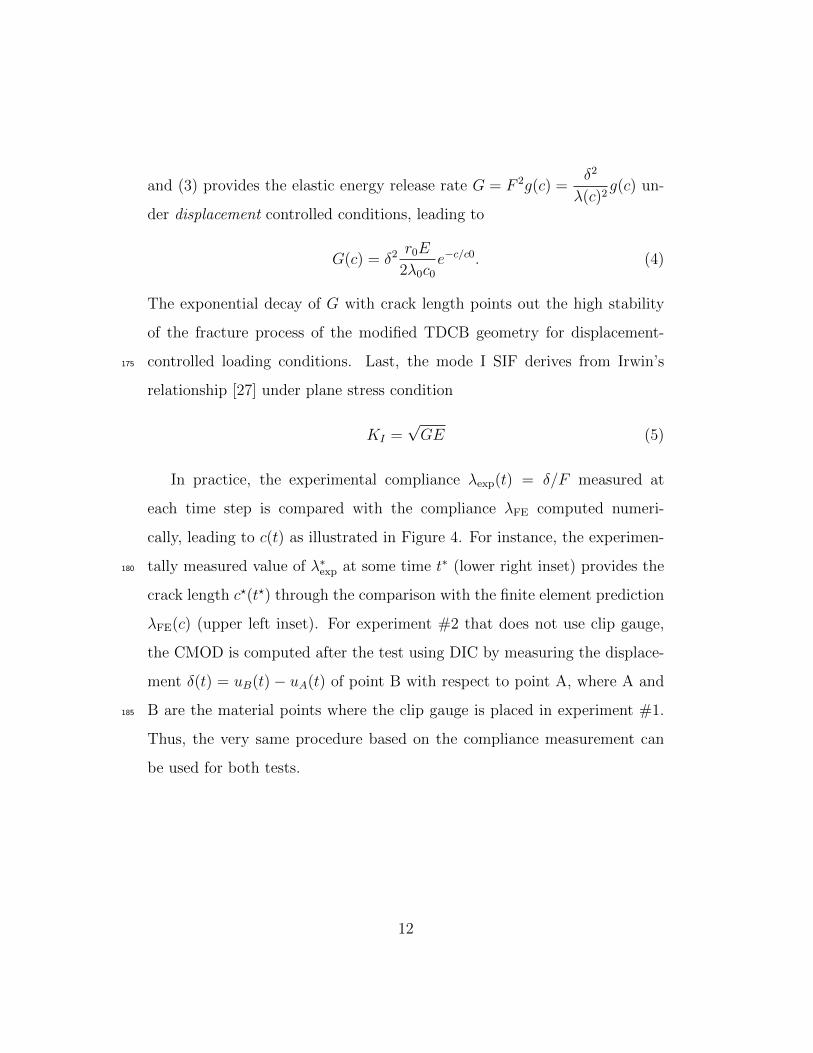
In practice, the experimental compliance λexp(t) = δ/F measured at

each time step is compared with the compliance λFE computed numeri-

cally, leading to c(t) as illustrated in Figure 4. For instance, the experimen-

tally measured value of λ∗exp at some time t∗ (lower right inset) provides the180

crack length c?(t?) through the comparison with the finite element prediction

λFE(c) (upper left inset). For experiment #2 that does not use clip gauge,

the CMOD is computed after the test using DIC by measuring the displace-

ment δ(t) = uB(t)− uA(t) of point B with respect to point A, where A and

B are the material points where the clip gauge is placed in experiment #1.185

Thus, the very same procedure based on the compliance measurement can

be used for both tests.

12

200 300 400 500 60055

60

65

70

75

80

85

90

95

t (s)

c (m

m)

cexp*

t*= 400

60 80 10010

2

103

c (mm)λE

b

λexp*

300 400 50010

2

103

t (s)

λEb

λexp*

t*= 400

λexp

Eb

λFE

Eb

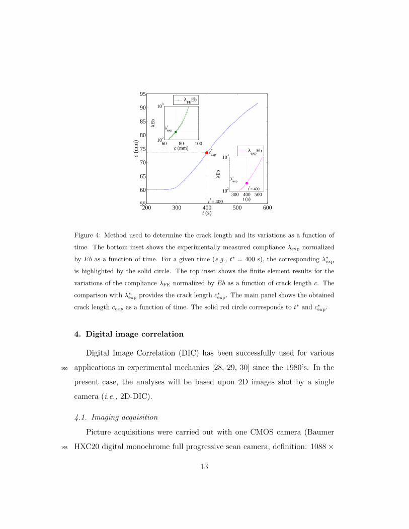
Figure 4: Method used to determine the crack length and its variations as a function of

time. The bottom inset shows the experimentally measured compliance λexp normalized

by Eb as a function of time. For a given time (e.g., t∗ = 400 s), the corresponding λ∗exp

is highlighted by the solid circle. The top inset shows the finite element results for the

variations of the compliance λFE normalized by Eb as a function of crack length c. The

comparison with λ∗exp provides the crack length c∗exp. The main panel shows the obtained

crack length cexp as a function of time. The solid red circle corresponds to t∗ and c∗exp.

4. Digital image correlation

Digital Image Correlation (DIC) has been successfully used for various

applications in experimental mechanics [28, 29, 30] since the 1980’s. In the190

present case, the analyses will be based upon 2D images shot by a single

camera (i.e., 2D-DIC).

4.1. Imaging acquisition

Picture acquisitions were carried out with one CMOS camera (Baumer

HXC20 digital monochrome full progressive scan camera, definition: 1088×195

13

2048 pixels). A Zeiss fixed lens (100 mm F2, model Makro-planar T*) and a

Nikon extension tube (52.5 mm, PN-11 model) were used. The pictures were

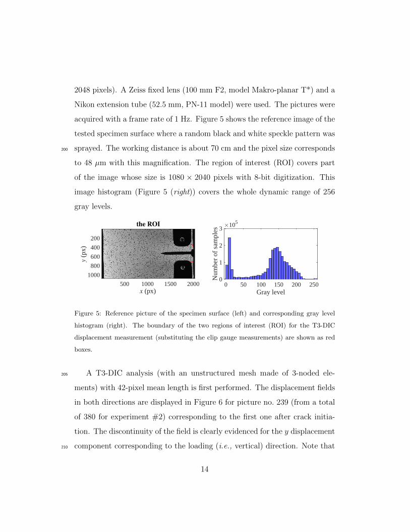
acquired with a frame rate of 1 Hz. Figure 5 shows the reference image of the

tested specimen surface where a random black and white speckle pattern was

sprayed. The working distance is about 70 cm and the pixel size corresponds200

to 48 µm with this magnification. The region of interest (ROI) covers part

of the image whose size is 1080 × 2040 pixels with 8-bit digitization. This

image histogram (Figure 5 (right)) covers the whole dynamic range of 256

gray levels.

the ROI

x (px)500 1000 1500 2000

y (

px)

200

400

600

800

1000

Gray level0 50 100 150 200 250

Num

ber

of s

ampl

es

×105

0

1

2

3

Figure 5: Reference picture of the specimen surface (left) and corresponding gray level

histogram (right). The boundary of the two regions of interest (ROI) for the T3-DIC

displacement measurement (substituting the clip gauge measurements) are shown as red

boxes.

A T3-DIC analysis (with an unstructured mesh made of 3-noded ele-205

ments) with 42-pixel mean length is first performed. The displacement fields

in both directions are displayed in Figure 6 for picture no. 239 (from a total

of 380 for experiment #2) corresponding to the first one after crack initia-

tion. The discontinuity of the field is clearly evidenced for the y displacement

component corresponding to the loading (i.e., vertical) direction. Note that210

14

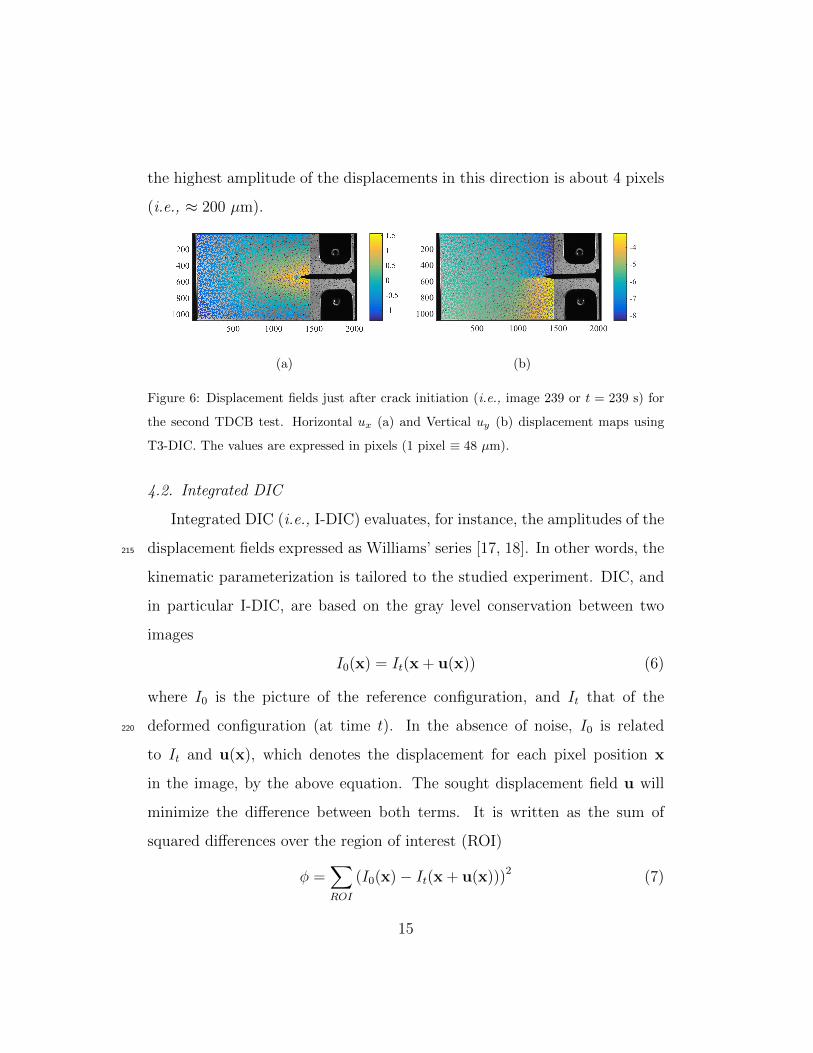
the highest amplitude of the displacements in this direction is about 4 pixels

(i.e., ≈ 200 µm).

(a) (b)

Figure 6: Displacement fields just after crack initiation (i.e., image 239 or t = 239 s) for

the second TDCB test. Horizontal ux (a) and Vertical uy (b) displacement maps using

T3-DIC. The values are expressed in pixels (1 pixel ≡ 48 µm).

4.2. Integrated DIC

Integrated DIC (i.e., I-DIC) evaluates, for instance, the amplitudes of the

displacement fields expressed as Williams’ series [17, 18]. In other words, the215

kinematic parameterization is tailored to the studied experiment. DIC, and

in particular I-DIC, are based on the gray level conservation between two

images

I0(x) = It(x + u(x)) (6)

where I0 is the picture of the reference configuration, and It that of the

deformed configuration (at time t). In the absence of noise, I0 is related220

to It and u(x), which denotes the displacement for each pixel position x

in the image, by the above equation. The sought displacement field u will

minimize the difference between both terms. It is written as the sum of

squared differences over the region of interest (ROI)

φ =∑ROI

(I0(x)− It(x + u(x)))2 (7)

15

The displacement fields u may be expressed with different parameteriza-225

tions. For example, a series of mechanically meaningful fields Ψi (e.g., Williams’

series) with unknown amplitudes υi (e.g., SIFs) as the sought parameters

u(x) =∑i

υiΨi(x) (8)

so that φ will depends on the column vector {υυυ} gathering all amplitudes υi.

4.2.1. Williams’ series

Assuming a crack path along the negative x-axis, and the crack tip posi-230

tion at the origin, the displacement fields read

u(z) =II∑j=I

pf∑n=pi

ωjnψψψ

jn(z) (9)

where the vector fields are defined in the complex plane

z = x+ iy = r exp(iθ) (10)

with, j = I for a mode I fracture regime

ψψψIn(z) =

A(n)

2µ√

2πr

n2

[κ exp

(inθ

2

)− n

2exp

(i(4− n)θ

2

)+(

(−1)n +n

2

)exp

(−inθ

2

)](11)

and j = II for a mode II regime

ψψψIIn (z) =

iA(n)

2µ√

2πr

n2

[κ exp

(inθ

2

)+n

2exp

(i(4− n)θ

2

)+(

(−1)n − n

2

)exp

(−inθ

2

)](12)

16

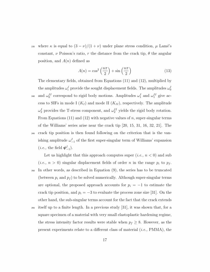
where κ is equal to (3 − ν)/(1 + ν) under plane stress condition, µ Lame’s235

constant, ν Poisson’s ratio, r the distance from the crack tip, θ the angular

position, and A(n) defined as

A(n) = cos2(nπ

2

)+ sin

(nπ2

)(13)

The elementary fields, obtained from Equations (11) and (12), multiplied by

the amplitudes ωji provide the sought displacement fields. The amplitudes ωI

0

and ωII0 correspond to rigid body motions. Amplitudes ωI

1 and ωII1 give ac-240

cess to SIFs in mode I (KI) and mode II (KII), respectively. The amplitude

ωI2 provides the T-stress component, and ωII

2 yields the rigid body rotation.

From Equations (11) and (12) with negative values of n, super-singular terms

of the Williams’ series arise near the crack tip [20, 15, 31, 16, 32, 21]. The

crack tip position is then found following on the criterion that is the van-245

ishing amplitude ωI−1 of the first super-singular term of Williams’ expansion

(i.e., the field ψψψI−1).

Let us highlight that this approach computes super (i.e., n < 0) and sub

(i.e., n > 0) singular displacement fields of order n in the range pi to pf .

In other words, as described in Equation (9), the series has to be truncated250

(between pi and pf ) to be solved numerically. Although super-singular terms

are optional, the proposed approach accounts for pi = −1 to estimate the

crack tip position, and pi = −3 to evaluate the process zone size [31]. On the

other hand, the sub-singular terms account for the fact that the crack extends

itself up to a finite length. In a previous study [31], it was shown that, for a255

square specimen of a material with very small elastoplastic hardening regime,

the stress intensity factor results were stable when pf ≥ 8. However, as the

present experiments relate to a different class of material (i.e., PMMA), the

17

influence of the number of terms will be studied.

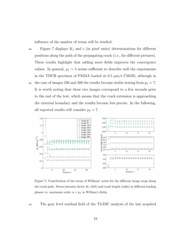
Figure 7 displays KI and c (in pixel units) determinations for different260

positions along the path of the propagating crack (i.e., for different pictures).

These results highlight that adding more fields improves the convergence

values. In general, pf = 5 seems sufficient to describe well the experiments

in the TDCB specimen of PMMA loaded at 0.5 µm/s CMOD, although in

the case of images 330 and 380 the results become stable staring from pf = 7.265

It is worth noting that these two images correspond to a few seconds prior

to the end of the test, which means that the crack extension is approaching

the external boundary and the results become less precise. In the following,

all reported results will consider pf = 7.

Positve n5 10 15 20

KI (

MPa

.m1/

2 )

0

0.2

0.4

0.6

0.8

1

1.2

1.4image 60image 90image 150image 200image 240image 290image 330image 380

Positve n5 10 15 20

480

500

520

540

5 10 15 20crac

k le

ngth

(pi

xel)

550630710790870950

5 10 15 201000

1100

1200

1300

Figure 7: Contribution of the terms of Williams’ series for the different image steps along

the crack path. Stress intensity factor KI (left) and crack length (right) at different loading

phases vs. maximum order n = pf in William’s fields.

The gray level residual field of the T3-DIC analysis of the last acquired270

18

image

η(x) = I0(x)− It(x + u(x)) (14)

allows for the precise identification of the cracked region [15] since the con-

tinuity enforced by triangular meshes is not satisfied across the crack mouth

(Figure 8). From this information, the crack path is visible (red dashed

line). The latter is used for all I-DIC calculations and the crack tip position275

along this straight path is then determined by canceling out the amplitude

ωI−1 [33, 21].

x (px)200 400 600 800 1000 1200 1400

y (

px)

300

400

500

600

700

800

900 -4

-3

-2

-1

0

1

2

3

Figure 8: Gray level residual map for the last image revealing the path followed by the crack

in the second experiment (1 pixel ≡ 48 µm). The dashed line represents the propagation

direction.

Figure 9 shows the displacement fields of the last loading step. There

is no clear displacement gradient along the crack direction of the horizon-

tal component. Conversely, there is a strong displacement gradient in the280

vertical direction. From this qualitative observation, it is expected that the

experiment is under dominant mode I condition. This observation will be

quantitatively confirmed via I-DIC.

19

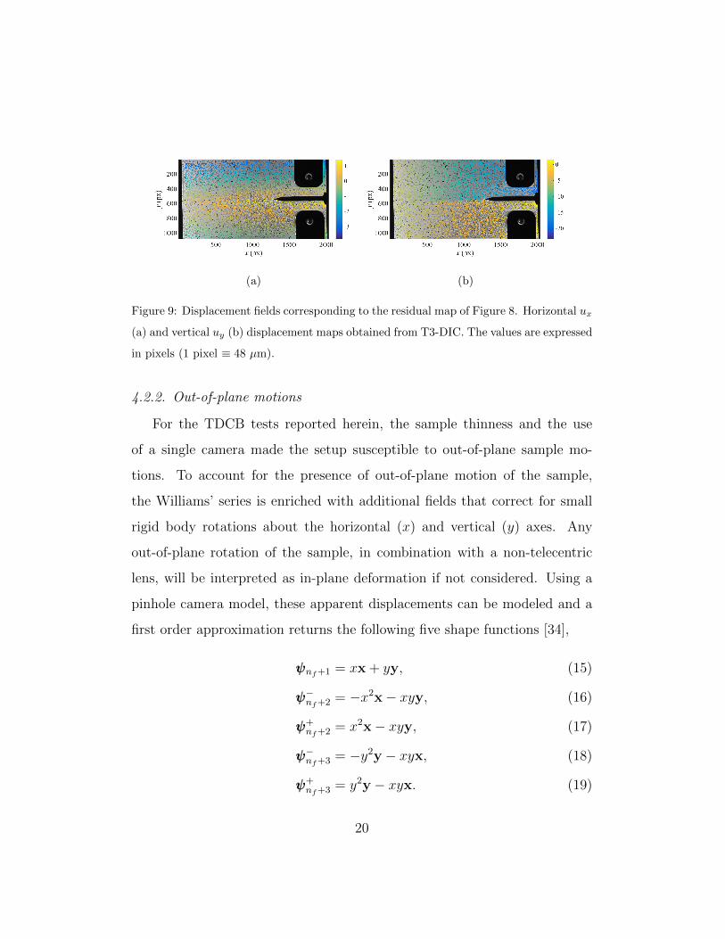
(a) (b)

Figure 9: Displacement fields corresponding to the residual map of Figure 8. Horizontal ux

(a) and vertical uy (b) displacement maps obtained from T3-DIC. The values are expressed

in pixels (1 pixel ≡ 48 µm).

4.2.2. Out-of-plane motions

For the TDCB tests reported herein, the sample thinness and the use

of a single camera made the setup susceptible to out-of-plane sample mo-

tions. To account for the presence of out-of-plane motion of the sample,

the Williams’ series is enriched with additional fields that correct for small

rigid body rotations about the horizontal (x) and vertical (y) axes. Any

out-of-plane rotation of the sample, in combination with a non-telecentric

lens, will be interpreted as in-plane deformation if not considered. Using a

pinhole camera model, these apparent displacements can be modeled and a

first order approximation returns the following five shape functions [34],

ψψψnf+1 = xx + yy, (15)

ψψψ−nf+2 = −x2x− xyy, (16)

ψψψ+nf+2 = x2x− xyy, (17)

ψψψ−nf+3 = −y2y − xyx, (18)

ψψψ+nf+3 = y2y − xyx. (19)

20

Equation (15) expresses magnification changes due to a translation along the285

optical axis. Equations (16)-(17) account for the apparent deformation for

negative and positive rotations respectively about the image vertical axis.

Likewise Equations (18)-(19) express the deformation to account for rotation

about the image horizontal direction. Thus, the description of all rigid body

motions along the system coordinates of the camera is defined by the five290

fields introduced above. It is worth recalling that Equation (9), which is

truncated between n = pi and pf , is solved numerically, to explain that in

this particular case these extra modes are added to the truncated series.

5. Results and discussion

In this section, both TDCB experiments are studied independently, com-295

paring the fracture properties obtained when using the method based on

compliance variations and the integrated DIC framework. Let us first high-

light the differences between both test configurations describing them in de-

tail. In the first case, the specimen geometry had its original crack length

(36.5 mm) modified by a laser cutting extension accompanied by a pre-load300

procedure of the sample, which yielded a TDCB specimen with cini = 60 mm.

Furthermore, the displacements were recorded by a clip gauge that also con-

trolled the fracture experiment at a constant crack mouth opening rate of

5 µm/s. In the second experiment no clip gauge was used and no pre-loading

was applied. The crack mouth opening displacements δ were measured via305

T3-DIC after the test. Figure 5 displays the two ROIs where δ was measured.

Once δ is obtained from DIC (instead of the clip gauge) and force-time data

(i.e., F (t)) are available, the compliance based method is applied as well.

21

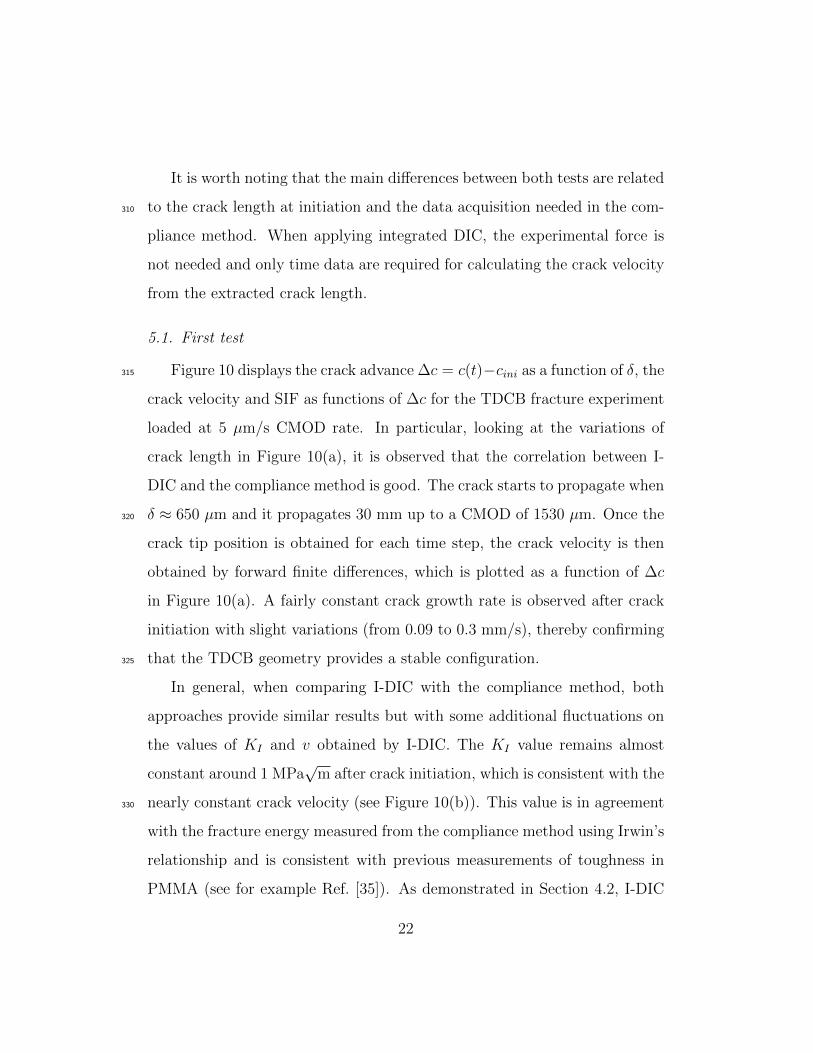
It is worth noting that the main differences between both tests are related

to the crack length at initiation and the data acquisition needed in the com-310

pliance method. When applying integrated DIC, the experimental force is

not needed and only time data are required for calculating the crack velocity

from the extracted crack length.

5.1. First test

Figure 10 displays the crack advance ∆c = c(t)−cini as a function of δ, the315

crack velocity and SIF as functions of ∆c for the TDCB fracture experiment

loaded at 5 µm/s CMOD rate. In particular, looking at the variations of

crack length in Figure 10(a), it is observed that the correlation between I-

DIC and the compliance method is good. The crack starts to propagate when

δ ≈ 650 µm and it propagates 30 mm up to a CMOD of 1530 µm. Once the320

crack tip position is obtained for each time step, the crack velocity is then

obtained by forward finite differences, which is plotted as a function of ∆c

in Figure 10(a). A fairly constant crack growth rate is observed after crack

initiation with slight variations (from 0.09 to 0.3 mm/s), thereby confirming

that the TDCB geometry provides a stable configuration.325

In general, when comparing I-DIC with the compliance method, both

approaches provide similar results but with some additional fluctuations on

the values of KI and v obtained by I-DIC. The KI value remains almost

constant around 1 MPa√

m after crack initiation, which is consistent with the

nearly constant crack velocity (see Figure 10(b)). This value is in agreement330

with the fracture energy measured from the compliance method using Irwin’s

relationship and is consistent with previous measurements of toughness in

PMMA (see for example Ref. [35]). As demonstrated in Section 4.2, I-DIC

22

allows the presence (or absence) of mode II regime to be evaluated. It is

found that KII remains very close to zero all along crack propagation. This335

observation is consistent with the criterion of local symmetry [36, 37, 38, 39]

that predicts crack propagation along a path that satisfies KII = 0 (here, a

straight path perpendicular to the loading axis).

∆c (mm)0 10 20 30

v (

m.s

-1)

10-6

10-5

10-4

10-3

(b)

compliance methodIDIC

δ (µm)500 1000 1500 2000

∆c (

mm

)

0

5

10

15

20

25

30(a)

compliance methodIDIC

∆c (mm)0 5 10 15 20 25 30

SIF

(MPa

.m1/

2 )

-0.5

0

0.5

1

1.5

2(c) K

I - compliance method

KI - IDIC + tilt terms

KI - IDIC no tilt terms

KII

- IDIC + tilt terms

Figure 10: Comparison between the compliance method and the I-DIC technique results

for the TDCB specimen tested with clip gauge. (a) Crack length as a function of CMOD,

(b) crack velocity as a function of crack length and (c) stress intensity factor as a function

of crack length.

5.2. Second test

Figure 11 displays crack length, crack velocity, and SIFs for the second340

experiment (controlled by the stroke speed of 2.5 µm/s). First, an unstable

23

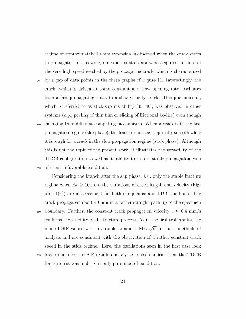
regime of approximately 10 mm extension is observed when the crack starts

to propagate. In this zone, no experimental data were acquired because of

the very high speed reached by the propagating crack, which is characterized

by a gap of data points in the three graphs of Figure 11. Interestingly, the345

crack, which is driven at some constant and slow opening rate, oscillates

from a fast propagating crack to a slow velocity crack. This phenomenon,

which is referred to as stick-slip instability [35, 40], was observed in other

systems (e.g., peeling of thin film or sliding of frictional bodies) even though

emerging from different competing mechanisms. When a crack is in the fast350

propagation regime (slip phase), the fracture surface is optically smooth while

it is rough for a crack in the slow propagation regime (stick phase). Although

this is not the topic of the present work, it illustrates the versatility of the

TDCB configuration as well as its ability to restore stable propagation even

after an unfavorable condition.355

Considering the branch after the slip phase, i.e., only the stable fracture

regime when ∆c > 10 mm, the variations of crack length and velocity (Fig-

ure 11(a)) are in agreement for both compliance and I-DIC methods. The

crack propagates about 40 mm in a rather straight path up to the specimen

boundary. Further, the constant crack propagation velocity v ≈ 0.4 mm/s360

confirms the stability of the fracture process. As in the first test results, the

mode I SIF values were invariable around 1 MPa√

m for both methods of

analysis and are consistent with the observation of a rather constant crack

speed in the stick regime. Here, the oscillations seen in the first case look

less pronounced for SIF results and KII ≈ 0 also confirms that the TDCB365

fracture test was under virtually pure mode I condition.

24

∆c (mm)0 10 20 30 40 50

v (

m.s

-1)

10-6

10-4

10-2

(b)

compliance methodIDIC

δ (µm)400 600 800 1000

∆c (

mm

)

0

10

20

30

40

50(a)

compliance methodIDIC

∆c (mm)0 10 20 30 40 50

SIF

(MPa

.m1/

2 )

-0.5

0

0.5

1

1.5

2 (c) KI - compliance method

KI - IDIC + tilt terms

KI - IDIC no tilt terms

KII

- IDIC + tilt terms

Figure 11: Comparison between the compliance method and the I-DIC technique results

for the TDCB specimen tested with no clip gauge. (a) Crack length as a function of

CMOD, (b) crack velocity as a function of crack length and (c) stress intensity factor as

a function of crack length.

5.3. Discussion

Figure 12 shows the changes of the root mean square gray level residuals

normalized by the dynamic range of the picture in the reference configuration

for the two phases of the test that could be monitored, namely, prior to370

initiation, and in the stable propagation regime. For instance, during the

first phase of the second test, these dimensionless residuals vary from 0.105

and 0.115 with an average value of 0.11. It is believed that the main reason for

these rather high values is due to lighting. In the present case two LED panels

25

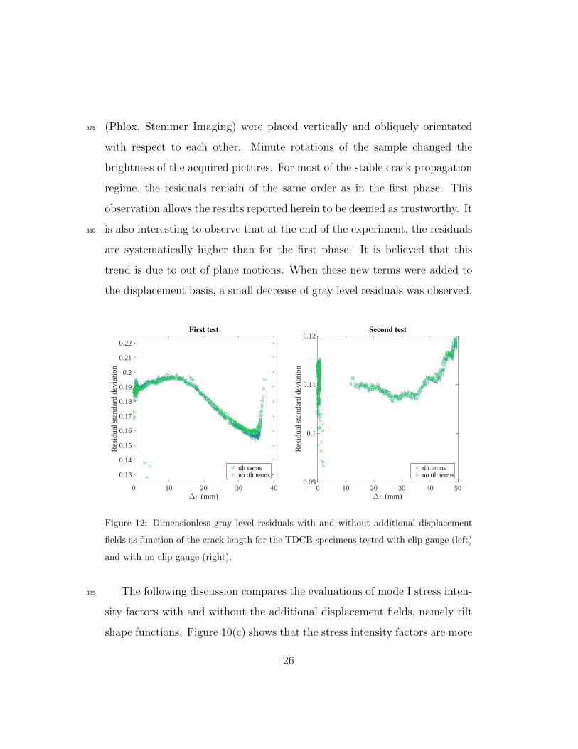
(Phlox, Stemmer Imaging) were placed vertically and obliquely orientated375

with respect to each other. Minute rotations of the sample changed the

brightness of the acquired pictures. For most of the stable crack propagation

regime, the residuals remain of the same order as in the first phase. This

observation allows the results reported herein to be deemed as trustworthy. It

is also interesting to observe that at the end of the experiment, the residuals380

are systematically higher than for the first phase. It is believed that this

trend is due to out of plane motions. When these new terms were added to

the displacement basis, a small decrease of gray level residuals was observed.

∆c (mm)0 10 20 30 40

Res

idua

l sta

ndar

d de

viat

ion

0.13

0.14

0.15

0.16

0.17

0.18

0.19

0.2

0.21

0.22

First test

tilt termsno tilt terms

∆c (mm)0 10 20 30 40 50

Res

idua

l sta

ndar

d de

viat

ion

0.09

0.1

0.11

0.12Second test

tilt termsno tilt terms

Figure 12: Dimensionless gray level residuals with and without additional displacement

fields as function of the crack length for the TDCB specimens tested with clip gauge (left)

and with no clip gauge (right).

The following discussion compares the evaluations of mode I stress inten-385

sity factors with and without the additional displacement fields, namely tilt

shape functions. Figure 10(c) shows that the stress intensity factors are more

26

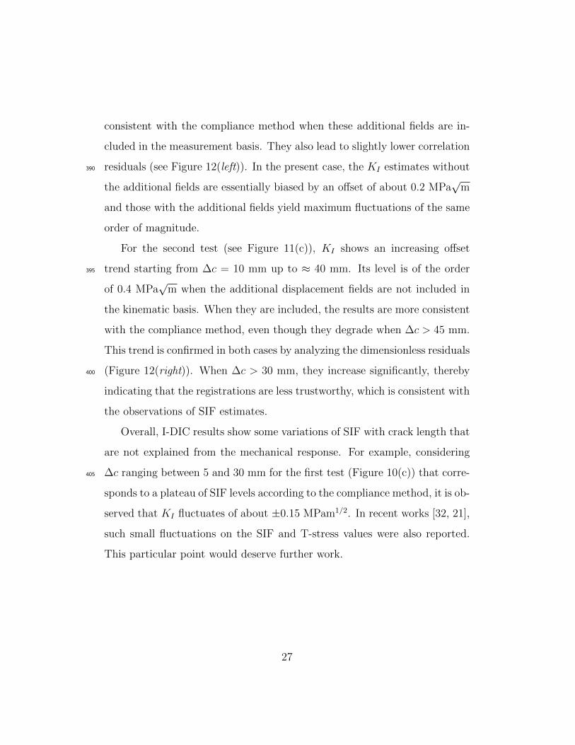
consistent with the compliance method when these additional fields are in-

cluded in the measurement basis. They also lead to slightly lower correlation

residuals (see Figure 12(left)). In the present case, the KI estimates without390

the additional fields are essentially biased by an offset of about 0.2 MPa√

m

and those with the additional fields yield maximum fluctuations of the same

order of magnitude.

For the second test (see Figure 11(c)), KI shows an increasing offset

trend starting from ∆c = 10 mm up to ≈ 40 mm. Its level is of the order395

of 0.4 MPa√

m when the additional displacement fields are not included in

the kinematic basis. When they are included, the results are more consistent

with the compliance method, even though they degrade when ∆c > 45 mm.

This trend is confirmed in both cases by analyzing the dimensionless residuals

(Figure 12(right)). When ∆c > 30 mm, they increase significantly, thereby400

indicating that the registrations are less trustworthy, which is consistent with

the observations of SIF estimates.

Overall, I-DIC results show some variations of SIF with crack length that

are not explained from the mechanical response. For example, considering

∆c ranging between 5 and 30 mm for the first test (Figure 10(c)) that corre-405

sponds to a plateau of SIF levels according to the compliance method, it is ob-

served that KI fluctuates of about ±0.15 MPam1/2. In recent works [32, 21],

such small fluctuations on the SIF and T-stress values were also reported.

This particular point would deserve further work.

27

6. Conclusion410

In this work, two tapered double cantilever beam experiments were dis-

cussed independently. The results show that the TDCB geometry adopted

herein induces stable fracture. In particular, it was highlighted in the sec-

ond test by its ability of restoring the slow (i.e., stable) crack propagation

regime even after being unintentionally introduced to a fast and unstable415

phenomenon at the initiation stage. All these observations validate the nu-

merical analyses performed to design such tests and confirm that this newly

developed fracture test geometry is appropriate to characterize the fracture

properties of brittle solids such as PMMA.

Integrated DIC was successfully used to analyze fracture mechanics pa-420

rameters (e.g., crack tip position, SIFs, mode mixity) of PMMA in experi-

ments using the TDCB geometry. In particular, it was shown that the tests

are mode I dominant, which was assumed a priori in the numerical simula-

tions. A comparison study between the I-DIC estimates and those obtained

with a method based on compliance variations showed that both approaches425

were consistent for both investigated tests. To achieve such agreements, it

was shown that global displacements describing out-of-plane rigid motions

had to be added to Williams’ kinematic basis. Another route, which would

be worth investigating in the future, would be to consider stereocorrelation

techniques to add more freedom to the out-of-plane kinematics [30].430

Overall, the integrated DIC analyses show promising results and appear

as a reliable method to determine fracture parameters in the TDCB configu-

ration. This paves the way to the characterization of the fracture behavior of

materials under extreme conditions where mechanical gauges may be limited

28

(e.g., at high temperatures or for fast propagation regimes). Let us note that435

this technique has already been successfully employed to determine fracture

properties of other brittle [18, 41, 21] or ductile [20, 16, 33, 32] materials.

One additional result of the present work was its validation against an inde-

pendent method.

Acknowledgments440

It is a pleasure to acknowledge the financial support of the Brazilian agen-

cies CNPq and CAPES to this investigation during the doctoral thesis and

postdoctoral study of TMG. TMG’s stay at UPMC and LMT was supported

by the Doctoral Sandwich Program Abroad (PDSE fellowship) of CAPES,

grant #99999.009821/2014− 07. This work was also partially supported by445

BPI France within the DICCIT project.

29

References

[1] ASTM E1820-17, Standard Test Method for Measurement of Fracture

Toughness, ASTM International, West Conshohocken, PA (USA), 2017.

[2] A. Shyam, E. Lara-Curzio, The double-torsion testing technique for de-450

termination of fracture toughness and slow crack growth behavior of

materials: A review, Journal of Materials Science 41 (13) (2006) 4093–

4104.

[3] H. Liebowitz, Fracture, vol. 5 Edition, Academic, New York, 1969.

[4] T. M. Grabois, Experimental fracture mechanics of cement-based mate-455

rials: A new methodology for the accurate measurement of the material

toughness, PhD thesis, Universidade Federal do Rio de Janeiro (2016).

[5] A. V. Vasudevan, T. M. Grabois, G. C. Cordeiro, R. D. Toledo Filho,

L. Ponson, A new fracture test methodology for the accurate character-

ization of brittle fracture properties, (in preparation).460

[6] J. P. Gallagher, Experimentally determined stress intensity factors for

several contoured double cantilever beam specimens, Engineering Frac-

ture Mechanics 3 (1) (1971) 27–43.

[7] H. L. Marcus, G. C. Sih, A crackline-loaded edge-crack stress corrosion

specimen, Engineering Fracture Mechanics 3 (4) (1971) 453–461.465

[8] J. F. Davalos, P. Madabhusi-Raman, P. Z. Qiao, M. P. Wolcott, Compli-

ance rate change of tapered double cantilever beam specimen with hy-

30

brid interface bonds, Theoretical and Applied Fracture Mechanics 29 (2)

(1998) 125–139.

[9] J.-L. Coureau, S. Morel, N. Dourado, Cohesive zone model and quasib-470

rittle failure of wood: A new light on the adapted specimen geometries

for fracture tests, Engineering Fracture Mechanics 109 (0) (2013) 328–

340.

[10] P. Qiao, J. Wang, J. F. Davalos, Tapered beam on elastic foundation

model for compliance rate change of TDCB specimen, Engineering Frac-475

ture Mechanics 70 (2) (2003) 339–353.

[11] B. R. K. Blackman, H. Hadavinia, A. J. Kinloch, M. Paraschi, J. G.

Williams, The calculation of adhesive fracture energies in mode I: re-

visiting the tapered double cantilever beam (TDCB) test, Engineering

Fracture Mechanics 70 (2) (2003) 233–248.480

[12] S. McNeill, W. Peters, M. Sutton, Estimation of stress intensity factor by

digital image correlation, Engineering Fracture Mechanics 28 (1) (1987)

101–112.

[13] J. Abanto-Bueno, J. Lambros, Investigation of crack growth in func-

tionally graded materials using digital image correlation, Engineering485

Fracture Mechanics 69 (2002) 1695–1711.

[14] P. Forquin, L. Rota, Y. Charles, F. Hild, A method to determine the

toughness scatter of brittle materials, International Journal of Fracture

125 (1) (2004) 171–187.

31

[15] S. Roux, J. Rethore, F. Hild, Digital Image Correlation and Fracture:490

An Advanced Technique for Estimating Stress Intensity Factors of 2D

and 3D Cracks, Journal of Physics D: Applied Physics 42 (2009) 214004.

[16] F. Mathieu, F. Hild, S. Roux, Identification of a crack propagation law

by digital image correlation, International Journal of Fatigue 36 (1)

(2012) 146–154.495

[17] M. L. Williams, On the stress distribution at the base of a stationary

crack, Journal of Applied Mechanics 24 (1) (1957) 109–114.

[18] S. Roux, F. Hild, Stress intensity factor measurements from digital image

correlation: post-processing and integrated approaches, International

Journal of Fracture 140 (1-4) (2006) 141–157.500

[19] M. Y. Dehnavi, S. Khaleghian, A. Emami, M. Tehrani, N. Soltani, Utiliz-

ing digital image correlation to determine stress intensity factors, Poly-

mer Testing 37 (2014) 28–35.

[20] R. Hamam, F. Hild, S. Roux, Stress intensity factor gauging by digital

image correlation: Application in cyclic fatigue, Strain 43 (2007) 181–505

192.

[21] R. Vargas, J. Neggers, R. Canto, J. Rodrigues, F. Hild, Analysis of

wedge splitting test on refractory castable via integrated DIC, Journal

of the European Ceramic Society 36 (16) (2016) 4309–4317.

[22] S. Lampman, Characterization and failure analyses of plastics, ASM510

International, Materials Park, Ohio, 2003.

32

[23] H. Leclerc, J. Perie, S. Roux, F. Hild, Integrated digital image corre-

lation for the identification of mechanical properties, Vol. LNCS 5496,

Springer, Berlin (Germany), 2009, pp. 161–171.

[24] S. Morel, G. Mourot, J. Schmittbuhl, Influence of the specimen geometry515

on R-curve behavior and roughening of fracture surfaces, International

Journal of Fracture 121 (2003) 23–42.

[25] CAST3M, Finite Element package developed by CEA, France:

http://www-cast3m.cea.fr/index.php (version 2015).

[26] M. Kanninen, C. Popelar, Advanced Fracture Mechanics, Oxford Uni-520

versity Press, Oxford (UK), 1985.

[27] B. Lawn, Fracture of brittle solids, 2nd Edition, Cambridge University

Press, Cambridge, 1993.

[28] T. Chu, W. Ranson, M. Sutton, Applications of digital-image-correlation

techniques to experimental mechanics, Experimental Mechanics 25 (3)525

(1985) 232–244.

[29] M. Sutton, C. Mingqi, W. Peters, Y. Chao, S. McNeill, Application of

an optimized digital correlation method to planar deformation analysis,

Image and Vision Computing 4 (3) (1986) 143–150.

[30] M. Sutton, Computer vision-based, noncontacting deformation measure-530

ments in mechanics: A generational transformation, Applied Mechanics

Reviews 65 (AMR-13-1009, 050802).

33

[31] C. Henninger, S. Roux, F. Hild, Enriched kinematic fields of cracked

structures, International Journal of Solids and Structures 47 (24) (2010)

3305–3316.535

[32] J. Rethore, Automatic crack tip detection and stress intensity factors

estimation of curved cracks from digital images, International Journal

for Numerical Methods in Engineering 103 (7) (2015) 516–534.

[33] F. Mathieu, F. Hild, S. Roux, Image-based identification procedure of

a crack propagation law, Engineering Fracture Mechanics 103 (2013)540

48–59.

[34] J. Le Flohic, V. Parpoil, S. Bouissou, M. Poncelet, H. Leclerc, A 3D

Displacement Control by Digital Image Correlation for the Multiaxial

Testing of Materials with a Stewart Platform, Experimental Mechanics

54 (5) (2014) 817–828.545

[35] G. P. Marshall, L. H. Coutts, J. G. Williams, Temperature effects in the

fracture of PMMA, Journal of Material Science 9 (1974) 1409–1419.

[36] R. V. Gol’dstein, R. L. Salganik, Brittle fracture of solids with arbitrary

cracks, International Journal of Fracture 10 (1974) 507–523.

[37] M. Amestoy, H. Bui, K. Dang Van, Deviation infinitesimale d’une fis-550

sure dans une direction arbitraire, Comptes Rendus de l’Academie des

Sciences Paris t. 289 (Serie B) (1979) 99–103.

[38] B. Cotterell, J. R. Rice, Slightly curved or kinked cracks, International

Journal of Fracture 16 (1980) 155–169.

34

[39] M. Amestoy, H. Bui, K. Dang Van, Analytic asymptotic solution of555

the kinked crack problem, in: D. Francois (Ed.), Proceedings of ICF5,

Vol. 1, Pergamon Press, 1981, pp. 107–113.

[40] K. Ravi-Chandar, M. Balzano, On the mechanics and mechanisms of

crack growth in polymeric materials, Engineering Fracture Mechanics

30 (5) (1988) 713–727.560

[41] J. Rethore, S. Roux, F. Hild, An extended and integrated digital image

correlation technique applied to the analysis of fractured samples. The

equilibrium gap method as a mechanical filter, European Journal of

Computational Mechanics 18 (3-4) (2009) 285–306.

35