On the structure of Langmuir turbulence

Article

Accepted Version

Teixeira, M.A.C. and Belcher, S. E. (2010) On the structure of Langmuir turbulence. Ocean modelling, 31 (3-4). pp. 105-119. ISSN 1463-5003 doi: https://doi.org/10.1016/j.ocemod.2009.10.007 Available at http://centaur.reading.ac.uk/16602/

It is advisable to refer to the publisher’s version if you intend to cite from the work. See Guidance on citing .

To link to this article DOI: http://dx.doi.org/10.1016/j.ocemod.2009.10.007

Publisher: Elsevier

All outputs in CentAUR are protected by Intellectual Property Rights law, including copyright law. Copyright and IPR is retained by the creators or other copyright holders. Terms and conditions for use of this material are defined in the End User Agreement .

www.reading.ac.uk/centaur

CentAUR

Central Archive at the University of Reading

Reading’s research outputs online

On the structure of Langmuir turbulence

M. A. C. Teixeiraa,∗, S. E. Belcherb

aUniversity of Lisbon, CGUL, IDL, Lisbon, PortugalbDepartment of Meteorology, University of Reading, Reading, UK

Abstract

The Stokes drift induced by surface waves distorts turbulence in the wind-

driven mixed layer of the ocean, leading to the development of streamwise

vortices, or Langmuir circulations, on a wide range of scales. We inves-

tigate the structure of the resulting Langmuir turbulence, and contrast it

with the structure of shear turbulence, using rapid distortion theory (RDT)

and kinematic simulation of turbulence. Firstly, these linear models show

clearly why elongated streamwise vortices are produced in Langmuir turbu-

lence, when Stokes drift tilts and stretches vertical vorticity into horizontal

vorticity, whereas elongated streaky structures in streamwise velocity fluctu-

ations (u) are produced in shear turbulence, because there is a cancellation

in the streamwise vorticity equation and instead it is vertical vorticity that is

amplified. Secondly, we develop scaling arguments, illustrated by analysing

data from LES, that indicate that Langmuir turbulence is generated when

the deformation of the turbulence by mean shear is much weaker than the

deformation by the Stokes drift. These scalings motivate a quantitative RDT

∗Corresponding author: M. A. C. Teixeira, Centro de Geofısica da Universidade deLisboa, Edifıcio C8, Campo Grande, 1749-016 Lisbon, Portugal

Email addresses: mateixeira@fc.ul.pt (M. A. C. Teixeira)

Preprint submitted to Ocean Modelling October 13, 2009

model of Langmuir turbulence that accounts for deformation of turbulence

by Stokes drift and blocking by the air–sea interface that is shown to yield

profiles of the velocity variances (u2, v2, w2) in good agreement with LES.

The physical picture that emerges, at least in the LES, is as follows. Early

in the life cycle of a Langmuir eddy initial turbulent disturbances of verti-

cal vorticity are amplified algebraically by the Stokes drift into elongated

streamwise vortices, the Langmuir eddies. The turbulence is thus in a near

two-component state, with u2 suppressed and v2 ≈ w2. Near the surface,

over a depth of order the integral length scale of the turbulence, the vertical

velocity (w) is brought to zero by blocking of the air–sea interface. Since the

turbulence is nearly two-component, this vertical energy is transfered into

the spanwise fluctuations, considerably enhancing v2 at the interface. After

a time of order half the eddy decorrelation time the nonlinear processes, such

as distortion by the strain field of the surrounding eddies, arrest the defor-

mation and the Langmuir eddy decays. Presumably, Langmuir turbulence

then consists of a statistically steady state of such Langmuir eddies. The

analysis then provides a dynamical connection between the flow structures

in LES of Langmuir turbulence and the dominant balance between Stokes

production and dissipation in the turbulent kinetic energy budget, found by

previous authors.

Key words: Langmuir circulation, Turbulence, Stokes drift, Mixed layer,

Rapid distortion theory

2

1. Introduction

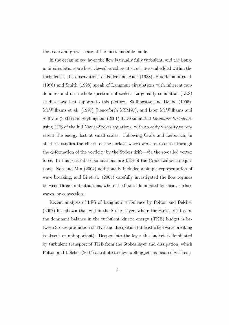
The velocity field in the surface mixed layer of the ocean is often dom-

inated by longitudinal vortices, known as Langmuir circulations, which are

aligned roughly with the wind, as reviewed by Leibovich (1983), Garrett

(1996) and Thorpe (2004). Direct observations (Pluddemann et al., 1996;

Smith, 1998; D’Asaro, 2001) and laboratory experiments (Faller and Cartwright,

1983; Nepf and Monismith, 1991; Melville et al., 1998) have shown that these

circulations play a key role in the transport and mixing of momentum, heat,

pollutants and dissolved gases from the surface into the deeper ocean (Kan-

tha and Clayson, 2004; McWilliams and Sullivan, 2001), and also in the

dispersion of buoyant tracers trapped at the surface (Faller and Auer, 1988;

Thorpe, 2001).

Craik and Leibovich (1976) and later Craik (1977), Leibovich (1977,

1980), Leibovich and Radhakrishnan (1977) and Leibovich and Paolucci

(1981) developed the established model for growth of Langmuir circulations

from small flow perturbations, namely an instability of the wind-induced

shear current to the Stokes drift associated with the surface waves. Accord-

ing to this mechanism (known as CL2) the Stokes drift tilts and amplifies

the vertical vorticity associated with any small spanwise variations of the

shear current. This amplified vorticity then further amplifies the pertur-

bation to the wind-induced shear flow, leading to instability. The Craik-

Leibovich analysis, and the body of work that has grown from it (see Lei-

bovich, 1983; Thorpe, 2004), is concerned with the initiation of Langmuir

circulations within a flow where any existing turbulence has a purely diffu-

sive effect, and yields the spatial structure of the unstable normal modes and

3

the scale and growth rate of the most unstable mode.

In the ocean mixed layer the flow is usually fully turbulent, and the Lang-

muir circulations are best viewed as coherent structures embedded within the

turbulence: the observations of Faller and Auer (1988), Pluddemann et al.

(1996) and Smith (1998) speak of Langmuir circulations with inherent ran-

domness and on a whole spectrum of scales. Large eddy simulation (LES)

studies have lent support to this picture. Skillingstad and Denbo (1995),

McWilliams et al. (1997) (henceforth MSM97), and later McWilliams and

Sullivan (2001) and Skyllingstad (2001), have simulated Langmuir turbulence

using LES of the full Navier-Stokes equations, with an eddy viscosity to rep-

resent the energy lost at small scales. Following Craik and Leibovich, in

all these studies the effects of the surface waves were represented through

the deformation of the vorticity by the Stokes drift—via the so-called vortex

force. In this sense these simulations are LES of the Craik-Leibovich equa-

tions. Noh and Min (2004) additionally included a simple representation of

wave breaking, and Li et al. (2005) carefully investigated the flow regimes

between three limit situations, where the flow is dominated by shear, surface

waves, or convection.

Recent analysis of LES of Langmuir turbulence by Polton and Belcher

(2007) has shown that within the Stokes layer, where the Stokes drift acts,

the dominant balance in the turbulent kinetic energy (TKE) budget is be-

tween Stokes production of TKE and dissipation (at least when wave breaking

is absent or unimportant). Deeper into the layer the budget is dominated

by turbulent transport of TKE from the Stokes layer and dissipation, which

Polton and Belcher (2007) attribute to downwelling jets associated with con-

4

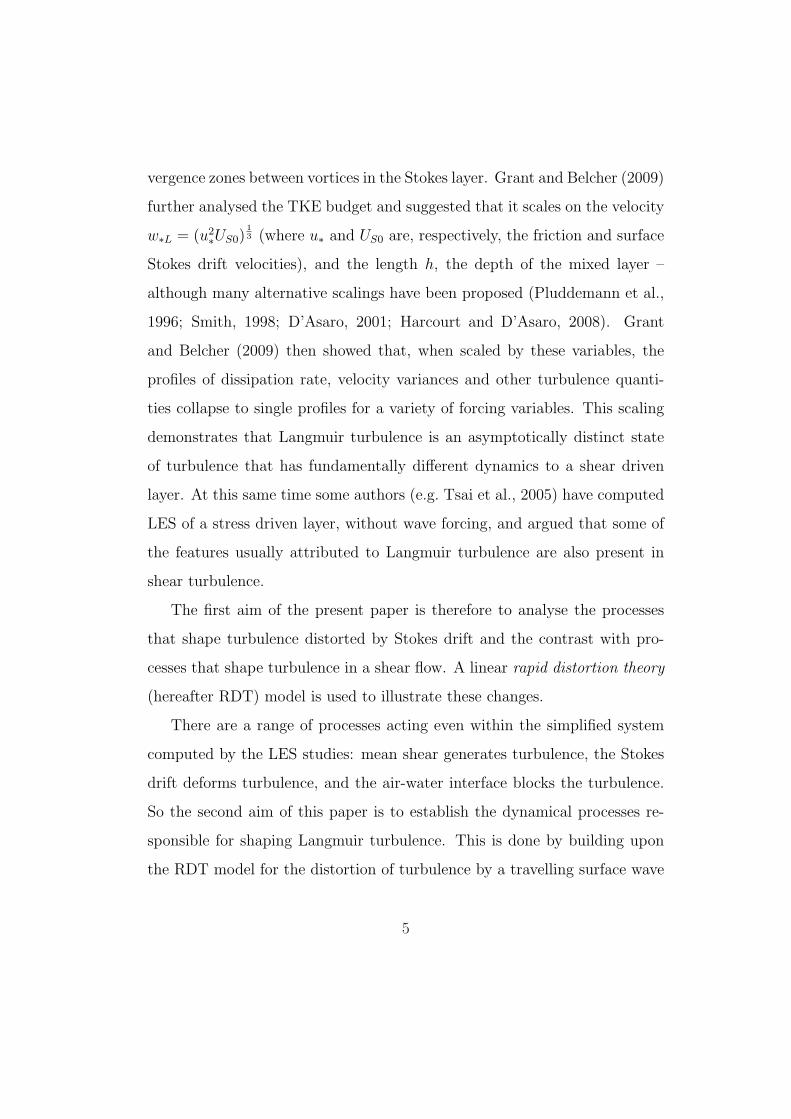
vergence zones between vortices in the Stokes layer. Grant and Belcher (2009)

further analysed the TKE budget and suggested that it scales on the velocity

w∗L = (u2∗US0)

13 (where u∗ and US0 are, respectively, the friction and surface

Stokes drift velocities), and the length h, the depth of the mixed layer –

although many alternative scalings have been proposed (Pluddemann et al.,

1996; Smith, 1998; D’Asaro, 2001; Harcourt and D’Asaro, 2008). Grant

and Belcher (2009) then showed that, when scaled by these variables, the

profiles of dissipation rate, velocity variances and other turbulence quanti-

ties collapse to single profiles for a variety of forcing variables. This scaling

demonstrates that Langmuir turbulence is an asymptotically distinct state

of turbulence that has fundamentally different dynamics to a shear driven

layer. At this same time some authors (e.g. Tsai et al., 2005) have computed

LES of a stress driven layer, without wave forcing, and argued that some of

the features usually attributed to Langmuir turbulence are also present in

shear turbulence.

The first aim of the present paper is therefore to analyse the processes

that shape turbulence distorted by Stokes drift and the contrast with pro-

cesses that shape turbulence in a shear flow. A linear rapid distortion theory

(hereafter RDT) model is used to illustrate these changes.

There are a range of processes acting even within the simplified system

computed by the LES studies: mean shear generates turbulence, the Stokes

drift deforms turbulence, and the air-water interface blocks the turbulence.

So the second aim of this paper is to establish the dynamical processes re-

sponsible for shaping Langmuir turbulence. This is done by building upon

the RDT model for the distortion of turbulence by a travelling surface wave

5

developed by Teixeira and Belcher (2002) (henceforth TB2002), and making

quantitative comparisons with the results of LES. We will find that the lin-

earised rapid-distortion approach explains both qualitative and quantitative

features of Langmuir turbulence. In this sense we seek here to provide a dy-

namical connection between the results from the TKE budget and the flow

structures observed in Langmuir turbulence.

The remainder of the paper is organised as follows. In Section 2, we begin

by introducing the formulation of the RDT model and contrasting the flow

structure predicted by kinematic simulation of turbulence (KST) for shear

turbulence and turbulence distorted by a surface wave. In Section 3 we

develop scalings for Langmuir turbulence through examination of the results

from the LES of MSM97. These scalings motivate a specific quantitative

comparison with RDT and KST. The ensuing results are presented in Section

4. Finally, the main conclusions of this study are presented in Section 5.

2. Rapid distortion and kinematic simulation of Langmuir turbu-

lence

In RDT, the equations of motion are linearised with respect to the turbu-

lent quantities (Batchelor and Proudman, 1954). Some turbulence is assumed

to exist initially, which is distorted for a finite time by an external forcing

(e.g. the Stokes drift of a wave) according to the linear dynamics. A final

turbulence state is thus obtained. This approach has been used previously

for shear flows by Townsend (1970), Lee and Hunt (1989), Lee et al. (1990)

and Mann (1994), and for blocking by rigid boundaries by Hunt and Graham

(1978) and Magnaudet (2003), for example. The limitations and assumptions

6

underlying RDT have been reviewed by Batchelor and Proudman (1954) and

Hunt (1973). Essentially, since RDT neglects nonlinear interactions in the

turbulence, it is approximately valid in situations when the velocity scale and

strain rate of the mean distorting flow are considerably larger than those of

the turbulence (i.e. weak turbulence).

For an incompressible and non-rotating fluid at high Reynolds number,

the linearised momentum and mass conservation equations may then be writ-

ten

∂u

∂t+ U · ∇u + u · ∇U =

1

ρ∇p, (1)

∇ · u = 0, (2)

where u is the turbulent velocity, p is the turbulent pressure, U is the mean

velocity, ρ is the density and ∇ is the spatial gradient operator. Mixing

by small-scale eddies could be taken into account through the inclusion of a

constant eddy viscosity in (1), as in Townsend (1970). However, the results

for the large-scale eddies, which are what concerns us here, would not be

appreciably changed, hence viscosity is ignored.

The evolution of turbulence statistics due to purely external forcings (in

this case the gradients of U, or the effect of boundaries) is determined by

adopting a spectral description of the flow (which allows elimination of the

pressure perturbation) and assuming an initial energy spectrum for the tur-

bulence. The turbulence is assumed to be locally homogeneous, and the mean

velocity gradients are assumed to be locally uniform (Hunt, 1973; Durbin,

1981; Hunt et al., 1990).

A spatial scale-separation between the turbulence and the mean flow

quantities is assumed, so that an average over a local volume V (x) can be

7

conceptually defined that yields, for example, the mean flow (by averaging

over the turbulent part):

U(x, t) =1

V (x)

∫∫∫v(x, t) dx dy dz, (3)

where v is total velocity, including mean and turbulent parts. Then a local

turbulent spectrum can be defined, formed over the same moving-average

volume, with slowly varying wavenumbers k(x, t) = (k1, k2, k3) and Fourier

coefficients u(H)(k,x, t) of the flow:

u(H) =1

(2π)3

∫∫∫u(H)e−ik·x dx dy dz. (4)

In this equation and in (3), the integration is carried out over the volume V

(see Hunt, 1973), and the superscript (H) denotes the flow away from any

boundaries. The corresponding turbulent velocity may be expressed by the

inverse Fourier transform:

u(H) =

∫∫∫u(H)eik·xdk1dk2dk3. (5)

Note that both u(H) and k are assumed to be slow functions of the spatial

coordinates (changing appreciably only over several wavelengths). Addition-

ally, not only is u(H) a function of time, satisfying an equation that results

from (1) in spectral space, but k also evolves in time, according to the equa-

tion (Dubrulle et al., 2004; Teixeira and Belcher, 2006)

∂k

∂t+∇ (k ·U) = 0. (6)

The approach followed here is essentially the same as described in detail in

Teixeira and Belcher (2002).

8

The presence of a rigid boundary acts to block the turbulence at the

surface, so that the normal component of the fluctuating velocity (w) is

brought to zero at the interface. Following Hunt and Graham (1978) this

process is represented over short times by adding to the flow within the fluid

the irrotational flow induced by image vortices above the interface, namely

u(t = 0) = u(H) +∇φ(S)(t = 0). (7)

Here φ(S) is a velocity potential, associated with the image vortices induced

by the interface to ensure no deformation of the interface by the turbulence.

This correction remains irrotational if the distorting flow is irrotational (e.g.

a surface wave). If the distorting flow possesses vorticity (e.g. shear), the

correction ceases to be irrotational over time.

KST (see Turfus and Hunt, 1987; Perkins et al., 1990; Fung et al., 1992),

goes one step further beyond RDT by providing actual realisations of turbu-

lent flows. This is particularly useful for tracking the trajectories of tracer

particles or calculating Lagrangian statistics. Turbulence is represented as

the sum of a discrete set of Fourier modes, with a random phase added to

each mode, while at the same time satisfying a given energy spectrum. The

constraint of incompressibility, (2), is enforced by calculating the velocity

field as the curl of another vector field, so that its divergence is zero. Hence,

for example, the turbulent velocity far from any boundary is represented as

u(H) =∑

n

[an cos(kn · x) + bn sin(kn · x)] , (8)

where

an = an × kn, bn = bn × kn, n = 1, 2, ... (9)

9

are Fourier amplitudes, kn are wavenumber vectors and n is the number of

the mode. kn = kn/|kn| are normalised vectors with the same direction

as the wavenumber kn and an and bn are vectors with the same modulus

as an and bn, respectively. The directions of kn, an and bn are picked from

random distributions. Additionally, the values of an and bn are picked from a

Gaussian distribution consistent with the prescribed energy spectrum. In the

calculations that follow, 300 Fourier modes, corresponding to 300 different

wavenumber values and directions will be considered.

The initial state of the turbulence is taken here to be isotropic, and with

the von Karman energy spectrum,

E(k0) = q2lg2(k0l)

4

(g1 + (k0l)2)176

, (10)

where k0 is the initial wavenumber magnitude, g1 and g2 are dimensionless

constants, q is the root-mean-square turbulent velocity and l is the longi-

tudinal length scale of the initial turbulence. In practice, this spectrum is

truncated at k0l = 5 in the KST results of this section in order to realistically

eliminate small scales in the turbulence and reduce noise (this mimics the

effect of a finite Reynolds number – see Teixeira and Belcher, 2000).

Two types of distorting mean flow are considered here: firstly a constant-

shear flow aligned in the x−direction,

U = αz, V = 0, (11)

where α is the shear rate. The total distortion, or total strain, to the tur-

bulence is then characterised by the dimensionless time β = αt. Secondly,

we consider the distortion due to the mean velocity that corresponds to an

10

irrotational wave propagating in the x direction, which may be written

U = awkwcwekwz cos(kwx− σwt),

W = awkwcwekwz sin(kwx− σwt), (12)

where aw, kw, cw and σw = cwkw are, respectively, the wave amplitude,

wavenumber, phase speed and angular frequency. In fact, as shown by

TB2002, what is relevant for the distortion of the turbulence over time in-

tervals longer than a wave period is the vertical gradient of the Stokes drift

of the wave, which is steady and given by

αS =dUS

dz= 2(awkw)2σwe2kwz, (13)

and for that reason the total distortion to the turbulence is characterised

by the dimensionless time βS = αSt. It can be shown that the linearised

wave-averaged vorticity equation that the turbulent motion must satisfy in

this case is

∂ω/∂t + US · ∇ω = ω · ∇US, (14)

where the systematic straining by the Stokes drift has been included. ω is

the turbulent vorticity and US is the Stokes drift velocity. This equation can

be obtained by taking the curl of the linearised Craik-Leibovich momentum

equation containing a vortex-force, and is thus essentially equivalent to it.

The solutions for k and u(H) that result from (6) and from the equation

that is obtained from inserting (5) into (1) are given, for the shear flow (11)

by e.g. Lee et al. (1990) and for the wave flow (12) by TB2002.

2.1. Shear and wave-distorted turbulence

Before RDT and KST are compared quantitatively with LES of Langmuir

turbulence, the structure of shear turbulence and turbulence distorted by an

11

irrotational surface wave will be contrasted.

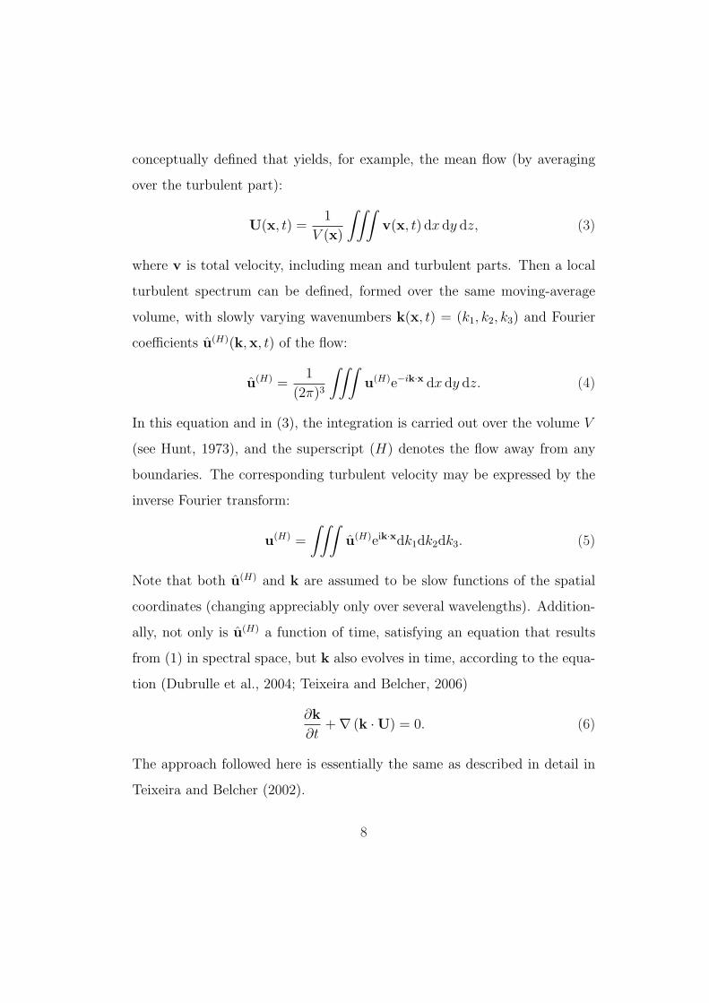
Fig. 1 shows cross-sections, at a depth z/l = 10, of the streamwise (u),

spanwise (v) and vertical (w) velocity fluctuations for turbulence distorted

by the constant-shear flow (11), after being distorted by this flow for a di-

mensionless time β = 5. This value is used for purely illustrative purposes,

since it allows a distinctive turbulence anisotropy to develop, being neverthe-

less not too different from values of the same parameter used in other RDT

studies (e.g. Lee et al., 1990; Mann, 1994).

An air-water interface is assumed to exist at z = 0 and the Froude number

of the turbulence is assumed to be so low that the turbulence does not deform

the interface. The depth chosen is such that influence from the boundary is

insignificant. As can be seen, v and especially u have large magnitude, while

w is considerably weaker. The ordering of the magnitudes of the velocity fluc-

tuations is u2 > v2 > w2, and the u velocity fluctuations are also elongated

along x, as is typical of shear-driven boundary layers. This flow structure is

similar to that presented in the RDT study of Lee et al. (1990) and in the

direct numerical simulations (DNS) of Tsai et al. (2005).

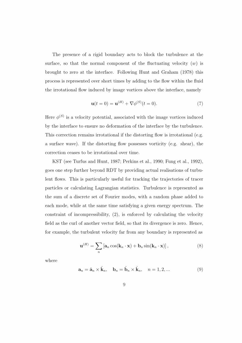
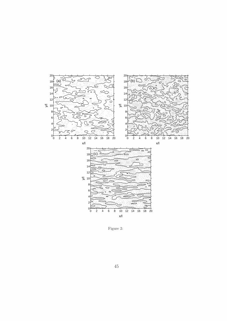
Fig. 2 shows cross-sections of the components of the velocity fluctuations

for turbulence distorted by a surface wave, as in TB2002, (12). In Fig. 2,

a wave of slope akkw = 0.2 and a time normalised by the wave period of

t/T = 10 has been assumed (as in TB2002), so that the dimensionless time

is βS = 5, similarly to Fig. 1. kwl has also been assumed to be zero, which

ensures that αS is effectively constant with depth (as α was in Fig. 1). This

is done here to facilitate the comparison, but would correspond in reality to

very long surface waves or very small-scale turbulence.

12

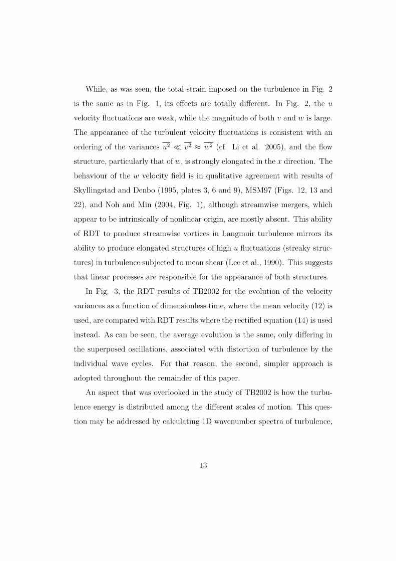
While, as was seen, the total strain imposed on the turbulence in Fig. 2

is the same as in Fig. 1, its effects are totally different. In Fig. 2, the u

velocity fluctuations are weak, while the magnitude of both v and w is large.

The appearance of the turbulent velocity fluctuations is consistent with an

ordering of the variances u2 ¿ v2 ≈ w2 (cf. Li et al. 2005), and the flow

structure, particularly that of w, is strongly elongated in the x direction. The

behaviour of the w velocity field is in qualitative agreement with results of

Skyllingstad and Denbo (1995, plates 3, 6 and 9), MSM97 (Figs. 12, 13 and

22), and Noh and Min (2004, Fig. 1), although streamwise mergers, which

appear to be intrinsically of nonlinear origin, are mostly absent. This ability

of RDT to produce streamwise vortices in Langmuir turbulence mirrors its

ability to produce elongated structures of high u fluctuations (streaky struc-

tures) in turbulence subjected to mean shear (Lee et al., 1990). This suggests

that linear processes are responsible for the appearance of both structures.

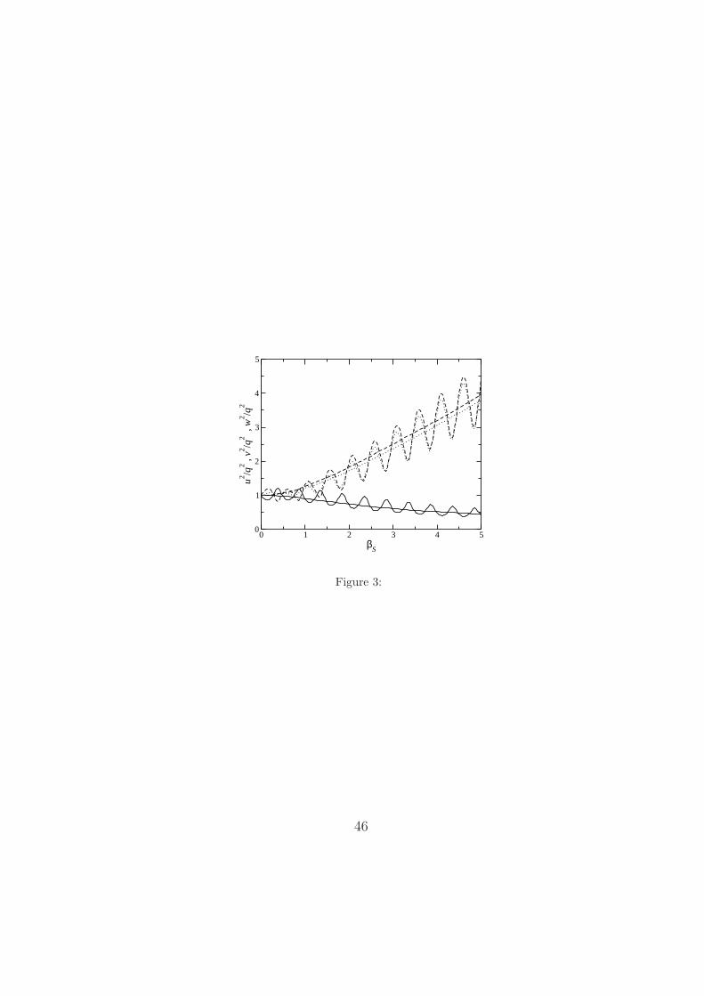
In Fig. 3, the RDT results of TB2002 for the evolution of the velocity

variances as a function of dimensionless time, where the mean velocity (12) is

used, are compared with RDT results where the rectified equation (14) is used

instead. As can be seen, the average evolution is the same, only differing in

the superposed oscillations, associated with distortion of turbulence by the

individual wave cycles. For that reason, the second, simpler approach is

adopted throughout the remainder of this paper.

An aspect that was overlooked in the study of TB2002 is how the turbu-

lence energy is distributed among the different scales of motion. This ques-

tion may be addressed by calculating 1D wavenumber spectra of turbulence,

13

which are defined as:

Sii(k1) =1

2π

∫ui(x, y, z)ui(x + r1, y, z)e−ik1r1dr1,

Sii(k2) =1

2π

∫ui(x, y, z)ui(x, y + r2, z)e−ik2r2dr2, (i = 1, 2, 3). (15)

Results from RDT presented in Fig. 4 show that, in shear turbulence

the energy of streamwise velocity fluctuations is increased at all scales in

the streamwise direction, while a peak develops at the integral length scale

in the spanwise direction. This is consistent with a ‘streaky structure’ of

u. Under a Stokes distortion, it is the vertical velocity fluctuations that are

increased: on a broad range of scales in the streamwise direction, and with

a peak in the spanwise direction. The main difference between shear and

wave-distorted turbulence in the spanwise fluctuations is that in the shear

turbulence the increase in v energy occurs primarily at small scales, while

in wave-distorted turbulence it occurs at all scales. These results essentially

confirm the interpretation of TB2002 based on the behaviour of the integral

length scales in shear and wave-distorted turbulence.

2.1.1. Blocking effect of the free surface

The Froude number of turbulence in the water is often sufficiently low that

the shape of the free surface bounding it above can be taken as specified and

fixed. This shape can either be flat (in the absence of surface waves, when the

distorting flow is a shear flow) or undulating (when the distorting flow is an

irrotational wave). The undulation associated with the wave may be treated

rigorously using curvilinear coordinates (TB2002). However, when the slope

of the distorting wave is small, these coordinates essentially coincide with

the Cartesian coordinates, and the air-water interface is also approximately

14

flat. In either of these two situations, the presence of the interface acts to

block the turbulence at the surface, so that the normal component of the

fluctuating vorticity is brought to zero at the interface.

The effect of blocking on isotropic turbulence is well-known (Hunt and

Graham, 1978; Hunt, 1984), resulting (in the RDT approximation) in an

amplification of the tangential velocity components of the turbulence at the

surface by a factor of 1.5, while the normal component tends to zero. For

a constant-shear flow, Fig. 5 shows that the blocking effect suppresses al-

most completely the streaky structures at the surface, making the u and v

field appear almost isotropic along x and y (cf. Lee and Hunt, 1989; Mann,

1994). This phenomenon, which is related to the generation of vorticity

in the blocking velocity correction (see Gartshore et al., 1983), would have

important consequences for surface transport if true in realistic conditions.

However, it is not supported by the DNS results of Tsai et al. (2005), where

streaky structures are seen to exist up to the surface. There are a number of

possible reasons for this disagreement. The assumption of initial irrotational-

ity of the blocking correction, or of a unique, constant, shear rate and length

scale, may not be appropriate, since in the DNS of Tsai et al. (2005) the

turbulence spreads from the free surface (through a surface stress) instead of

impacting on the interface from below, as implied by RDT.

In Fig. 6, the velocity field at the surface in turbulence distorted by a

surface wave is displayed. Here, both u and v are somewhat larger than in

the bulk of the fluid, but behave in qualitatively the same way, with v being

much larger than u, and showing a structure elongated in the x direction.

Obviously, this has important consequences for transport at the surface, as

15

will be seen next. By Hunt and Graham’s (1978) results (which hold in the

present case), the TKE must be the same in the bulk of the fluid and at the

surface. Thus, for turbulence distorted by a surface wave, v is amplified by

a factor larger than 1.5 (≈ 2) due to blocking, since u is relatively small in

the bulk of the fluid, but w must decay to zero at the surface, transferring

the whole of its energy to v in the process.

2.2. Surface transport of tracer particles

Fig. 7 shows the locations of 10000 tracer particles released randomly

at the surface for each of the flows considered. Fig. 7a displays the initial

particle positions. Figs. 7b and 7c display the particle spatial distributions

after an advection time qt/l = 1 (corresponding to one eddy turn-over time

of the initial turbulence), respectively for shear turbulence and turbulence

distorted by a wave. It can be seen that the tracer particles tend to ac-

cumulate in convergence zones of the surface velocity field, forming rows.

For turbulence distorted by a wave the particles accumulate in well-defined

rows clearly aligned in the streamwise direction. Given the nature and in-

tensity of v in this last case (see Fig. 6b), that behaviour is not surprising,

and is clearly in qualitative agreement with that observed in the LES of

Skyllingstad and Denbo (1995, plate 6), MSM97 (Fig. 10), McWilliams and

Sullivan (2001, Fig. 2) and Skyllingstad (2001, Figs. 2 and 3). It also re-

sembles the behaviour of surface tracers in the experimental studies of Faller

and Cartwright (1983), Nepf et al. (1995) and Melville et al. (1998). Taking

as an example for comparison Fig. 10 of MSM97, the time indicated in that

figure is t = 1440s. If the value of the integral length scale found later in

Section 3.4 is adopted, l = 7.5m, and the normalised shear stress is calcu-

16

lated using RDT for βS = 5 (the dimensionless time used to compute the

velocity field that advects the tracer in Fig. 7), this gives uw/q2 = −0.7.

Then q = 1.2u∗, and using the value u∗ = 6.1× 10−3m s−1 given by MSM97,

in Fig. 10 of MSM97 the advection time is qt/l = 1.4. Despite the many

differences between the two models, it is reassuring that this is at least of

the same order of magnitude as the advection time adopted in Fig. 7.

In the case of shear turbulence (Fig. 7b), the tracer rows are not so

well defined as in Fig. 7a, and have a more isotropic distribution, although

there is the hint of alignment in the streamwise direction. This is due to the

weakness of the associated advecting velocity field, mentioned above. The

DNS of shear turbulence near an interface computed by Tsai et al. (2005)

does have streaky structures at the surface and their tracer particles tend to

form much clearer rows in the streamwise direction than in Fig. 7b. However,

even if such streaks do exist, a flow whose dominant velocity fluctuation is

u with an elongated structure along x is, at least intuitively, less effective in

creating streamwise tracer rows than a flow with convergence zones along x in

the v velocity field. Fig. 8 shows schematically the different mechanisms for

the formation of tracer rows. While in shear flow these rows occur due to the

confluence of v at the entrance of the jet of high u, in a flow with streamwise

vortices the tracer rows are formed by the lines of strong convergence of the

v velocity field.

It has additionally been noted by Craik and Leibovich (1976), Leibovich

(1983), Cox and Leibovich (1993) and Thorpe (2004) that particles in these

streamwise rows of tracer travel in the direction of the mean flow faster

than the air-water interface itself, on average. In the context of turbulence,

17

this is easily explained by the existence of a shear stress. Since the tracer

accumulates above zones where the flow descends, in order to have a negative

shear stress near the surface, the u velocity perturbation must be positive

there. This argument, which also applies to shear turbulence, explains the

analogous behaviour of tracers in the DNS of Tsai et al. (2005). In the

case of wave-distorted turbulence, the tracer particles in our KST moved in

the direction of the wave propagation (or of the Stokes drift) with a velocity

exceeding the average interface velocity by 0.45q, a rather significant value.

These results illustrate the differences between turbulence in a shear flow

and turbulence distorted by a wave. A simple explanation of the differences

in terms of the dynamics of the vorticity is described in Appendix A. The

results of this section show that at least the qualitative aspects are captured

by the linear RDT and KST models. In the next two sections quantitative

comparisons are made between these models and LES of Langmuir turbu-

lence.

3. Scaling the large-scale structure of Langmuir turbulence

Polton and Belcher (2007) investigate the TKE budget of their LES of

Langmuir turbulence and show that in an upper Stokes layer, whose depth

scales on the depth of the Stokes drift, the dominant balance is between

production of TKE by the Stokes production, and dissipation (in the ab-

sence of wave breaking). Below this region turbulent transport carries TKE

downwards deep into the mixed layer. They then suggest a schematic where,

within the Stokes layer, the Stokes drift tilts and stretches vertical vortic-

ity into the horizontal. This generates convergence zones, which then leads

18

to downwelling jets that penetrate deep into the mixed layer (and trans-

port TKE through turbulent transport). We consider now whether or not

the linear RDT model can capture quantitatively the structure of Langmuir

turbulence computed in the LES, particularly in the Stokes layer.

Grant and Belcher (2009) have used the TKE budget to develop a scaling

for the resulting Langmuir turbulence, arguing that the appropriate velocity

scale is w∗L = (u2∗US0)

13 (see also Harcourt and D’Asaro, 2008) and the

appropriate length scale is h, the depth of the mixed layer. They show that

profiles of the turbulent velocity variances from a wide range of simulations,

when scaled by w2∗L and h, collapse onto single profiles. It is then sufficient to

consider results from a single simulation, and the focus here is on the shape

of the profiles of the velocity variances.

We focus on the LES run E/0.3 of Langmuir turbulence computed by

MSM97. Subsequent investigations (Li et al., 2005) have suggested that the

value of the turbulent Langmuir number used by MSM97 in this experiment is

fairly typical of ocean conditions. MSM97 consider a monochromatic wave of

amplitude aw = 0.8m and wavenumber kw = 2π/60rad m−1, so that the wave

slope is awkw = 0.084, and the angular frequency, obtained using the linear

dispersion relation of surface water waves, is σw = 1.0rad s−1. In addition,

they specified a surface wind stress with an associated friction velocity in the

water of u∗ = 6.1× 10−3m s−1, and a thermocline at h = 33m. These values

will be used here. For this simulation the Stokes layer occupies the region

0 < z/h < 0.4, a substantial fraction of the mixed layer (Grant and Belcher,

2009).

19

3.1. Deformation by shear and Stokes drift

Turbulence in the LES simulations of the wind-driven mixed layer is sub-

jected to straining from three sources: the presence of the air-sea interface;

the mean shear in the wind-driven current; and the Stokes drift associated

with the surface wave. Consider first the competing strains of the mean shear

and the Stokes drift, which can be measured by the parameter R, defined by

R =αS

α. (16)

This parameter gives the ratio of the production of TKE by the Stokes drift

and by shear, according to Equation (5.1) of MSM97. The variation of this

parameter is calculated next using results from the LES of MSM97.

Fig. 9a shows the variation with depth of the strain rate associated with

the Stokes drift of the wave (dashed line), derived from the parameters given

by MSM97. Also shown in Fig. 9a is the shear rate through the wind-driven

mixed layer derived from the mean velocity profiles computed by MSM97

for simulations with and without Stokes drift. Both cases are driven by a

surface wind stress, with an associated friction velocity (in the water) equal

to u∗ = 6.1 × 10−3m s−1. The case without Stokes drift, S/∞ (dotted line),

shows a shear rate that closely follows the form α = u∗/κz expected for a

logarithmic surface layer with the appropriate friction velocity. The shear

rate in the case with Stokes drift, E/0.3 (solid line), perhaps surprisingly,

also approximately follows the form expected for a logarithmic surface layer,

but this time with a much reduced friction velocity of 0.61× 10−3m s−1 (see

Fig. 9a). The reason is the following: once Langmuir turbulence is initiated,

mixing is promoted by the Langmuir circulations themselves reducing the

20

mean shear, perhaps augmented by the effects of the Coriolis force turning

the mean flow and reducing shear in the wave direction (see Polton et al.,

2005; Polton and Belcher, 2007). The assumption of a logarithmic mean

velocity profile, employed above, is an approximation primarily valid near

the surface, since, for example, Fig. 3a of MSM97 shows that the shear stress

in the x direction is not constant, but decreases with depth. However, as the

following scalings rely primarily on the flow parameters near the surface, say

for z < 0.4h, where the mean transport gradients are sufficiently strong, this

approximation is accurate enough for our purposes.

With these observations the parameter R for a single wave can be written

R =2(awkw)2σwe−2kwz

u∗s/κz, (17)

where u∗s is an effective friction velocity associated with the near-surface

shear. Fig. 9b shows the variation of R−1 with depth for run E/0.3, when

u∗s = 0.61 × 10−3m s−1 (solid line), together with values obtained from the

LES profiles (symbols). Also shown is the profile obtained using the full

friction velocity, u∗ = 6.1 × 10−3m s−1 (dotted line). When the mean shear

is correctly parameterised using u∗s, then R−1 ¿ 1 through most depths,

implying the strain by Stokes drift is greater than the strain by mean shear.

Towards the bottom of the wind-driven layer, 0.8 < z/h < 1, R < 1 but

at these depths strains by both Stokes drift and shear are weak, and the

turbulence is likely to be dominated by entrainment at the thermocline.

We conclude that in the presence of Stokes drift the turbulence is largely

distorted by Stokes drift because this situation is self-sustained by intense

vertical mixing. While turbulence can mix down momentum, it has no im-

pact on the Stokes drift gradient. The deformation by mean shear on the

21

turbulence can therefore be neglected.

3.2. Integral properties of Langmuir turbulence

The next step is to evaluate two integral properties of Langmuir turbu-

lence, which will then enable scaling arguments. Firstly, an estimate of the

integral length scale of the Langmuir turbulence computed by MSM97 is

evaluated using the approximation used in the K − ε turbulence closure (al-

though we note that this is only strictly valid for homogeneous and isotropic

turbulence), namely

l ∝ K32

ε⇒ l

h= c1

(K/u2∗)

32

εh/u3∗, (18)

where K is the TKE, ε is the rate of viscous dissipation and c1 is a dimen-

sionless constant of O(1). For homogeneous turbulence, the relation between

the dissipation rate ε, the turbulent root-mean square velocity q and the lon-

gitudinal length scale ε ∝ q3/l has been found by various authors (Pearson

et al., 2002; Kaneda et al., 2003) to have a proportionality constant approx-

imately between 0.5 and 1. In terms of (18), this would mean that c1 should

be between 0.27 and 0.54. Here we choose c1 = 0.387, which gives optimal

agreement between the RDT calculations and the LES data, as will be seen

below.

Figs. 4 and 5 of MSM97 present profiles of the normalised TKE, K/u2∗,

and of the normalised dissipation rate εh/u3∗. Fig. 10a shows a profile of

l/h, as defined in (18), derived from these LES data. It can be seen that the

integral length scale of the turbulence increases approximately linearly away

from the boundary. The dashed line in Fig. 10a represents a linear fit to the

22

LES data, namely

l/h = γ(z + dl)/h. (19)

The best fit yields a slope γ ≈ 0.35 and a value at the surface, akin to the

displacement height of a logarithmic layer, dl/h ≈ 0.42. A linear variation

in the integral length scale is a characteristic of either a shear-free turbulent

layer near an interface, which has γ ≈ 1 (Hunt 1984), or a constant-stress

logarithmic boundary layer, which has γ = κ ≈ 0.4, the von Karman constant

(Tennekes and Lumley, 1972). The latter value is surprisingly close to the

value of γ obtained here for the Langmuir turbulence.

We note that the value of the displacement height obtained from the LES

may be an artifact of the way the LES resolves the interface. Nevertheless

a non-zero value is probably realistic because the turbulence length scale is

determined by non-local factors. So it does not tend to zero at the surface,

because eddies of finite size approach the surface where they are blocked by

the air-water interface (Hunt, 1984). We note that the value of γ derived by

Grant and Belcher (2009) in their Fig. 6 is considerably larger that the value

found here. But they force their linear fit to intercept the origin, making

their value larger. A consistency check to our choice of c1 is that if the

integral length scale is everywhere smaller than l/h = 1, then l/h should

grow linearly until very close to z/h = 1, instead of tending to a constant

value, as in Grant and Belcher (2009). This is indeed confirmed by Fig. 10.

Secondly, the decorrelation time scale, or eddy turn-over time of the tur-

bulence, Te, is estimated by analogy with the integral length scale, namely

Te ∝ K

ε⇒ Teu∗

h=

K/u2∗

εh/u3∗. (20)

23

Note that in (20), and in contrast to (18), we have not included a constant of

proportionality, because the eddy turn-over time is generally not as precisely

defined in terms of the other quantities as the integral length scale, and also

because it is the form of its dependence on depth that will be of primary

interest for the RDT and KST calculations.

Fig. 10b shows the variation of u∗Te/h with depth computed from the

LES data of MSM97. The decorrelation time increases approximately linearly

with distance from the boundary, and can be fitted to

u∗Te

h= δ(z + dT )/h, (21)

with slope δ ≈ 1.0 and displacement height dT /h ≈ 0.08. This fit is shown

as the solid line in Fig. 10b. A linear increase in Te with distance from a

boundary is also a characteristic of shear-free turbulence near a boundary,

where δ ≈ 1, and a constant-stress logarithmic boundary layer, where δ = κ

(Tennekes and Lumley, 1972). The variation of the decorrelation time scale

in Langmuir turbulence is therefore similar to the variation in wall-bounded

shear-free turbulence.

In the simulations of MSM97 u∗ = 6.1 × 10−3m s−1, whence the decor-

relation time scale at the interface is Te0 = δdT /u∗ ≈ 430s, which is again

non-zero because Te receives contributions from eddies of finite size that reach

the surface from some distance below.

These two measures of the turbulence both increase away from the bound-

ary and so indicate the importance of the air-water interface in blocking

the turbulence. The behaviour of the integral length and time scales will

prove useful in estimating the nonlinear processes in the Langmuir turbu-

lence, which is done next.

24

3.3. Scaling the distortion of the turbulence

Consider now the velocity fluctuations in the Langmuir turbulence, q,

which scale on the friction velocity, u∗, (MSM97). The velocity associated

with the deformation of the turbulence is the Stokes drift, US = (awkw)2cwe−2kwz.

At the air-sea interface the ratio of these terms is

US/q ∼ (awkw)2cw/u∗. (22)

For the parameters of run E/0.3 in MSM97, this ratio is approximately equal

to 11—a large number. Similarly, the fluctuating strain rate associated with

the turbulence can be estimated to be q/l which scales as T−1e , whereas

the strain rate associated with the Stokes drift is αS. Using the expression

obtained from the LES in Section 3.2 for Te, the ratio of these terms is

αS

T−1e

∼ 2cw

u∗(awkw)2δkw(z + dT )e−2kwz. (23)

The maximum value of this ratio occurs at 2kw(z + dT ) = 1, when it takes

the valueαS

T−1e

∣∣∣max

∼ cw

u∗(awkw)2δ exp(2kwdT − 1), (24)

which, for case E/0.3 of MSM97, equals about 7—again a relatively large

number. Hence for this case at least the fluctuating turbulent velocity and

strain rates are much smaller than the velocity and strain rate associated

with the deformation due to the Stokes drift. This proves to be a key in

justifying a linearised RDT model for Langmuir turbulence in the Stokes

layer.

Finally, we note that the Froude number associated with the turbulent

motions is large, so that, as assumed in the LES, the turbulence does not

25

appreciably deform the interface, i.e.

aw À q2/g, (25)

where g is the acceleration of gravity. Hence the interface remains dominated

by the driving wave (cf. Brocchini and Peregrine, 2001).

3.4. Estimating the parameters of the RDT model

RDT is, mathematically, an initial-value problem and so requires specifi-

cation of the initial turbulence, and then specification of the integration time

of the distortion (or equivalently the total strain by the mean flow).

The initial turbulence is represented by the spectrum (10), which requires

specification of the integral length scale, l, and turbulent intensity, q. Here,

we will not need to specify q because velocity variances will be normalised

on q. Turbulence statistics will be shown here as a function of normalised

distance from the boundary, z/l, but the results of MSM97 are plotted as a

function of z/h. Hence we require a relation between l and h. Within the

RDT model the principal effect of the integral length scale is to determine

the depth of the blocking effect of the air-sea interface on the turbulence, and

hence we relate l and h here to match this blocking depth. The variation in

l with z obtained in Section 3.2 from the LES data shows that far from the

interface l < z, and hence the turbulence at these depths is unaffected by the

boundary, whereas near the interface l > z, and so the turbulence there is

directly affected by the blocking of the boundary. Hence in the RDT model

we use the value of the l obtained from the LES at the depth where l = z,

i.e. the intersection between the line y = l(z) in Fig. 10a and the line y = z.

The turbulence is then subjected to blocking over the correct distance from

26

the boundary. For the parameters of the MSM97 simulations, this procedure

yields l/h = 0.23, so that l = 7.5 m.

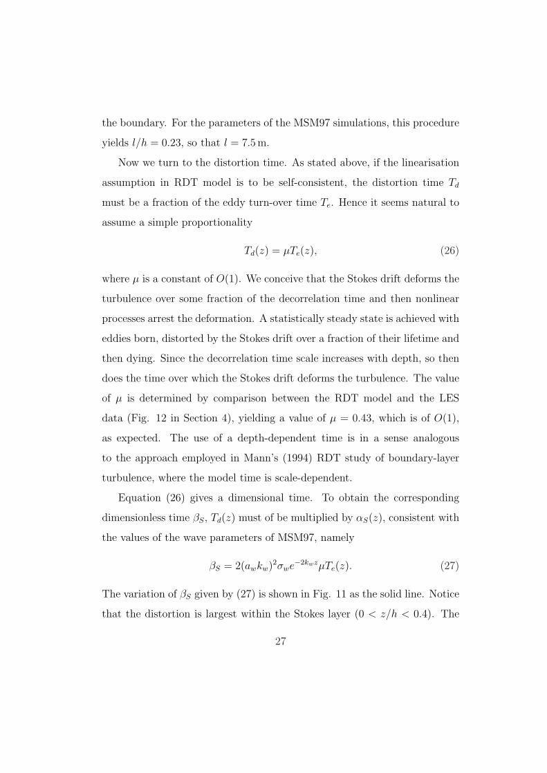
Now we turn to the distortion time. As stated above, if the linearisation

assumption in RDT model is to be self-consistent, the distortion time Td

must be a fraction of the eddy turn-over time Te. Hence it seems natural to

assume a simple proportionality

Td(z) = µTe(z), (26)

where µ is a constant of O(1). We conceive that the Stokes drift deforms the

turbulence over some fraction of the decorrelation time and then nonlinear

processes arrest the deformation. A statistically steady state is achieved with

eddies born, distorted by the Stokes drift over a fraction of their lifetime and

then dying. Since the decorrelation time scale increases with depth, so then

does the time over which the Stokes drift deforms the turbulence. The value

of µ is determined by comparison between the RDT model and the LES

data (Fig. 12 in Section 4), yielding a value of µ = 0.43, which is of O(1),

as expected. The use of a depth-dependent time is in a sense analogous

to the approach employed in Mann’s (1994) RDT study of boundary-layer

turbulence, where the model time is scale-dependent.

Equation (26) gives a dimensional time. To obtain the corresponding

dimensionless time βS, Td(z) must of be multiplied by αS(z), consistent with

the values of the wave parameters of MSM97, namely

βS = 2(awkw)2σwe−2kwzµTe(z). (27)

The variation of βS given by (27) is shown in Fig. 11 as the solid line. Notice

that the distortion is largest within the Stokes layer (0 < z/h < 0.4). The

27

dimensionless distortion time attains a maximum slightly above 3 near the

surface, but decays to zero with the Stokes drift as depth increases. This

is roughly consistent with the values of approximately 2 to 3 assumed in

numerous RDT studies (e.g. Townsend, 1970; Mann, 1994). Also shown in

Fig. 11 is the dimensionless time that would be obtained if the eddy turn-

over time had its surface value Te(z = 0) everywhere. In this case βS is

smaller, and exactly proportional to the Stokes drift strain rate.

A final comment is due. The LES of MSM97 use horizontal grid spac-

ings of ∆x = 3m and ∆x = 4.7m in experiments S/∞ and E/0.3, respec-

tively, and a vertical grid spacing of ∆z = 0.6m. This effectively limits the

wavenumbers that may be present in the LES turbulence spectrum. In par-

ticular, for the quoted cases, the dimensionless wavenumber in (10) is smaller

than k0l = 7.8 or k0l = 5.0 in the horizontal, respectively, while the vertical

wavenumber is smaller than k0l = 39.4. This anisotropy is not taken into

account in the spectral approach of RDT and KST so, since we are going

to focus primarily on Langmuir turbulence (experiment E/0.3) the spectrum

(10) is truncated at k0l = 5 in the calculations that follow, as was done in

Section 2 without the present justifications.

4. Comparison between RDT and LES results

Results calculated with RDT and KST using the previously estimated

parameters are now compared with those computed by MSM97 in their LES.

Firstly statistics of the distorted turbulence are calculated to show how the

profiles are shaped by the combination of Stokes drift, blocking by the inter-

face, and variation of the turbulence scale with distance from the interface,

28

modelled here by allowing Te to vary with depth. Secondly, a realisation of

the turbulent flow similar to that presented in Section 2, but for the specific

conditions considered in MSM97 is calculated using KST.

4.1. Profiles of the turbulent velocity variances

Fig. 12a shows the turbulent velocity variances normalised on TKE,

u2i /

23K, calculated from RDT and comparisons with the LES data presented

in Fig. 6 of MSM97 for run E/0.3. Note that RDT is an initial-value problem,

so it is appropriate to compare the ratios of the turbulence intensities, but

not their actual values, since these are dependent on the initial conditions.

The RDT results in Fig. 12a agree remarkably well with the LES data,

particularly in the Stokes layer 0 < z/h < 0.4. Deep in the mixed layer, for

z/h larger than about 0.7 the variances are approximately isotropic (when

the normalised variance is 1 by definition). (w2/23K is slightly smaller—

probably a consequence of the thermocline at z/h = 1 in the LES.) Nearer

the surface, in 0.2 < z/h < 0.7, the streamwise variance, u2/23K, decreases,

while v2/23K and w2/2

3K both increase towards the interface. By z/h = 0.2,

v2/23K and w2/2

3K are considerably larger than u2/2

3K. This behaviour

is consistent with the generation of streamwise vortices by the tilting and

stretching of vertical vorticity into the streamwise direction by the Stokes

drift (TB2002). In the region 0 < z/h < 0.2, v2/23K and u2/2

3K increase

towards the interface, while w2/23K is forced to decrease to zero. This region

corresponds to z/l < 1 and so is caused by the blocking effect of the interface

on the turbulence distorted by the Stokes drift.

Consider now how different parts of the RDT solution give different parts

of the response. Fig. 12b presents profiles of the turbulent velocity variances

29

for the same conditions as in Fig. 12a, except that the deformation is allowed

for the same time through the whole depth of the layer (dotted line in Fig.

11). Hence the model is truncated after a dimensionless distortion time βS

corresponding to the eddy turn-over time valid at the surface through all

depths. Although the RDT values near the surface are close to the data, the

anisotropy due to distortion by the wave motion decays too fast away from

the interface, because the distortion by the Stokes drift at large depths is not

allowed to act for a sufficiently long interval of time.

If, on the other hand, the Stokes drift distortion is neglected altogether

and only the blocking effect of the interface is taken into account then RDT

yields the results shown in Fig. 12c. Both u2/23K and v2/2

3K now increase

towards the interface (by the same amount since the deformation is now

isotropic in the horizontal) and w2/23K decreases by the blocking mechanism

towards the interface. But the amplification of v2/23K and w2/2

3K and the

attenuation of u2/23K farther from the interface is not produced.

The agreement between the RDT model and the LES data is better in

the upper layer, 0 < z/h < 0.4, which corresponds to the Stokes layer. This

is consistent with the findings of Polton and Belcher (2007) and Grant and

Belcher (2009) that within this upper Stokes layer the dominant balance

in the TKE budget is between Stokes production and dissipation, whereas

deeper in the layer turbulent transport (which is nonlinear and so not cap-

tured in RDT) is a dominant term in the TKE budget. Finally, we recall

that deformation by shear would produce a completely different structure

with u2 > v2 > w2, as was shown earlier in this paper, and also in TB2002.

We conclude that linear processes to a large extent shape the anisotropy of

30

the turbulence.

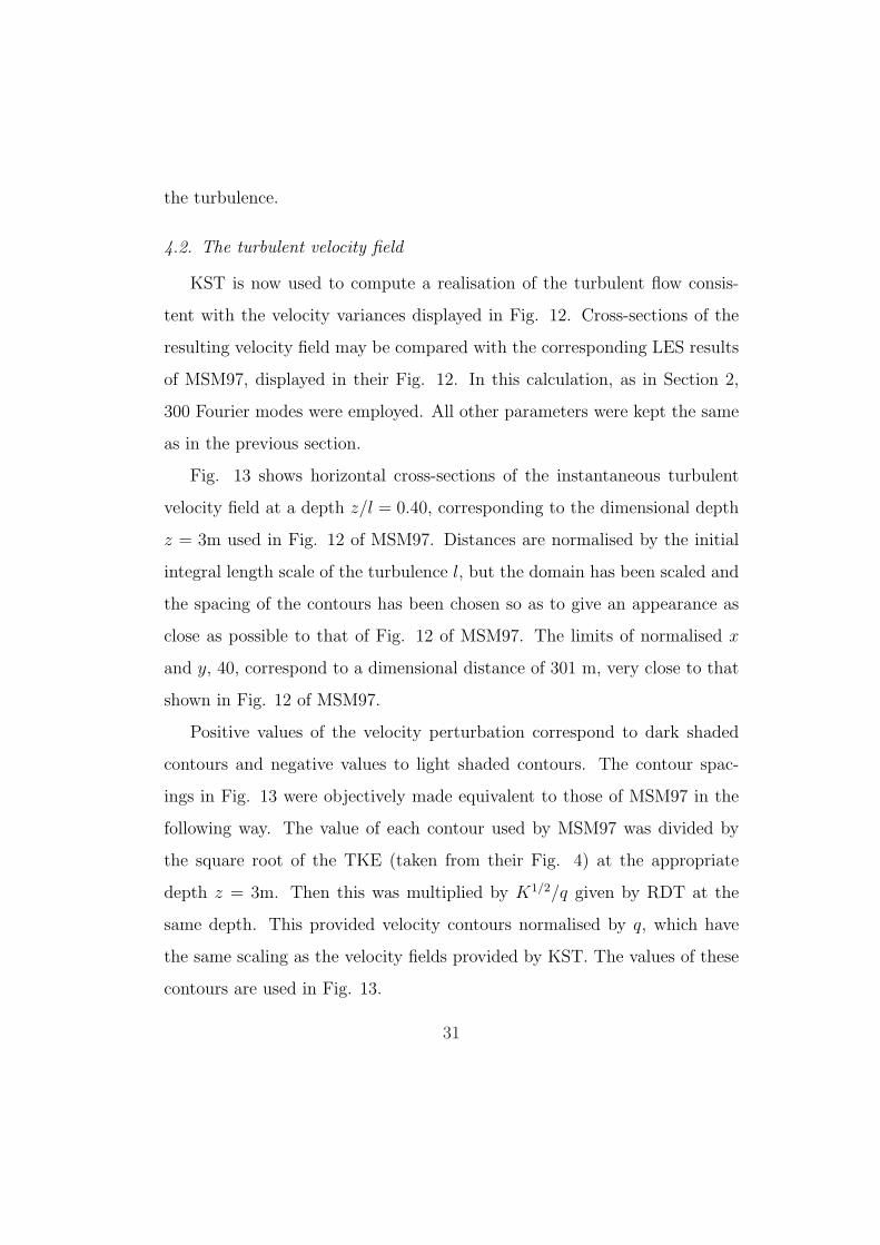
4.2. The turbulent velocity field

KST is now used to compute a realisation of the turbulent flow consis-

tent with the velocity variances displayed in Fig. 12. Cross-sections of the

resulting velocity field may be compared with the corresponding LES results

of MSM97, displayed in their Fig. 12. In this calculation, as in Section 2,

300 Fourier modes were employed. All other parameters were kept the same

as in the previous section.

Fig. 13 shows horizontal cross-sections of the instantaneous turbulent

velocity field at a depth z/l = 0.40, corresponding to the dimensional depth

z = 3m used in Fig. 12 of MSM97. Distances are normalised by the initial

integral length scale of the turbulence l, but the domain has been scaled and

the spacing of the contours has been chosen so as to give an appearance as

close as possible to that of Fig. 12 of MSM97. The limits of normalised x

and y, 40, correspond to a dimensional distance of 301 m, very close to that

shown in Fig. 12 of MSM97.

Positive values of the velocity perturbation correspond to dark shaded

contours and negative values to light shaded contours. The contour spac-

ings in Fig. 13 were objectively made equivalent to those of MSM97 in the

following way. The value of each contour used by MSM97 was divided by

the square root of the TKE (taken from their Fig. 4) at the appropriate

depth z = 3m. Then this was multiplied by K1/2/q given by RDT at the

same depth. This provided velocity contours normalised by q, which have

the same scaling as the velocity fields provided by KST. The values of these

contours are used in Fig. 13.

31

It can be seen that the u velocity fluctuations are relatively weak and

decorrelate over a large distance. The v and the w velocity fluctuations are

more intense and the spatial structure of the w velocity fluctuations reveals

a compression in the y direction and an elongation in the x direction. As

noted in Fig. 2, this spatial structure is the signature of intense and elon-

gated streamwise vortices akin to Langmuir circulations. There is a striking

similarity between Fig. 13 and Fig. 12 of MSM97, especially for the w fluctu-

ations, but also somewhat for the u field. The agreement of v is a little worse,

with the present calculations not producing sufficient streamwise elongation.

Anyway, it is surprising that KST, with its linearising assumptions, is able

to reproduce so many features of this fully nonlinear turbulent flow.

5. Conclusions

The linearised dynamics encapsulated in rapid distortion theory and kine-

matic simulation of turbulence were used to understand differences between

shear turbulence and Langmuir turbulence in the ocean mixed layer. In the

case of turbulence distorted by a mean shear, there is a cancellation in the

linearised dynamics between distortion of the turbulent vorticity by the mean

flow and distortion of the mean vorticity by the turbulent flow. Consequently

streamwise vorticity is not produced by mean shear. Instead the main ef-

fect is a generation of vertical vorticity that leads to the streaky structures

that are widely observed in shear flows. The velocity variances are then or-

dered as u2 > v2 > w2. In the case of turbulence distorted by Stokes drift

the cancellation no longer occurs, because the Stokes drift does not have

mean vorticity. The result is that vertical vorticity is tilted into the hori-

32

zontal to form streamwise vortices. The velocity variances are then ordered

as u2 ¿ v2 ≈ w2. These qualitative results suggested that the important

processes in Langmuir turbulence are controlled by linear dynamics.

These qualitative findings motivated a quantitative model for the turbu-

lence velocity variances computed in Langmuir turbulence based on linearised

RDT. Since Grant and Belcher (2009) have demonstrated that, when ap-

propriately scaled, the profiles of turbulence variances collapse onto a single

profile, it is sufficient for the RDT model to be compared with a single case of

the LES model. Consequently, we used the data from an LES run by MSM97

to demonstrate that the formal approximations made in the linearised RDT

model are satisfied in the LES. In particular the scalings demonstrate that

in Langmuir turbulence the Stokes drift is a more potent force for distortion

of turbulence than is either the mean shear or the turbulent velocity fluc-

tuations themselves. The reason presumably is that the enhanced vertical

mixing by the Langmuir circulation mixes out the mean shear, but leaves

the Stokes drift unaffected. Consequently we developed here a quantitative

linearised RDT model for Langmuir turbulence that includes (i) deformation

of turbulent vorticity by the Stokes drift, (ii) blocking of vertical velocity

fluctuations by the air–sea interface and (iii) a distortion time that increases

with depth reflecting the increase of the eddy decorrelation time with depth

found in LES data.

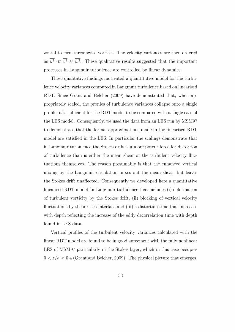
Vertical profiles of the turbulent velocity variances calculated with the

linear RDT model are found to be in good agreement with the fully nonlinear

LES of MSM97 particularly in the Stokes layer, which in this case occupies

0 < z/h < 0.4 (Grant and Belcher, 2009). The physical picture that emerges,

33

at least in the LES, is as follows. Early in the life cycle of a Langmuir eddy

initial turbulent disturbances of vertical vorticity are amplified algebraically

by the Stokes drift into elongated streamwise vortices, the Langmuir eddies.

The turbulence is thus in a near two-component state, with u2 suppressed

and v2 ≈ w2. Near the surface, over a depth of order the integral length scale

of the turbulence, the vertical velocity is brought to zero, by blocking of the

air–sea interface. Since, the turbulence is nearly two-component the energy

has to go into the spanwise fluctuations, enhancing v2 at the interface. After

a time of order half the eddy decorrelation time the nonlinear processes,

such as distortion by the strain field of the surrounding eddies, arrest the

deformation and the Langmuir eddy decays. The Langmuir turbulence then

consists of a statistically steady state of such Langmuir eddies.

The RDT model therefore throws light upon the dynamics within the

Stokes layer of the ocean mixed layer, where the Stokes drift operates and

the production of TKE by Stokes production balances dissipation. Deeper

into the mixed layer turbulent transport of TKE balances dissipation, which

Polton and Belcher (2007) suggest is mediated by downwelling jets originat-

ing in the convergence zones within the Stokes layer. Although turbulent

transport is a nonlinear process, and therefore not captured in the RDT

model, the flux of TKE comes from the Stokes layer, which is well mod-

elled by RDT, and so it may well be that RDT estimates can be used to

parameterise this flux.

34

Acknowledgement

We are grateful for the constructive comments of two anonymous referees.

M. A. C. T. acknowledges the financial support of Fundacao para a Ciencia

e Tecnologia (FCT) under Project AWARE/PTDC-ATM/65125/2006.

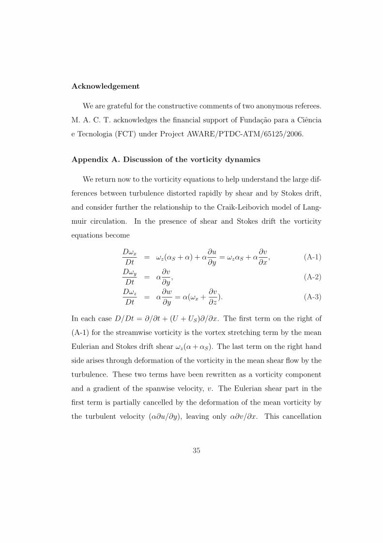
Appendix A. Discussion of the vorticity dynamics

We return now to the vorticity equations to help understand the large dif-

ferences between turbulence distorted rapidly by shear and by Stokes drift,

and consider further the relationship to the Craik-Leibovich model of Lang-

muir circulation. In the presence of shear and Stokes drift the vorticity

equations become

Dωx

Dt= ωz(αS + α) + α

∂u

∂y= ωzαS + α

∂v

∂x, (A-1)

Dωy

Dt= α

∂v

∂y, (A-2)

Dωz

Dt= α

∂w

∂y= α(ωx +

∂v

∂z). (A-3)

In each case D/Dt = ∂/∂t + (U + US)∂/∂x. The first term on the right of

(A-1) for the streamwise vorticity is the vortex stretching term by the mean

Eulerian and Stokes drift shear ωz(α + αS). The last term on the right hand

side arises through deformation of the vorticity in the mean shear flow by the

turbulence. These two terms have been rewritten as a vorticity component

and a gradient of the spanwise velocity, v. The Eulerian shear part in the

first term is partially cancelled by the deformation of the mean vorticity by

the turbulent velocity (α∂u/∂y), leaving only α∂v/∂x. This cancellation

35

is the key aspect determining differences between shear and wave-distorted

turbulence (see also Fig. 15 of TB2002).

The vertical vorticity equation has a vortex stretching term resulting from

interaction of the turbulent velocity with the mean vorticity (α∂w/∂y). This

term is written as a sum of αωx and α∂v/∂z. The equation for ωy also

contains a term involving v, corresponding physically to stretching of the

mean spanwise vorticity by the turbulence.

From energy arguments, it can be shown that the variance of v is not

directly affected by energy production terms, but only by the redistribution

of the turbulence energy through the pressure. For that reason, all terms

involving v in (A-1)-(A-3) will not be considered in the following schematic

argument (they are retained in the full RDT calculations).

Equations (A-1)-(A-3) then show in a simplified way how the coupling

between the components of the vorticity is different in the three cases of

distortion by mean shear, Stokes drift and both mean shear and Stokes drift.

When the deformation is by mean shear only, the essential process acting

is the conversion of streamwise into vertical vorticity by the term αωx in the

ωz budget. This causes the dominance of the u and v velocity fluctuations in

shear turbulence. (Although this is not the whole story. If only ωz increased,

u and v should tend to have the same intensity in highly sheared turbulence,

which is known not to be the case (e.g. Lee et al., 1990). In fact, other

components of vorticity, generated by the processes associated with the v-

terms, must play a role in producing the approximately one-dimensional

structure that highly sheared turbulence has).

When deformation is by the Stokes drift only, the situation is considerably

36

simpler: ωy and ωz do not vary much, but ωx strongly increases due to tilting

and stretching of ωz by the Stokes drift shear, as pointed out by TB2002.

This situation, which corresponds to the dominance of v and w velocity

fluctuations of approximately similar intensity, is consistent with streamwise

rolls, or Langmuir circulations.

Finally, when both shear and the Stokes drift are present, if the terms

involving v are again ignored, (A-1)-(A-3) give a coupled differential equation

set for ωx and ωz, from which separate equations for each of these quantities

can be isolated. It then results that both ωx and ωz grow exponentially

in time, with a growth rate proportional to (ααS)1/2. This growth rate is

typical of Langmuir circulations in a neutrally stratified ocean, as shown by

Leibovich (1977).

References

Batchelor, G. K., Proudman, I., 1954. The effect of rapid distortion of a

fluid in turbulent motion. Quarterly Journal of Mechanics and Applied

Mathematics 7, 83–103.

Brocchini, M., Peregrine, D. H., 2001. The dynamics of strong turbulence at

free surfaces. Part 1. Description. Journal of Fluid Mechanics 449, 225–254.

Cox, S. M., Leibovich, S., 1993. Langmuir circulations in a surface layer

bounded by a strong thermocline. Journal of Physical Oceanography 23,

1330–1345.

Craik, A. D. D., 1977. The generation of Langmuir circulations by an insta-

bility mechanism. Journal of Fluid Mechanics 81, 209–223.

37

Craik, A. D. D., Leibovich, S., 1976. A rational model for Langmuir circula-

tions. Journal of Fluid Mechanics 73, 401–426.

D’Asaro, E., 2001. Turbulent vertical kinetic energy in the ocean mixed layer.

Journal of Physical Oceanography 31, 3530–3537.

Dubrulle, B., Laval, J.-P., Nazarenko, S., Zaboronski, O., 2004. A model

for rapid stochastic distortions of small-scale turbulence. Journal of Fluid

Mechanics 520, 1–21.

Durbin, P. A., 1981. Distorted turbulence in axisymmetric flow. Quarterly

Journal of Mechanics and Applied Mathematics 34, 489–500.

Faller, A. J., Auer, S. J., 1988. The roles of Langmuir circulations in the

dispersion of surface tracers. Journal of Physical Oceanography 18, 1108–

1123.

Faller, A. J., Cartwright, R. W., 1983. Laboratory studies of Langmuir cir-

culations. Journal of Physical Oceanography 13, 329–340.

Fung, J. C. H., Hunt, J. C. R., Malik, N. A., Perkins, R. J., 1992. Kinematic

simulation of homogeneous turbulence by unsteady random Fourier modes.

Journal of Fluid Mechanics 236, 281–318.

Garrett, C., 1996. Processes in the surface mixed layer of the ocean. Dynamics

of Atmospheres and Oceans 23, 19–34.

Gartshore, I. S., Durbin, P. A., Hunt, J. C. R., 1983. The production of

turbulent stress in a shear flow by irrotational fluctuations. Journal of

Fluid Mechanics 137, 307–329.

38

Grant, A. L. M., Belcher, S. E., 2009. Characteristics of Langmuir turbulence

in the ocean mixed layer. Journal of Physical Oceanography, in press.

Harcourt, R. R., D’Asaro, E. A., 2008. Large-eddy simulation of Langmuir

turbulence in pure wind seas. Journal of Physical Oceanography 38, 1542–

1562.

Hunt, J. C. R., 1973. A theory of flow round two-dimensional bluff bodies.

Journal of Fluid Mechanics 61, 625–706.

Hunt, J. C. R., 1984. Turbulence structure in thermal convection and shear-

free boundary layers. Journal of Fluid Mechanics 138, 161–184.

Hunt, J. C. R., Graham, J. M. R., 1978. Free stream turbulence near plane

boundaries. Journal of Fluid Mechanics 84, 209–235.

Hunt, J. C. R., Kawai, H., Ramsey, S. R., Pedrizetti, G., Perkins, R. J., 1990.

A review of velocity and pressure fluctuations in turbulent flows around

bluff bodies. Journal of Wind Engineering and Industrial Aerodynamics

35, 49–85.

Kaneda, Y., Ishihara, T., Yokokawa, M., Itakura, K., Uno, A, 2003. Energy

dissipation rate and energy spectrum in high resolution direct numerical

simulations of turbulence in a periodic box. Physics of Fluids 15, L21–L24.

Kantha, L. H., Clayson, C. A., 2004. On the effect of surface gravity waves

on mixing in the oceanic mixed layer. Ocean Modelling 6, 101–124.

Lee, M. J., Hunt, J. C. R., 1989. The structure of sheared turbulence near

a plane boundary, in: Durst, F. et al. (Eds.), Seventh Symposium on

39

Turbulent Shear Flows, Stanford University, Stanford, California, USA,

Aug. 21–23 1989, pp. 8.1.1–8.1.6.

Lee, M. J., Kim, J., Moin, P., 1990. Structure of turbulence at high shear

rate. Journal of Fluid Mechanics 216, 561–583.

Leibovich, S., 1977. On the evolution of the system of wind drift currents and

Langmuir circulations in the ocean. Part 1. Theory and averaged current.

Journal of Fluid Mechanics 79, 715–743.

Leibovich, S., 1980. On wave-current interaction theories of Langmuir circu-

lations. Journal of Fluid Mechanics 99, 715-724.

Leibovich, S., 1983. The form and dynamics of Langmuir circulations. Annual

Review of Fluid Mechanics 15, 391–427.

Leibovich, S., Paolucci, S., 1981. The instability of the ocean to Langmuir

circulations. Journal of Fluid Mechanics 102, 141–167.

Leibovich, S., Radhakrishnan, K., 1977. On the evolution of the system of

wind drift currents and Langmuir circulations in the ocean. Part 2: Struc-

ture of the Langmuir vortices. Journal of Fluid Mechanics 80, 481–507.

Li, M., Garrett, C., Skyllingstad, E., 2005. A regime diagram for classifying

turbulent large eddies in the upper ocean. Deep-sea Research 52, 259–278.

Magnaudet, J., 2003. High-Reynolds number turbulence in a shear-free

boundary layer: revisiting the Hunt-Graham theory. Journal of Fluid Me-

chanics 484, 167-196.

40

Mann, J., 1994. The spatial structure of neutral atmospheric surface-layer

turbulence. Journal of Fluid Mechanics 273, 141–168.

McWilliams, J. C., Sullivan, P. P., 2001. Vertical mixing by Langmuir circu-

lations. Spill Science Technology 6, 225–237.

McWilliams, J. C., Sullivan, P. P., Moeng, C.-H., 1997. Langmuir turbulence

in the ocean. Journal of Fluid Mechanics 334, 1–30.

Melville, W. K., Shear, R., Veron, F., 1998. Laboratory measurements of

the generation and evolution of Langmuir circulations. Journal of Fluid

Mechanics 364, 31–58.

Nepf, H. M., Monismith, S. G., 1991. Experimental study of wave-induced

longitudinal vortices. Journal of Hydraulic Engineering 117, 1639–1649.

Nepf, H. M., Cowen, E. A., Kimmel, S. J., Monismith, S. J., 1995. Longi-

tudinal vortices beneath breaking waves. Journal of Geophysical Research

100, 16211–16221.

Noh, Y. and Min, H. S., 2004. Large eddy simulation of the ocean mixed

layer: the effects of wave breaking and Langmuir circulation. Journal of

Physical Oceanography 34, 720–735.

Pearson, B. R., Krogstad, P.-A., van de Water, W., 2002. Measurements of

the turbulent energy dissipation rate. Physics of Fluids 14, 1288–1290.

Perkins, R. J., Carruthers, D. J., Drayton, M. J., Hunt, J. C. R., 1990.

Turbulence and diffusion at density interfaces, in: Hewitt, G. F., Mayinger,

41

F., Riznic, J. R. (Eds.), Phase-interface phenomena in multiphase flow,

Hemisphere, pp. 21–30.

Pluddemann, A. J., Smith, J. A., Farmer, D. M., Weller, R. A., Crawford, W.

R., Pinkel, R., Vagle, S., Gnanadesikan, A., 1996. Structure and variabil-

ity of Langmuir circulation during the Surface Waves Processes Program.

Journal of Geophysical Research 101, 3525–3543.

Polton, J. A., Lewis, D. M., Belcher, S. E., 2005. The role of wave-induced

Coriolis-Stokes forcing on the wind-driven mixed layer. Journal of Physical

Oceanography 35, 444–457.

Polton, J. A., Belcher, S. E., 2007. Langmuir turbulence and deeply pene-

trating jets in an unstratified mixed layer. Journal of Geophysical Research

112, C09020.

Skyllingstad, E. D., 2001. Scales of Langmuir circulation generated using a

large-eddy simulation model. Spill Science Technology 6, 239–246.

Skyllingstad, E. D., Dembo, D. W., 1995. An ocean large-eddy simulation of

Langmuir circulations and convection in the surface mixed layer. Journal

of Geophysical Research 100, 8501–8522.

Smith, J. A., 1998. Evolution of Langmuir circulation during a storm. Journal

of Geophysical Research 103, 12649–12668.

Teixeira, M. A. C., Belcher, S. E., 2000. Dissipation of shear-free turbulence

near boundaries. Journal of Fluid Mechanics 422, 167–191.

42

Teixeira, M. A. C., Belcher, S. E., 2002. On the distortion of turbulence by

a progressive surface wave. Journal of Fluid Mechanics 458, 229–267.

Teixeira, M. A. C., Belcher, S. E., 2006. On the initiation of surface waves

by turbulent shear flow. Dynamics of Atmospheres and Oceans 41, 1–27.

Tennekes, H., Lumley, J. L., 1972. A first course in turbulence, the MIT

Press, Cambridge, Massachusetts, and London, England.

Thorpe, S. A., 2001. Langmuir circulation and the dispersion of oil spills in

shallow seas. Spill Science Technology 6, 213–223.

Thorpe, S. A., 2004. Langmuir circulation. Annual Review of Fluid Mechan-

ics 36, 55–77.

Townsend, A. A., 1970. Entrainment and the structure of turbulent flow.

Journal of Fluid Mechanics 41, 13–46.

Tsai, W.-T., Chen, S.-M., Moeng, C.-H., 2005. A numerical study on the

evolution and structure of a stress-driven free-surface turbulent shear flow.

Journal of Fluid Mechanics 545, 163–192.

Turfus, C., Hunt, J. C. R., 1987. A stochastic analysis of the displacements

of fluid elements in inhomogeneous turbulence using Kraichnan’s method

of random modes, in Comte-Bellot, G., Mathieu, J. (Eds.), Advances in

Turbulence. Springer-Verlag, Berlin, pp. 191–203.

43

0 2 4 6 8 10 12 14 16 18 20

x/l

0

2

4

6

8

10

12

14

16

18

20

y/l

(a)

0 2 4 6 8 10 12 14 16 18 20

x/l

0

2

4

6

8

10

12

14

16

18

20

y/l

(b)

0 2 4 6 8 10 12 14 16 18 20

x/l

0

2

4

6

8

10

12

14

16

18

20

y/l

(c)

Figure 1:

44

0 2 4 6 8 10 12 14 16 18 20

x/l

0

2

4

6

8

10

12

14

16

18

20

y/l

(a)

0 2 4 6 8 10 12 14 16 18 20

x/l

0

2

4

6

8

10

12

14

16

18

20

y/l

(b)

0 2 4 6 8 10 12 14 16 18 20

x/l

0

2

4

6

8

10

12

14

16

18

20

y/l

(c)

Figure 2:

45

0 1 2 3 4 5β

S

0

1

2

3

4

5

u2 /q2 ,

v2 /q2 ,

w2 /q

2

Figure 3:

46

0.01 0.1 1 10 1000.01

0.1

1

10 (a)

πSuu

(k1)

/(q2 l)

k1l

0.01 0.1 1 10 1000.01

0.1

1

10 (b)

πSvv

(k1)

/(q2 l)

k1l

0.01 0.1 1 10 1000.01

0.1

1

10 (c)

πSw

w(k

1)/(

q2 l)

k1l

0.01 0.1 1 10 1000.01

0.1

1

10 (d)

πS

uu(k

2)/(

q2 l)

k2l

0.01 0.1 1 10 1000.01

0.1

1

10 (e)

πSvv

(k2)

/(q2 l)

k2l

0.01 0.1 1 10 1000.01

0.1

1

10 (f)

πSw

w(k

2)/(

q2 l)

k2l

Figure 4:

47

0 2 4 6 8 10 12 14 16 18 20

x/l

0

2

4

6

8

10

12

14

16

18

20

y/l

(a)

0 2 4 6 8 10 12 14 16 18 20

x/l

0

2

4

6

8

10

12

14

16

18

20

y/l

(b)

Figure 5:

48

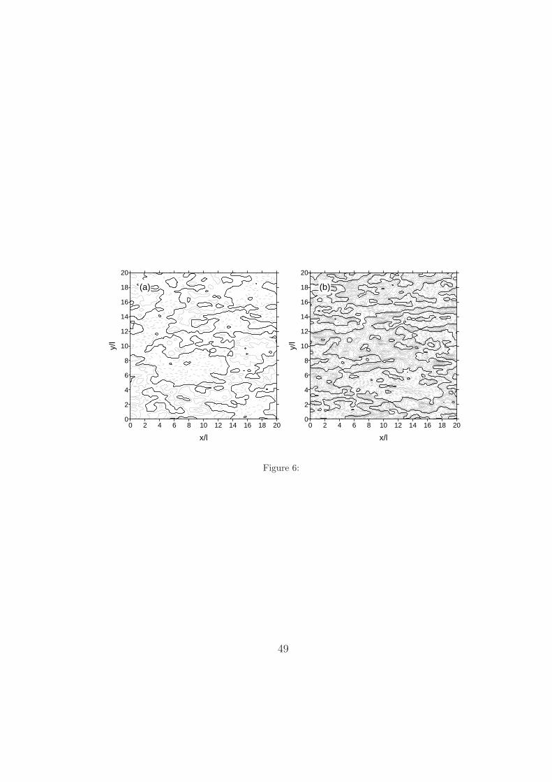
0 2 4 6 8 10 12 14 16 18 20

x/l

0

2

4

6

8

10

12

14

16

18

20

y/l

(a)

0 2 4 6 8 10 12 14 16 18 20

x/l

0

2

4

6

8

10

12

14

16

18

20

y/l

(b)

Figure 6:

49

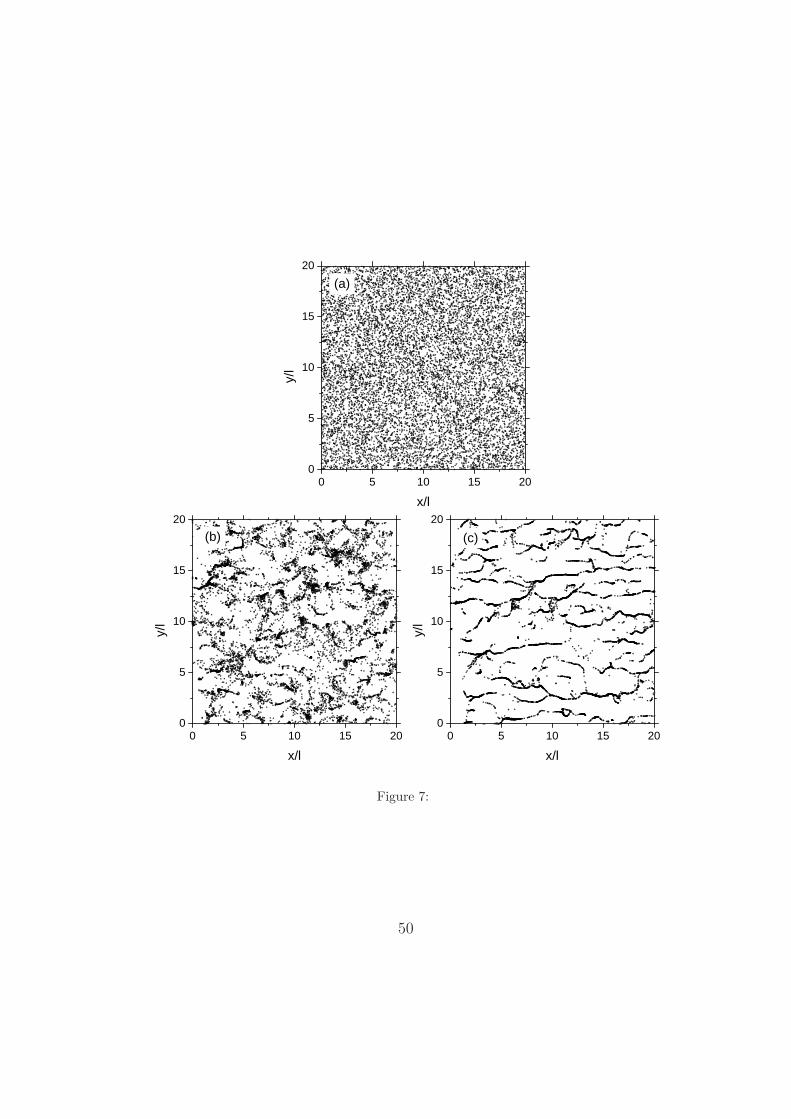
0 5 10 15 200

5

10

15

20

(a)

y/l

x/l

0 5 10 15 200

5

10

15

20

(b)

y/l

x/l

0 5 10 15 200

5

10

15

20

(c)

y/l

x/l

Figure 7:

50

WaveShear

Figure 8:

51

0.0 0.2 0.4 0.6 0.8 1.0z/h

-0.01

0

0.01

0.02

α,α S(s

-1)

(a)

0.0 0.2 0.4 0.6 0.8 1.0z/h

-0.5

0

0.5

1

1.5

2

R-1

(b)

Figure 9:

52

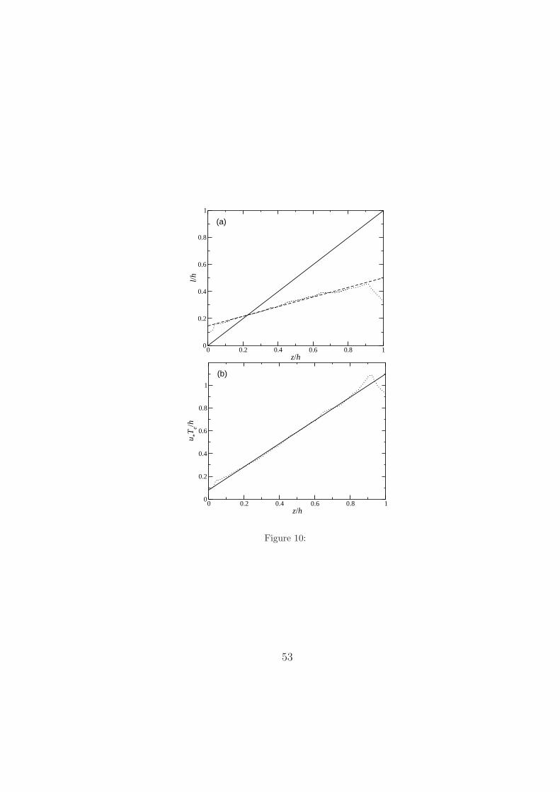
0 0.2 0.4 0.6 0.8 1z/h

0

0.2

0.4

0.6

0.8

1

l/h

(a)

0 0.2 0.4 0.6 0.8 1z/h

0

0.2

0.4

0.6

0.8

1

u *Te/h

(b)

Figure 10:

53

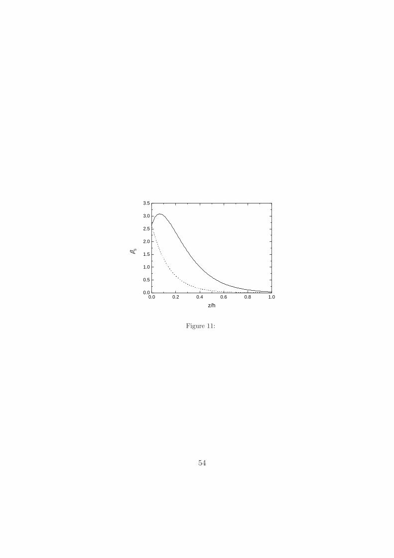
0.0 0.2 0.4 0.6 0.8 1.00.0

0.5

1.0

1.5

2.0

2.5

3.0

3.5

β S

z/h

Figure 11:

54

0 0.5 1 1.5 2 2.5 3 3.5z/l

0

0.5

1

1.5

2

2.5

u2 /(2/

3K),

v2 /(

2/3K

), w

2 /(2/

3K)

0 0.2 0.4 0.6 0.8z/h

0

0.5

1

1.5

2

2.5

(a)

0 0.5 1 1.5 2 2.5 3 3.5z/l

0

0.5

1

1.5

2

2.5

u2 /(2/

3K),

v2 /(

2/3K

), w

2 /(2/

3K)

0 0.2 0.4 0.6 0.8z/h

0

0.5

1

1.5

2

2.5

(b)

0 0.5 1 1.5 2 2.5 3 3.5z/l

0

0.5

1

1.5

2

2.50 0.2 0.4 0.6 0.8

z/h

0

0.5

1

1.5

2

2.5

u2 /(2/

3K),

v2 /(

2/3K

), w

2 /(2/

3K)

(c)

Figure 12:

55

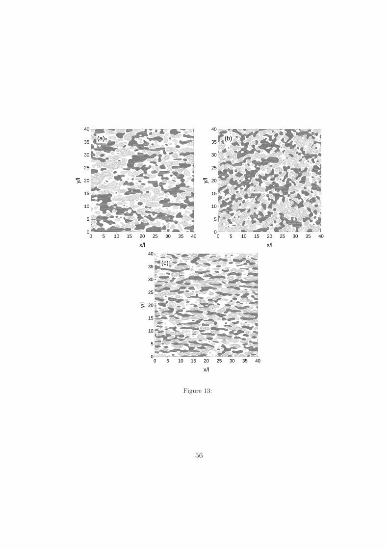
0 5 10 15 20 25 30 35 40

x/l

0

5

10

15

20

25

30

35

40

y/l

(a)

0 5 10 15 20 25 30 35 40

x/l

0

5

10

15

20

25

30

35

40

y/l

(b)

0 5 10 15 20 25 30 35 40

x/l

0

5

10

15

20

25

30

35

40

y/l

(c)

Figure 13:

56

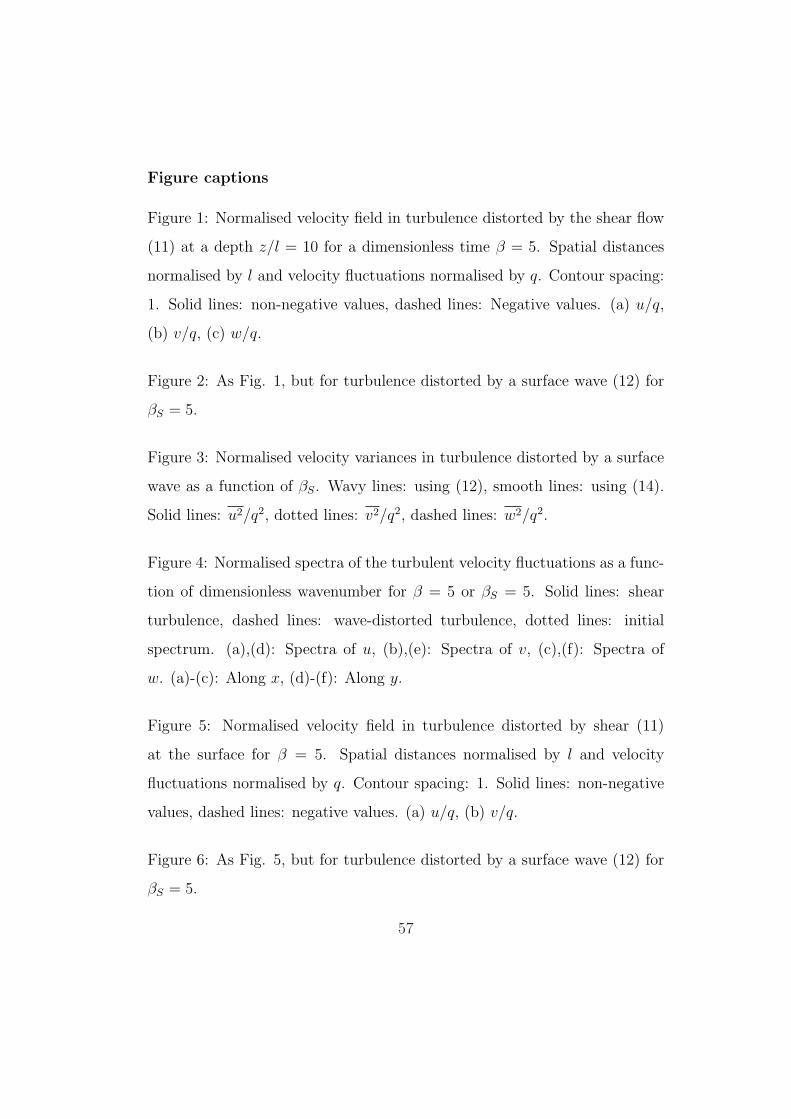
Figure captions

Figure 1: Normalised velocity field in turbulence distorted by the shear flow

(11) at a depth z/l = 10 for a dimensionless time β = 5. Spatial distances

normalised by l and velocity fluctuations normalised by q. Contour spacing:

1. Solid lines: non-negative values, dashed lines: Negative values. (a) u/q,

(b) v/q, (c) w/q.

Figure 2: As Fig. 1, but for turbulence distorted by a surface wave (12) for

βS = 5.

Figure 3: Normalised velocity variances in turbulence distorted by a surface

wave as a function of βS. Wavy lines: using (12), smooth lines: using (14).

Solid lines: u2/q2, dotted lines: v2/q2, dashed lines: w2/q2.

Figure 4: Normalised spectra of the turbulent velocity fluctuations as a func-

tion of dimensionless wavenumber for β = 5 or βS = 5. Solid lines: shear

turbulence, dashed lines: wave-distorted turbulence, dotted lines: initial

spectrum. (a),(d): Spectra of u, (b),(e): Spectra of v, (c),(f): Spectra of

w. (a)-(c): Along x, (d)-(f): Along y.

Figure 5: Normalised velocity field in turbulence distorted by shear (11)

at the surface for β = 5. Spatial distances normalised by l and velocity

fluctuations normalised by q. Contour spacing: 1. Solid lines: non-negative

values, dashed lines: negative values. (a) u/q, (b) v/q.

Figure 6: As Fig. 5, but for turbulence distorted by a surface wave (12) for

βS = 5.

57

Figure 7: Tracer particles released at the surface and transported by the

turbulence over an eddy turn-over time, qt/l = 1. Distances normalised by

l. (a) Initial positions, (b) Shear turbulence at β = 5, (c) Wave-distorted

turbulence at βS = 5.

Figure 8: Schematic diagram showing what processes lead to the alignment of

surface tracers in wave-distorted turbulence and in shear turbulence. Arrows:

direction of motion, circles: tracer particles.

Figure 9: (a) Profile of the shear rate in experiment S/∞ (squares) and

experiment E/0.3 of MSM97 (circles), for a logarithmic profile with u∗ =

6.1 × 10−3ms−1 (dotted line) and for a logarithmic profile with u∗ = 0.61 ×10−3ms−1 (solid line), and of the strain rate associated with the Stokes drift

of the wave (dashed line). (b) Profile of R−1 in experiment E/0.3 of MSM97

(circles) and from (17) for u∗s = 0.61 × 10−3ms−1 (solid line) and u∗s =

6.1× 10−3ms−1 (dotted line).

Figure 10: Profiles of the normalised integral length scale and eddy turn-over

time derived from the data of MSM97. (a) Integral length scale. Dotted line:

LES data, dashed line: linear fit between z/h = 0.1 and z/h = 0.8, solid line:

z/l = 1. (b) Eddy turn-over time. Dotted line: LES data, solid line: linear

fit between z/h = 0.1 and z/h = 0.8.

Figure 11: Dimensionless time βS used in the RDT and KST models as a

function of depth from (27) using the data from experiment E0.3 of MSM97

(solid line) and using the surface eddy turn-over time everywhere (dotted

line).

58

Figure 12: Profiles of the normalised turbulent velocity variances. Symbols:

data from MSM97, lines: RDT of turbulence distorted by a surface wave.

Solid lines and circles: u2/(2/3K), dotted lines and squares: v2/(2/3K),

dashed lines and diamonds: w2/(2/3K). (a) Depth-dependent eddy turn-

over time, (b) Constant eddy turn-over time, (c) Only with blocking effect

(note that the solid and dotted lines are superimposed).

Figure 13: Velocity fluctuations in turbulence distorted by a surface wave

at z/l = 0.40 from KST for the conditions of experiment E/0.3 of MSM97.

Dark shading: positive values, light shading: negative values. Contour spac-

ings are equivalent to those used in MSM97: u − (±0.41,±1.03,±1.55),

v − (±0.62,±1.55,±2.59), w − (±0.52,±1.03,±1.55) (see text for details).

(a) u/q field, (b) v/q field, (c) w/q field.

59