Azimuthal structure of turbulence in high Reynolds … structure of turbulence in high Reynolds...

J. Fluid Mech. (2008), vol. 615, pp. 121–138. c© 2008 Cambridge University Press

doi:10.1017/S0022112008003492 Printed in the United Kingdom

121

Azimuthal structure of turbulence in highReynolds number pipe flow

SEAN C. C. BAILEY1, MARCUS HULTMARK1,ALEXANDER J. SMITS1 AND MICHAEL P. SCHULTZ2

1Department of Mechanical and Aerospace Engineering, Princeton University,Princeton, NJ 08544, USA

2Department of Naval Architecture and Ocean Engineering, U.S. Naval Academy,Annapolis, MD 21402, USA

(Received 26 November 2007 and in revised form 16 July 2008)

Two-point hot-wire measurements of streamwise velocity were performed in thelogarithmic and wake regions of turbulent pipe flow for Reynolds numbers, based onpipe diameter, ranging from 7.6 × 104 to 8.3 × 106 at four wall-normal positions withazimuthal probe separation. The azimuthal correlations were found to be consistentwith the presence of very large-scale coherent regions of low-wavenumber, low-momentum fluid observed in previous studies of wall-bounded flows and were foundto be independent of changing Reynolds number and surface roughness effects. At theedge of the logarithmic layer the azimuthal scale determined from the correlationswas found to be similar to that observed for channel flows but larger than thatobserved for boundary layers, inconsistent with the concept of a universal logarithmicregion. As the wall-normal position increased outside the logarithmic layer, there wasa decrease in azimuthal scale relative to that of channel flow. Using cross-spectralanalysis, high-wavenumber motion was found to grow azimuthally with wall-normaldistance at a faster rate than the low-wavenumber motions.

1. IntroductionTurbulent wall-bounded flows can be classified as being either external or internal,

depending on the boundary conditions. Some of the simplest (and most widelystudied) examples are the flat plate boundary layer, fully developed rectangularchannel flow and fully developed pipe flow. The different boundary conditions createslightly different flow behaviour in each case; in zero-pressure-gradient boundarylayers momentum is lost to wall shear, and the flow continuously develops streamwise,whereas (after sufficient development length) the streamwise pressure gradients in pipeand channel flows balance the wall shear, and the flow is fully developed. Differingboundary conditions also lead to differences in the structure of turbulence in theouter layer of the wall flow, the most prominent being the intermittency resultingfrom entrainment of irrotational free stream fluid into the boundary layer.

Recent flow visualizations, numerical studies and particle image velocimetry (PIV)investigations have expanded our knowledge of coherent structures in wall flows anddemonstrated the existence of asymmetric and symmetric hairpin vortical structures(see for example Head & Bandyopadhyay 1981; Robinson 1991; Meinhart & Adrian1995). These structures are believed to grow through merging with other hairpinstructures of similar scale (Tomkins & Adrian 2003) with the oldest and largeststructures extending as far as the wall layer height δ.

122 S. C. C. Bailey, M. Hultmark, A. J. Smits and M. P. Schultz

Single hairpin structures have also been observed to spawn trailing hairpinstructures, which tend to travel at the same convective velocity (Zhou et al. 1999).Termed ‘vortex packets’, these groups of hairpin structures have a streamwise scaleof approximately 2–3δ and have been associated with the bulges of turbulent fluid atthe edge of the wall layer, also described as ‘large-scale motions or LSMs’, by Kim &Adrian (1999), Guala, Hommema & Adrian (2006) and Balakumar & Adrian (2007).The streamwise alignment of the hairpin structures within the packets induces long,narrow regions of low streamwise momentum (Adrian, Meinhart & Tomkins 2000;Ganapathisubramani, Longmire & Marusic 2003; Tomkins & Adrian 2003; Hutchins,Hambleton & Marusic 2005).

Very large-scale regions of low streamwise momentum more than 20δ long havealso been observed in the logarithmic and wake regions of wall flows, althoughspanwise/azimuthal meandering of these regions makes it difficult to determinetheir typical streamwise extent (Hutchins, Ganapathisubramani & Marusic 2004;Hutchins & Marusic 2007a; Monty et al. 2007). Referred to as ‘superstructures’(Hutchins & Marusic 2007a) or ‘very large-scale motions (VLSMs)’ (Kim & Adrian1999; Tomkins & Adrian 2005; Guala et al. 2006; Balakumar & Adrian 2007) thesestructures are much longer than the sub-layer streaks and scale on outer variables.They are believed to be associated with the long streamwise modes observed in DNSdata at large spanwise wavenumbers (Hoyas & Jimenez 2006). Although it has beenproposed that these VLSMs are caused by pseudo-streamwise alignment of hairpinpackets (Kim & Adrian 1999), it has also been suggested they could be formed bylinear or nonlinear instabilities (e.g. Del Alamo & Jimenez 2006).

Spectral analysis of the VLSMs indicates that they have a non-negligiblecontribution to the turbulent kinetic energy and Reynolds stress production (Gualaet al. 2006; Balakumar & Adrian 2007) which separate them from the inactive motionsproposed by Townsend (1976). Careful analysis of DNS data has also revealed thefootprint of the outer-scaled VLSM within the inner-scaled inner layer (Hoyas &Jimenez 2006; Hutchins & Marusic 2007a ,b).

Most of the previous work investigating the spanwise scales of LSMs and VLSMshas concentrated on smooth-walled boundary layer and channel flows. However, theparticular boundary conditions experienced in pipe flow may be expected to changethe nature of the azimuthal scales of these motions. For example in channels andboundary layers the spanwise scale determined from the spanwise correlation (whichcontains contributions from both LSMs and VLSMs) increases monotonically withwall-normal position up to the maximum of δ or half the channel height, whereasgeometrical considerations in pipe flow imply that spanwise scales cannot increase inthe same way.

To investigate the azimuthal structure within pipe flow, Monty et al. (2007) used arake of hot-wire probes and found that at the outer edge of the logarithmic region theazimuthal scale was nearly identical to that determined from similar measurementsin channel flow. The measurements were confined to a single wall-normal position inthe pipe, and hence the change in azimuthal scales with wall-normal distance couldnot be investigated.

Therefore, the objective of the current study is to investigate the wall-normaldependence of the azimuthal scale of the large-scale and very large-scale structureswithin the logarithmic and wake regions of pipe flow for a large range of Reynoldsnumber based on pipe diameter D from ReD = 7.6 × 104 to ReD = 8.3 × 106, whereReD = D〈U〉/ν; 〈U〉 is the area-averaged velocity, and ν is the kinematic viscosity.As well as providing the opportunity to investigate the ReD dependence over a much

Azimuthal scale of turbulence in pipe flow 123

Pumpingsection

Heatexchanger

Return leg

Flow-conditioningsection

Test legPrimary testsection

Diffuser section

To motor

34 m

1.5 mTest pipe

flow

flow

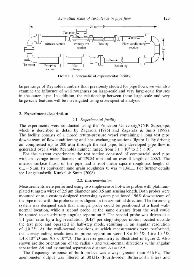
Figure 1. Schematic of experimental facility.

larger range of Reynolds numbers than previously studied for pipe flows, we will alsoexamine the influence of wall roughness on large-scale and very large-scale featuresin the outer layer. In addition, the relationship between these large-scale and verylarge-scale features will be investigated using cross-spectral analysis.

2. Experiment description2.1. Experimental facility

The experiments were conducted using the Princeton University/ONR Superpipe,which is described in detail by Zagarola (1996) and Zagarola & Smits (1998).The facility consists of a closed return-pressure vessel containing a long test pipedownstream of flow-conditioning and heat-exchanging sections (figure 1). By drivingair compressed up to 200 atm through the test pipe, fully developed pipe flow isgenerated over a wide Reynolds number range, from 3.1 × 104 to 3.5 × 107.

For the current experiments the test section consisted of commercial steel pipewith an average inner diameter of 129.84 mm and an overall length of 200D. Theinterior surface finish of the pipe had a root mean square roughness height ofkrms = 5 μm. Its equivalent sand grain roughness ks was � 1.6krms. For further detailssee Langelandsvik, Kunkel & Smits (2008).

2.2. Instrumentation

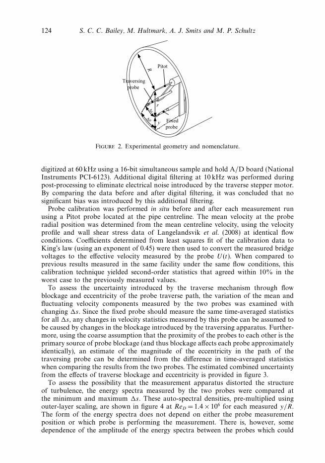
Measurements were performed using two single-sensor hot-wire probes with platinum-plated tungsten wires of 2.5 μm diameter and 0.5 mm sensing length. Both probes weremounted onto a custom-designed traversing system positioned 196D downstream ofthe pipe inlet, with the probe sensors aligned in the azimuthal direction. The traversingsystem was designed such that a single probe could be positioned at a fixed wall-normal location, while a second probe at the same distance from the wall couldbe rotated to an arbitrary angular separation θ . The second probe was driven at a1:1 gear ratio by a high-resolution (0.45◦ per step) stepper motor, located outsidethe test pipe and operated in half-step mode, resulting in an angular resolutionof ±0.23◦. At the wall-normal positions at which measurements were performed,the corresponding resolutions in probe separation were 1.8 × 10−3D, 1.6 × 10−3D,1.4 × 10−3D and 9.8 × 10−4D. The traverse geometry is illustrated in figure 2. Alsoshown are the orientations of the radial r and wall-normal directions y, the angularseparation �θ and azimuthal separation distance �s = r�θ .

The frequency response of both probes was always greater than 65 kHz. Theanemometer output was filtered at 30 kHz (fourth-order Butterworth filter) and


R

r

y Fixedprobe

Traversingprobe

Pitot

ΔsΔθ

Figure 2. Experimental geometry and nomenclature.

digitized at 60 kHz using a 16-bit simultaneous sample and hold A/D board (NationalInstruments PCI-6123). Additional digital filtering at 10 kHz was performed duringpost-processing to eliminate electrical noise introduced by the traverse stepper motor.By comparing the data before and after digital filtering, it was concluded that nosignificant bias was introduced by this additional filtering.

Probe calibration was performed in situ before and after each measurement runusing a Pitot probe located at the pipe centreline. The mean velocity at the proberadial position was determined from the mean centreline velocity, using the velocityprofile and wall shear stress data of Langelandsvik et al. (2008) at identical flowconditions. Coefficients determined from least squares fit of the calibration data toKing’s law (using an exponent of 0.45) were then used to convert the measured bridgevoltages to the effective velocity measured by the probe U (t). When compared toprevious results measured in the same facility under the same flow conditions, thiscalibration technique yielded second-order statistics that agreed within 10% in theworst case to the previously measured values.

To assess the uncertainty introduced by the traverse mechanism through flowblockage and eccentricity of the probe traverse path, the variation of the mean andfluctuating velocity components measured by the two probes was examined withchanging �s. Since the fixed probe should measure the same time-averaged statisticsfor all �s, any changes in velocity statistics measured by this probe can be assumed tobe caused by changes in the blockage introduced by the traversing apparatus. Further-more, using the coarse assumption that the proximity of the probes to each other is theprimary source of probe blockage (and thus blockage affects each probe approximatelyidentically), an estimate of the magnitude of the eccentricity in the path of thetraversing probe can be determined from the difference in time-averaged statisticswhen comparing the results from the two probes. The estimated combined uncertaintyfrom the effects of traverse blockage and eccentricity is provided in figure 3.

To assess the possibility that the measurement apparatus distorted the structureof turbulence, the energy spectra measured by the two probes were compared atthe minimum and maximum �s. These auto-spectral densities, pre-multiplied usingouter-layer scaling, are shown in figure 4 at ReD =1.4 × 106 for each measured y/R.The form of the energy spectra does not depend on either the probe measurementposition or which probe is performing the measurement. There is, however, somedependence of the amplitude of the energy spectra between the probes which could


Δs/R

Unc

erta

inty

(%

)

0 0.5 1.0 1.5 2.0Δs/R

0 0.5 1.0 1.5 2.0

1

2

3

4

5(a) (b)

Figure 3. Estimated uncertainty in (a) mean velocity and (b) standard deviation of velocitybecause of combined effects of eccentricity and probe blockage at �, y/R = 0.1; �, y/R = 0.2;�, y/R = 0.3; �, y/R = 0.5.

kRΦ

/u2 τ

0

0.5

1.0(a) (b)

kRΦ

/u2 τ

0

0.5

1.0(c) (d)

kR

10–1 100 101 102 103

kR

10–1 100 101 102 103

Figure 4. Pre-multiplied auto-spectral density kRΦ measured at ReD = 1.4 × 106 at minimumprobe separation (�) and maximum probe separation (�) by fixed (hollow symbols) andtraversing (filled symbols) probe at (a) y/R = 0.1, (b) y/R =0.2, (c) y/R = 0.3 and (d) y/R = 0.5.

be attributed to the effects of traverse blockage and eccentricity. Since the azimuthaland wall-normal scales of the structures of interest in this study are on the orderof 0.5R, these small distortions in the flow field should not affect our conclusionsregarding the behaviour of these structures.

2.3. Measurement conditions

Measurements were performed at ReD = 7.6 × 104 to 8.3 × 106, encompassingthe hydraulically smooth, transitionally rough and fully rough flow regimes.


ReD Reτ 〈U〉 (m s−1) δν (μm) k+s λ Flow type

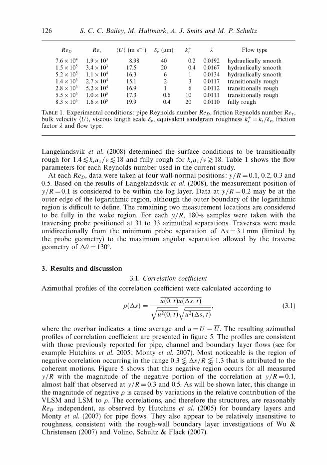
7.6 × 104 1.9 × 103 8.98 40 0.2 0.0192 hydraulically smooth1.5 × 105 3.4 × 103 17.5 20 0.4 0.0167 hydraulically smooth5.2 × 105 1.1 × 104 16.3 6 1 0.0134 hydraulically smooth1.4 × 106 2.7 × 104 15.1 2 3 0.0117 transitionally rough2.8 × 106 5.2 × 104 16.9 1 6 0.0112 transitionally rough5.5 × 106 1.0 × 105 17.3 0.6 10 0.0111 transitionally rough8.3 × 106 1.6 × 105 19.9 0.4 20 0.0110 fully rough

Table 1. Experimental conditions: pipe Reynolds number ReD , friction Reynolds number Reτ ,bulk velocity 〈U〉, viscous length scale δν , equivalent sandgrain roughness k+

s = ks/δν , frictionfactor λ and flow type.

Langelandsvik et al. (2008) determined the surface conditions to be transitionallyrough for 1.4 � ksuτ /ν � 18 and fully rough for ksuτ /ν � 18. Table 1 shows the flowparameters for each Reynolds number used in the current study.

At each ReD , data were taken at four wall-normal positions: y/R = 0.1, 0.2, 0.3 and0.5. Based on the results of Langelandsvik et al. (2008), the measurement position ofy/R =0.1 is considered to be within the log layer. Data at y/R = 0.2 may be at theouter edge of the logarithmic region, although the outer boundary of the logarithmicregion is difficult to define. The remaining two measurement locations are consideredto be fully in the wake region. For each y/R, 180-s samples were taken with thetraversing probe positioned at 31 to 33 azimuthal separations. Traverses were madeunidirectionally from the minimum probe separation of �s = 3.1mm (limited bythe probe geometry) to the maximum angular separation allowed by the traversegeometry of �θ = 130◦.

3. Results and discussion3.1. Correlation coefficient

Azimuthal profiles of the correlation coefficient were calculated according to

ρ(�s) =u(0, t)u(�s, t)√

u2(0, t)

√u2(�s, t)

, (3.1)

where the overbar indicates a time average and u = U − U . The resulting azimuthalprofiles of correlation coefficient are presented in figure 5. The profiles are consistentwith those previously reported for pipe, channel and boundary layer flows (see forexample Hutchins et al. 2005; Monty et al. 2007). Most noticeable is the region ofnegative correlation occurring in the range 0.3 � �s/R � 1.3 that is attributed to thecoherent motions. Figure 5 shows that this negative region occurs for all measuredy/R with the magnitude of the negative portion of the correlation at y/R = 0.1,almost half that observed at y/R = 0.3 and 0.5. As will be shown later, this change inthe magnitude of negative ρ is caused by variations in the relative contribution of theVLSM and LSM to ρ. The correlations, and therefore the structures, are reasonablyReD independent, as observed by Hutchins et al. (2005) for boundary layers andMonty et al. (2007) for pipe flows. They also appear to be relatively insensitive toroughness, consistent with the rough-wall boundary layer investigations of Wu &Christensen (2007) and Volino, Schultz & Flack (2007).


(b)(a)

ρ

0

0.5

1.0

0

0.5

1.0(c) (d)

Δs/R Δs/R

ρ

0 0.5 1.0 1.5 2.0 0 0.5 1.0 1.5 2.0

Figure 5. Correlation coefficient measured at (a) y/R =0.1, (b) y/R =0.2, (c) y/R =0.3 and(d) y/R =0.5; �, ReD = 7.6 × 104; �, 1.5 × 105; �, 5.2 × 105; �, 1.4 × 106; �, 2.8 × 106; �,5.5 × 106; �, 8.3 × 106.

To visualize the variation of ρ(�s) with wall-normal position and to illustrate howthe azimuthal scales relate to the pipe geometry, isocontours of ρ(�s) are shown infigure 6. This figure further illustrates the similarity of the azimuthal correlations overa ReD range spanning two orders of magnitude and surface roughness conditionsvarying from hydraulically smooth to fully rough.

Ganapathisubramani et al. (2003) introduced a spanwise width scale lz, definedas the range of spanwise displacement where ρ(�s) > 0.05, to help summarize suchcorrelations as those shown in figure 5. The spanwise width scale determined fromfigure 5 is compared to previous measurements for boundary layer, channel and pipeflows in figure 7(a) (adapted from figure 6a in Monty et al. (2007) with additionaldata), where δ represents the height of boundary layer, half-height of the channel orpipe radius respectively.

Although there is considerable scatter, particularly at y/R = 0.2, the spanwise widthscales of the pipe and channel flows were found to be similar within the logarithmiclayer, but both were twice that observed in the boundary layers. Note that, sincethe motions scale on outer variables, they therefore depend on the type of flow(boundary layer, channel or pipe). Also, the azimuthal scales contributing to lz withinthe log layer are influenced by these outer-scale motions, resulting in a measurablecontribution to the Reynolds stresses (Guala et al. 2006; Balakumar & Adrian 2007),so the differences observed in the scaling of lz within the logarithmic layer areinconsistent with the notion that the turbulence structure within the logarithmic layerat high Reynolds numbers is universal.

For y/R > 0.2, the azimuthal width in pipe flows decreases relative to the widthobserved in channel flows. This reflects the increased spatial constraints imposed in


–0.20 –0.10 0 0.10 0.20 0.30 0.40 0.50 0.60 0.70 0.80 0.90 1.00

ReD = 7.6 × 104 ReD = 1.5 × 105 ReD = 5.2 × 105

ReD = 1.4 × 106 ReD = 2.8 × 106

ReD = 8.3 × 106

ReD = 5.5 × 106

Figure 6. Isocontours of ρ(�s) for each ReD investigated. The azimuthal range of the datais expanded by utilizing the even-functioned nature of 2-point correlations.

y/δ

l z/δ

0 0.2 0.4 0.6 0.8 1.0 1.2

0.5

1.0

(a)

y/R

l z/(

2πr)

0.2 0.4 0.60

0.1

0.2

0.3(b)

Figure 7. Dependence of the spanwise width scale lz when (a) scaled by δ and (b) scaledby 2πr . Here δ represents the height of boundary layer, half-height of the channel or pipe

radius. Channel: �, Monty et al. (2007). Channel DNS: �, data of Del Alamo et al. (2004).Boundary layer: �, Tomkins & Adrian (2003); �, Krogstad & Antonia (1994); �, Hutchinset al. (2005); �, Hutchins & Marusic (2007a); ×, Volino et al. (2007). Rough-wall boundarylayer: �, Volino et al. (2007). Pipe: �, Monty et al. (2007). Present results: �, ReD =7.6 × 104;�, 1.5 × 105; �, 5.2 × 105; , 1.4 × 106; , 2.8 × 106; �, 5.5 × 106; , 8.3 × 106.


pipe flow as y approaches R. The strong influence of geometry on the azimuthalscales is further illustrated in figure 7(b), which shows that when scaled by the localpipe circumference, lz grows approximately linearly with y/R.

3.2. Cross-spectra

Two-point correlations, such as those shown in figure 5, contain contributions frommotions over a wide range of scales which, through the averaging process, can obscurethe azimuthal scale of LSMs and VLSMs. Hence, to investigate the dependence ofthe two-point correlations on streamwise wavenumber k, the one-sided cross-spectraldensity G, was calculated from

G(�s, k) = F ∗(0, k)F (�s, k), (3.2)

where F indicates the Fourier transform of the velocity signal, and ∗ indicates acomplex conjugate. Bendat & Piersol (2000) show that

ρ(�s) =

∫ ∞

0

Re[G(�s, k)] dk, (3.3)

where Re indicates the real component. Thus, the quantity

Ψ (�s, k) = Re[G(�s, k)]

√u2(0, t)

√u2(�s, t) (3.4)

can be defined such that Ψ (0, k) = Φ(k), the auto-spectral density measured by thefixed probe. Thus, Ψ (�s, k) can be thought of as the wavenumber distribution of thecorrelation coefficient at azimuthal separation �s.

Isocontours of pre-multiplied cross-spectral density using outer layer scaling kRΨ ,are shown in figure 8 at ReD =1.4 × 106 for each measured y/R. The correspondingpre-multiplied auto-spectra measured by the fixed probe are also shown. Only resultsat ReD =1.4 × 106 are shown in figure 8, since similar results were observed at allReynolds numbers.

The pre-multiplied auto-spectra in the current results are consistent with thosepreviously reported by Kim & Adrian (1999). The most notable feature is the presenceof two distinct peaks at kR ≈ 0.3 − 0.8 and kR ≈ 2 − 5, which have been attributedby Kim & Adrian (1999) to the distribution of VLSMs and LSMs respectively. Forconvenience, the terms VLSM and LSM will also be retained here to describe themotions at the corresponding spectral peak which will be considered to indicate themost common wavenumber of the motion. Although both peaks decrease in energywith increasing y/R, the energy contained in the VLSM peak decreases at a fasterrate. Thus, within the logarithmic layer the VLSM peak is more prominent than theLSM peak, and within the outer layer the reverse is true.

The isocontours shown in figure 8 reveal a large region of negative Ψ within arange of �s corresponding to the probe separation at which the negative values areobserved in the cross-correlation results (figure 5). The azimuthal separations at whichthis negatively correlated region occurs decrease with increasing wavenumber.

At the measurement location closest to the wall, y/R =0.1, the spanwise scale ofthe negatively correlated region shows no clear delineation between the VLSMs andLSMs, but there is a noticeable inflection point in the positively correlated valuesat approximately the same wavenumber as the inflection point in the correspondingauto-spectrum. The widest structures at this wall-normal position occur at streamwisewavenumbers associated with the VLSM peak. At this wavenumber, the negativeΨ values are centred at �s/R ≈ 0.5, which coincides with the azimuthal locationof minimum ρ(�s) observed in figure 5 and by Monty et al. (2007). Thus, thepresent results clearly connect the streamwise VLSMs described by power-spectrum


Δs/R

0

0.2

0.4

0.6

0.8

1.0

1.2(a)

kRΦ

/u2 τ

10–1 100 101 102 1030

0.5

1.0

0.5

1.0

(b)

10–1 100 101 102 1030

0

0.5

1.0

Δs/R

0

0.2

0.4

0.6

0.8

1.0

1.2(c)

kR

kRΦ

/u2 τ

10–1 100 101 102 1030

0.5

1.00

0.2

0.4

0.6

0.8

1.2

1.0

(d)

kR

10–1 100 101 102 1030

0.5

1.0

Figure 8. Contours of pre-multiplied cross-spectral density kRΨ/u2τ at ReD = 1.4 × 106 for

wall-normal locations (a) y/R = 0.1, (b) y/R = 0.2, (c) y/R = 0.3 and (d) y/R = 0.5. The contourlevels are separated by 0.025; negative contours are shown as broken contour lines, and contourlevels at zero are not shown for clarity. The corresponding pre-multiplied auto-spectral densitykRΦ is shown below each contour plot. Wavenumbers of very large-scale and large-scale peaksindicated by dashed lines.


analysis (Kim & Adrian 1999; Guala et al. 2006; Balakumar & Adrian 2007) to theazimuthal/spanwise scale of ‘superstructures’ found using correlations and conditionalaveraging (see for example Hutchins & Marusic 2007a ,b; Monty et al. 2007).

As wall distance increases, the energy contained within the VLSMs decreasesrelative to that contained within the LSMs. Correspondingly, the negatively correlatedregion at the LSM wavenumbers grows azimuthally and becomes distinct from thatof the VLSM wavenumbers, resulting in the appearance of two separate regionsof values negatively correlated by y/R = 0.5. Simultaneously, as y/R increases, theazimuthal scale at LSM wavenumbers approximately triples relative to the scale atLSM wavenumbers at y/R =0.1, reflecting azimuthal growth of the LSM. For thesame y/R range, the distribution of negative Ψ at VLSM wavenumbers appears tobe independent of wall-normal distance.

An attempt to separate the contribution of the VLSM and LSM to ρ was made byspectral filtration of the cross-correlation, using

ρvl(�s) =

∫ kcut

0

Re[G(�s, k)] dk, (3.5)

where ρvl contains the contributions to ρ primarily from the VLSM, and

ρl(�s) =

∫ ∞

kcut

Re[G(�s, k)] dk, (3.6)

contains the contributions primarily from the LSM. The values of kcut depend onwall-normal position and were selected using the location of the inflection in thecorresponding auto-spectrum (as evident in figure 8). Here kcut is considered to bea wavenumber below which the VLSM have the greatest energy contribution andabove which the LSM have the greatest contribution. The selected values for kcutR

were 1.5, 1.2, 0.8 and 0.6 for y/R = 0.1, 0.2, 0.3 and 0.5 respectively.The resulting azimuthal distributions of ρvl and ρl for all measured wavenumbers

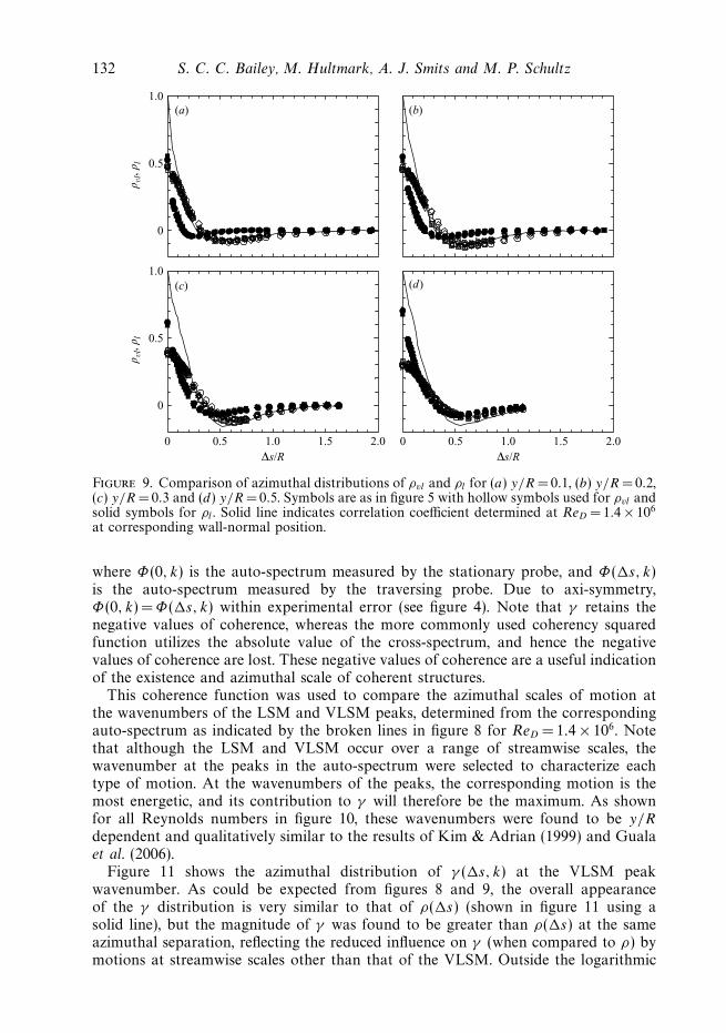
are compared to the azimuthal distribution of ρ in figure 9. In general, the magnitudeof ρvl is larger than that of ρl except at small very small �s, where there isan increased contribution to ρ from small-scale motions. Figure 9 clearly showsdifferences in the azimuthal and wall-normal dependence of the VLSM and LSM.Figure 9 also highlights the observation that any width scale determined from thecross-correlation is not a good indicator of the width of either VLSM or LSM becausethe contribution of each type of motion to ρ varies with wall-normal position. Aty/R = 0.1, where the VLSM has more energy than the LSM, the VLSM providesthe greatest contribution to the cross-correlation, whereas at y/R =0.5, the energycontained in the LSM relative to that contained in the VLSM increases to the pointat which its corresponding contribution to ρ is approximately equal to that of theVLSM. Note that the increase in azimuthal width of the LSM, combined with theincreased energy contained within them, causes the increase in the magnitude of thenegative ρ values with the y/R observed in figure 5.

3.3. Coherence function

To further investigate and quantify the differences in behaviour of the azimuthal scaleof the VLSMs and LSMs, a coherence function γ (�s, k) is introduced as

γ (�s, k) =Ψ (�s, k)

Φ1/2(0, k)Φ1/2(�s, k), (3.7)


ρvl

, ρl

0

0.5

1.0(a) (b)

ρvl

, ρl

0

0.5

1.0(c) (d)

Δs/R0 0.5 1.0 1.5 2.0

Δs/R0 0.5 1.0 1.5 2.0

Figure 9. Comparison of azimuthal distributions of ρvl and ρl for (a) y/R = 0.1, (b) y/R = 0.2,(c) y/R = 0.3 and (d) y/R = 0.5. Symbols are as in figure 5 with hollow symbols used for ρvl andsolid symbols for ρl . Solid line indicates correlation coefficient determined at ReD = 1.4 × 106

at corresponding wall-normal position.

where Φ(0, k) is the auto-spectrum measured by the stationary probe, and Φ(�s, k)is the auto-spectrum measured by the traversing probe. Due to axi-symmetry,Φ(0, k) = Φ(�s, k) within experimental error (see figure 4). Note that γ retains thenegative values of coherence, whereas the more commonly used coherency squaredfunction utilizes the absolute value of the cross-spectrum, and hence the negativevalues of coherence are lost. These negative values of coherence are a useful indicationof the existence and azimuthal scale of coherent structures.

This coherence function was used to compare the azimuthal scales of motion atthe wavenumbers of the LSM and VLSM peaks, determined from the correspondingauto-spectrum as indicated by the broken lines in figure 8 for ReD = 1.4 × 106. Notethat although the LSM and VLSM occur over a range of streamwise scales, thewavenumber at the peaks in the auto-spectrum were selected to characterize eachtype of motion. At the wavenumbers of the peaks, the corresponding motion is themost energetic, and its contribution to γ will therefore be the maximum. As shownfor all Reynolds numbers in figure 10, these wavenumbers were found to be y/R

dependent and qualitatively similar to the results of Kim & Adrian (1999) and Gualaet al. (2006).

Figure 11 shows the azimuthal distribution of γ (�s, k) at the VLSM peakwavenumber. As could be expected from figures 8 and 9, the overall appearanceof the γ distribution is very similar to that of ρ(�s) (shown in figure 11 using asolid line), but the magnitude of γ was found to be greater than ρ(�s) at the sameazimuthal separation, reflecting the reduced influence on γ (when compared to ρ) bymotions at streamwise scales other than that of the VLSM. Outside the logarithmic


y/R

kR

0 0.2 0.4 0.6

1

2

3

4

5

Figure 10. Wavenumbers of very large-scale peaks (hollow symbols) and large-scale peaks(solid symbols) determined from auto-spectra. Symbols are as in figure 5.

γ

0

0.5

1.0(a) (b)

γ

0

0.5

1.0(c) (d)

Δs/R

0 0.5 1.0 1.5 2.0

Δs/R

0 0.5 1.0 1.5 2.0

Figure 11. Azimuthal distribution of coherence function γ at VLSM wavenumbers measuredat (a) y/R = 0.1, (b) y/R = 0.2, (c) y/R = 0.3 and (d) y/R = 0.5. Symbols are as in figure 5.Solid lines indicate azimuthal distribution of ρ at ReD = 1.4 × 106 for the corresponding y/Rposition.

layer (y/R > 0.1), there is very little change in the γ distributions with wall-normaldistance, indicating little change in the azimuthal scale of the VLSM.

Figure 12 shows the azimuthal distribution of γ (�s, k) at the LSM peak in theauto-spectrum. Note that at y/R = 0.1, the LSM peak was not clearly defined formost of the Reynolds numbers (as evident in figure 8a for ReD = 1.4 × 106). Sincethe wavenumber of the LSM peak was found to show little ReD dependence, aty/R = 0.1 the azimuthal distribution of γ for all ReD values was determined at theLSM wavenumber found for ReD = 7.6 × 104, which had a clearly defined peak. Theoverall appearance of the azimuthal distribution of γ at the LSM peak wavenumber


γ

0

0.5

1.0

γ

0

0.5

1.0

(a) (b)

(c) (d)

Δs/R0 0.5 1.0 1.5 2.0

Δs/R0 0.5 1.0 1.5 2.0

Figure 12. Azimuthal distribution of coherence function γ at LSM wavenumbers measuredat (a) y/R = 0.1, (b) y/R = 0.2, (c) y/R = 0.3 and (d) y/R = 0.5. Symbols are as in figure 5.Solid lines indicate azimuthal distribution of ρ at ReD = 1.4 × 106 for the corresponding y/Rposition.

y/R

l vl/R

, ll/R

0 0.2 0.4 0.6y/R

0 0.2 0.4 0.6

0.2

0.4

0.6

0.8(a)

1.0

1.5

2.0

(b)

l vl/l

l

Figure 13. (a) Spanwise width scales lvl and ll as functions of y/R; hollow symbols lvl; solidsymbols ll . (b) Ratio of lvl to ll . Symbols are as in figure 5.

in figure 12 is similar to that observed at the VLSM peak wavenumber shown infigure 11, although the magnitude of γ is reduced for the LSM. As also shown infigure 9 and unlike the previously noted behaviour of the VLSM, there is a strongy/R dependence evident for the LSM.

The y/R dependence of the azimuthal scale of the VLSM and LSM structurescan be quantified and compared through definition of the spanwise width scales lvl

and ll which, following the definition of lz, are defined as the azimuthal separationover which γ > 0.05 at the VLSM and LSM peak wavenumber respectively. Seefigures 13(a) and 13(b). The azimuthal scale of the VLSM was found to be largerthan the LSM at all y/R, but the ratio of their sizes decreases with wall distance: aty/R =0.1, lvl/ ll ≈ 2, and at y/R = 0.5 the ratio decreases to about 1.2 (figure 13b).


This decrease in relative size is clearly due to the faster growth rate of the LSM withy/R (figure 13a). As the wall distance increases, however, the rate of growth of theLSM decreases, and lvl/ ll appears to asymptote towards unity.

Previous researchers (see Zhou et al. 1999 for example) have observed that hairpinvortices can group into packets of streamwise aligned hairpins which travel at acommon convection velocity. Within the logarithmic layer these hairpin packets cancontain a wide range of scales, with only the oldest and largest of these structurespersisting into the wake region, where they appear as turbulent bulges in the outerlayer.

It has also been proposed that when these packets of hairpin vortices becomestreamwise aligned, they result in the very long, low-momentum regions of thesuperstructures/VLSMs (Kim & Adrian 1999; Adrian et al. 2000; Guala et al. 2006).If this were the case, it may be expected that the azimuthal scales of the LSMs andVLSMs would be similar at all wall-normal positions. The current results, however,show that the VLSMs are almost twice as wide as the LSMs at y/R = 0.1 and are still25% larger at y/R = 0.5. This disparity of the spanwise scales is inconsistent with thestreamwise alignment of several hairpin packets being the source of the VLSM, unlessonly the largest hairpin packets in the wake region (y/R > 0.5) align to produce theVLSM. In pipe flows, it would seem that the largest hairpin packets have a higherprobability of alignment than the smaller packets because of increased azimuthalconfinement at large y/R. The counter-rotating legs of these largest hairpin packetswould then induce the VLSM at smaller y/R wall heights. This ‘top-down’ behaviouris supported by the outer scaling of the correlations and the relative insensitivity ofthe azimuthal correlations to the roughness conditions within the pipe. Hutchins &Marusic (2007b) have shown that the VLSM motions can be detected even within thebuffer region. This influence of the outer-scaled VLSM near the wall could contributeto the poor scaling of the ReD dependent near wall peak of u2/u2

τ when scaled oninner variables (see Morrison et al. 2004 for example).

Such a top-down imposition of the VLSM could also explain the difference inazimuthal or spanwise scales within the logarithmic layer observed between theinternal channel/pipe flows and the external boundary layer flows. As observed byMonty et al. (2007), for internal flows hairpin structures have been found to regularlyproject further into the outer layer than the boundary layers (Ganapathisubramaniet al. 2003), which could result in azimuthally larger hairpin packets within the outerlayer. This result would, in turn, create larger VLSMs. If alignment of these large-scale, outer-layer structures are the source of the VLSM, then the resulting VLSMimposed within the logarithmic layer can then be expected to be of wider scale forpipe/channel flows relative to the spanwise scale of the VLSM within the boundarylayer.

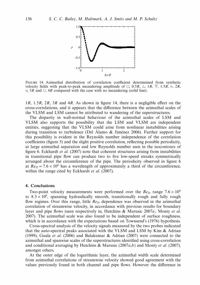
Azimuthal meandering of the VLSM as observed by Hutchins & Marusic (2007a)and Monty et al. (2007) must also be considered when interpreting the results. Givensufficient magnitude, such meandering could cause the VLSM to appear wider in thecross-spectral analysis. This artificial increase in the azimuthal scales would have agreater effect on the VLSM relative to the LSM due to their longer streamwise lengthscale and hence would cause the VLSM to appear wider in time-averaged statistics.To investigate the potential influence of meander on the statistics, the syntheticeddy analysis of Hutchins & Marusic (2007a) was repeated using 200 ensembles of50 structures having azimuthal width of 0.5R and normally distributed streamwiselength scale of maximum length 20R. Cross-correlations were calculated of syntheticeddy velocity fields with imposed peak to peak meandering amplitudes of 0R, 0.5R,


Δs/R

ρ

0 1 2–1.0

–0.5

0

1.0

0.5

Figure 14. Azimuthal distribution of correlation coefficient determeined from syntheticvelocity fields with peak-to-peak meandering amplitude of �, 0.5R, �, 1R, �, 1.5R, �, 2R,�, 3R and �, 4R compared with the case with no meandering (solid line).

1R, 1.5R, 2R, 3R and 4R. As shown in figure 14, there is a negligible effect on thecross-correlations, and it appears that the difference between the azimuthal scales ofthe VLSM and LSM cannot be attributed to wandering of the superstructures.

The disparity in wall-normal behaviour of the azimuthal scales of LSM andVLSM also supports the possibility that the LSM and VLSM are independententities, suggesting that the VLSM could arise from nonlinear instabilities arisingduring transition to turbulence (Del Alamo & Jimenez 2006). Further support forthis possibility is evident in the Reynolds number independence of the correlationcoefficients (figure 5) and the slight positive correlation, reflecting possible periodicity,at large azimuthal separation and low Reynolds number seen in the isocontours offigure 6. Eckhardt et al. (2007) note that coherent structures arising from instabilitiesin transitional pipe flow can produce two to five low-speed streaks symmetricallyarranged about the circumference of the pipe. The periodicity observed in figure 6at ReD = 7.6 × 104 has a wavelength of approximately a third of the circumference,within the range cited by Eckhardt et al. (2007).

4. ConclusionsTwo-point velocity measurements were performed over the ReD range 7.6 × 104

to 8.3 × 106, spanning hydraulically smooth, transitionally rough and fully roughflow regimes. Over this range, little ReD dependence was observed in the azimuthalcorrelation of streamwise velocity, in accordance with previous results for boundarylayer and pipe flows (seen respectively in, Hutchins & Marusic 2007a; Monty et al.2007). The azimuthal scale was also found to be independent of surface roughness,which is in accordance with the expectations based on Townsend’s (1976) hypothesis.

Cross-spectral analysis of the velocity signals measured by the two probes indicatedthat the auto-spectral peaks associated with the VLSM and LSM by Kim & Adrian(1999), Guala et al. (2006) and Balakumar & Adrian (2007) were connected to theazimuthal and spanwise scales of the superstructures identified using cross-correlationand conditional averaging by Hutchins & Marusic (2007a ,b) and Monty et al. (2007),amongst others.

At the outer edge of the logarithmic layer, the azimuthal width scale determinedfrom azimuthal correlations of streamwise velocity showed good agreement with thevalues previously found in both channel and pipe flows. However the difference in


the spanwise scale between the internal and external flows is inconsistent with thehypothesis that the structure of turbulence within the logarithmic region is universal.

In the wake region, the azimuthal width scale was found to be smaller than thatof channel flows because of increased geometric confinement. The azimuthal scale ofthe LSM also increased with wall-normal distance, approaching that of the VLSMwhich remained comparatively constant within the uncertainty of the measurementsas wall distance increased. This result indicates that if the VLSMs are caused by thestreamwise alignment of packets of hairpin vortices, only the largest and oldest ofthese packets align to create these motions. Disparity between the azimuthal scales ofthe LSM and VLSM could support the possibility that the VLSM arise from linearor nonlinear instabilities within the turbulent flow.

The support of two ONR (Office of Naval Research) grants (program ManagerRon Joslin) is gratefully acknowledged. Additional support for S.C.C.B was providedby the Natural Sciences and Engineering Research Council of Canada through thepostdoctoral fellowship program.

REFERENCES

Adrian, R. C., Meinhart, C. D. & Tomkins, C. D. 2000 Vortex organization in the outer region ofthe turbulent boundary layer. J. Fluid Mech. 422, 1–54.

Balakumar, B. J. & Adrian, R. J. 2007 Large- and very-large-scale motions in channel andboundary-layer flows. Phil. Trans. R. Soc. A 365, 665–681.

Bendat, J. S. & Piersol, A. G. 2000 Random Data : Analysis and Measurement Procedures . 3rd edn.Wiley Interscience.

Del Alamo, J. C. & Jimenez, J. 2006 Linear energy amplification in turbulent channels. J. FluidMech. 559, 205–213.

Del Alamo, J. C., Jimenez, J., Zandonade, P. & Moser, R. D. 2004 Scaling of the energy spectraof turbulent channels. J. Fluid Mech. 500, 135–144.

Eckhardt, B., Schneider, T. M., Hof, B. & Westerweel, J. 2007 Turbulence transition in pipeflow. Annu. Rev. Fluid Mech. 39, 447–468.

Ganapathisubramani, B., Longmire, E. K. & Marusic, I. 2003 Characteristics of vortex packetsin turbulent boundary layers. J. Fluid Mech. 478, 35–46.

Guala, M., Hommema, S. E. & Adrian, R. J. 2006 Large-scale and very-large-scale motions inturbulent pipe flow. J. Fluid Mech. 554, 521–542.

Head, M. R. & Bandyopadhyay, P. 1981 New aspects of turbulent boundary-layer structure.J. Fluid Mech. 107, 297–337.

Hoyas, S. & Jimenez, J. 2006 Scaling of the velocity fluctuations in turbulent channels up toReτ = 2003. Phys. Fluids 18(1), 011702.

Hutchins, N., Ganapathisubramani, B. & Marusic, I. 2004 Dominant spanwise fourier modesand the existence of very large scale coherence in turbulent boundary layers. In Proc. 15thAustralasian Fluid Mechanics Conference. Sydney, Australia.

Hutchins, N., Hambleton, W. T. & Marusic, I. 2005 Inclined cross-stream stereo particle imagevelocimetry measurements in turbulent boundary layers. J. Fluid Mech. 541, 21–54.

Hutchins, N. & Marusic, I. 2007a Evidence of very long meandering features in the logarithmicregion of turbulent boundary layers. J. Fluid Mech. 579, 1–28.

Hutchins, N. & Marusic, I. 2007b Large-scale influences in near-wall turbulence. Phil. Trans. R.Soc. A 365, 647–664.

Kim, K. C. & Adrian, R. J. 1999 Very large-scale motion in the outer layer. Phys. Fluids 11 (2),417–422.

Krogstad, P. A & Antonia, R. A. 1994 Structure of turbulent boundary layers on smooth andrough walls. J. Fluid Mech. 277, 1–21.

Langelandsvik, L. I., Kunkel, G. J. & Smits, A. J. 2008 Friction factor and mean velocity profilesin a commercial steel pipe. J. Fluid Mech. 595, 323–339.


Meinhart, C. D. & Adrian, R. J. 1995 On the existence of uniform momentum zones in a turbulentboundary layer. Phys. Fluids 7 (4), 694–696.

Monty, J. P., Stewart, J. A., Williams, R. C. & Chong, M. S. 2007 Large-scale features in turbulentpipe and channel flows. J. Fluid Mech. 589, 147–156.

Morrison, J. F., McKeon, B. J., Jiang, W. & Smits, A. J. 2004 Scaling of the streamwise velocitycomponent in turbulent pipe flow. J. Fluid Mech. 508, 99–131.

Robinson, S. K. 1991 Coherent motions in turbulent boundary layers. Annu. Rev. Fluid Mech. 23,601–639.

Tomkins, C. D. & Adrian, R. J. 2003 Spanwise structure and scale growth in turbulent boundarylayers. J. Fluid Mech. 490, 37–74.

Tomkins, C. D. & Adrian, R. J. 2005 Energetic spanwise modes in the logarithmic layer of aturbulent boundary layer. J. Fluid Mech. 545, 141–162.

Townsend, A. A. 1976 The Structure of Turbulent Shear Flow . 2nd edn. Cambridge UniversityPress.

Volino, R. J., Schultz, M. P. & Flack, K. A. 2007 Turbulence structure in rough- and smooth-wallboundary layers. J. Fluid Mech. 592, 263–293.

Wu, Y. & Christensen, K. T. 2007 Outer-layer similarity in the presence of a practical rough-walltopography. Phys. Fluids 19 (8), 085108.

Zagarola, M. V. 1996 Mean-flow scaling of turbulent pipe flow. PhD thesis, Princeton University,Princeton, NJ, USA.

Zagarola, M. V. & Smits, A. J. 1998 Mean-flow scaling of turbulent pipe flow. J. Fluid Mech. 373,33–79.

Zhou, J., Adrian, R. J., Balachandar, S. & Kendall, T. M. 1999 Mechanisms for generatingcoherent packets of hairpin vortices in channel flows. J. Fluid Mech. 387, 353–396.

Azimuthal structure of turbulence in high Reynolds … structure of turbulence in high Reynolds...

Documents

Transcript of Azimuthal structure of turbulence in high Reynolds … structure of turbulence in high Reynolds...