On the Spacetime Geometry of Galilean Cameras

Yaser Sheikh

Robotics Institute

Carnegie Mellon University

yaser@cs.cmu.edu

Alexei Gritai

Computer Vision Laboratory

University of Central Florida

agritsay@cs.ucf.edu

Mubarak Shah

Computer Vision Laboratory

University of Central Florida

shah@cs.ucf.edu

Abstract

In this paper, a projection model is presented for cam-

eras moving at constant velocity (which we refer to as

Galilean cameras). To that end, we introduce the concept

of spacetime projection and show that perspective imag-

ing and linear pushbroom imaging are specializations of

the proposed model. The epipolar geometry between two

such cameras is developed and we derive the Galilean fun-

damental matrix. We show how six different “fundamental”

matrices can be directly recovered from the Galilean fun-

damental matrix including the classic fundamental matrix,

the Linear Pushbroom (LP) fundamental matrix and a fun-

damental matrix relating Epipolar Plane Images (EPIs). To

estimate the parameters of this fundamental matrix and the

mapping between videos in the case of planar scenes we

describe linear algorithms and report experimental perfor-

mance of these algorithms.

1. Introduction

A camera is normally thought of as a device that gener-

ates two dimensional images of a three dimensional world.

This “projective engine” ([10]) takes a single snapshot of

the world from a particular position at a particular time in-

stant. The camera, however, is often dynamic and the out-

put of cameras is better considered a video rather than an

image. We reexamine the process of projection, not be-

tween the static world and an image plane but instead where

an uncalibrated camera is moving with (unknown) constant

velocity. We refer to such a camera as a Galilean camera1

and model the projection of the world onto the video hy-

perplane. The epipolar geometry of a pair of static cam-

eras has been exhaustively studied (more than two decades

of research summarized by Hartley and Zisserman in [9],

Faugeras and Luong in [10]), and we show that this concept

can be generalized for Galilean cameras.

1Paying homage to the observers in Galileo’s principle of relativity.

Equation 4 further justifies this choice.

Our work is related to that of Wolf and Shashua in [16],

where they investigate higher-dimensional mappings be-

tween k-spaces and 2-spaces that arise from different prob-

lem instances for 3 ≤ k ≤ 6. However, where they provide

six problem definitions describing various configurations

of points moving in straight lines, we study the geometry

of cameras moving with constant velocity. Bartoli in [1],

Sturm in [15] and Han and Kanade in [7] all also make sim-

ilar assumptions about objects moving along straight lines.

In this paper, we describe a spacetime projection model

for a Galilean camera and propose a mapping function be-

tween the videos of two Galilean cameras when the scene

is planar. We then present the epipolar geometry for this

case and describe a normalized linear algorithm for esti-

mating the parameters of the “fundamental” matrix relating

Galilean cameras. We show how the original fundamental

matrix, the LP fundamental matrix, the ortho-perspective

fundamental matrix and three, as yet unknown, fundamental

matrices can be directly recovered from this Galilean fun-

damental matrix.

The rest of this paper is organized as follows. In Sec-

tion 2 we introduce the Galilean projection model used in

the remainder of this paper, followed by Section 3 where

we present the mapping between Galilean images when the

scene is planar. A description of the relative geometry be-

tween two Galilean cameras and the resulting fundamental

matrix is presented in Section 4 and specializations of this

matrix to several known and unknown fundamental matri-

ces are described in Section 5. Finally, experimental valida-

tion is presented in Section 7.

2. Galilean Projection Model

We define a worldpoint as X = [T X Y Z]T ∈ R4, on

a world coordinate U = [T λX λY λZ λ]T and a video-

point as x = [t u v]T ∈ R3 on a video coordinate system

u = [t wu wv w]T ∈ R4. Note that an additional time

dimension has been added to the usual spatial terms. When

the world and camera coordinate systems are aligned, the

mapping describing central projection for the spatial coor-

dinates and orthographic projection for the temporal coor-

1

dinate are,

(T, X, Y, Z)T 7→ (αtT, fX/Z + pu, fY/Z + pv)T (1)

where f is the focal length of the camera and αt is the re-

ciprocal of the frame-rate of the camera (causing an effect

akin to time dilation) and (pu, pv) are the coordinates of the

principal point. This can be expressed in matrix form as

TXYZ

7→

twuwvw

=

αt

f pu

f pv

1

TXYZ

,

(2)

or more concisely u = KX where K is the calibration ma-

trix. When the spatial world and camera coordinate systems

are not aligned they are related by rotation and translation.

The temporal coordinates are related by a translation (e.g.

the world time index when camera begins recording). These

transformations can be captured by a 4 × 4 orthogonal ma-

trix Q and a 4 × 5 displacement matrix D, where

Q =

1

R

,D =

1 −Dt

1 −Dx

1 −Dy

1 −Dz

,

(3)

where C = [Dt, Dx, Dy, Dz]T is the position of the cam-

era center and R is a 3 × 3 rotation matrix representing the

orientation of the camera coordinate system. The 4×5 pro-

jection matrix relates the world and video coordinate sys-

tems, u = PU. This projection matrix can be decomposed

as P = KQD = KQ[I|−C] or simply P = K[Q|−QC].

Now if the cameras are moving at constant velocity ac-

cording to ∆C = [1, ∆Dx, ∆Dy, ∆Dz]T , we have the fol-

lowing series if we consider only the spatial dimensions2,

u(0) = KR[I| − C]U

u(1) = KR[I| − (C + ∆C)]U

...

u(T ) = KR[I| − (C + T∆C)]U.

If we include the temporal dimension into the object vec-

tor we can rewrite these compactly as u = KQ[G| −C]U,where

G =

1 0 0 0−∆Dx 1 0 0−∆Dy 0 1 0−∆Dz 0 0 1

(4)

2Entities with a hat denote the spatial entries of the entity, e.g. U =[X, Y, Z, 1]T , Q = R etc.

v v'

u u'

t t'

Camera 1 Camera 2

X

Y

Z

T

u

v

t

videoline

trajectory

(a) (b)

Figure 1. Galilean Cameras.(a) Projection onto the video hyper-

plane (b) The videoline of a point charts out a curve in spacetime.

is a Galilean transformation. We refer to the 4 × 5 matrix

M = KQ[G| − C] (5)

as the Galilean projection matrix. As with the spatial pro-

jection matrix, the null vector of M corresponds to the

spacetime location of the camera center in the world at

t = 0. In addition, m12 = m13 = m14 = 0, where

M = {mij}. The video taken by a Galilean camera can

therefore be properly considered a three-dimensional im-

age projected from a four-dimensional world. It is a multi-

perspective (noncentral) camera in the sense described in

[14] and [13], the generator being a line in 4D spacetime.

Analogous to worldlines in spacetime geometry [3], we

refer to the curve charted out by successive world events

from a (spatially) static point as videolines. It was shown by

Bolles et al. in [2] that these curves are described hyperbolic

functions on EPIs, but in the video hyperplane (assuming

that the world reference frame is aligned with the camera

reference frame) they follow the parametric form,

u(T ) = pu +−f∆DxT + fX

−∆DzT + Z(6)

v(T ) = pv +−f∆DyT + fY

−∆DzT + Z(7)

t(T ) = αtT. (8)

It should be noted then that straight lines in the spacetime

world are not mapped to straight lines in the video hyper-

plane, except when the principal axis is orthogonal to the

velocity vector (in which case Dz = 0 and Z is constant

and therefore Equations 6 and 7 are linear). As a result,

spatial invariants such as the cross-ratio are not preserved

in spacetime.

3. Planar Geometry

In this section, we describe a transformation analogous

to the planar homography relating two images of a world

plane. By choosing two orthogonal basis vectors that span

the scene plane as the X and Y axes of the world coordinate

system and ignoring the perpendicular Z coordinate (since

all Z values will equal zero), we have,

u =

twuwvw

= M4

TXY1

,u′ =

t′

w′u′

w′v′

w′

= M′

4

TXY1

(9)

where M4

and M′

4are nonsingular 4 × 4 matrices, con-

structed by removing the fourth column from M and M′

respectively. There exists a transformation relating u and

u′, H = M′

4M−1

4where u′ = Hu. Considering time

independently we see that,

t = m11T + m14, t′ = m′

11T + m′

14,

t − m14

m11

=t′ − m′

14

m′11

= T,

from which we get the mapping t′ = h11t+h14, or in other

words, h12 = h13 = 0. As a result, we get the following

functions to determine t′, u′ and v′,

t′ =h11t + h14,

u′ =h21t + h22u + h23v + h24

h41t + h42x + h43y + h44

,

v′ =h31t + h32u + h33v + h34

h41t + h42x + h43y + h44

,

Thus, a nonsingular 4 × 4 matrix H relates the spacetime

coordinates of two videos captured by Galilean cameras

observing a planar scene.

Definition 3.1 (Planar Galilean Mapping) A planar

Galilean mapping is a linear transformation of u =[t u v 1]⊤, representable as a nonsingular 4 × 4 matrix H,

t′

w′u′

w′v′

w′

=

h11 0 0 h14

h21 h22 h23 h24

h31 h32 h33 h34

h41 h42 h43 h44

tuv1

. (10)

This matrix H is an inhomogeneous matrix that can be di-

vided into an inhomogeneous part, i.e. the first row, h1 and

a homogeneous part, i.e. the second, third and fourth rows,

h2,h3 and h4. Unlike the planar homography, this map-

ping does not form a group or in other words the product

of two planar Galilean mappings is not, in general, a planar

Galilean mapping.

To estimate the parameters of this mapping, the homo-

geneous and inhomogeneous parts can be computed sepa-

rately. The Direct Linear Transformation Algorithm (see

[9]) can be used to estimate the homogeneous part since,

x′

i

y′i

w′

i

×

u⊤i h2

u⊤

i h3

u⊤

i h4

= 0. (11)

An over-determined homogeneous system of equations can

be constructed as,

0⊤ −w′

iu⊤

i y′

iu⊤

i

w′

iu⊤

i 0⊤ −x′

iu⊤

i

−y′iu

⊤i x′

iu⊤i 0⊤

h2

h3

h4

= 0, (12)

and the solution can be found using SVD (see Section 4.1

in [9] for further details). For the inhomogeneous part, the

following linear system of equations can be solved using

least squares,

[ui]⊤[h11 h13]

⊤ = t′i. (13)

4. Two View Geometry

Consider a pair of Galilean cameras that move in dif-

ferent directions at different velocities3. The coordinates

of the corresponding projections in first and second camera

are u= (t, uw, vw, w)T and u′= (t′, u′w′, v′w′, w′)T re-

spectively. The imaged coordinates in the two cameras are

u = MU and u′ = M′U. This pair of equations may be

rewritten as

Ag = 0 (14)

where,

A =

m11 0 0 0 m15 − t 0 0m21 m22 m23 m24 m25 u 0m31 m32 m33 m34 m35 v 0m42 m42 m43 m44 m45 1 0m′

11 0 0 0 m′15 − t′ 0 0

m′21

m′22

m′23

m′24

m′25

0 u′

m′31

m′32

m′33

m′34

m′35

0 v′

m′41 m′

42 m′43 m′

44 m′45 0 1

,

(15)

mij are the elements of M and g =[T, X, Y, Z, 1,−w,−w′]T . Since A in the homoge-

neous system of Equation 14 is a 8× 7 matrix, it must have

a rank of at most six for a solution to exist. As a result, any

7 × 7 minor must have a zero determinant. There are eight

different ways to choose the 7 × 7 minor to solve the sys-

tem, but only two interesting variations. The first selection

uses both rows containing the temporal indices (t, t′) and

five rows containing the spatial indices (u, v, u′, v′) and

the second selection uses one row containing the temporal

indices and six rows containing the spatial indices. As in

[6], det(Ai) = 0 will produce the fundamental polynomial

that has interaction terms (between u, v, t, u′, v′ and t′ but

no squared terms. Hence, there are exists a 6 × 6 matrix

called the Galilean fundamental matrix,

(t′u′, t′v′, t′, u′, v′, 1)Γ(tu, tv, t, u, v, 1)T = 0. (16)

3By the principal of relativity we can assume one of the cameras to be

stationary, but to maintain a symmetric formulation between both cameras

we do not make that assumption here.

6

4

2

0

2

4

6 6

4

2

0

2

4

6

1.6

1.62

1.64

1.66

1.68

1.7

1.72

1.74

1.76

y-ax

is

x-axis

t-axis

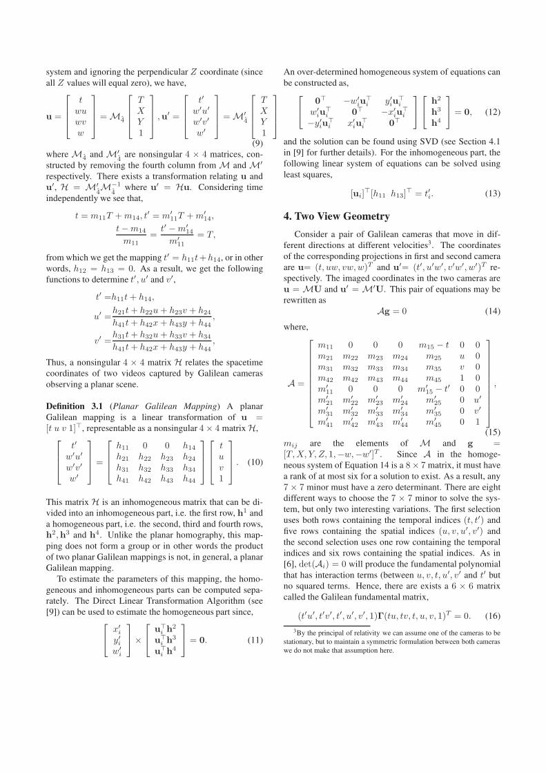
Figure 2. Epipolar Surface. The videopoint in the second video

corresponding to a space-time point in the first video must lie on

this surface.

However, in all the eight variations (of different minors),

nine interaction terms do not exist all, i.e., out of a total of

36 possible interaction terms only 27 appear.

Definition 4.1 (Galilean Fundamental Matrix) If u and u′

are videopoints corresponding to the same worldline under

two Galilean cameras, there exists a 6×6 matrix Γ referred

to as the Galilean Fundamental Matrix such that,

t′u′

t′v′

t′

u′

v′

1

T

0 0 0 f1 f2 f3

0 0 0 f4 f5 f6

0 0 0 f7 f8 f9

f10 f11 f12 f13 f14 f15

f16 f17 f18 f19 f20 f21

f22 f23 f24 f25 f26 f27

tu

tv

t

u

v

1

= 0.

Γ can be written more compactly as,

Γ =

(

0 ∆F′

∆F F00

)

, (17)

where F00 is the fundamental matrix between the image in

the first video at time t = 0 and the image in the second

video at time t′ = 0, and (∆F, ∆F′) are matrices that

capture information about the velocity of each camera as

will be seen presently.

4.1. Epipolar Geometry

Unless there is zero motion, no epipoles (single image

points of the opposite camera center) in the usual sense ex-

ist. In general, epipolar lines (or curves) in the usual sense

do not exist either, instead there are epipolar surfaces in one

camera corresponding to a point in the other camera. These

surfaces are defined by setting a spatiotemporal point in one

camera, i.e. (t′, u′, v′) and applying the Galilean fundamen-

tal matrix. The surface is defined by the

s1tu + s2tv + s3t + s4u + s5v + s6 = 0

where s = [s1, . . . s6] is computed as

s = [t′u′, t′v′, t′, u′, v′, 1]Γ.

An example of this surface is plotted in Figure 2. It can

be seen that this surface is ruled, since the intersection with

each time plane is a line (corresponding to the classic epipo-

lar line of that image).

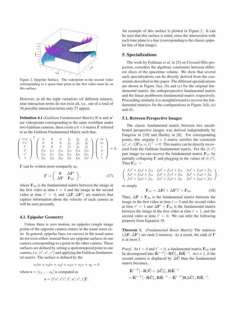
5. Specializations

The work by Feldman et al. in [5] on Crossed-Slits pro-

jection, considers the algebraic constraints between differ-

ent slices of the spacetime volume. We show that several

such specializations can be directly derived from the con-

straints described in this paper. The different specializations

are shown in Figure 3(a), (b) and (c) for the original fun-

damental matrix, the orthoperspective fundamental matrix

and the linear pushbroom fundamental matrix respectively.

Proceeding similarly it is straightforward to recover the fun-

damental matrices for the configurations in Figure 3(d), (e)

and (f).

5.1. Between Perspective Images

The classic fundamental matrix between two uncali-

brated perspective images was derived independently by

Faugeras in [10] and Hartley in [8]. For corresponding

points, this singular 3 × 3 matrix satisfies the constraint

[u′, v′, 1]F[u, v, 1]⊤ = 0. This matrix can be directly recov-

ered from the Galilean fundamental matrix. For the (t, t′)pair image we can recover the fundamental matrix Ftt′ by

partially collapsing Γ and plugging in the values of (t, t′).Thus Ftt′ =(

f1t′ + f10t + f13 f2t

′ + f11t + f14 f3t′ + f12t + f15

f4t′ + f16t + f19 f5t

′ + f17t + f20 f6t′ + f18t + f21

f7t′ + f22t + f25 f8t

′ + f23t + f26 f9t′ + f24t + f27

)

,

or simply

Ftt′ = ∆Ft + ∆F′t′ + F00. (18)

Thus, ∆F + F00 is the fundamental matrix between the

image in the first video at time t = 0 and the second video

at time t′ = 1 and ∆F′ + F00 is the fundamental matrix

between the image in the first video at time t = 1, and the

second video at time t′ = 0. We can infer the following

property from Equation 18.

Theorem 1. (Fundamental Boost Matrix) The matrices

(∆F, ∆F′) are rank-2 matrices. As a result, the rank of Γ

is at most 5.

Proof. At t = 0 and t′ = 0, a fundamental matrix F00 can

be decomposed into K′−T [−RC]×RK−1. At t = 1, if the

second camera is displaced by ∆C then the fundamental

matrix becomes,

K′−T [−R(C + ∆C)]×RK−1

= K′−T [−RC]×RK−1 − K′−T [R∆C]×RK−1.

(a) (b) (c)

(d) (e) (f)Figure 3. Specializations. “Fundamental” matrices can be recovered between (a) a pair of perspective images, (b) an EPI and a perspective

images, (c) a pair of EPIs, (d) a pair of LP images, (e) a LP and an EPI, (f) a LP and a perspective images

From Equation 18,

= F00 + ∆F

= F10.

Since [∆C]× is a skew-symmetric matrix, it follows that

∆F is a rank 2 matrix. The left 6×3 submatrix or the upper

3×6 submatrix of Γ are both therefore rank 2 matrices, and

Γ has a rank of at most 5. �

5.2. Between Linear Pushbroom Images

If the camera motion satisfies the conditions described

in [6], linear pushbroom images can be recovered from a

horizontal slice of the video volume. Between two such

images, the LP fundamental matrix was derived by Gupta

and Hartley in [6]. The relationship captured by this matrix

is expressed as (t′v′, t′, v′, 1)Fuu′(tv, t, v, 1)T = 0. This

4 × 4 matrix too can be directly derived from Γ. Thus,

given (u, u′), we can compute Fuu′ =

0 00 0

f17 f18 + f16u

f11u′ + f23 f22u + f24 + (f10u + f12)u

′

(19)

f5 f4u + f6

f2u′ + f8 f7u + f9 + (f1u + f3)u

′

f20 f19u + f21

f14u′ + f26 f25u + f27 + (f13u + f15)u

′

.

It can be observed that the structure of the matrix is the same

as the one derived in [6].

5.3. Between Epipolar Plane Images

Epipolar plane images were defined by Bolles et al. in

[2] as the collection of epipolar lines that correspond to one

epipolar plane in the world. We can recover the fundamental

matrix between two EPIs. In this case it has a form similar

to the LP fundamental matrix,

0 00 0

f10 f12 + f11v

f16v′ + f22 f23v + f24 + (f17v + f18)v

′

(20)

f1 f2v + f3

f2v′ + f7 f8v + f9 + (f5v + f6)v

′

f13 f14v + f15

f19v′ + f25 f26v + f27 + (f20v + f21)v

′

.

5.4. Between a Pushbroom and a Perspective Image

Recently in [11], Khan et al. derived the 4 × 3perspective-orthoperspective fundamental matrix between

a pushbroom image and a perspective image. The

relationship captured by this matrix is expressed as

(t′v′, t′, v′, 1)Fu′t(u, v, 1)T = 0. This matrix can also be

directly derived from Γ. Thus, given (t, u′), we can com-

pute Ftu′ =

f4 f5

f1u′ + f7 f2u

′ + f8

f16t + f19 f17t + f20

f10tu′ + f22t + f13u

′ + f25 f11tu′ + f23t + f14u

′ + f26

f6

f3u′ + f9

f18t + f21

f12tu′ + f24t + f15u

′ + f27

,

or simply

(

φ∆F′

φt∆F + F00

)

, where φ =

(

0 1 0u′ 0 1

)

.

Similarly, it is straightforward to recover Fvu′ the funda-

mental matrices between an EPI and an LP image, and Ftv′

between an EPI and a perspective image.

6. Normalized Linear Algorithm

A linear algorithm can used to estimate the parameters

of Γ. Equation 17 can be rewritten as the homogeneous

system Aγ = 0 where γ = [f1, · · · , f27]T is a 27-vector,

constructed from the non-zero elements of Γ and A is a

Objective

Given n ≥ 26 matches from corresponding videolines, estimate

the Galilean fundamental matrix Γ such that p′T Γp = 0.

Algorithm

1. Normalization: Normalize the coordinates through an ap-

propriate scaling and translation.

2. Linear Solution: Perform singular value decomposition on

A and determine Γ by selecting the singular vector corre-

sponding to the smallest singular value of A and reconstruct-

ing a 6 × 6 matrix.

3. Rank Constraint: Set the smallest singular value of Γ to

zero, enforce the rank 5 constraint.

4. Denormalization: Denormalize Γ according to the original

scaling and translation.

Figure 4. A linear algorithm for estimating Γ

matrix constructed from spatiotemporal coordinates of cor-

responding points. If noiseless points correspond exactly

to each other the rank of A is 26 and the null-vector of Acorresponds to an estimate of γ. In the presence measure-

ment noise, the 27th singular value will be non zero. In

that case, the singular vector corresponding to the smallest

singular value of A can be used as an estimate of γ. The

rank constraints on Γ can be enforced post facto by setting

the smallest singular values of Γ to zero and reconstructing

the matrix. Of course, as with other linear algorithms of this

sort, to obtain good estimates it is important to appropriately

normalize the data (see Section 4.4 of [9]). Lastly, to obtain

a meaningful solution, A has to have a rank of more than

26. It is emphasized that to ensure the rank of A is greater

than 17, correspondences from different videopoints of the

same worldpoint must be used. For instance, if videolines

of a static world point in the scene of length n are associated

in both cameras, there are n2 rows that should be added to

A.

7. Experimentation

An experiment was conducted where two cameras were

placed on a moving walkway 8 feet apart, looking at differ-

ent angles and moving at approximately 2 miles per hour in

the same direction. A pair of 1000 frame sequences were

recorded at a resolution of 240 × 360 by two SONY HDV

cameras (images were downsampled) and 22 videopoints

were tracked across 6 frames in each of the two videos

(frames 971 to 976 in both sequences). The motion of

the cameras was not perpendicular to the optical axis of

either camera. At 30 fps, the distance traversed by both

cameras during this period was about 98 feet, and the dis-

tance traveled in between successive frames was approxi-

mately 1.2 inches. Three slices of this video are shown in

t- coordinate

v- c

oo

rdin

ate

e

200 400 600 800 1000 1200 1400 1600 1800 2000

100

200

300

400

500

600

700

t -coordinate

u -c

oord

inate

200 400 600 800 1000 1200 1400 1600 1800 2000

50

100

150

200

250

300

350

400

450

v -coordinate

u- c

oo

rdin

ate

100 200 300 400 500 600 700

50

100

150

200

250

300

350

400

450

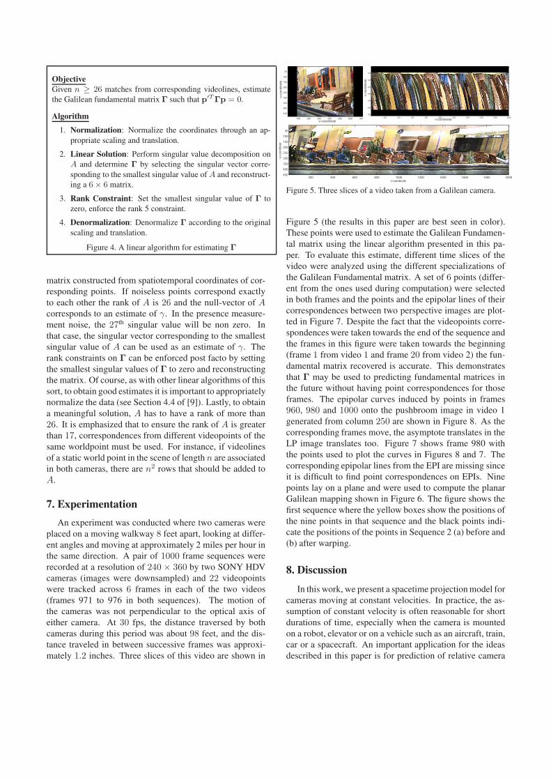
Figure 5. Three slices of a video taken from a Galilean camera.

Figure 5 (the results in this paper are best seen in color).

These points were used to estimate the Galilean Fundamen-

tal matrix using the linear algorithm presented in this pa-

per. To evaluate this estimate, different time slices of the

video were analyzed using the different specializations of

the Galilean Fundamental matrix. A set of 6 points (differ-

ent from the ones used during computation) were selected

in both frames and the points and the epipolar lines of their

correspondences between two perspective images are plot-

ted in Figure 7. Despite the fact that the videopoints corre-

spondences were taken towards the end of the sequence and

the frames in this figure were taken towards the beginning

(frame 1 from video 1 and frame 20 from video 2) the fun-

damental matrix recovered is accurate. This demonstrates

that Γ may be used to predicting fundamental matrices in

the future without having point correspondences for those

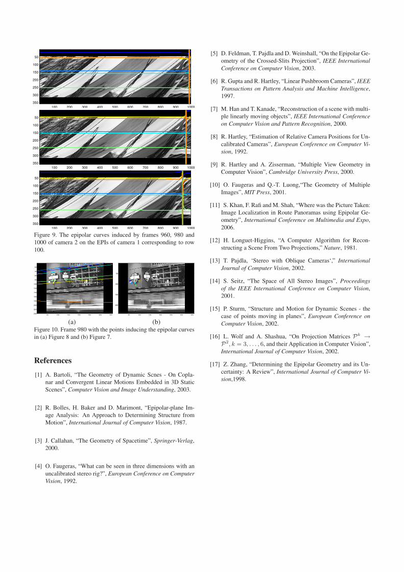
frames. The epipolar curves induced by points in frames

960, 980 and 1000 onto the pushbroom image in video 1

generated from column 250 are shown in Figure 8. As the

corresponding frames move, the asymptote translates in the

LP image translates too. Figure 7 shows frame 980 with

the points used to plot the curves in Figures 8 and 7. The

corresponding epipolar lines from the EPI are missing since

it is difficult to find point correspondences on EPIs. Nine

points lay on a plane and were used to compute the planar

Galilean mapping shown in Figure 6. The figure shows the

first sequence where the yellow boxes show the positions of

the nine points in that sequence and the black points indi-

cate the positions of the points in Sequence 2 (a) before and

(b) after warping.

8. Discussion

In this work, we present a spacetime projection model for

cameras moving at constant velocities. In practice, the as-

sumption of constant velocity is often reasonable for short

durations of time, especially when the camera is mounted

on a robot, elevator or on a vehicle such as an aircraft, train,

car or a spacecraft. An important application for the ideas

described in this paper is for prediction of relative camera

−8 −7 −6 −5 −4 −3

10

20

30

40

50

60

70

u

Sequence 1 (Perspective−Perspective)v

−14 −12 −10 −8 −6 −4 −2 0 2 4

6.3

6.4

6.5

6.6

6.7

6.8

6.9

7

7.1

7.2

u

Sequence 1 (EPI−EPI)

t

20 22 24 26 28 30 32 34 36 38

6.3

6.4

6.5

6.6

6.7

6.8

6.9

7

7.1

7.2

v

Sequence 1 (Pushbroom−Pushbroom)

t

−14 −12 −10 −8 −6 −4 −2 0 2 4

6.3

6.4

6.5

6.6

6.7

6.8

6.9

7

7.1

7.2

u

Sequence 1 (EPI−Pushbroom)

t

−14 −12 −10 −8 −6 −4 −2 0 2 4

6.3

6.4

6.5

6.6

6.7

6.8

6.9

7

7.1

7.2

u

Sequence 1 (EPI−Perspective)

t

20 22 24 26 28 30 32 34 36 38

6.3

6.4

6.5

6.6

6.7

6.8

6.9

7

7.1

7.2

v

Sequence 1 (Pushbroom−Perspective)

t

4 5 6 7 8 9

−80

−60

−40

−20

0

20

40

60

u

Sequence 2 (Perspective−Perspective)

v

−2 0 2 4 6 8 10 12 14 16

1.5

1.55

1.6

1.65

1.7

1.75

1.8

1.85

1.9

1.95

u

Sequence 2 (EPI−EPI)

t

−26 −24 −22 −20 −18 −16 −14 −12 −10 −8

1.7

1.71

1.72

1.73

1.74

1.75

v

Sequence 2 (Pushbroom−Pushbroom)

t

−26 −24 −22 −20 −18 −16 −14 −12 −10 −8

1.7

1.71

1.72

1.73

1.74

1.75

v

Sequence 2 (EPI−Pushbroom)

t

−15 −10 −5 0 5

−600

−500

−400

−300

−200

−100

0

100

200

300

400

u

Sequence 2 (EPI−Perspective)

v

−15 −10 −5 0 5

−600

−500

−400

−300

−200

−100

0

100

200

300

400

u

Sequence 2 (Pushbroom−Perspective)

v

(a) (b) (c) (d) (e) (f)

Figure 11. Corresponding points and their epipolar curves. (a) Between two perspective images (b) Between two LP images (c) Between

two EPIs (d) Between a LP image and an EPI (e) Between a LP image and a perspective (f) Between an EPI and a perspective.

(a) (b)

Figure 6. Videopoints mapped using the planar Galilean mapping.

Yellow squares indicate the position of the points in Sequence 1,

black points indicate the position of (a) corresponding points in

Sequence 2 and (b) corresponding points after warping.

50 100 150 200 250 300 350

20

40

60

80

100

120

140

160

180

200

220

24050 100 150 200 250 300 350

20

40

60

80

100

120

140

160

180

200

220

240

Figure 7. Recovering the fundamental matrix between frame 1 in

sequence 1 and frame 20 in sequence 2 from the Galilean funda-

mental matrix. The Galilean fundamental matrix was computed

from videopoints in six frames (971 to 976 in both sequences).

position. When cameras move, the degree of overlap be-

tween their fields of view usually changes and when the

fields of view become disjoint, estimation of relative cam-

era position becomes impossible. However, if the motion of

the cameras follow some structured motion (like constant

velocity) the ideas presented here can be used to predict the

fundamental matrix relating views even when their fields of

view are disjoint. We investigate the relative geometry re-

lating a pair of such cameras in planar and general scenes.

We show how three known fundamental matrices are spe-

cializations of this matrix and could be readily recovered

from the proposed fundamental matrix, providing a unify-

100 200 300 400 500 600 700 800 900 1000

50

100

150

200

100 200 300 400 500 600 700 800 900 1000

50

100

150

200

100 200 300 400 500 600 700 800 900 1000

50

100

150

200

Figure 8. The epipolar curves induced by frames 960, 980 and

1000 of camera 2 on the pushbroom images of camera 1 corre-

sponding to column 250.

ing link between the classic fundamental matrix and the LP

fundamental matrix. In addition we describe three new fun-

damental matrices that can also be recovered. In the future,

we intend to investigate the application of different motion

models, such as a constant acceleration model, and study

the relationships between three or more Galilean cameras.

Acknowledgements

The authors thank Takeo Kanade for his useful com-

ments and suggestions. This work was funded by the

Disruptive Technologies Office, Video Analysis and Con-

tent Extraction (VACE) Program - Phase III, Contract No.

NBCHC060105 issued by the Department of the Interior.

The view and conclusions are those of the authors, not of

the US Government or its agencies.

100 200 300 400 500 600 700 800 900 1000

50

100

150

200

250

300

350

100 200 300 400 500 600 700 800 900 1000

50

100

150

200

250

300

350

100 200 300 400 500 600 700 800 900 1000

50

100

150

200

250

300

350

Figure 9. The epipolar curves induced by frames 960, 980 and

1000 of camera 2 on the EPIs of camera 1 corresponding to row

100.

50 100 150 200 250 300 350

20

40

60

80

100

120

140

160

180

200

220

24050 100 150 200 250 300 350

50

100

150

200

(a) (b)Figure 10. Frame 980 with the points inducing the epipolar curves

in (a) Figure 8 and (b) Figure 7.

References

[1] A. Bartoli, “The Geometry of Dynamic Scnes - On Copla-

nar and Convergent Linear Motions Embedded in 3D Static

Scenes”, Computer Vision and Image Understanding, 2003.

[2] R. Bolles, H. Baker and D. Marimont, “Epipolar-plane Im-

age Analysis: An Approach to Determining Structure from

Motion”, International Journal of Computer Vision, 1987.

[3] J. Callahan, “The Geometry of Spacetime”, Springer-Verlag,

2000.

[4] O. Faugeras, “What can be seen in three dimensions with an

uncalibrated stereo rig?”, European Conference on Computer

Vision, 1992.

[5] D. Feldman, T. Pajdla and D. Weinshall, “On the Epipolar Ge-

ometry of the Crossed-Slits Projection”, IEEE International

Conference on Computer Vision, 2003.

[6] R. Gupta and R. Hartley, “Linear Pushbroom Cameras”, IEEE

Transactions on Pattern Analysis and Machine Intelligence,

1997.

[7] M. Han and T. Kanade, “Reconstruction of a scene with multi-

ple linearly moving objects”, IEEE International Conference

on Computer Vision and Pattern Recognition, 2000.

[8] R. Hartley, “Estimation of Relative Camera Positions for Un-

calibrated Cameras”, European Conference on Computer Vi-

sion, 1992.

[9] R. Hartley and A. Zisserman, “Multiple View Geometry in

Computer Vision”, Cambridge University Press, 2000.

[10] O. Faugeras and Q.-T. Luong,“The Geometry of Multiple

Images”, MIT Press, 2001.

[11] S. Khan, F. Rafi and M. Shah, “Where was the Picture Taken:

Image Localization in Route Panoramas using Epipolar Ge-

ometry”, International Conference on Multimedia and Expo,

2006.

[12] H. Longuet-Higgins, “A Computer Algorithm for Recon-

structing a Scene From Two Projections,” Nature, 1981.

[13] T. Pajdla, ‘Stereo with Oblique Cameras‘,” International

Journal of Computer Vision, 2002.

[14] S. Seitz, “The Space of All Stereo Images”, Proceedings

of the IEEE International Conference on Computer Vision,

2001.

[15] P. Sturm, “Structure and Motion for Dynamic Scenes - the

case of points moving in planes”, European Conference on

Computer Vision, 2002.

[16] L. Wolf and A. Shashua, “On Projection Matrices Pk →

P2, k = 3, . . . , 6, and their Application in Computer Vision”,

International Journal of Computer Vision, 2002.

[17] Z. Zhang, “Determining the Epipolar Geometry and its Un-

certainty: A Review”, International Journal of Computer Vi-

sion,1998.